Unique entanglement dynamics of two-qubit separable and Werner states in a discrete qubit environment

Abstract

This study investigates how the entanglement dynamics of separable and Werner states differ in a finite Markovian N-qubit environment under two environmental conditions: homogeneous and white noise. We demonstrate that in a homogeneous environment, the entanglement dynamics of the separable state is influenced by interactions between subsystems $\omega_{\mathcal{S}_{1}\mathcal{S}_{2}}$ and the environment $\Gamma$, while for Werner states it depends solely on $\Gamma$. Both states exhibit unique properties that enable us to distinguish the initial state through their entanglement dynamics and maximum concurrence. In contrast, in a white noise environment, the decay time of entanglement is determined only by the size of the environment and the randomness of interaction strengths, underscoring the significant role of environmental factors in quantum dynamics.

I Introduction

Entanglement is a quantum phenomenon that arises when two particles interact. The interaction transforms the two-particle wavefunction into one inseparable wavefunction that can no longer be described by its local constituents [1]. This strange property of entanglement, combined with the probabilistic nature of quantum systems, enables the solution of complex mathematical problems through exponentially rapid computations [2]. Entanglement applications include quantum cryptography [3, 4, 5], quantum dense coding [6, 7, 8, 9, 10], quantum teleportation [11, 12, 13], and quantum algorithms [14, 15, 16].

However, entanglement fragility due to environmental noise prevents its realization for practical purposes [17]. For instance, coupling a pure bipartite system to a thermal reservoir invariably leads to entanglement decay [18]. In contrast, some initially entangled states subjected to vacuum noise exhibit asymptotic entanglement decay [19, 18]. On the other hand, Sese and Galapon [20] examined a qubit in a discrete Markovian homogeneous environment and found that the coherence of a system periodically recovers its dissipated information, resulting in an exact recurrence.

In response, we investigate the entanglement dynamics of a two-qubit system initially prepared in two ways, namely, separable and Werner states. These states will be examined with two types of Markovian environments: homogeneous and white noise. The Markovian condition sets the calculation to be independent of the previous calculations. The homogeneous environment assumes that all qubit environments interact with the same coupling strength. However, in a white noise environment, each qubit’s interaction strength is chosen at random from a uniform distribution. We then derive the reduced density matrix $\rho_{\mathcal{S}}(t)$ and compute the concurrence to determine the entanglement dynamics of the states. The results show that the entanglement dynamics of the states considered are highly contingent on the initial preparation, whereas the entanglement decay only happens due to the randomness of the environmental interactions. This work aims to identify the specific cause of entanglement decay in our model, which is relevant in entanglement manipulation and preservation.

The paper is arranged as follows. In Sec. II, we provide the model of interaction and derivation of $\rho_{\mathcal{S}}(t)$. We then calculate the concurrence of two different states in Sec. III in a homogeneous (Sec. III.1) and white noise environment (Sec. III.2). Lastly, we provide a conclusion in Sec. IV.

II Model

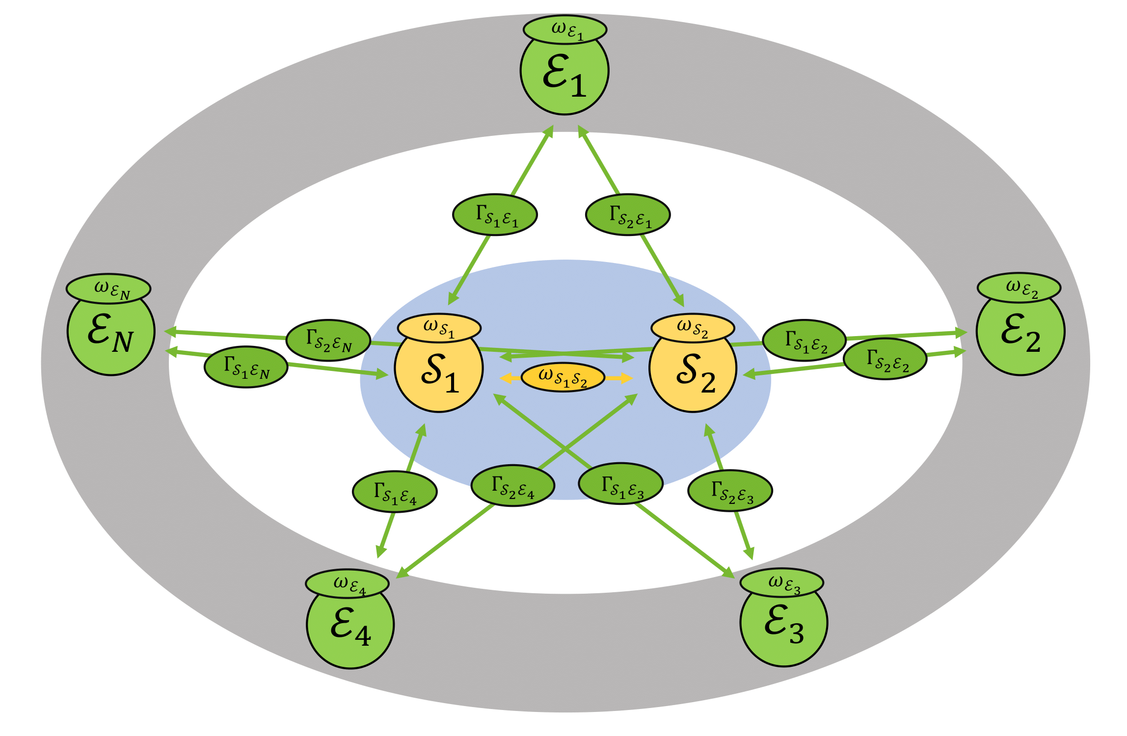
Figure 1: A similar sketch of composite system and its Hamiltonian from Ref. [21].

Our system of interest is a bipartite qubit system $\mathcal{S}$ consists of two subsystems, $\mathcal{S}_{1}$ and $\mathcal{S}_{2}$. Each subsystem of $\mathcal{S}$ interacts directly with an $N$-qubit environment $\mathcal{E}$, where every qubit of $\mathcal{E}$ is initially non-interacting with one another. In particular, $\mathcal{E}$ refers to the qubits outside of our system of interest. The total Hamiltonian consists of $\mathcal{S}$’s self-Hamiltonian $\hat{H}_{\mathcal{S}}$, $\mathcal{E}$’s self-Hamiltonian $\hat{H}_{\mathcal{E}}$, and the interaction Hamiltonian $\hat{H}_{\text{int}}$,

$$\hat{H}_{\mathcal{S}} = \frac{\hbar}{2}\omega_{\mathcal{S}_{1}}\hat{\sigma}^{z}_{\mathcal{S}_{1}}+\frac{\hbar}{2}\omega_{\mathcal{S}_{2}}\hat{\sigma}^{z}_{\mathcal{S}_{2}},$$

$$\hat{H}_{\mathcal{E}} = \frac{\hbar}{2}\sum_{k=1}^{N}\omega_{\mathcal{E}_{k}}\hat{\sigma}^{z}_{\mathcal{E}_{k}},$$ (1)

$$\hat{H}_{\text{int}} = \frac{\hbar}{2}\omega_{\mathcal{S}_{1}\mathcal{S}_{2}}\hat{\sigma}^{z}_{\mathcal{S}_{1}}\hat{\sigma}^{z}_{\mathcal{S}_{2}}+\frac{\hbar}{2}\sum_{k=1}^{N}\Gamma_{\mathcal{S}_{1}\mathcal{E}_{k}}\hat{\sigma}^{z}_{\mathcal{S}_{1}}\hat{\sigma}^{z}_{\mathcal{E}_{k}}$$

$$+ \frac{\hbar}{2}\sum_{k=1}^{N}\Gamma_{\mathcal{S}_{2}\mathcal{E}_{k}}\hat{\sigma}^{z}_{\mathcal{S}_{2}}\hat{\sigma}^{z}_{\mathcal{E}_{k}}.$$

The coupling strengths $\omega_{\mathcal{S}_{1}}$, $\omega_{\mathcal{S}_{2}}$, $\omega_{\mathcal{E}_{k}}$, $\omega_{\mathcal{S}_{1}\mathcal{S}_{2}}$, $\Gamma_{\mathcal{S}_{1}\mathcal{E}_{k}}$, and $\Gamma_{\mathcal{S}_{2}\mathcal{E}_{k}}$ are $\in\mathbb{R}$, while $k=1,2,3,\dots,N$ describe the individual qubit in $\mathcal{E}$ as shown in Figure 1. Also, $\omega_{\mathcal{S}_{1}\mathcal{S}_{2}}$ represents the interaction between $\mathcal{S}_{1}$ and $\mathcal{S}_{2}$, whereas $\Gamma_{\mathcal{S}_{1}\mathcal{E}_{k}}$ and $\Gamma_{\mathcal{S}_{2}\mathcal{E}_{k}}$ are the interactions between the $k$th qubit environment and $\mathcal{S}_{1}$ and $\mathcal{S}_{2}$, respectively. The Hamiltonian was also used by Ref. [21]. Note that Eq. (II) is a time-independent ising interaction confined in the $z$-basis, allowing us to calculate the time evolution operator with ease. Hence, the resulting reduced density matrix $\rho_{\mathcal{S}}(t)$

$$\rho_{\mathcal{S}}(t)=\sum_{l,m,n,o=0}^{1}a_{lm}a^{*}_{no}r_{lmno}(t)\ket{lm}\bra{no},$$ (2)

with $r_{lmno}(t)$ expressed as,

$$r_{0000}(t) = r_{0101}(t)=r_{1010}(t)=r_{1111}(t)=1,$$

$$r_{\begin{subarray}{c}0010\\ 0111\end{subarray}}(t) = r_{\begin{subarray}{c}1000\\ 1101\end{subarray}}^{*}(t)=\text{exp}[-it(\omega_{\mathcal{S}_{1}}\pm\omega_{\mathcal{S}_{1}\mathcal{S}_{2}})]\prod_{k=1}^{N}\big{(}|\alpha_{k}|^{2}\text{exp}[-it\Gamma_{\mathcal{S}_{1}\mathcal{E}_{k}}]+|\beta_{k}|^{2}\text{exp}[it\Gamma_{\mathcal{S}_{1}\mathcal{E}_{k}}]\big{)},$$

$$r_{\begin{subarray}{c}0001\\ 1011\end{subarray}}(t) = r_{\begin{subarray}{c}0100\\ 1110\end{subarray}}^{*}(t)=\text{exp}[-it(\omega_{\mathcal{S}_{2}}\pm\omega_{\mathcal{S}_{1}\mathcal{S}_{2}})]\prod_{k=1}^{N}\big{(}|\alpha_{k}|^{2}\text{exp}[-it\Gamma_{\mathcal{S}_{2}\mathcal{E}_{k}}]+|\beta_{k}|^{2}\text{exp}[it\Gamma_{\mathcal{S}_{2}\mathcal{E}_{k}}]\big{)},$$ (3)

$$r_{\begin{subarray}{c}0011\\ 0110\end{subarray}}(t) = r_{\begin{subarray}{c}1100\\ 1001\end{subarray}}^{*}(t)=\text{exp}[-it(\omega_{\mathcal{S}_{1}}\pm\omega_{\mathcal{S}_{2}})]\prod_{k=1}^{N}\big{(}|\alpha_{k}|^{2}\text{exp}[-it(\Gamma_{\mathcal{S}_{1}\mathcal{E}_{k}}\pm\Gamma_{\mathcal{S}_{2}\mathcal{E}_{k}})]+|\beta_{k}|^{2}\text{exp}[it(\Gamma_{\mathcal{S}_{1}\mathcal{E}_{k}}\pm\Gamma_{\mathcal{S}_{2}\mathcal{E}_{k}})]\big{)},$$

where the subscripts represent the arrangement of plus or minus based on their respective equations. We denote the nontrivial terms in Eq. (II) as decoherence factors that describe the system’s interference over time $t$. These decoherence factors appear to be in similar form from several studies [22, 23, 20, 21] but with some additional factors due to the inclusion of several terms in the Hamiltonian. We will later found that only the interaction strengths $\omega_{\mathcal{S}_{1}\mathcal{S}_{2}}$, $\Gamma_{\mathcal{S}_{1}\mathcal{E}_{k}}$, $\Gamma_{\mathcal{S}_{2}\mathcal{E}_{k}}$, and $N$ will affect the entanglement dynamics. Furthermore, since Eq. (II) is independent of the system preparation, we can express the time evolution of any initial state in terms of Eq. (2).

In the following section, we will utilize Eq. (2) as a representation of any initially prepared state to obtain the entanglement dynamics through concurrence.

III Concurrence

Concurrence is a standard quantitative measurement of entanglement for two qubits. The generalized concurrence formula is given by Wootters [24]

$$C(\rho)=\text{max}\{0,\nu_{1}-\nu_{2}-\nu_{3}-\nu_{4}\},$$ (4)

where $\nu$s denote the square roots of the eigenvalues of $\rho\tilde{\rho}$ in decreasing order, with $\nu_{1}$ being the highest. To calculate $\tilde{\rho}$, apply the spin-flip operation ( $\tilde{}$ ) to the reduced density matrix $\rho$, which is defined as

$$\tilde{\rho}=(\sigma^{y}\otimes\sigma^{y})\rho^{*}(\sigma^{y}\otimes\sigma^{y}).$$ (5)

To support our findings, we briefly demonstrate the purity-based separability criterion proposed by Flores and Galapon [25] in Appendix A.

III.1 Homogeneous environment

In a homogeneous environment, we set every qubit environment to be the same. That is, $|\alpha_{k}|^{2}=|\beta_{k}|^{2}=|\alpha|^{2}=|\beta|^{2}=1/2$ and their interaction strengths as $\Gamma_{\mathcal{S}_{1}\mathcal{E}_{k}}=\Gamma_{\mathcal{S}_{2}\mathcal{E}_{k}}=\Gamma$. This simplifies our decoherence factor into this form

$$r_{\begin{subarray}{c}0010\\ 0111\end{subarray}} = r_{\begin{subarray}{c}1000\\ 1101\end{subarray}}^{*}=e^{-it(\omega_{\mathcal{S}_{1}}\pm\omega_{\mathcal{S}_{1}\mathcal{S}_{2}})}\sum_{k=0}^{N}\begin{pmatrix}N\\ k\end{pmatrix}|\alpha|^{2k}|\beta|^{2(N-k)}\text{exp}[i\Gamma(N-2k)t],$$

$$r_{\begin{subarray}{c}0001\\ 1011\end{subarray}} = r_{\begin{subarray}{c}0100\\ 1110\end{subarray}}^{*}=e^{-it(\omega_{\mathcal{S}_{2}}\pm\omega_{\mathcal{S}_{1}\mathcal{S}_{2}})}\sum_{k=0}^{N}\begin{pmatrix}N\\ k\end{pmatrix}|\alpha|^{2k}|\beta|^{2(N-k)}\text{exp}[i\Gamma(N-2k)t],$$ (6)

$$r_{0011} = r_{1100}^{*}=e^{-it(\omega_{\mathcal{S}_{1}}+\omega_{\mathcal{S}_{2}})}\sum_{k=0}^{N}\begin{pmatrix}N\\ k\end{pmatrix}|\alpha|^{2k}|\beta|^{2(N-k)}\text{exp}[2i\Gamma(N-2k)t],$$

$$r_{0110} = r_{1001}^{*}=e^{-it(\omega_{\mathcal{S}_{1}}-\omega_{\mathcal{S}_{2}})},$$

which belongs to a class of almost periodic functions [26, 27]. This suggests that the entanglement dynamics manifests as an almost periodic behavior in a homogeneous environment [21].

The following figures show a scaled contour map of concurrence with respect to $\Gamma$, $\omega_{\mathcal{S}_{1}\mathcal{S}_{2}}$, and $t$ for different $N$. The vertical axis is defined as a function of the numerator, which is scaled by the denominator and the horizontal axis.

III.1.1 Separable state

In a bipartite system, a separable state is equivalent to being unentangled if it can be expressed as a convex combination of tensor products from sub-Hilbert space orthonormal bases, that is

$$\ket{\Psi(0)}_{SEP}=(a_{0}\ket{0}_{1}+a_{1}\ket{1}_{1})\otimes(a_{0}\ket{0}_{2}+a_{1}\ket{1}_{2}),$$ (7)

or equivalently,

$$\ket{\Psi(0)}_{SEP}=a_{00}\ket{00}+a_{01}\ket{01}+a_{10}\ket{10}+a_{11}\ket{11}.$$ (8)

We also set the system’s probability densities as $1/2$. In Figure 2, increasing $N$ results in a sharper contour reading, as also shown in Ref. [22]. Moreover, the dynamics of a separable state contains gaps with non-zero asymptotes in the $x$- and $y$-axes. The figure also shows that when the $y$-axis is rational, the concurrence is periodic. In contrast, when it is irrational, the concurrence exhibits no periodicity. Figure 3 supports our earlier claim that entanglement is independent of $\omega_{\mathcal{S}_{1}}$ and $\omega_{\mathcal{S}_{2}}$. It shows that $\omega_{\mathcal{S}_{1}}$ and $\omega_{\mathcal{S}_{2}}$ do not affect the entanglement dynamics of any initially prepared states.

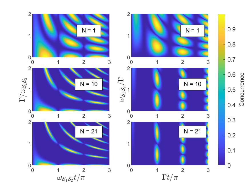
Figure 2: Concurrence contour map of a separable state for $\Gamma$ and $\omega_{\mathcal{S}_{1}\mathcal{S}_{2}}$.

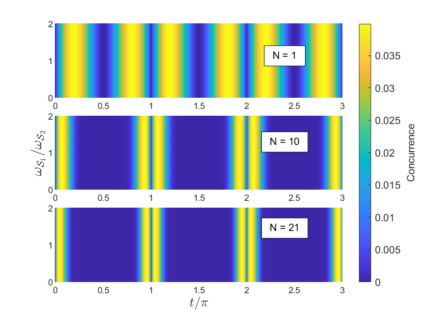
Figure 3: A contour map of $\omega_{\mathcal{S}_{1}}$ and $\omega_{\mathcal{S}_{2}}$ when $\Gamma/\omega_{\mathcal{S}_{1}\mathcal{S}_{2}}=1$.

III.1.2 Werner state

The Werner states is an experimentally occurring quantum state that can be reduced to a mixed or a Bell state depending on the initial purity $\lambda$ given within the $[0,1]$ domain [28]. In general, entanglement becomes limited as the purity decreases [29]. The positive partial transpose (PPT) criterion indicates that the Werner state projected into a Bell basis is separable at $\lambda<1/3$ and entangled at $1/3<\lambda\leq 1$. The Werner states can be expressed as

$$W^{0110}(0) = \lambda\ket{e_{0110}}\bra{e_{0110}}+\frac{1-\lambda}{4}I_{4},$$

$$W^{0011}(0) = \lambda\ket{e_{0011}}\bra{e_{0011}}+\frac{1-\lambda}{4}I_{4},$$ (9)

where

$$\ket{e^{\pm}_{0011}} = \frac{1}{\sqrt{2}}(\ket{00}\pm\ket{11}),$$

$$\ket{e^{\pm}_{0110}} = \frac{1}{\sqrt{2}}(\ket{01}\pm\ket{10}),$$ (10)

are Bell states, and $I_{4}$ as a four-dimensional identity matrix. In a matrix representation, the matrix elements of $W^{0110}(0)$ are

$$W^{0110}_{11}(0) = W^{0110}_{44}=\frac{1-\lambda}{4},$$

$$W^{0110}_{22}(0) = W^{0110}_{33}(0)=\frac{1-\lambda}{4}+\frac{\lambda}{2},$$ (11)

$$W^{0110}_{14}(0) = 0,\quad W^{0110}_{23}(0)=\frac{\lambda}{2},$$

where the rest of the elements are zero. On the other hand, $W^{0011}(0)$ has matrix elements

$$W^{0011}_{11}(0) = W^{0011}_{44}(0)=\frac{1-\lambda}{4}+\frac{\lambda}{2},$$

$$W^{0011}_{22}(0) = W^{0011}_{33}(0)=\frac{1-\lambda}{4},$$ (12)

$$W^{0011}_{14}(0) = \frac{\lambda}{2},\quad W^{0011}_{23}(0)=0,$$

and the rest are zero. Consequently, the general form of a Werner states has a structure of “X” density matrix

$$W(0)=\begin{pmatrix}W_{11}(0)&0&0&W_{14}(0)\\ 0&W_{22}(0)&W_{23}(0)&0\\ 0&W_{23}(0)&W_{33}(0)&0\\ W_{14}(0)&0&0&W_{44}(0)\end{pmatrix}.$$ (13)

Applying the matrix elements in Eqs. (III.1.2) and (III.1.2) to Eq. (2), we can calculate the concurrence of a Werner state. Figure 4 illustrates the dependence of entanglement dynamics on $\lambda$. For instance, when $\lambda=0$, the Werner states become maximally mixed states [28]. But when $\lambda=1$, the Werner states are reduced into Bell states, which are maximally entangled states.

Figures 5 and 6 demonstrate that the entanglement of $W^{0110}$ and $W^{0011}$ are invariant with respect to change in $\omega_{\mathcal{S}_{1}\mathcal{S}_{2}}$, respectively. For instance, the Bell state is already a maximally entangled state, thus, creating additional entanglement from $\omega_{\mathcal{S}_{1}\mathcal{S}_{2}}$ is trivial. Furthermore, we also found that $W^{0110}$ is immune to the homogeneous environment — a manifestation of decoherence-free subspace [30]. In contrast, $W^{0011}$ is only vulnerable to the environment, supporting the Hamiltonian model used by Ref. [23]. For intermediate values of $\lambda$, the maximum concurrence is reduced. Hence, the system fails to achieve maximum entanglement.

The relationship of $\Gamma$ to the Werner states’ dynamics appears to be similar to the separable state but without any gaps. Remarkably, $\ket{e^{\pm}_{0011}}$ and $\ket{e^{\pm}_{0110}}$ can maintain and periodically achieve maximum entanglement, respectively, which is not observed in a separable state. This implies that a separable state will never become a Werner state under the Hamiltonian we considered or vice versa.

While both separable and Werner states can have the same concurrence within the $[0,1)$ range, they still exhibit distinct dynamics. This suggests that both states possess unique properties that allow us to differentiate them based on their dynamics and behavior from the interaction strengths. In Figure 7, the concurrence resembles an isothermal process. Specifically, the relationship between $\Gamma$ and $t$ is inversely proportional for the same concurrence value, which is referred to as isoconcurrence.

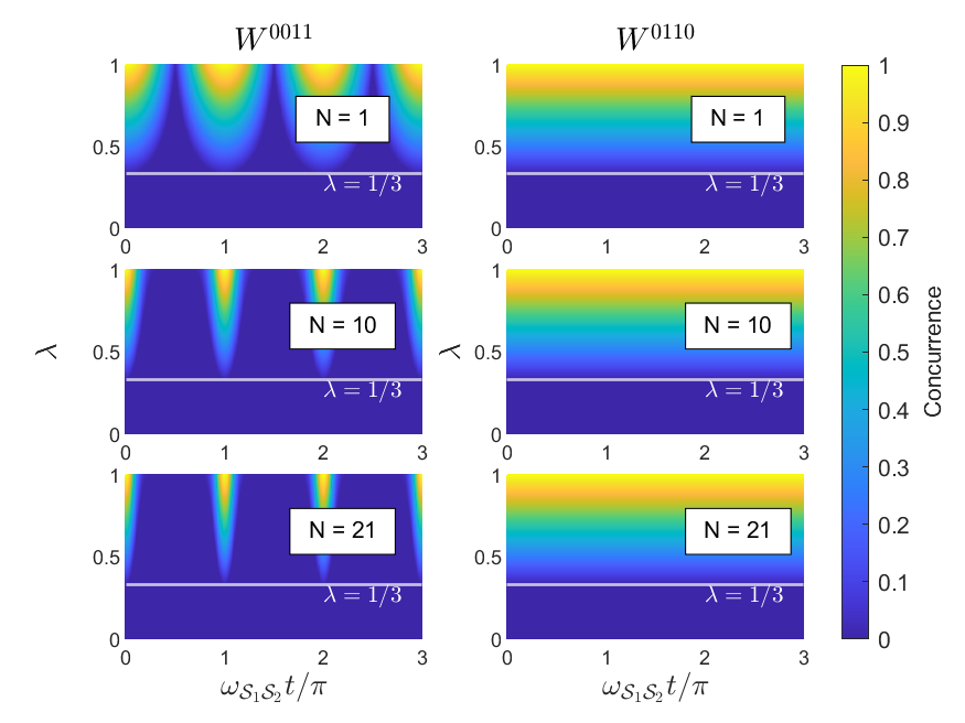
Figure 4: Concurrence of an initially prepared as Werner states in homogeneous environment when $\Gamma/\omega_{\mathcal{S}_{1}\mathcal{S}_{2}}=0.5$.

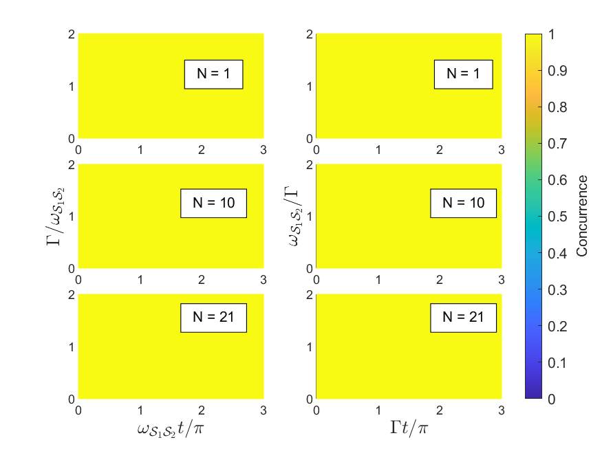
Figure 5: Entanglement dynamics of $W^{0110}$ in a homogeneous environment at $\lambda=1$.

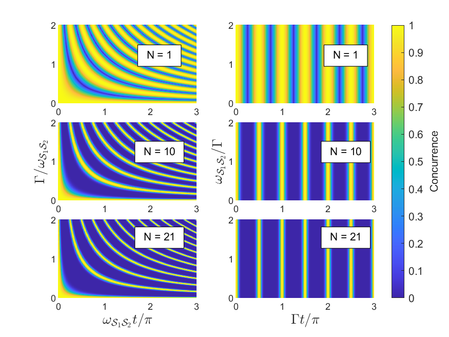
Figure 6: Entanglement dynamics of $W^{0011}$ at $\lambda=1$.

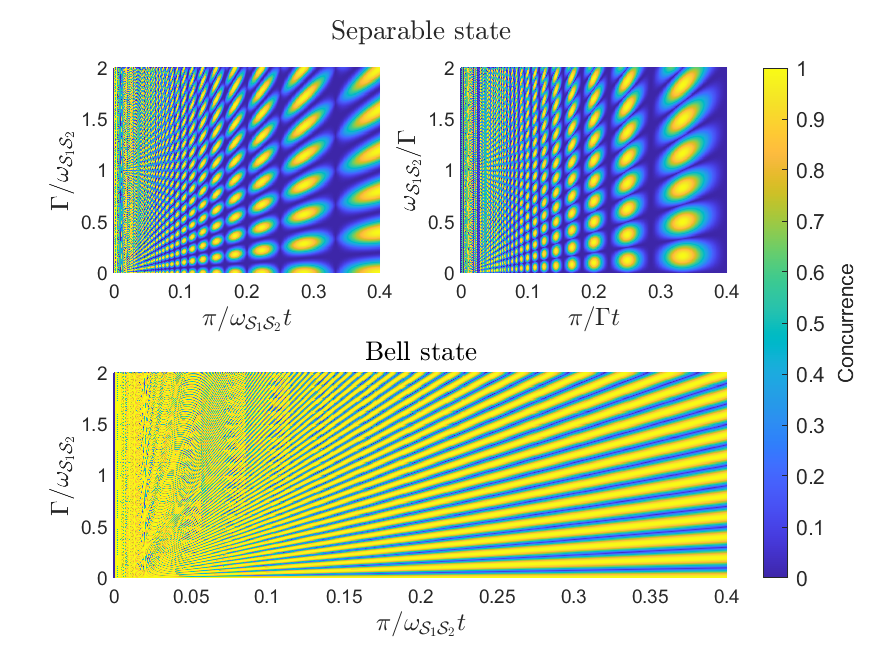
Figure 7: Linearization of concurrence by setting the $x$-axis to $1/x$ with $N=1$.

III.2 White noise

In a chaotic environment like white noise, we use a random number generator (RNG) in MATLAB to randomize $\Gamma_{\mathcal{S}_{1}\mathcal{E}_{k}}$ and $\Gamma_{\mathcal{S}_{2}\mathcal{E}_{k}}$. We then set $\Gamma_{\mathcal{S}_{i}\mathcal{E}_{k}}/\omega_{\mathcal{S}_{1}\mathcal{S}_{2}}$ as the mean $\mu$ of the distribution with a range $f$ away from $\mu$. In the case where $f<\mu$, we utilize the $|\mu-f|$ to prevent any negative interaction strengths in calculations. Since $N$ does not approach the thermodynamic limit, RNG can only generate a sparse set of random numbers within the distribution. Hence, all RNG distributions will just yield similar results.

Nevertheless, Figures 8 to 11 show entanglement decay, which is common in large and chaotic environments. This is because the cardinality of $\mathbb{Q}^{\prime}$ in a continuous range is significantly higher than $\mathbb{Q}$. This results in a large number of different interaction strengths that induce destructive interference and, thus, entanglement dissipation. Although the decay only occurs by randomizing environmental strengths, the dissipation time is invariant to $\mu$ but exponentially scales with the environment size $N$, as shown in Figure 11.

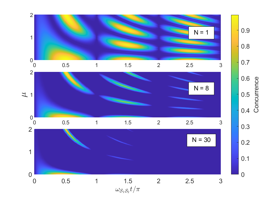
Figure 8: Concurrence of initially separable state with white noise ranging from $[\mu-f,\mu+f]$, where $f=0.1$.

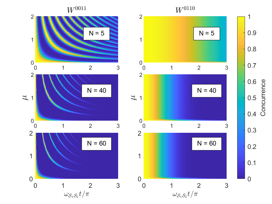
Figure 9: Concurrence of Werner states at $\lambda=1$ with the same white noise setting as Figure 8.

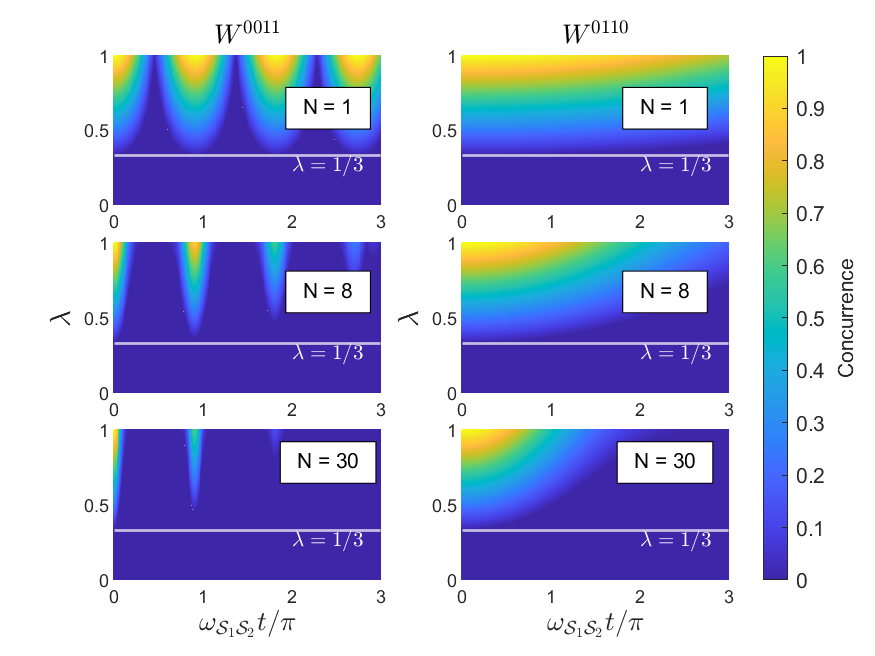
Figure 10: Concurrence of Werner states in a white noise with $\mu=0.5$ and $f=0.1$.

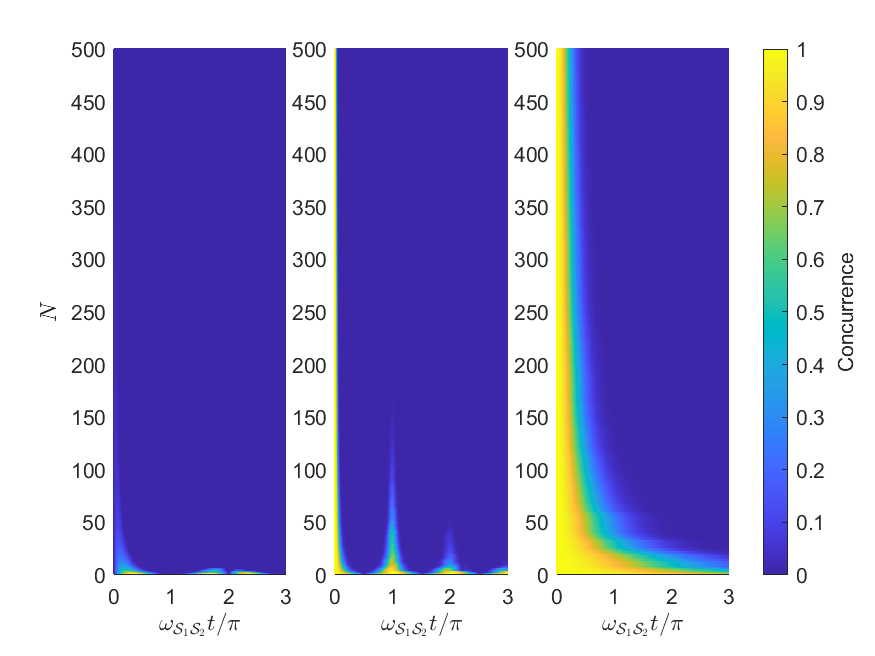
Figure 11: Mapping $N$ in separable (left), $W^{0011}$ (middle), and $W^{0110}$ (right) states at $\lambda=1$ with $\mu=0.5$ and $f=0.1$.

IV Conclusion

We studied the concurrence dynamics of two initially prepared states, namely separable and Werner states, in two environments, such as a homogeneous and white noise environment. In a homogeneous environment, the entanglement dynamics with respect to the interaction strengths are strongly dependent on the prepared state. Specifically, the dynamics of the separable state depends on $\Gamma$ and $\omega_{\mathcal{S}_{1}\mathcal{S}_{2}}$, whereas only $\Gamma$ for Werner states. Furthermore, the separable state contains gaps and never reaches a maximally entangled state, while $\ket{e^{\pm}_{0011}}$ and $\ket{e^{\pm}_{0110}}$ maintain and periodically achieve maximum entanglement, respectively. Hence, the separable and Werner states possess unique properties so that their dynamics is entirely different from each other. On the other hand, placing the states in a white noise environment results in entanglement dissipation, where the time of dissipation exponentially decreases as $N$ increases. We also discovered that the dissipation time is unrelated to the value of the interaction strengths but rather to the randomness of the environment. Our findings allow us to identify a state based on its dynamics in a homogeneous or white noise environment, even without knowledge of the system’s initial preparation.

This work provides a simplified model of how the qubit environment influences the system’s entanglement. One possible extension is to consider a mutually interacting environment, an arbitrary bipartite system, a multipartite system, a comparison of coherence and entanglement, and a simple application to quantum circuits. And lastly, it would be interesting to have an in-depth discussion of the analytical form of entanglement dynamics to validate our results.

Appendix A Purity-based separability criterion

Flores and Galapon [25] proposed a purity-based separability criterion that distinguishes the system between separable and entangled states. This scalar-type criterion has the advantage of allowing us to quantitatively measure the state’s purity. However, the criterion was only consistent with concurrence for a bipartite system, which fortunately applies to our case. The criterion contains the following theorems:

Theorem 1

if $\rho$ is separable, then $\text{Tr}[(\rho)^{2}]\leq\text{Tr}[(\rho^{i})^{2}]$ for all subsystems i.

However, having $\text{Tr}[\rho^{2}]\leq\text{Tr}[(\rho^{i})^{2}]$ for all $i$ will not guarantee $\rho$ to be separable.

Theorem 2

If there exists a subsystem $i$ such that $\text{Tr}[(\rho^{i})^{2}]<\text{Tr}[\rho^{2}]$, then $\rho$ is entangled.

Figure 12 shows that entanglement occurs when the purity is $\text{Tr}[(\rho^{A})^{2}]<\text{Tr}[\rho^{2}]$, where $A$ is an arbitrary subsystem of $\rho$. That is, entanglement occurs when subsystems have less information than the entire system. In contrast, entanglement does not occur when $\text{Tr}[(\rho)^{2}]=\text{Tr}[(\rho^{A})^{2}]$. However, we see a small entanglement measurement when $\text{Tr}[(\rho)^{2}]<\text{Tr}[(\rho^{A})^{2}]$, which exercises the statement mentioned in Theorem 1. Note that this criterion is not an entanglement measurement but rather a tool for distinguishing entangled states from separable states. Furthermore, we observed that purity depends on interaction strengths $\omega_{\mathcal{S}_{1}\mathcal{S}_{2}}$ and $\Gamma$, which is expected because purity is a tool to verify concurrence.

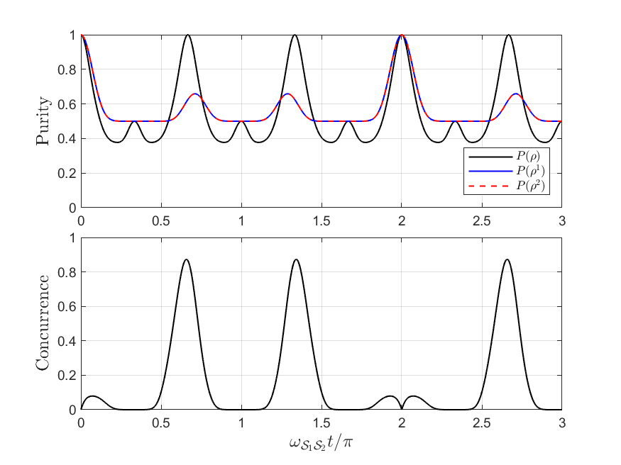
Figure 12: 2D slice of comparison between purity (top) and concurrence (bottom) from parameter $\Gamma/\omega_{\mathcal{S}_{1}\mathcal{S}_{2}}=1.5$.

References

- Schrödinger [1935] E. Schrödinger, Math. Proc. Cambridge Philos. Soc. 31, 555–563 (1935).
- Marella and Parisa [2020] S. T. Marella and H. S. K. Parisa, in Quantum Computing and Communications, edited by Y. Zhao (IntechOpen, Rijeka, 2020) Chap. 5.
- Ekert [1991] A. K. Ekert, Phys. Rev. Lett. 67, 661 (1991).
- Naik et al. [2000] D. S. Naik, C. G. Peterson, A. G. White, A. J. Berglund, and P. G. Kwiat, Phys. Rev. Lett. 84, 4733 (2000).
- Tittel et al. [2000] W. Tittel, J. Brendel, H. Zbinden, and N. Gisin, Phys. Rev. Lett. 84, 4737 (2000).
- Holevo [1973] A. S. Holevo, Probl. Peredachi Inf. (1973).
- Mattle et al. [1996] K. Mattle, H. Weinfurter, P. G. Kwiat, and A. Zeilinger, Phys. Rev. Lett. 76, 4656 (1996).
- Fang et al. [2000] X. Fang, X. Zhu, M. Feng, X. Mao, and F. Du, Phys. Rev. A 61, 022307 (2000).
- Mizuno et al. [2005] J. Mizuno, K. Wakui, A. Furusawa, and M. Sasaki, Phys. Rev. A 71, 012304 (2005).
- Jing et al. [2003] J. Jing, J. Zhang, Y. Yan, F. Zhao, C. Xie, and K. Peng, Phys. Rev. Lett. 90, 167903 (2003).
- Bennett et al. [1993] C. H. Bennett, G. Brassard, C. Crépeau, R. Jozsa, A. Peres, and W. K. Wootters, Phys. Rev. Lett. 70, 1895 (1993).
- Bouwmeester et al. [1997] D. Bouwmeester, J.-W. Pan, K. Mattle, M. Eibl, H. Weinfurter, and A. Zeilinger, Nature 390, 575–579 (1997).
- Sherson et al. [2006] J. F. Sherson, H. Krauter, R. K. Olsson, B. Julsgaard, K. Hammerer, I. Cirac, and E. S. Polzik, Nature 443, 557–560 (2006).
- Jozsa [1997] R. Jozsa, Entanglement and quantum computation (1997), arXiv:quant-ph/9707034 [quant-ph] .
- Orús and Latorre [2004] R. Orús and J. I. Latorre, Phys. Rev. A 69, 052308 (2004).
- Horodecki et al. [2009] R. Horodecki, P. Horodecki, M. Horodecki, and K. Horodecki, Rev. Mod. Phys. 81, 865 (2009).
- Życzkowski et al. [2001] K. Życzkowski, P. Horodecki, M. Horodecki, and R. Horodecki, Phys. Rev. A 65, 012101 (2001).
- Tahira et al. [2008] R. Tahira, M. Ikram, T. Azim, and M. S. Zubairy, J PHYS B-AT MOL OPT 41, 205501 (2008).
- Yu and Eberly [2004] T. Yu and J. H. Eberly, Phys. Rev. Lett. 93, 140404 (2004).
- Sese and Galapon [2022] L. J. F. Sese and E. A. Galapon, in Proceedings of the Samahang Pisika ng Pilipinas, Vol. 40 (2022) pp. SPP–2022–1D–02.
- Alporha et al. [2024] R. Alporha, L. J. Sese, and R. Gammag, J. Phys. Conf. Ser. 2793, 012015 (2024).
- Cucchietti et al. [2005] F. M. Cucchietti, J. P. Paz, and W. H. Zurek, Phys. Rev. A 72, 052113 (2005).
- Gedik [2006] Z. Gedik, Solid State Commun. 138, 82 (2006).
- Wootters [1998] W. K. Wootters, Phys. Rev. Lett. 80, 2245 (1998).
- Flores and Galapon [2016] M. Flores and E. Galapon, Ann. Phys. 372, 297 (2016).
- Bohr and Cohn [1951] H. Bohr and H. Cohn, Almost Periodic Functions (Chelsea Publishing Company, 1951).
- Corduneanu [1968] C. Corduneanu, Almost Periodic Functions, Interscience tracts in pure and applied mathematics (Interscience Publishers, 1968).
- Bellomo et al. [2008] B. Bellomo, R. Lo Franco, and G. Compagno, Phys. Rev. A 77 (2008).
- Wootters [2001] W. K. Wootters, Quantum Info. Comput. 1, 27–44 (2001).
- Lidar et al. [1998] D. A. Lidar, I. L. Chuang, and K. B. Whaley, Phys. Rev. Lett. 81, 2594 (1998).