Probing the equation of state of neutron stars using neutrino oscillations
Abstract
We study the phenomena of neutrino oscillations and flavour mixing by incorporating the gravitational effects through the Dirac equation in curved spacetime inside a spherically symmetric star. We show that the flavour transition probabilities of the neutrinos depend on the interior spacetime metric as they propagate out of the star. As a consequence, we show that one could distinguish between different possible equation of states of nuclear matter even for an isolated neutron star if one could determine the flavour composition of emitted neutrinos near the stellar surface.
pacs:
14.60.Pq, 04.62.+v, 26.60.Kp, 21.65.MnI Introduction
The phenomena of neutrino oscillations wherein neutrinos of one flavour may convert into those of other flavours while propagating through the vacuum or a matter medium, has been observed in experiments such as MINOS, SNO Evans (2013); Bellerive et al. (2016) and is still being routinely observed in experiments such as T2K, KamLAND, Super-Kamiokande, NOvA and IceCube Abe et al. (2023, 2008); Fukuda et al. (1998); Wester et al. (2024); Acero et al. (2022); Abbasi et al. (2023). In our current understanding, the phenomena of neutrino oscillations requires neutrinos to be massive particles and it indicates possible existence of new physics beyond that of the Standard Model of particle physics.
For theoretical modelling of neutrino oscillations, one usually employs the Minkowski spacetime. However, there are circumstances wherein neutrinos may propagate through the regions of spacetime where gravitational field is extremely strong such as in the interior of neutron stars. In fact, the neutron stars are known to be a major source of astrophysical neutrinos, produced through the -equilibrium processes in the nuclear matter. For such situations, one needs a framework to take into account the effects of curved spacetime when calculating flavour transition probabilities. In the existing literature, indeed, the effect of gravitational fields on neutrino oscillations and flavour mixing have been considered by using either quantum mechanical methods or by using the Dirac equation in curved spacetime with varied degrees of rigour Ahluwalia and Burgard (1996a, b); Grossman and Lipkin (1997); Píriz et al. (1996); Cardall and Fuller (1997); Bhattacharya et al. (1999); Maiwa and Naka (2004); GÓŹDŹ and ROGATKO (2011); Zhang and Li (2016); Mandal (2021); Capolupo et al. (2023).
In this article, our aim is two fold. Firstly, we compute the flavour transition probabilities of neutrinos in a spherically symmetric stellar spacetime by employing the methods of quantum field theory in curved spacetime. It leads to the clarification regarding the notion of conserved energy for propagating neutrinos in a curved spacetime. Subsequently, we consider the matter effects on the transition probabilities, referred to as the Mikheyev-Smirnov-Wolfenstein (MSW) effect Mikheev and Smirnov (1987); Smirnov (2005, 2003), in the given curved spacetime.
Secondly, we show that the phenomena of neutrino oscillations could be used to distinguish between different possible equation of states (EOS) of nuclear matter contained in the interior of a neutron star if we could determine the flavour composition of emitted neutrinos, particularly the presence of non-electron neutrinos, near the stellar surface. It may be mentioned that in -equilibrium, the constituent nucleons go through the processes of -decay and inverse -decay, known as the Urca processes. These processes produce neutrinos or anti-neutrinos of electron flavour only. The suggested method here could be used even for an isolated neutron star where constraining its nuclear matter EOS through the tidal deformation method is not available.
II Spacetime Metric
In order to describe the astrophysical neutron stars which are known to be rotating bodies, ideally one should consider the spacetime to be described by an axially symmetric metric such as those studied in Hartle (1967); Hartle and Thorne (1968). The effect of inertial frame-dragging arising due to the rotation of compact bodies such as the neutron stars, can lead to important consequences Hossain and Mandal (2024). However, the effect of inertial frame-dragging on the equation of state has been shown to be extremely small Hossain and Mandal (2021a). Therefore, to describe the interior and exterior spacetime of a neutron star, for simplicity here we consider a spherically symmetric metric that can be represented, in the natural units , by an invariant line element as
| (1) |
Here the metric functions and are functions of the radial coordinate only.
In order to express the Einstein equation, we model the stellar matter to be described by a perfect fluid whose stress-energy tensor is given by
| (2) |
where is the 4-velocity of the stellar fluid satisfying , is the energy density and is the pressure of the fluid. If we introduce a mass function in terms of the metric function so that then the Einstein equation corresponding to the metric (1) implies . Furthermore, the equations for the metric function and the pressure are given by
| (3) |
The equations (3) are referred to as the Tolman-Oppenheimer-Volkoff (TOV) equations Tolman (1939); Oppenheimer and Volkoff (1939). The exterior vacuum metric can be solved exactly as
| (4) |
where represents the total mass of the star and is Newton’s constant of gravitation. Consequently, the interior metric solutions of the TOV equations (3) are subject to the boundary condition where with being the radius of the star.
II.1 Conserved energy of a particle
In the study of neutrino oscillations in flat spacetime, one needs to characterize the neutrino states having definite energy eigenvalues. Therefore, in the curved spacetime, it is essential to define an invariant notion of energy in order to describe the trajectory of a neutrino which is considered to be a massive particle. In general, if a spacetime metric admits a Killing vector field then for a particle of mass , moving along a geodesic with the 4-momentum , one can define a conserved quantity which satisfies
| (5) |
provided satisfies the Killing equation and 4-velocity satisfies the geodesic equation . Here refers to the associated proper time.
II.1.1 In the interior of a star
The spherically symmetric metric (1) admits a timelike Killing vector of the form . Consequently, the associated conserved quantity can be viewed as the energy of the particle by an asymptotic observer. We note that for a radially moving particle through the interior spacetime of a star, the relation implies
| (6) |
where with radial 3-velocity being . Here proper time is defined as along a timelike trajectory.
II.1.2 In the exterior of a star
In the exterior regions of a star the conserved energy expression (6) reduces to
| (7) |
when the gravity is weak i.e. and the particle is moving with a non-relativistic speed i.e. . The equation (7) makes it clear that for an asymptotic observer the quantity indeed represents the Newtonian total energy, including rest energy ( with ), of a particle moving radially in the gravitational field of a star having mass . Further, we note that in the flat spacetime limit (, ) the expression of the conserved energy (6) reduces to its Minkowskian expression for a relativistic particle given by .
III Neutrino Oscillations
In the Standard Model of particle physics, there are three flavours of neutrinos namely electron neutrino, muon neutrino and tau neutrino. We denote these flavour states as , and respectively. Furthermore, in the Standard Model these neutrinos are considered to be massless particles. However, in order to explain the current observations, one needs to consider these neutrinos to be massive particles.
III.1 Mixing angle
The flavour states of the neutrinos are considered to be linear superpositions of the energy (mass) eigenstates of neutrinos, say , having masses for . In other words, the flavour states can be expressed as for . The unitary matrix is known as the Pontecorvo-Maki-Nakagawa-Sakata (PMNS) matrix. The basic idea behind the neutrino oscillations, nevertheless, can be understood by considering the simpler case of 2-flavour neutrino oscillations Gribov and Pontecorvo (1969); Maki et al. (1962). Here we consider two flavour states namely and , where denotes non-electron flavour neutrinos which could be either , neutrinos or even their linear superposition. The flavour states then can be expressed as a superposition of the mass eigenstates by using the so-called mixing angle as
| (8) |
In vacuum, the angle is referred to as the vacuum mixing angle whereas in the presence of matter the angle is referred to as the matter mixing angle and is usually denoted as .
The energy eigenstates of the neutrinos follow the time-evolution equations and where and are the energy eigenvalues. Using the mixing equation (8), we may express the time-evolution equation for the flavour states as
| (9) |
where and . We note that the average energy term leads to an overall phase of the flavour states whereas the energy gap leads to an oscillation between the flavour states.
III.2 Phase difference due to the propagation
During the propagation through the spacetime, the energy eigenstates evolve as where for . It results in a net phase difference between these energy eigenstates leading to a transformation between the neutrino flavour states. For definiteness, let us consider a beam of neutrinos which is produced at a source located at and then it propagates radially outward over a baseline say . The resultant phase difference can be expressed as
| (10) |
Along a radial geodesic, we can express where is conserved but radial momentum is not a conserved quantity. If the mass is very small compared to the energy i.e. then we can approximate
| (11) |
By using the approximation (11), we can express the phase difference between two energy eigenstates (10) in a spherically symmetric spacetime as
| (12) |
The phase difference (12) during propagation is controlled by invariant parameters namely , , and in general. However, only certain combinations of these parameters appear in the phase difference.
If the energy gap between the two energy eigenstates is small i.e. but squared mass gap is not very small i.e. then we can approximate the phase difference (12) as
| (13) |
The phase difference (13) has two different types of gravitational contributions. Firstly, even if neutrinos were massless there would be a gravitational correction to the phase difference as long as the energy gap is non-zero. Secondly, the phase difference with a gravitational correction would arise even if the energy gap but there is a non-zero squared mass gap .
III.2.1 The flat spacetime limit
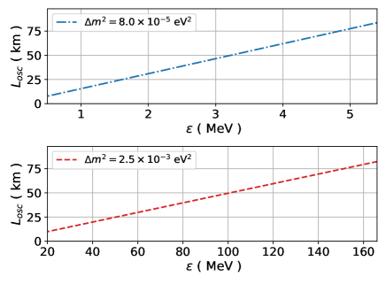
In the flat spacetime approach, the flavour states are considered to be the superposition of the energy eigenstates often having same radial momentum which implies Giunti (2001). Consequently, in the flat spacetime limit i.e. , phase difference (13) reduces to
| (14) |
where is known as the vacuum oscillation length of neutrinos. The vacuum oscillation lengths for different combinations of the parameters and are shown in the FIG. 1.
III.2.2 A missing factor of
We note that the flat spacetime expression of (14) in terms differs by a factor of compared to the analogous expression often stated in many literatures GÓŹDŹ and ROGATKO (2011); Bilenky and Pontecorvo (1978) (however see Bhattacharya et al. (1999)). This difference essentially arises because in those literature one assumes, rather erroneously, that a neutrino follows a null trajectory i.e. . Neutrino being a massive particle, albeit with a very small mass, it follows a timelike trajectory given by (11). This aspect of the neutrino trajectory leads to an additional contribution involving to the phase difference (13, 14).
IV Fermions in curved spacetime
In the previous section, we have considered the neutrinos as relativistic, massive particles that are propagating along the geodesics in a curved spacetime. However, the neutrinos are fermions and are described by the spinor field in the Standard Model. Therefore, in order to describe the propagation of neutrinos in a curved spacetime, it is imperative to employ a generally covariant action for the fermions.
IV.1 Dirac equation
We consider the neutrino to be a Dirac spinor here. In the Fock-Weyl formulation, the dynamics of a free fermion in a curved spacetime is governed by the action Weyl (1929); V (1929)
| (15) |
where is known as the Dirac adjoint and being the mass of the fermion. Here are the components of the tetrads which form a basis for the local tangent space and relates it to the global coordinates such that where . The spin covariant derivative is given by and after imposing the compatibility conditions for tetrads, i.e. we get the spin connection explicitly as
| (16) |
where are the Christoffel connections and are the standard Dirac matrices in Minkowski spacetime satisfying the Clifford algebra such that and for spatial indices . The conserved 4-current corresponding to the action (15) is which satisfies .
The generally covariant field equation for the spinor field i.e. , can also be expressed as
| (17) |
where is summed over the spatial indices. The form of the field equation (17) resembles a quantum mechanical evolution equation with being the Hamiltonian operator. However, in a curved spacetime the operator may not hermitian in general Parker (1980).
IV.2 Dirac equation inside a spherical star
In order to reduce the Dirac equation (17) into a form which is directly applicable for a spherical star, we need to choose the appropriate tetrads and then compute the corresponding spin connections.
IV.2.1 Tetrads and spin connections
By making a diagonal ansatz, the non-vanishing tetrad components corresponding to the metric (1) can be expressed as
| (18) |
Similarly, the non-zero components of the inverse tetrad are
| (19) |
Consequently, the spin-connections (16) associated with the spherically symmetric metric (1) become
| (20) |
and
| (21) |
Here we have used the representation of Dirac matrices given by
| (22) |
where for are the Pauli matrices.
IV.2.2 Energy eigenvalues
In order to arrive at the particle description of neutrinos from the field equation (17), we need to ensure the associated Hamiltonian is hermitian. For a stationary metric, such as the spherically symmetric metric being considered here, the Hamiltonian can be made hermitian Huang and Parker (2009); de Oliveira and Schmidt (2019) by using the inner product defined in the curved spacetime. Consequently, one can associate the quantum-mechanical probability interpretation with the spinor .
We note that the spin connections (20, 21) satisfy , and . Further, and are non-vanishing even in the Minkowski limit due to the usage of spherical polar coordinates. Therefore, to ensure hermiticity, we may define as the hermitian Hamiltonian for describing the propagation of neutrinos. Ideally, one should consider a wave-packet for describing propagation of neutrino as a particle. For simplicity here we consider the neutrinos to be moving radially with the radial wave-vector such that . The corresponding equation of motion for the mode can then be expressed as
| (23) |
where is the Hamiltonian for the mode. By diagonalising the mode Hamiltonian matrix we can find the corresponding energy eigenvalues as
| (24) |
where negative eigenvalues correspond to the anti-particles. We note that if we identify the radial wave co-vector with the radial co-momentum , the energy eigenvalues have the same form as the conserved energy (6). Besides, these modes satisfy the usual quantum mechanical time evolution equation (23). In other words, these modes follow exactly the same properties as the propagating relativistic quantum particles as studied in the Section III. Henceforth, for brevity of notation we shall drop the sub-script while describing these modes.
IV.2.3 Transition probability of neutrinos
Let us consider a beam of electron neutrinos which is produced at a source located at . So the transition probability of an initially electron neutrino state transforming into a non-electron neutrino state state after propagating through a baseline can be expressed as
| (25) |
where is the phase difference (10) arising due to the propagation and the angle refers to the vacuum mixing angle (8).
IV.3 MSW Effects
In the study of solar neutrinos, one includes the effect of matter interaction by considering the elastic forward scattering (refraction) of neutrinos Mikheev and Smirnov (1987); Smirnov (2005, 2003). This effect is known as the Mikheyev-Smirnov-Wolfenstein (MSW) effect. In the Glashow-Salam-Weinberg theory of electro-weak interactions Weinberg (1967), the neutrinos interact via 4-fermion current-current interaction terms Wolfenstein (1975) having both the neutral current and the charged current. However the neutral current interaction, arising due to the interaction with the nucleons, is ‘flavour blind’ Sawyer (1975) and consequently it leads to an overall phase without impacting the neutrino oscillations.
IV.3.1 Charged current interaction
On the other hand, the charged current interaction affects the neutrino oscillations and is described by the action
| (26) |
where is the Fermi coupling constant and is the charged current due to the electron field . In a spherically symmetric, static spacetime, we may approximate the background electron current as where is the electron number density. Consequently, the interaction Lagrangian density, defined as , reduces to
| (27) |
where the projection operator is and we have used the fact . We note that does not contain any explicit dependence on the spacetime metric. However, the metric dependence is contained in the term .
The Dirac field equations for the neutrinos having masses and can then be expressed as
| (28) |
where , , with . Here and are the mode Hamiltonians, defined in the equation (23) for the masses and respectively. The presence of the projector in the equation (28) signifies the fact that the electroweak sector in the Standard Model is described by gauge symmetry group where only the left-handed neutrino states can interact with the background electrons.
IV.3.2 Energy eigenvalues
Assuming to be time-independent, we can diagonalise the equations (28) to obtain the energy eigenvalues in the presence of matter interaction. For the modes having radial co-momentum , we can express the interacting energy eigenvalues in terms of the non-interacting energy eigenvalues , as
| (29) |
where and . The energy gap in the presence of matter interaction can be expressed as . Here we may define a characteristic number density for the electrons which signifies the strength of the interaction and it allows one to express as
| (30) |
In the flat spacetime limit , the equations (29, 30), become identical to those derived by Wolfenstein Wolfenstein (1978). Further, if we turn off the matter interaction by setting , then and the energy eigenvalues and reduce to the non-interacting eigenvalues and as expected.
IV.3.3 Matter mixing angle
Using the equation (8), we can express the time-evolution equation (28) for the neutrino flavour states in the presence of matter interaction with a constant potential , as
| (31) |
where . The angle is known as the matter mixing angle and it is defined through the relations
| (32) |
Consequently, in the presence of matter interaction, we may express the neutrino flavour states as the superposition of the energy eigenstates given by
| (33) |
where and are the energy eigenstates with the eigenvalues and respectively.
IV.3.4 Adiabatic approximation
The matter mixing angle together with the equation (31) is strictly valid for a constant potential , requiring constant (matter) electron density as well as a constant metric function . However, these equations may still be used for a slowly varying density medium if the variation is subject to the adiabatic condition Mikheyev and Smirnov (1985); Messiah (1986), given by
| (34) |
If the condition (34) is satisfied then the transitions between the energy eigenstates can be neglected and the energy eigenstates can be considered to be propagating independently of each other. It also requires that the matter interaction be perturbative in nature i.e. . Consequently, we may approximate the trajectories of neutrinos inside a matter medium to follow the geodesics, implying the eigenvalues and to remain conserved during the propagation.
IV.3.5 Applicability of matter mixing for a neutron star
In view of considerable uncertainties in our understanding of the dense nuclear matter, it is an open issue whether the interaction (26) considered in the study of solar neutrinos would remain to be the most relevant interaction even for the neutron stars. If it is so then from the FIG. 1, we note that at the relevant scale for the neutron star radius, eV. It corresponds to the characteristic density being fm-3. On the other hand, inside a neutron star the scale of electron density being fm-3 corresponds to eV. Therefore, the parameter inside a typical neutron star becomes . Further, if we assume then the adiabatic approximation ratio becomes . It shows that adiabatic condition (34) could be satisfied inside a typical neutron star.
IV.3.6 Transition probability of neutrinos
In the presence of matter interaction, the transition probability of an initially electron neutrino state transforming into a non-electron neutrino state after propagating through a baseline in a slowly varying matter density medium where the adiabatic condition (34) holds, is given by Smirnov (2019)
| (35) | |||||
We note that in a constant density medium where or in the vacuum where , the transition probability (35) reduces to the expression (25) as expected.
V Neutron Stars
Inside a neutron star under -equilibrium, the constituent nucleons go through the processes of -decay and inverse -decay. These processes are known as the Urca processes and they produce neutrinos or anti-neutrinos of electron flavour only. One such process, known as the direct Urca process, leads to generation of electron-flavour neutrinos through the process and . These neutrinos then propagate out of the neutron stars carrying away energy. Consequently these neutrino generation processes form a dominant cooling mechanism for the neutron stars. There are considerable uncertainties in understanding the efficiencies of different Urca processes. However, each of these processes primarily leads to the generation of only electron-flavour neutrinos. This particular aspect would play an important role for using the neutrino oscillations as a probe for constraining the nuclear matter EOS of the neutron stars.
V.1 Flavour composition of emitted neutrinos
As discussed before, the Urca processes inside a neutron star are known to produce only electron-flavour of neutrinos. However, a certain fraction of these electron neutrinos would transform into non-electron neutrinos due to the flavour oscillations during their propagation. The flavour composition of emitted neutrinos depends on the phase difference between the corresponding energy eigenstates (13). Besides, the probability of direct Urca process occurring near the stellar core is much higher Brown et al. (2018). Therefore, for simplicity, we shall assume these electron-neutrinos are predominantly produced near the core of the star. So the phase difference near the stellar surface when the neutrinos are propagating out of the neutron star, can be expressed as
| (36) |
where
| (37) |
If we use the approximation then the phase difference becomes
| (38) |
In the flat spacetime limit i.e. , , the factor . However, in a curved spacetime the factor can be different from depending on the interior metric solution of the star. In summary, the flavour composition of emitted neutrinos from a neutron star near the stellar surface carry information about the interior spacetime metric. This aspect can be used to put constraints on the possible nuclear matter EOS of a given neutron star.
V.2 Extraction of the factor
V.2.1 Vacuum or constant electron density medium
From the equations (25, 38) we note that in principle if we could observe the flavour composition of emitted neutrinos at two different energy scales say and then we could eliminate the mixing angle from the determination of the factor . In particular, we could express
| (39) |
where and for . In other words, for a given neutron star, one could extract the factor from the determination of the ratio of normalized counts of non-electron neutrinos emitted at two different energy scales near the stellar surface.
V.2.2 Varying electron density medium
Similar to the case of vacuum or constant density medium, one could extract the factor even for a medium where density variations obey the adiabatic approximation. However, in this case one would need to observe the flavour composition of emitted neutrinos for at least three different energy scales say , , and . Consequently, we could eliminate the mixing angle from the determination of the factor as
| (40) |
where for . Here we have neglected the terms which are for large values of . As earlier, for a given neutron star, one could extract the factor from the determination of the ratio of the normalized differential counts of non-electron neutrinos emitted near the stellar surface by considering at least three different energy scales.
V.3 Constraint on the equation of states
We have already argued that the flavour composition of emitted neutrinos near the stellar surface depends, apart from the properties of neutrinos and the stellar radius , also on the factor which in turns depends on the interior metric solution. Therefore, the values of the factor estimated from the observations can be contrasted with the values which are computed for different possible nuclear matter EOS of a given neutron star.
V.3.1 Models of equation of states
In order to elucidate the usage of neutrino oscillations as a probe, in this section we compute the factor by considering three different choices of the nuclear matter EOS for a neutron star. The first EOS that we choose is the standard polytropic EOS of the form . For convenience, here we consider a parametric form for the energy density as where may be viewed as the nucleon number density and being the average mass of the nucleons. Here we choose to be the mass of the neutrons. Further, we introduce a constant so that the term is a dimensionless quantity. Therefore, we can express the energy density and the pressure corresponding to the polytropic EOS in a parametric form as
| (41) |
where and are referred to as the polytropic index and the polytropic coefficient respectively.
Additionally, we consider two variants of the nuclear matter EOS described by the model of nuclear interaction and computed using thermal quantum field theory in a curved spacetime Hossain and Mandal (2021b); Hossain and Mandal (2022). The first variant of the equation of state is computed in a flat spacetime and we refer to it as the flat EOS. The second variant of the equation of state is computed by considering the curved spacetime of a given neutron star which we refer to as the curved EOS. For both these model EOS, the nuclear matter is composed of neutrons, protons and electrons in -equilibrium and interaction between the baryons are mediated by the and mesons.
V.3.2 Neutron star with mass
Let us consider a neutron star having mass and radius km. Such a neutron star can be obtained from multiple EOS with different values of their parameters. A set of parameters that lead to the given neutron star due to the polytropic EOS, the flat EOS and the curved EOS are tabulated as ‘Set 1’ in the TABLE LABEL:table:Parameters14.
| EOS | Set | Parameters | |
|---|---|---|---|
| (fm-3) | |||
| Polytropic | 1 | 1.652 | |
| flat | 1 | 0.684 | |
| curved | 1 | 0.615 | |
| Polytropic | 2 | 1.707 | |
| flat | 2 | 0.666 | |
| curved | 2 | 0.613 |
The resultant mass, radius and the factor are tabulated in the TABLE LABEL:table:MassRadiusGamma14.
| EOS | Set | |||||
|---|---|---|---|---|---|---|
| Polytropic | 1 | 1.40 | 11.50 | 0.767 | 1.885 | 1.326 |
| flat | 1 | 1.40 | 11.50 | 0.776 | 1.695 | 1.236 |
| curved | 1 | 1.40 | 11.50 | 0.783 | 1.550 | 1.167 |
| Polytropic | 2 | 1.41 | 11.42 | 0.763 | 1.911 | 1.337 |
| flat | 2 | 1.39 | 11.55 | 0.779 | 1.679 | 1.229 |
| curved | 2 | 1.39 | 11.48 | 0.785 | 1.546 | 1.165 |
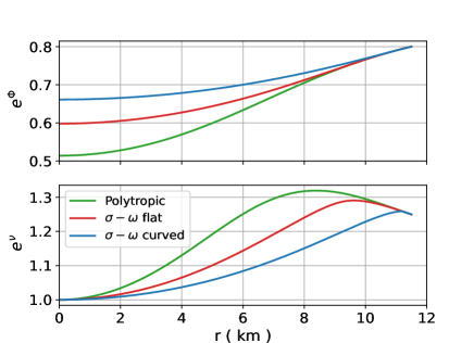
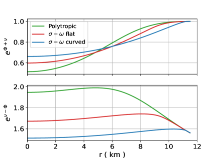
Although all 3 different EOS lead to a neutron star having the same mass and radius hence the same compactness but the resultant factor differs from each other due to having different interior metric solutions. The radial variations of the metric solutions, for the Set 1 parameters, are plotted in the FIG. 2 whereas the radial variations of integrand and are plotted in the FIG. 3.
As an illustration, we note that if neutrinos are observed at two different energies say MeV and MeV then for eV2 along with the parameters given in the Set 1 of the TABLE LABEL:table:MassRadiusGamma14, the probability ratio (39) takes the values , and for the polytropic, the flat, and the curved EOS respectively. In principle, such a ratio could be compared with the observations. Additionally, from the TABLE LABEL:table:MassRadiusGamma14, we note that for a specific EOS, a small variation of the mass and the radius lead only to a small variation of the factor .
V.3.3 Neutron star with mass
Let us consider another example of a neutron star having mass and radius km. A chosen set of parameters that lead to the given neutron star due to the polytropic EOS, the flat EOS and the curved EOS are tabulated in the TABLE LABEL:table:Parameters20.
| EOS | (fm-3) | Parameter set |
|---|---|---|
| Polytropic | 1.319 | |
| flat | 0.640 | |
| curved | 1.244 |
The resultant mass, radius and the factor is tabulated in the TABLE LABEL:table:MassRadiusGamma20.
| EOS | |||||
|---|---|---|---|---|---|
| (km) | |||||
| Polytropic | 2.00 | 12.50 | 0.669 | 2.416 | 1.542 |
| flat | 2.00 | 12.50 | 0.685 | 2.073 | 1.379 |
| curved | 2.00 | 12.50 | 0.685 | 2.071 | 1.378 |
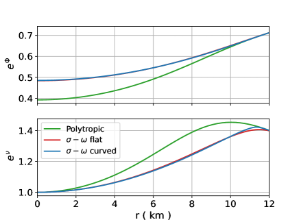
Unlike the previous example, here we note that despite having different parameter sets, the flat EOS and the curved EOS cannot be well distinguished from comparison of the factor . However, one can still differentiate between the polytropic EOS and the EOS. This aspect can also be seen from the radial variation of the metric functions in the FIG. 4. This example also shows the limitation of using neutrino oscillations for differentiating EOS of neutron stars. Clearly, there are regions in the parameter space where the method described here may not be able to distinguish different possible nuclear matter EOS.
VI Discussions
In summary, we have shown that the phenomena of neutrino oscillations and the flavour mixing could be used as a probe for differentiating possible equation of states of nuclear matter of a neutron star if one could determine the flavour composition of emitted neutrinos near the stellar surface. Such possible usage of neutrino oscillations stems from the fact that the transition probabilities among different neutrino flavours are dependent on the interior stellar metric through which these neutrinos propagate out from the stellar interior. On the other hand, different equation of states of nuclear matter implies different interior metric solutions even for a neutron star having the same mass and radius. The method described here could work even for an isolated neutron star where constraining its nuclear matter equation of states through the tidal deformation method is not possible.
Nevertheless, it is acknowledged that the direct determination of the flavour composition of emitted neutrinos near the stellar surface would be a challenging task for a distant observer and one may have to look for possible indirect methods. Observational data indicates that the neutron stars have a thin layer of atmosphere Ho and Heinke (2009); Zavlin and Pavlov (2002). An indirect method for determination of the flavour composition could be to look for possible signatures emanating from the interactions of non-electron neutrinos with the stellar atmosphere.
In our analysis, we have assumed that the neutrinos are described by the Dirac spinor. However, there exists a debate in the literature whether the neutrinos should be considered as Majorana fermions. Besides, we have considered only the left-handed neutrinos to undergo interactions with the background electron density.
Acknowledgements.
SB thanks IISER Kolkata for supporting this work through a masters fellowship. GMH acknowledges support from the grant no. MTR/2021/000209 of the SERB, Government of India.References
- Evans (2013) J. Evans, The MINOS experiment: results and prospects (2013), eprint arXiv:1307.0721.
- Bellerive et al. (2016) A. Bellerive, J. Klein, A. McDonald, A. Noble, and A. Poon, Nuclear Physics B 908, 30–51 (2016).
- Abe et al. (2023) K. Abe, N. Akhlaq, R. Akutsu, H. Alarakia-Charles, A. Ali, Y. I. A. Hakim, S. A. Monsalve, C. Alt, C. Andreopoulos, M. Antonova, et al. (2023), eprint arXiv:2305.09916.
- Abe et al. (2008) S. Abe, T. Ebihara, S. Enomoto, K. Furuno, Y. Gando, K. Ichimura, H. Ikeda, K. Inoue, Y. Kibe, Y. Kishimoto, et al. (The KamLAND Collaboration), Phys. Rev. Lett. 100, 221803 (2008).
- Fukuda et al. (1998) Y. Fukuda, T. Hayakawa, E. Ichihara, K. Inoue, K. Ishihara, H. Ishino, Y. Itow, T. Kajita, J. Kameda, S. Kasuga, et al. (Super-Kamiokande Collaboration), Phys. Rev. Lett. 81, 1562 (1998).
- Wester et al. (2024) T. Wester, K. Abe, C. Bronner, Y. Hayato, K. Hiraide, K. Hosokawa, K. Ieki, M. Ikeda, J. Kameda, Y. Kanemura, et al., Physical Review D 109 (2024).
- Acero et al. (2022) M. Acero, P. Adamson, L. Aliaga, N. Anfimov, A. Antoshkin, E. Arrieta-Diaz, L. Asquith, A. Aurisano, A. Back, C. Backhouse, et al., Physical Review D 106 (2022).
- Abbasi et al. (2023) R. Abbasi, M. Ackermann, J. Adams, S. Agarwalla, J. Aguilar, M. Ahlers, J. Alameddine, N. Amin, K. Andeen, G. Anton, et al., Physical Review D 108 (2023).
- Ahluwalia and Burgard (1996a) D. V. Ahluwalia and C. Burgard, General Relativity and Gravitation 28, 1161–1170 (1996a).
- Ahluwalia and Burgard (1996b) D. V. Ahluwalia and C. Burgard (1996b), eprint gr-qc/9606031.
- Grossman and Lipkin (1997) Y. Grossman and H. J. Lipkin, Physical Review D 55, 2760–2767 (1997).
- Píriz et al. (1996) D. Píriz, M. Roy, and J. Wudka, Physical Review D 54, 1587–1599 (1996).
- Cardall and Fuller (1997) C. Y. Cardall and G. M. Fuller, Physical Review D 55, 7960–7966 (1997).
- Bhattacharya et al. (1999) T. Bhattacharya, S. Habib, and E. Mottola, Phys. Rev. D 59, 067301 (1999).
- Maiwa and Naka (2004) H. Maiwa and S. Naka (2004), eprint arXiv:hep-ph/0401143.
- GÓŹDŹ and ROGATKO (2011) M. GÓŹDŹ and M. ROGATKO, International Journal of Modern Physics E 20, 507–513 (2011).
- Zhang and Li (2016) Y.-H. Zhang and X.-Q. Li, Nucl. Phys. B 911, 563 (2016), eprint arXiv:1606.05960.
- Mandal (2021) S. Mandal, Nuclear Physics B 965, 115338 (2021).
- Capolupo et al. (2023) A. Capolupo, A. Quaranta, and R. Serao, Symmetry 15, 807 (2023).
- Mikheev and Smirnov (1987) S. P. Mikheev and A. Y. Smirnov, Sov. Phys. JETP 65, 230 (1987).
- Smirnov (2005) A. Y. Smirnov, Physica Scripta T121, 57–64 (2005).
- Smirnov (2003) A. Y. Smirnov (2003), eprint arXiv:hep-ph/0305106.
- Hartle (1967) J. B. Hartle, The Astrophysical Journal 150, 1005 (1967).
- Hartle and Thorne (1968) J. B. Hartle and K. S. Thorne, The Astrophysical Journal 153, 807 (1968).
- Hossain and Mandal (2024) G. M. Hossain and S. Mandal, Journal of Cosmology and Astroparticle Physics 2024, 063 (2024).
- Hossain and Mandal (2021a) G. M. Hossain and S. Mandal, Journal of Cosmology and Astroparticle Physics 2021, 026 (2021a).
- Tolman (1939) R. C. Tolman, Phys. Rev. 55, 364 (1939).
- Oppenheimer and Volkoff (1939) J. R. Oppenheimer and G. M. Volkoff, Physical Review 55, 374 (1939).
- Gribov and Pontecorvo (1969) V. Gribov and B. Pontecorvo, Physics Letters B 28, 493 (1969).
- Maki et al. (1962) Z. Maki, M. Nakagawa, and S. Sakata, Progress of Theoretical Physics 28, 870 (1962).
- Giunti (2001) C. Giunti, Modern Physics Letters A 16, 2363–2369 (2001).
- Bilenky and Pontecorvo (1978) S. M. Bilenky and B. Pontecorvo, Phys. Rept. 41, 225 (1978).
- Weyl (1929) H. Weyl, Z. Phys. 56, 330 (1929).
- V (1929) F. V, Z. Phys. 57, 261 (1929).
- Parker (1980) L. Parker, Phys. Rev. D 22, 1922 (1980).
- Huang and Parker (2009) X. Huang and L. Parker, Physical Review D 79 (2009).
- de Oliveira and Schmidt (2019) M. D. de Oliveira and A. G. M. Schmidt, Annals Phys. 401, 21 (2019).
- Weinberg (1967) S. Weinberg, Phys. Rev. Lett. 19, 1264 (1967).
- Wolfenstein (1975) L. Wolfenstein, Nuclear Physics B 91, 95 (1975).
- Sawyer (1975) R. F. Sawyer, Phys. Rev. D 11, 2740 (1975).
- Wolfenstein (1978) L. Wolfenstein, Phys. Rev. D 17, 2369 (1978).
- Mikheyev and Smirnov (1985) S. P. Mikheyev and A. Y. Smirnov, Sov. J. Nucl. Phys. 42, 913 (1985).
- Messiah (1986) A. Messiah, Preprint Saclay PhT/86-46 p. 373 (1986).
- Smirnov (2019) A. Y. Smirnov (2019), eprint arXiv:1901.11473.
- Brown et al. (2018) E. F. Brown, A. Cumming, F. J. Fattoyev, C. Horowitz, D. Page, and S. Reddy, Physical Review Letters 120 (2018).
- Hossain and Mandal (2021b) G. M. Hossain and S. Mandal, Physical Review D 104, 123005 (2021b).
- Hossain and Mandal (2022) G. M. Hossain and S. Mandal, Reviews of Modern Plasma Physics 6, 1 (2022).
- Ho and Heinke (2009) W. C. G. Ho and C. O. Heinke, Nature (London) 462, 71 (2009).
- Zavlin and Pavlov (2002) V. E. Zavlin and G. G. Pavlov (2002), eprint arXiv:astro-ph/0206025.