A Singular Integral for a Simplified Clairaut Equation

Abstract

This expository article makes a connection between Euler’s homogeneous function theorem and a Lagrange integral for a simplified version of the Clairaut Equation. After describing both solutions in detail, we prove a new result, that the Lagrange solution is strictly more general than Euler’s solution. This is shown using a few examples which substitute Euler’s homogeneous function with a more general surface. The first rather complicated example is based directly on Goursat’s definition of a general integral, while the subsequent simpler examples are based on a suitably expanded notion of the general integral. These new examples, and the expanded notion of the general integral may be of interest. We aim to present these classical PDE concepts to readers with a basic knowledge of multivariable calculus.

1 Introduction

We look at general solutions to the following PDE (Partial Differential Equation):

$$x\frac{\partial z}{\partial x}+y\frac{\partial z}{\partial y}=z.$$ (1)

One family of solutions to this equation is provided by Euler’s homogeneous function theorem. The theorem starts with a function $f(x,y)$ such that $f(sx,sy)=s^{n}f(x,y)$, in other words, a homogenous function of order $n$. The theorem states that for such a function,

$$x\frac{\partial f}{\partial x}+y\frac{\partial f}{\partial y}=nf(x,y).$$ (2)

More specifically, if we set $n=1$ we have the following:

$$x\frac{\partial f}{\partial x}+y\frac{\partial f}{\partial y}=f(x,y).$$ (3)

This looks remarkably similar to the simplified Clairaut equation (1) where $z$ has been replaced by $f(x,y)$. It is easy to verify that functions $z=f(x,y)$ where $f$ is of order $n=1$ are valid solutions of equation (1). Some sources [Wik] go further and state a partial converse that the most general solution to equation (2) is a homogenous function $f$ of order $n$, or in the case of (3), a homogeneous function $f$ of order $1$.

We note an important distinction here, that the two equations (1) and (3) look similiar, but they are not the same, and are not equivalent. In particular, we may have relations $f(x,y,z)=0$ that are not representable as a function $z=f(x,y)$ and still obey the restricted Clairaut equation (1), for instance the surface $z^{2}=x^{2}+y^{2}$, a double cone. In this paper we refer to such a surface suggestively as a homogeneous surface since the associated polynomial, in this case $z^{2}-x^{2}-y^{2}$, is homogeneous.

Another source of confusion is Euler’s principle that the integration of a PDE of order $n$ is complete if the integral contains $n$ arbitrary functions. One might argue that the homogenous solution $z=f(x,y)$ contains such an arbitrary function $f$, and thus assume that it is the most general solution possible. This is not true based on various examples we show including the double cone above, $z^{2}=x^{2}+y^{2}$. It is possible that homogeneous functions cannot be regarded as arbitrary, but it is still unclear how to apply the principle suitably in our context, and whether there is a version that applies to relations $f(x,y,z)=0$ and not just to functions $z=f(x,y)$.

In order to introduce Lagrange’s solution, we start with the most obvious solution to (1), namely $z=ax+by$ with arbitrary constants $a$, $b$. A little more thought may suggest some more solutions like $\sqrt{xy}$ or even $x^{\alpha}y^{1-\alpha}$ all of which are within the ambit of Euler’s homogeneous solution. The surprising fact is that the simplest of these solutions, namely $z=ax+by$, can be used to generate all the other solutions including Euler’s in an algorithmic manner, and this is the gist of Lagrange’s solution.

The main claim in this paper is that the Lagrange integral, which we have only hinted at, and not yet defined, is strictly more general than Euler’s family of homogeneous functions. In particular, the Lagrange integral can be used to derive Euler’s homogeneous functions, and also more general surfaces like the following one which are not in Euler’s functional form $z=f(x,y)$:

$$x^{2}+y^{2}+z^{2}-2xz-2yz=0$$

Our claim and examples appear to be new based on our reading of the literature. Given the subtleties around general solutions to a PDE, these results may hold some pedagogical value, especially the expanded notion of a general integral. The generality claim regarding the Lagrange integral does not contradict Euler’s homogeneous function theorem, though it is at odds with Euler’s principle.

The equation at hand (1) is a special case of the Clairaut equation ([Eva10, p.93]) which is as follows:

$$x\frac{\partial z}{\partial x}+y\frac{\partial z}{\partial y}+k\left(\frac{\partial z}{\partial x},\frac{\partial z}{\partial y}\right)=z.$$ (4)

Clairaut’s equation is one of the simpler nonlinear PDEs and one might see it early on in a PDE book. While Clairaut was a reputed physicist, the motivation for this particular equation appears to have been purely mathematical.

The rest of the paper is organized as follows. The upcoming section covers preliminaries related to the Lagrange solution like complete integral and singular integral, and contrasts these with Euler’s homogeneous solution. The third section contains a simple derivation of Euler’s solution while the fourth is devoted to the Lagrange singular integral including material on envelopes and singular integrals. The fifth section connects Lagrange’s integral to Euler’s solution with some examples, and this is followed by a brief conclusion.

2 Preliminaries

To understand Lagrange’s solution we need a couple of notions which we now describe. First is the notion of a complete integral, which an older text like Goursat defines as a family of integrals $f(x,y,z,a,b)=0$ that involve two arbitrary constants (or parameters) $a$, $b$. Newer texts like [Eva10, p.92] have an equivalent definition where the rank of a certain matrix captures the number of independent parameters and equals two in this case. Next we have the notion of a singular integral which [Eva10, p.95] defines as the envelope of this family of integrals (also [Gou17, p.237]). A third notion is that of a general integral which is a type of complete integral where $b$ is assumed to be a function of $a$, say $b=\phi(a)$ [Gou17, p.238].

The complete integral for equation (4) is known to be $z=ax+by+k(a,b)$ where $a$ and $b$ are arbitrary constants. For the restricted equation with $k=0$, the complete integral is more specifically:

$$z=ax+by.$$ (5)

According to Lagrange (and [Gou17, p.236]), once we have the complete integral, that is, a family of integrals which depends upon two arbitrary parameters $a$ and $b$, we can derive all the other integrals from them by differentiations and eliminations. But it is not clear how to operationalize this idea, and come up with the solutions indicated earlier. It is also unclear how Euler’s homogenous solution relates to this complete integral. The current expository paper is an attempt to describe Goursat’s method of differentiations and eliminations, and to connect these integrals to Euler’s homogenous solution.

The current problem illustrates two different ways of representing a general solution. According to Euler [Eng80], an integral of order $n=1$ is complete if it contains $n=1$ arbitrary functions. In his view, the arbitrary constants in the solution to an ordinary differential equation is taken over by an arbitrary function in the case of partial differential equations. Lagrange on the other hand uses the modern notion of a complete integral requiring two arbitrary constants, say $a$, $b$ and a relation $f(x,y,z,a,b)=0$.

Euler’s homogeneous function theorem seems innocuous, and does not claim to present a general solution to a PDE. On the other hand, Euler’s principle of arbitrary functions feels problematic in our context. A careless application of the principle would suggest that homogeneous solutions are the most general ones for the restricted Clairaut equation. But this conclusion is incorrect, as we have seen. Further study is required to understand what Euler had in mind, and whether in fact, the principle is valid.

In any case, Lagrange’s complete integral seems like an elegant improvement over Euler’s principle of arbitrary functions, and does not suffer from such ambiguities. The Lagrange viewpoint seems well matched with modern ideas in differential geometry, and it is not surprising that it continues to find a place in contemporary PDE textbooks.

A specific goal of this paper is to consider the restricted Clairaut equation (1) and prove that Lagrange’s formulation is strictly more general than Euler’s. Euler’s solutions are of the form $z=f(x,y)$ where $f$ is a homogenous function of degree $1$. The formulation by Lagrange says that all solutions can be found from the complete integral (5) by differentiations and eliminations. In particular, a solution to the equation is not required to be of the form $z=f(x,y)$ where $z$ is a function of $(x,y)$. In fact, we will find that Lagrange’s solution, unlike Euler’s, includes a broader class relations $f(x,y,z)=0$ which may have a one to many relation between $(x,y)$ and $z$.

3 Euler’s Solution

In this section, we will look at a simple and systematic approach to deriving Euler’s solution. We start with a change of variables $X=\ln x$, $Y=\ln y$ and $Z=\ln z$. This can be motivated by the suggestive form $\frac{\partial z}{z}\frac{x}{\partial x}+\frac{\partial z}{a}\frac{y}{\partial y}=1$. With this change of variables, we have the following calculations:

$$\frac{\partial Z}{\partial X}=\frac{\partial Z}{\partial z}\frac{\partial z}{\partial x}\frac{\partial x}{\partial X}=\frac{1}{z}\frac{\partial z}{\partial x}x,$$

$$\frac{\partial Z}{\partial Y}=\frac{\partial Z}{\partial z}\frac{\partial z}{\partial y}\frac{\partial y}{\partial Y}=\frac{1}{z}\frac{\partial z}{\partial y}y.$$

This gives us the following linearized form of the restricted Clairaut equation:

$$\frac{\partial Z}{\partial X}+\frac{\partial Z}{\partial Y}=\frac{x}{z}\frac{\partial z}{\partial x}+\frac{y}{z}\frac{\partial z}{\partial y}=1.$$

The above logarithmic substitutions restrict the domain of validity to be $x>0,y>0,z>0$. A further change of variables is as follows:

$$X=U+V,$$

$$Y=U-V.$$

This gives us

$$\frac{\partial Z}{\partial U} =\frac{\partial Z}{\partial X}\frac{\partial X}{\partial U}+\frac{\partial Z}{\partial Y}\frac{\partial Y}{\partial U}$$

$$=\frac{\partial Z}{\partial X}+\frac{\partial Z}{\partial Y}$$

$$=1.$$

On the other hand,

$$\frac{\partial Z}{\partial V} =\frac{\partial Z}{\partial X}\frac{\partial X}{\partial V}+\frac{\partial Z}{\partial Y}\frac{\partial Y}{\partial V}$$

$$=\frac{\partial Z}{\partial X}-\frac{\partial Z}{\partial Y}.$$

This is a generic identity and does not seem to impose a particular relationship between $Z$ and $V$. Put differently, we can let $Z$ be an arbitrary function of $V$, and the above identity will continue to hold. Further, $Z=h(V)$ satisfies the following equation for $V=\frac{X-Y}{2}$ and $h$, an arbitrary function:

$$\frac{\partial h(V)}{\partial X}+\frac{\partial h(V)}{\partial Y}=\frac{\partial h(V)}{\partial V}\frac{\partial V}{\partial X}+\frac{\partial h(V)}{\partial V}\frac{\partial V}{\partial Y}=h^{\prime}(V)\frac{1}{2}+h^{\prime}(V)\frac{-1}{2}=0.$$

Now $\frac{\partial Z}{\partial U}=1$ has solutions of the form $Z=U+c$ where $c$ is independent of $U$. Combining this with an arbitrary function $h(V)$, we have the following general solution:

$$Z=U+h(V).$$ (6)

The general solution (6) can also be written as:

$$\ln z=\frac{\ln x+\ln y}{2}+h(\frac{\ln x-\ln y}{2}),$$

$$z=\sqrt{xy}\cdot H(\frac{x}{y}).$$

Given that $H$ is arbitrary, other equivalent forms of this solution include $xH(\frac{x}{y})$ and $xH(\frac{y}{x})$ and $yH(\frac{x}{y})$. All these forms represent homogeneous functions of $x$, $y$ of order $n=1$. It is easy to see that the solutions $z=\sqrt{xy}$ and $z=x^{\alpha}y^{1-\alpha}$ can be easily obtained by suitable choices of the $H$ function. We also note that the domain of validity $x>0,y>0$ required by the $\ln$ function matches that of $z=\sqrt{xy}$ and $z=x^{\alpha}y^{1-\alpha}$.

Finally, we note that for the given domain of validity with $x>0$, any homogeneous function $f$ of order $n=1$ can be represented in the form $xH(\frac{y}{x})$. In particular, we have

$$f(x,y)=f\left(x\cdot 1,x\cdot\frac{y}{x}\right)=xf\left(1,\frac{y}{x}\right)=xH\left(\frac{y}{x}\right)$$

where $H(w)=f(1,w)$.

4 The Lagrange Integral

Having looked at Euler’s solution, we now look at Lagrange’s solution in some detail. The ideas elaborated in this section mirror Goursat’s analysis books, [Gou04, p.426] on envelope calculations and [Gou17, p. 236] on details of the complete integral, the general integral, and the singular integral for Clairaut’s equation. These are old references written in a different style, so the ideas require a little unpacking. Once we turn those ideas into calculations, we will see that Euler’s solution can be obtained from the Lagrange complete integral.

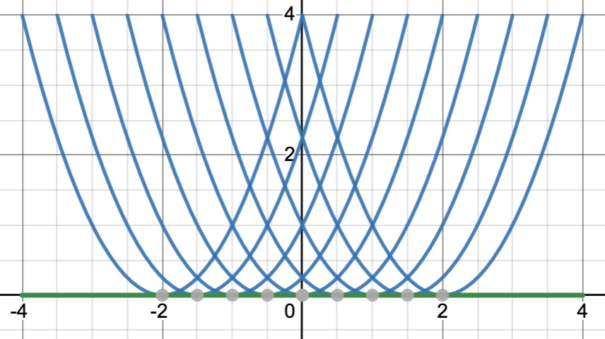
Figure 1: Integrals for $y^{\prime 2}=4y$. The family of parabolas $y=(x+c)^{2}$ is called the complete integral, and each member of this family satisfies the PDE. A curve tangent to this family of parabolas is the $x$ axis $y=0$, and it is called the singular integral, and it satisfies the PDE as well.

The nature of the singular integral is well explained in [Bri23] which shows a family of solutions to the equation $y^{\prime 2}=4y$. The family of solutions $y=(x+c)^{2}$ contains one arbitrary parameter $c$, and can be regarded as a complete integral to the PDE. The tangent to this family of curves is the $x$ axis $y=0$ (Figure 1) and it is called the singular integral. It is easy to verify that both the complete integral $y=(x+c)^{2}$ and the singular integral $y=0$ satisfy the PDE. In this particular example, the complete integral is a higher order curve (a parabola) compared to the singular integral (a straight line). In the case of the restricted Clairaut equation we will find that the complete integral is a simple family of planes while the singular integral takes on rather complex forms based on the parameters chosen.

In the following two subsections, we first derive an envelope calculation procedure, and then use the envelope procedure to calculate singular integrals for the restricted Clairaut equation.

4.1 A Tangent on Envelopes

We take a slight digression at this point to describe an envelope calculation procedure. This material typically belongs in a class on Curves and Surfaces, or perhaps in a class on Differential Geometry though we find that the topic is often skipped in the curriculum. We briefly review the relevant procedure and its justification for completeness. More details can be found in older texts like [Str61, p.162] or [Gou04, p.426].

We would like note here that this article emphasizes clarity over rigor. For instance, the treatment below follows Goursat in describing an envelope procedure. The procedure makes use of certain differentials ($\delta x,\delta y$) which could be expressed more precisely in the language of differential geometry. But Goursat’s $\delta$ notation provides good intuition, and we have chosen to follow it without further justification.

[Gou04, p.426] suggests the following. Starting with $f(x,y,a)=0$, one considers two curves. One curve $C$ that represents $f(x,y,a)=0$ for a fixed parameter $a$, and the other an envelope $E$ for the entire family of curves $f(x,y,a)=0$ for different values of $a$. The envelope can be expressed in parameteric form where $x$ and $y$ are functions of $a$, say $x=\phi(a)$ and $y=\psi(a)$. Consider differentials $\delta x$ and $\delta y$ proportional to the directional cosines of the tangent to the curve $C$. In other words, the vector ($\delta x$, $\delta y$) points along the tangent to the curve $C$. But the tangent to the curve $C$ is also tangent to the envelope which has derivatives ($\frac{dx}{da}$, $\frac{dy}{da}$). This gives us the following:

$$\frac{\frac{dx}{da}}{\delta x}=\frac{\frac{dy}{da}}{\delta y}$$

When we look at the curve $C$, $a$ is fixed and $f$ is constant, so we can infer the following:

$$df=\frac{\partial f}{\partial x}\delta x+\frac{\partial f}{\partial y}\delta y=0.$$

Combining the above two we have:

$$\frac{\partial f}{\partial x}\frac{dx}{da}+\frac{\partial f}{\partial y}\frac{dy}{da}=0.$$ (7)

This appears to be a neat trick. Using the device of $\delta x$ and $\delta y$, we have obtained an identity that combines properties of the curve ($\frac{\partial f}{\partial x}$, $\frac{\partial f}{\partial y}$) and properties of the envelope ($\frac{dx}{da}$, $\frac{dy}{da}$).

Now, considering the envelope $E$ directly, $x$ and $y$ are functions of $a$, and so one can write the following:

$$\frac{\partial f}{\partial x}\frac{dx}{da}+\frac{\partial f}{\partial y}\frac{dy}{da}+\frac{\partial f}{\partial a}=0.$$ (8)

From the above two equations (7) and (8) one can infer the envelope equation:

$$\frac{\partial f}{\partial a}=0.$$ (9)

Further geometric intuition for this envelope equation is provided in [Gou04, p. 429, Fig. 37] which shows nearby curves from the family, and its relation to (9). As an example of this procedure, consider the following family of curves:

$$ax+by=1.$$

Suppose further that we have a constraint $ab=1$. In this case, we can write:

$$ax+\frac{1}{a}y=1,$$

$$a^{2}x+y=a.$$

Now we set:

$$f(x,y,a)=a^{2}x+y-a=0.$$

Letting $\frac{\partial f}{\partial a}=0$,

$$2ax-1=0,$$

$$a=\frac{1}{2x}.$$

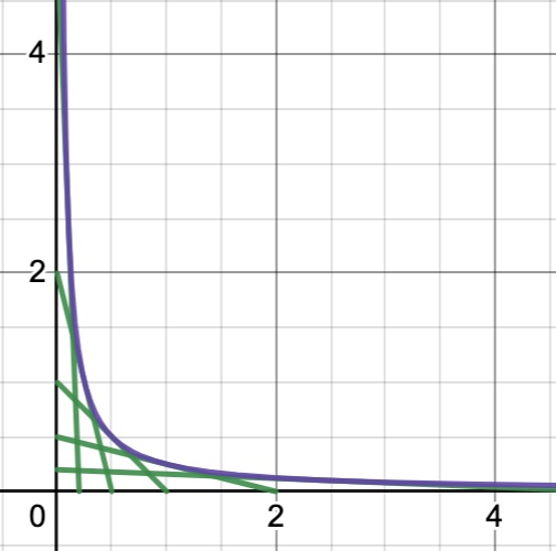
Figure 2: $ax+by=1$ (with $ab=1$), $4xy=1$

Plugging this back into the family of curves we get the envelope $4xy=1$ (Figure 2):

$$\frac{1}{2x}\cdot x+2x\cdot y =1,$$

$$\text{i.e., }4xy =1.$$

4.2 The Singular Integral

We now continue our journey to a general solution given the complete integral (5) and the envelope equation (9). For starters, consider the complete integral $z=ax+by$ where $b$ is a specific function of $a$, say $b=\frac{1}{a}$. This leads to the following:

$$z=ax+\frac{1}{a}y,$$

$$z-ax-\frac{1}{a}y=0.$$

To get a singular integral, one needs to find the envelope of this single parameter family of solutions:

$$f(x,y,z,a)=z-ax-\frac{1}{a}y=0.$$

The envelope is obtained by setting $\frac{\partial f}{\partial a}=0$. That is:

$$-x+\frac{1}{a^{2}}y=0,$$

$$a=\sqrt{\frac{y}{x}}.$$

Using $a=\sqrt{\frac{y}{x}}$, we can now connect the envelope or singular integral back to the earlier solution:

$$z =x\sqrt{\frac{y}{x}}+y\sqrt{\frac{x}{y}}=2\sqrt{xy}.$$

As a simple exercise, one could try to eliminate the constant 2, that is to obtain $z=\sqrt{xy}$. We could also try to find the solution $z=x^{\alpha}y^{1-\alpha}$ in the above manner.

Now to generalize this discussion, let us consider the complete integral $z=ax+by$ where $b=\phi(a)$ is an arbitrary function of $a$. [Gou17, p.237] provides some justification for this relation between $a$ and $b$ based on which we have the following general integral:

$$z=ax+\phi(a)y.$$ (10)

Writing this in canonical form,

$$f(x,y,z,a)=z-ax-\phi(a)y=0.$$

Applying the envelope equation (9), namely $\frac{\partial f}{\partial a}=0$, we obtain the following envelope condition for the above family of planes:

$$x+\phi^{\prime}(a)y=0.$$ (11)

The simplest way to solve (10) and (11) is to write out the solution set in parameteric form as follows:

$$(x,y,z)=(-\phi^{\prime}(a)y,y,-a\phi^{\prime}(a)y+\phi(a)y).$$ (12)

Notice that $y$ appears as a factor in all the coordinates, and that all coordinates are zero when $y=0$. So for non-zero $y$, we could divide the parameterized coordinates by $y$, setting $X=\frac{x}{y}$ and $Z=\frac{z}{y}$, to get the following:

$$(X,Z)=(-\phi^{\prime}(a),-a\phi^{\prime}(a)+\phi(a)).$$ (13)

(13) is a representation of the solution set in a so-called projective space, $\mathbb{R}\mathbb{P}^{2}$. Though we don’t use or define projective spaces in this paper, we mention this representation briefly since it may be a clean and intuitive description of the solution set. Projective representations are useful where homogeneous polynomials are involved with many to many relations $f(x,y,z)=0$ and we will shortly see solutions of this nature.

5 Euler-Lagrange Connection

In this section we first derive Euler’s homogeneous solution from the Lagrange complete integral. We then observe that invertible functions $\phi^{\prime}(a)$ always lead to homogeneous functions as described in Euler’s theorem. To get around this, and find a more general solution, we set $\phi^{\prime}(a)$ to be a non-invertible function and proceed to construct a solution to the restricted Clairaut equation which is not in Euler’s functional form $z=f(x,y)$. Finally, as an antidote to this convoluted example, we show two simple solutions where simplicity is achieved by relaxing the condition $b=\phi(a)$ in a general integral.

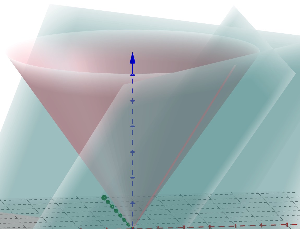
Figure 3: Cone as the envelope of planes

Let us recall the general integral (10), the envelope of a family of planes for a fixed but arbitrary function $\phi$:

$$z=ax+\phi(a)y.$$ (14)

Note that when both $a$ and $\phi$ are fixed, the above represents the equation of a plane of the form $z=\alpha x+\beta y$ for constants $\alpha,\beta$. Now as we vary $a$ keeping $\phi$ fixed we get a family of planes. It may be helpful to keep Figure 3 in mind where three planes from a certain family are shown along with the envelope which is a cone. Also note that points on the envelope satisfy (11) and (14) both of which are homogenous in $(x,y,z)$.

Let the envelope $E$ be tangent to this family of planes at a point $P_{1}=(x_{1},y_{1},z_{1})$. Now, $P_{1}$ obeys (14) for some fixed plane given by (say) $a=a_{1}$. It is clear that $sP_{1}=(sx_{1},sy_{1},sz_{1})$ lies on the same plane since $sP_{1}$ also satisfies (14) with $a=a_{1}$. Further, when $P_{1}$ satisfies the envelope condition (11), the point $sP_{1}$ obeys the envelope condition (11) as well, namely $asx_{1}+\phi^{\prime}(a)sy_{1}=0$. In short, when a point $P=(x,y,z)$ lies on the envelope (satisfying (11) and (14)), the scaled point $sP=(sx,sy,sz)$ lies on the envelope as well, satisfying those two conditions.

If we restrict our solutions to be of the form $z=h(x,y)$, then we also have $sz=h(sx,sy)$ based on the envelope equation for $(sx,sy,sz)$. Multiplying the former by $s$, we have $sz=sh(x,y)$. The two expressions for $sz$ show that $h(sx,sy)=sh(x,y)$. In other $h$ is a homogeneous function, and we have thus derived Euler’s solution from the Lagrange integral. Geometrically, this homogeneous solution may be described as a ruled surface with the radial lines $(sx,sy,sz)$ for fixed $(x,y,z)$ lying on the envelope.

We will now see that invertibility of $\phi^{\prime}(a)$ leads to Euler’s homogeneous functions. We have $\phi^{\prime}(a)=-\frac{x}{y}$ for non-zero $y$. We have already seen that $y=0$ implies $x=0,z=0$, so assuming non-zero $y$ doesn’t lose generality. Now if $\phi^{\prime}(a)$ is invertible, one could say $a=\psi\left(\frac{x}{y}\right)$ where $\psi$ is the negative inverse of $\phi^{\prime}$. Plugging this back to the complete integral, we obtain the following singular integral:

$$z =\psi\left(\frac{x}{y}\right)x+\phi(\psi\left(\frac{x}{y}\right))y.$$

It is clear that the above function is homogeneous of order $n=1$ in $x$, $y$, and is of the form $z=xH\left(\frac{x}{y}\right)$ for a suitable function $H$. Contrariwise, to go beyond Euler’s homogeneous functions we will need to start with $\phi^{\prime}$ that is not invertible.

5.1 Beyond Euler

We have seen that the Lagrange integral yields homogeneous functions when $\phi^{\prime}(a)$ is invertible. We will now construct a function $\phi^{\prime}$ that is non-invertible by design, and use it to derive a more general solution to the restricted Clairaut equation. This example is rather convoluted, and we share this primarily for completeness and to illustrate the possibilities and limitations of a general integral based on $b=\phi(a)$. The next section contains simpler algebraic examples.

Let us define $\phi^{\prime}(a)$ to be the following spline:

$$\phi^{\prime}(a)=\left\{\begin{array}[]{ll}((a-1)^{2}-1)^{2}&\mbox{if }0\leq a\leq 1,\\ 0.5*((a-1)^{2}-1)^{2}+0.5&\mbox{if }1\leq a\leq 2,\\ 0.5*((a-3)^{2}-1)^{2}+0.5&\mbox{if }2\leq a\leq 3,\\ ((a-3)^{2}-1)^{2}&\mbox{if }3\leq a\leq 4,\\ 0&\mbox{o.w.}\end{array}\right.$$ (20)

We have just spliced together four scaled translates of $((a-k)^{2}-1)^{2}$, each of which is a smooth bump-like function between $k-1$ and $k+1$, for $k=1,3$. This gives us a smooth bimodal function that is non-invertible by design. We obtain $\phi(a)$ from $\phi^{\prime}(a)$ by a simple numerical integration. $z$ is computed using $z=-a\phi^{\prime}(a)y+\phi(a)y$ with a fixed value of $y=1$. With $a$ ranging from $0$ to $4$, we obtain a sample set of points $(x,y,z)=(-\phi^{\prime}(a),1,-a\phi^{\prime}(a)+\phi(a))$. Fixing $y=1$ was convenient for calculation, but for visualization it is better to fix $z=1$. This gives us the following set of points instead $(x,y,z)=(\frac{-\phi^{\prime}(a)}{-a\phi^{\prime}(a)+\phi(a)},\frac{1}{-a\phi^{\prime}(a)+\phi(a)},1)$. With this set of points we plot $x$ against $y$.

We now look at two points $P$, $Q$ along a radial line of this cross section as in Figure 4. The non-invertibility of $\phi^{\prime}(a)$ guarantees the existence of two such points. Say $P=(x,y,1)$ and $Q=(\alpha x,\alpha y,1)$ with the $z$ coordinate fixed at $1$ for both points. Notice now, that if $P$ is on the surface, so is $sP$, $\forall s\in\mathbb{R}$. Thus $\alpha P=(\alpha x,\alpha y,\alpha)$ is on the surface along with $(\alpha x,\alpha x,1)$. In particular, we now have two values of $z$, namely $1$, $\alpha$ associated with $(\alpha x,\alpha y)$. In other words, $z$ is not a function of $(x,y)$. The solution is a cone-like 3-D surface but it cannot be expressed as a homogeneous function $z=f(x,y)$. In this sense, we say that Lagrange’s solution is strictly more general than Euler’s solution.

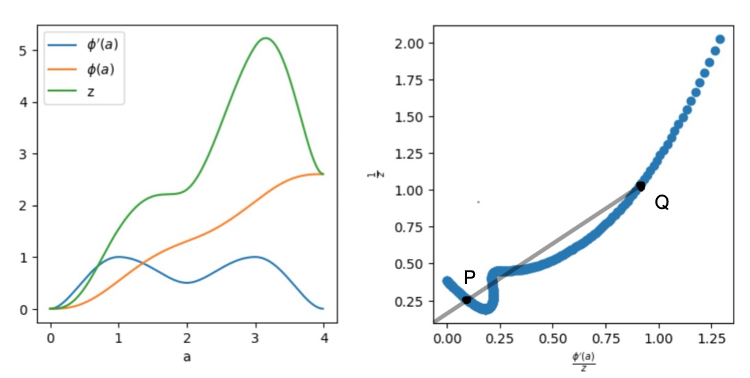
Figure 4: The graphs on the left represent various functions of $a$ starting with an explicitly constructed $\phi^{\prime}(a)$ that is non-invertible by design. $z=-a\phi^{\prime}(a)y+\phi(a)y$. The graph on the right shows a cross section of the surface at $z=1$. $P$ and $Q$ lie on the same radial line, and hence have the same value of $\frac{x}{y}$ in this cross-sectional view. When we project up along the z-axis to get a cone-like surface, this translates to one to many relationship between $(x,y)$ and $z$.

5.2 A Simple Example

The previous example started with $b=\phi(a)$ and constructed a rather complicated singular integral. Here we start by relaxing the notion of a general integral to include relations $\phi(a,b)=0$ rather than just $b=\phi(a)$. This allows us to expand our solution set from homogeneous functions to our suggestively named homogeneous surfaces. Let us consider the relation $(a-1)^{2}+(b-1)^{2}=1$. To obtain the envelope associated with this relation, we can break this up into two parts each of which is functional. Specifically:

$$b=1\pm\sqrt{1-(a-1)^{2}}$$

The two roots represent two functions of $a$. We illustrate our calculation using the positive root since the other one follows the same pattern:

$$ax+(1+\sqrt{1-(a-1)^{2}})y=z$$

$$\implies f(x,y,a)=ax+(1+\sqrt{1-(a-1)^{2}})y-z=0$$

Using the envelope equation $\frac{\partial f}{\partial a}=0$,

$$x+\left(\frac{1}{2\sqrt{1-(a-1)^{2}}}\cdot-2(a-1)\right)y=0$$

$$a=1\pm\frac{x}{\sqrt{x^{2}+y^{2}}}$$

We can now plug this back into the complete integral, again with the positive root for simplicity:

$$\left(1+\frac{x}{\sqrt{x^{2}+y^{2}}}\right)x+\left(1+\frac{y}{\sqrt{x^{2}+y^{2}}}\right)y=z$$

$$x^{2}+y^{2}=\sqrt{x^{2}+y^{2}}(z-x-y)$$

$$z^{2}=2xz+2yz-2xy$$

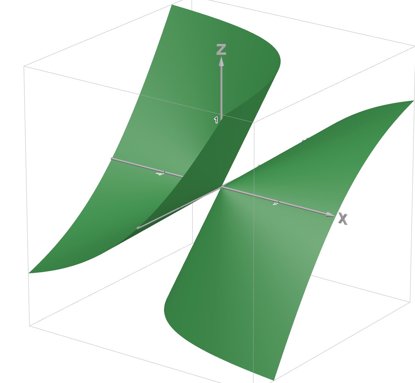
Figure 5: $z^{2}=2xz+2yz-2xy$.

This surface is shown in Figure 5 and accounts for all the positive and negative roots above. We can also verify that the surface $z^{2}=2xz+2yz-2xy$ obeys the restricted Clairaut equation as expected. Thus, our expanded notion of the general integral yields singular integrals which go beyond Euler’s functional form $z=f(x,y)$.

5.3 A Generalized General Integral

We now present another solution where we stretch the notion of a general integral beyond the relation $\phi(a,b)=0$. In this example we start with a singular integral, that is, a solution to the restricted Clairaut equation, and work backwards to find the Lagrange complete integral. A one-line geometric description of this singular integral is that it is a tilted cone, as shown in Figure 6. The axis of the cone is $x=y=z$ and the horizontal $x-y$ cross-sections have radius $r=z$. Algebraically, it can represented in either of these forms:

$$(x-z)^{2}+(y-z)^{2}=z^{2},$$ (21)

$$x^{2}+y^{2}+z^{2}-2xz-2yz=0.$$ (22)

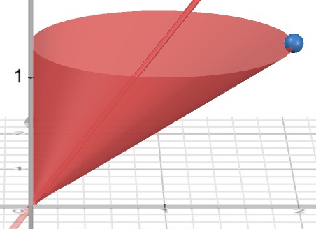
Figure 6: A tilted cone $x^{2}+y^{2}+z^{2}-2xz-2yz=0$ with axis $x=y=z$, and cross-sectional radius $r=z$.

It is easy to verify algebraically or geometrically that this is not of the functional form $z=f(x,y)$. In particular, the surface has two positive values of $z$ for any given $x,y$ in the first or third quadrants. Let us now verify that this cone satisfies the restricted Clairaut equation. The implicit function theorem tells us that $z$ can be regarded as a function of $x,y$ locally. To find this function we represent the surface as a quadratic equation in $z$:

$$z^{2}-z(2x+2y)+(x^{2}+y^{2})=0$$

This gives us the below solution which clearly obeys the restricted Clairaut equation since each of the terms $x$, $y$ and $\sqrt{2xy}$ are known to do so:

$$z=x+y\pm\sqrt{2xy}$$

Here is another proof using directional derivatives that may provide further intuition. For any such cone, consider a point $P$ along with a horizontal, circular cross-section of the tilted cone. The partial derivatives of $z$ can be understood in terms of radial and tangential coordinates within the cross-sectional plane. Since by construction $z=r$, the cross-sectional radius (21), we can assert the following:

$$\frac{\partial z}{\partial r}=1,$$

$$\frac{\partial z}{\partial t}=0$$

That is, $z$ increases as we move radially (or normally), but remains fixed as we move tangentially along the cross-sectional circle. This radial derivative can be used in the following manner assuming the radius makes an angle $\theta$ with the $x$ axis:

$$\frac{\partial z}{\partial x}=\frac{\partial z}{\partial r}\cos{\theta}=\cos{\theta},$$

$$\frac{\partial z}{\partial y}=\frac{\partial z}{\partial r}\sin{\theta}=\sin{\theta}.$$

Plugging these back into the left side of the restricted Clairaut equation:

$$x\frac{\partial z}{\partial x}+y\frac{\partial z}{\partial y} =x\cos{\theta}+y\sin{\theta}$$

$$=x\cdot\frac{x}{\sqrt{x^{2}+y^{2}}}+y\cdot\frac{y}{\sqrt{x^{2}+y^{2}}}$$

$$=\sqrt{x^{2}+y^{2}}$$

$$=z$$

We have now seen three examples of surfaces not covered by Euler’s homogeneous function theorem. Recalling these examples, the first one was based on the notion of a general integral with $b=\phi(a)$ and we proceeded to find a non-invertible $\phi^{\prime}(a)$ in order to build our example. The next example started with the more general form $\phi(a,b)=0$. In the current and last example, the family of planes $ax+by=z$ is contrained by some relation between $a$ and $b$ but we have not put it down in explicit form as $\phi(a,b)=0$. It is easy to see though that the implicit relation between $a$ and $b$ leads to a smooth family of planes. In lieu of a relation $\phi(a,b)=0$ we can obtain a parameterized version of the tangent plane as follows. Consider a point $P$ on the surface of the cone and two tangent lines at that point. The first tangent $L_{1}$ is the same as the line $OP$ connecting $P$ with the origin $O$, and it can be represented as follows:

$$L_{1}=\begin{pmatrix}t+t\cos{\theta}\\ t+t\sin{\theta}\\ t\end{pmatrix}$$

The second line $L_{2}$ is a horizontal tangent at the point $P$ to the circle defined by the horizontal cross-section:

$$L_{2}=\begin{pmatrix}t+t\cos{\theta}-\alpha\sin{\theta}\\ t+t\sin{\theta}+\alpha\cos{\theta}\\ t\end{pmatrix}$$

Since we are looking at tangents to a cone through the origin, the plane defined by $L_{1}$ and $L_{2}$ can be equivalently defined in terms of corresponding tangents $L_{1}^{\prime}$ and $L_{2}^{\prime}$ at a height of $z=1$. In particular, we consider tangents to a point $P^{\prime}$ where $P^{\prime}$ lies on $OP$, and has $z$-coordinate $z=1$. The parameterizations of $L_{1}^{\prime}$ and $L_{2}^{\prime}$ are are a little simpler, and are as follows:

$$L_{1}^{\prime}=\begin{pmatrix}1+\cos{\theta}\\ 1+\sin{\theta}\\ 1\end{pmatrix}\text{ and }L_{2}^{\prime}=\begin{pmatrix}1+\cos{\theta}-\alpha\sin{\theta}\\ 1+\sin{\theta}+\alpha\cos{\theta}\\ 1\end{pmatrix}$$

To parameterize the plane defined by $L_{1}^{\prime}$ and $L_{2}^{\prime}$, we need the perpendicular $N$ to these two lines which is obtained by computing their cross product:

$$N=L_{1}^{\prime}\times L_{2}^{\prime}=\begin{pmatrix}(1+\sin{\theta})-(1+\sin{\theta}+\alpha{\cos{\theta}})\\ -(1+\cos{\theta})+(1+\cos{\theta}-\alpha{\sin{\theta}})\\ (1+\cos{\theta})(1+\sin{\theta}+\alpha\cos{\theta})-(1+\sin{\theta})(1+\cos{\theta}-\alpha\sin{\theta})\end{pmatrix}$$

After simplification, and dividing throughout by common factor $\alpha$ we have:

$$N=\begin{pmatrix}-\cos{\theta}\\ -\sin{\theta}\\ 1+\cos{\theta}+\sin{\theta}\end{pmatrix}$$

We can now reduce this to two dimensions by normalizing the $z$ coordinate to $1$ to obtain $N=(a,b,1)$ where:

$$a=\frac{-\cos{\theta}}{1+\cos{\theta}+\sin{\theta}}$$

$$b=\frac{-\sin{\theta}}{1+\cos{\theta}+\sin{\theta}}$$

One may notice that the above parameterization blows up at $\theta=\pi$ and $\theta=\frac{-\pi}{2}$. Nevertheless, it is visually clear that the family of planes is smooth, and importantly, the envelope is already known to be the tilted cone. An elementary argument is that $\theta=\pi$ corresponds to the plane $x=0$. In particular, $ax+by=z$ can be rewritten at $x+\frac{b}{a}y=\frac{z}{a}$ which devolves to $x=0$ as $a\to\infty$. Similarly, $\theta=\frac{-\pi}{2}$ corresponds to the plane $y=0$ as $b\to\infty$. But this easy way of explaining away singularities may not always work, or it may require further justification, and pull us towards ideas like local charts. Another approach to establish smoothness of the relationship is to eliminate $\theta$ from the above equations. We refrain from doing so for the sake of argument, as it may be difficult to do in the general case. We now have a smooth parameterized family of planes where the relation between $a$ and $b$ is not shown in the explicit form $\phi(a,b)=0$, and yet this family of planes yields a valid singular integral, namely the tilted cone.

We now proceed to connect the singular integrals described in this section back to Goursat’s general integral. In defining the general integral, Goursat [Gou17, p.239] states that we must choose an arbitrary relation between $a$ and $b$, say $b=\phi(a)$ and proceeds to use this last functional form. It is interesting that Goursat restricted his discussion to the simpler functional form $b=\phi(a)$ for his general integral instead of the more general form $\phi(a,b)=0$. Our explanation for this is that the use of a general relation like $\phi(a,b)=0$ introduces difficult questions around the notion of smooth surfaces and smooth families of planes. Our earlier example in this section was restricted to a specific relation $(a-1)^{2}+(b-1)^{2}=1$ where we avoided this problem by overlaying two functions. But speaking more generally of parameterized family of planes, these notions of smoothness may be difficult to define without anticipating the modern theory of manifolds. Goursat may have deftly skirted these problems in his presentation. A general relation between $a$ and $b$ can extend beyond an explicit form such as $\phi(a,b)=0$ to smooth surfaces patched together like splines or manifolds. We could call the resultant family of planes a generalized general integral and believe that it captures Lagrange’s idea more completely.

One may ask if the Lagrange singular integral is the most general one possible, especially in the light of modern differential geometry. This seems like a reasonable proposition for the restricted Clairaut equation, since the Lagrange complete integral is just a smooth collection of tangent planes. One only needs to show that any tangent plane necessarily goes through the origin (so it is of the form $ax+by=z$), but we will not enter into this discussion.

6 Conclusion

The restricted Clairaut equation provides a good pedagogical platform to discuss classical PDE ideas like the complete integral, the singular integral and the general integral. We exhibited a purely algebraic method to arrive at Euler’s homogeneous solution. We then described the idea of a singular integral, and built one using an envelope construction procedure. Finally we proved that the Lagrange singular integral is strictly more general than Euler’s homogenous solution based on some examples. These examples, and the expanded notion of a general integral appear to be new. Given the difficulties in articulating a general solution, and some ambiguity in Euler’s principle of arbitrary functions, we believe these examples may be of interest.

Acknowledgement.

We would like to thank Prof. Rajaram Nithyananda for suggesting the elegant $X=\ln x$ solution and Dr. Gobinda Sau for helpful feedback on this paper.

References

- [Gou04] Edouard Goursat “Derivatives and Integrals” 1.1, Course on Mathematical Analysis Dover Publications, 1904
- [Gou17] Edouard Goursat “Differential Equations” 2.2, Course on Mathematical Analysis Dover Publications, 1917
- [Str61] Dirk J Struik “Lectures on Classical Differential Geometry” Dover Publications, 1961
- [Eng80] S B Engelsman “Lagrange’s early contributions to the theory of first-order partial differential equations” In Historia Mathematica Elsevier, 1980
- [Eva10] Lawrence C Evans “Partial differential equations” American Mathematical Soc., 2010
- [Bri23] Brittanica “Singular Solution”, 2023 URL: https://www.britannica.com/science/singular-solution
- [Wik] Wikipedia “Homogeneous Function” URL: https://en.wikipedia.org/wiki/Homogeneous_function