Evaluation of post-processing pipelines for in vivo ³¹P MR imaging

1 Abstract

BACKGROUND: Low SNR is a persistent problem in X-nuclei imaging because of lower, gyromagnetic ratios and natural abundance as compared to hydrogen. Techniques to combat this is for example, high field MRI, multiple coil acquisitions, and denoising methods.

PURPOSE: The purpose is to evaluate well established methods, such as Kaiser-Bessel regridding, NUFFT, adaptive coil combination, whitened-SVD, compress sensing, and MP-PCA on in vivo phosphor data. To establish which method is optimal under different circumstances for phosphor-GRE and bSSFP-like MRF imaging.

SUBJECTS: 2 males, aged 18 and 45 years participated in the study, along with a 31-P phantom.

SEQUENCE: 7T/stack of spiral acquisition using a double-tuned (Tx/Rx) birdcage coil along with a 32-channel receive (31-P) phased array coil. The GRE acquisition parameters were: readout 18.62 ms, flip angle (FA) 59°, repetition time (TR) 5400 ms, echo time (TE) 0.3 ms. The MRF acquisition used a bSSFP-like acquisition scheme with a readout of 9.12 ms, TR 19.8 ms, TE 0.3 ms.

ASSESSMENT: The assessments were made through SNR-maps of the scans using different reconstruction, coil combination and denoising methods. Which were examined visually and numerically by applying masks.

RESULTS(must have numerical data and statistical testing for each phrase): On the GRE-data (both phantom and in vivo) adaptive combine with Kaiser-Bessel regridding (KB) outperformed all other alternatives with SNRs of 38 a.u and 3.4 a.u compared to the second best performers with 17 a.u and 2.4 a.u. For MRF wSVD with KB outperformed the second best with a SNR of 18 a.u compared to 16 a.u.

DATA CONCLUSION: For X-nuclei optimization of SNR and contrast we recommend on: GRE data using: KB, AC and MP-PCA, on MRF data: KB or NUFFT, wSVD, and MP-PCA on data with CS on images.

Keywords: X-Nuclei, Reconstruction, Denoising, Coil Combination

Contents

1. 1 Abstract
2. 2 Introduction
3. 3 Methods
   1. 3.1 Acquisition
   2. 3.2 Reconstruction
   3. 3.3 Coil combination
   4. 3.4 Denoising
   5. 3.5 Data presentation and Noise calculation.
4. 4 Results
   1. 4.1 GRE Data
      1. 4.1.1 Phantom reconstruction and coil combination
      2. 4.1.2 Phantom denoising
      3. 4.1.3 Invivo reconstruction and coil combination
      4. 4.1.4 Invivo denoising
   2. 4.2 GRE-table of results
   3. 4.3 MRF Data
      1. 4.3.1 Reconstruction and coil combination
      2. 4.3.2 Denoising
   4. 4.4 Table of results
5. 5 Discussion
   1. 5.1 GRE-results
   2. 5.2 MRF-results
6. 6 Conclusions
7. 7 References
8. 8 Supplementary files
   1. 8.1 Noise Calculation and max
   2. 8.2 Invivo GRE coil combination for different percentages of k-space
9. 9 Compress sensing experiments
10. 10 Hydrogen results

2 Introduction

Advances in ${}^{1}\text{H}$ magnetic resonance imaging (MRI), particularly the high sensitivity available at the ultra-high field (UHF), have provided great opportunities for imaging non-hydrogen nuclei (X-nuclei), such as sodium (${}^{23}\text{Na}$), phosphorus (${}^{31}\text{P}$), and chloride (${}^{35}\text{Cl}$). These nuclei are involved in multiple interesting processes, such as ${}^{23}\text{Na}$ in the sodium-potassium cellular exchange, which can be used to study cell physiology [1]. Phosphorus is a constituent in many metabolites involved in neurodegenerative diseases [1], as well as other pathologies such as cancer [2] and bipolar disorder [3]. Therefore, the imaging of X-nuclei is essential for improving our ability to examine and treat patient effectively.

One of the main challenges in X-nuclei imaging is the low signal-to-noise ratio (SNR) that is received. This is mainly an effect of the lower gyro-magnetic ratio of the nuclei compared to hydrogen and their substantially lower natural and/or in vivo abundance, resulting in a lower relative in vivo SNR of approximately 10 times for sodium and approximately 10,000 times for phosphorus [4]. One of the solutions to the low SNR problem is to utilize UHF-MR setups, but these come with their own disadvantages that need to be addressed, such as $B_{0}$ and $B_{1}^{+}$ inhomogeneities[5], higher specific absorption rate (SAR), and longer acquisition times. Since field strength alone is insufficient to achieve a reasonable SNR [6] averaging is commonly used, at the cost of prolonged acquisition time. Solutions to these issues include multi coil setups with phased arrays, fast k-space sampling strategies , efficent sequence design e.g. magnetic resonance fingerprinting (MRF)[7, 8, 9, 10] , and inhomogeneity correction methods to mitigate their effects [6].

Multiple coil acquisition has long been introduced as a method to increase SNR as theoretically the SNR increases with the square root of the number of coils. The actual gain achieved depends not only on the coil itself, but also on the reconstruction used. A simple way to combine the signal from each coil is the ”sum of squares” (SoS). However the results of SoS solely provide the magnitude information of the data. Since then, more advanced combinations have been proposed to access the phase information and increase the SNR. These methods utilize assumptions about the noise, either in a spectral manner, such as whitened singular value decomposition (wSVD), which assumes that the noise from the different spectra recorded by different coils is correlated [11], or in the image domain, such as adaptive coil combination (AC), which estimates an optimal filter based on averaging matrix cross-products over individual coil images and then applying this filter pixel-wise on the coil images [12]. Both AC and wSVD have been shown to increase SNR compared to SoS [13, 14, 15], with a comparison between them for the detection of breast cancer tumors showing AC outperforming wSVD, since wSVD does not work well in a low SNR domain [16].

Another tool to improve the sampling efficiency are fast readout trajectories. Especially non uniform trajectories are commonly used in X-nuclei with a denser sampling in the center for increased SNR. Non-uniform trajectories however need to be mapped to a Cartesian k-space before transforming it or directly transform it to the image space. Two commonly used algorithm based methods that were used are Kaiser-Bessel regridding (KB), as proposed in [17], which convolves the k-space data with a gridding kernel and then samples it onto a uniform space, and the non-uniform fast Fourier transform (NUFFT) with KB kernels [18]. NUFFT has mostly replaced regridding algorithms as it outperform KB as shown for different MRI applications[19, 20]. However, NUFFT demands more computational time[19, 20]. Both regridding and NUFFT have been used in multiple sodium studies[21, 22] and NUFFT have grown into the standard method for MRF studies[7, 23, 10]. New deep learning(DL) methods have been investigated and showed promise[24], however they rely on sufficient training data often lagging in X-Nuclei applications. While hydrogen has been investigated thoroughly using the classical methods previously mentioned, a similar comparison for X-Nuclei does not, to the best of the authors knowledge, exist. Thus there exists a gap which needs to be filled. For which the use of classical methods such as NUFFT and KB, is sufficient before comparing them to more novel methods such as DL.

As a third tool, denoising methods are commonly used to either accelerate the acquisitions or improve the SNR. As an example two non deep learning, denoising techniques are examined closer. Both methods are examples of data driven denoising, the principal component based method, namely the Marcenko-Pasteur principal component analysis (MP-PCA) and the widely used iterative method compressed sensing (CS). It is worth mentioning that while it has been shown that deep learning approaches [25, 26] perform well for denoising, a lack of data in X-nuclei applications hinders the application. CS, as proposed in [27], is shown to be effective and robust in hydrogen imaging[28], and works by incorporating the first and second order derivatives along with the L2 norm in the residual, thus preserving edges in the images while being translationaly and rotationaly invariant [29]. Beyond hydrogen imaging it has also shown efficiency in x-nuclei imaging[30, 31], as well as for spectroscopic imaging (MRSI). MP-PCA, along with other locally low-rank constraints, has shown to be effective in denoising and accelerating acquisition [32, 33]. It works by separating a high-dimensional data into significant signal and noise eigenvalues, where the cutoff for what is considered signal is determined by the Marcenko-Pasteur distribution. This identifies the significant principal components, which are likely to contain the true signal, separate from those that are mostly noise from thermal fluctuations [34, 35].

The methods considered in this work are commonly known and have been thoroughly studied in hydrogen[19, 20, 28, 32]. However, a comparison for them in different use-cases of x-nuclei does not exist to the best of the authors knowledge. X-nuclei data differs significantly from proton data, mainly as the SNR and resolution is much lower. Therefore, the demands for reconstruction differs. This work gives a thorough investigation for 31P GRE and 31P MRF data reconstruction and denoising with the mentioned methods, as a use case of noise dominant data. The aim is thus to develop a pipeline for GRE and MRF that retains as much spatial structure as possible while increasing the SNR and show which methods are optimal under different signal/noise conditions. This pipeline will facilitate further studies by enabling faster acquisitions and providing a reference for method combinations, eliminating the need for extensive trial and error or reliance on non optimised techniques.

3 Methods

3.1 Acquisition

MR experiments were conducted on a Siemens Terra X 7T/80 cm MR scanner (Siemens Healthineers, Erlangen, Germany), using a double-tuned (Tx/Rx) birdcage coil along with a 32-channel receive (³¹P) phased array coil (Rapid Biomedical, Rimpar, Germany). Data was acquired from a 31P phantom and two healthy participants (2 males, aged 18 and 45 years), who provided written informed consent. Following a localizer image, a shim volume covering the whole brain was placed, and 3D-volume shimming (Siemens: GRE brain) with intermittent frequency adjustment was applied. For both the GRE and MRF acquisitions, the same protocols were used as in [5](Widmaier MRF2). The GRE acquisition parameters were: readout 18.62 ms, flip angle (FA) 59°, repetition time (TR) 5400 ms, echo time (TE) 0.3 ms, matrix size 32 times 32 times 11, voxel size 230 times 230 times 220 mm³. The MRF acquisition used a bSSFP-like acquisition scheme with a readout of 9.12 ms, TR 19.8 ms, TE 0.3 ms, matrix size matrix size 32 times 32 times 11, and voxel size 230 times 230 times 220 mm mm³. Both sequences are based on a stack of spirals.

3.2 Reconstruction

All data were processed using a custom library in MATLAB (The MathWorks, Inc., Natick, Massachusetts, USA), with a link provided in the appendix. The resulting shape was k-space points times slices, for the GRE data and k-space points times slices times flip angle (FA) index for the MRF data. The data was Fourier transformed along the slice dimension before slice reconstruction. Image reconstruction was achieved using either KB to convert the k-space to a Cartesian system before applying the 2D FFT, or NUFFT. The density compensation function required for both reconstructions was based on the Voronoi diagram as referenced in [36–38]. For the in vivo GRE experiments, the spiral trajectory was truncated such that the trajectory reaches 100% (1782 spiral sampling points), 66% (1434 spiral sampling points), and 33% (861 spiral sampling points) of the k-space, effectively filtering it by reducing its length. The MRF sequence uses a 33% k-space trajectory by sequence design. If NUFFT was used for reconstruction, the images were zero-filled in the k-space dimension to the full spiral length (100%) of 1782 sampling points.

3.3 Coil combination

The measurements are recorded using a 32 channel phased receiver array, resulting in 32 distinct yet correlated signals. The space in which the coil combination is applied, varies depending on the method and data type being used.

For GRE, the wSVD was first computed for each slice before reconstruction, similar as to the single voxel spectroscopy approach, taking the spiral readout as ”FID”. For MRF, the data was firstly reconstructed and then the wSVD combination of coils in the FA dimension was computed, looping over each pixel in the reconstructions. When using AC, it is always applied after reconstruction. However, for MRF, first the required coil sensitivity maps (CSM) is computed for a mean image stack over the FAs of the combined PCr and ATP signals, omitting the first 100 FAs of the PCr signal. This CSM is then used during the AC process, looping over all FAs.

Using SoS, the images were first reconstructed and then the coils were summed in the image domain, reducing the dimension of coils from 32 to 1.

3.4 Denoising

The two denoising methods used in this work are CS and MP-PCA. CS is always applied as a final step on the 11x32x32 images, looping over the slice dimension. For the MRF data, MP-PCA is used in two stages: first, on the raw data, where a 1D FFT is applied over the slice dimension, then split into its real and imaginary parts, and then concatenated together. Secondly, MP-PCA is applied to the images after reconstruction and coil combination, again splitting them into real and imaginary parts before concatenating them into one image. For the GRE experiments, MP-PCA is used only on the images.

3.5 Data presentation and Noise calculation.

The results are presented in the form of SNR maps, where the SNR was calculated according to (1). The values for $\sigma$ and $\mu_{\text{Noise}}$ were calculated using MATLAB’s mean and std functions from a pure noise region for every combination of reconstruction, coil combination, and denoising method, respectively. For the quantification of SNR, the mean and standard deviation from a high signal region of 3 slices for each combination of methods was calculated. The specific regions used are shown in the appendix in figures 10-13.

$$\text{SNR}=\frac{\text{Pixel Value}-\mu_{\text{Noise}}}{\sigma}$$ (1)

4 Results

Method+Spiral/Resolution	16x16	32x32	64x64
KB 33% spiral	0.033	0.033	0.035
KB 66% spiral	0.035	0.037	0.039
KB 100% spiral	0.038	0.039	0.040
NUFFT 33% spiral	0.305	0.313	0.329
NUFFT 66% spiral	0.299	0.309	0.319
NUFFT 100% spiral	0.299	0.308	0.332

Table 1: Timing data for reconstruction using NUFFT or KB with spirals containing 33%, 66%, and 100% of the k-space

The results are presented as SNR maps of six middle slices from various scans, using different combinations of reconstruction, coil combination, and denoising methods as seen in the flowchart in Figure 1. With timing data for the different reconstruction parameters displayed in 1, showing an order of magnitude increase in time from KB to NUFFT.

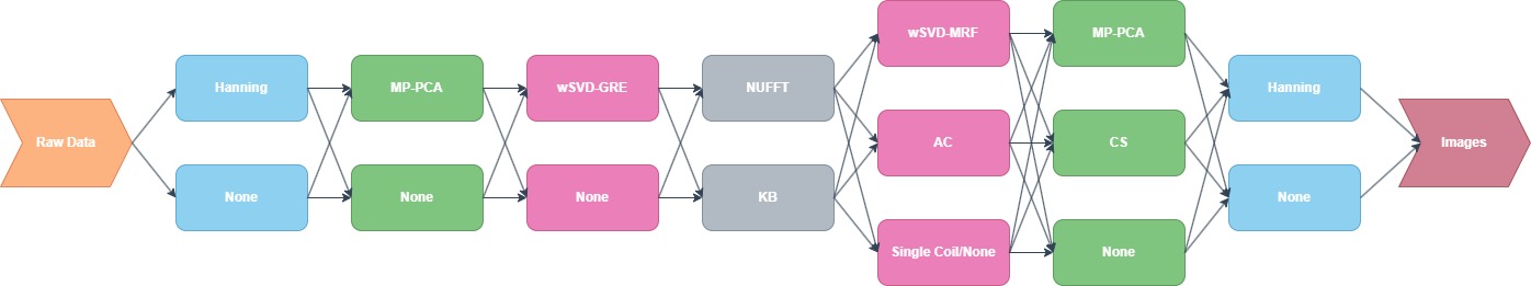
Figure 1: Flowchart of the toolbox DRAFT!

4.1 GRE Data

4.1.1 Phantom reconstruction and coil combination

In Figure 2, it can be seen that AC-KB clearly outperforms the other methods, which is also evident in Table 2 where the mean SNR in the region of interest is more than double that of wSVD-KB, the second-best method. One can also observe significantly lower SNR in the NUFFT reconstructions, which, however, still show a clear contrast against the background. Additionally, AC outperforms wSVD regardless of the reconstruction method. SoS performs poorly as it has both a low SNR and loses the structure of the water phantom with dropout at the edges.

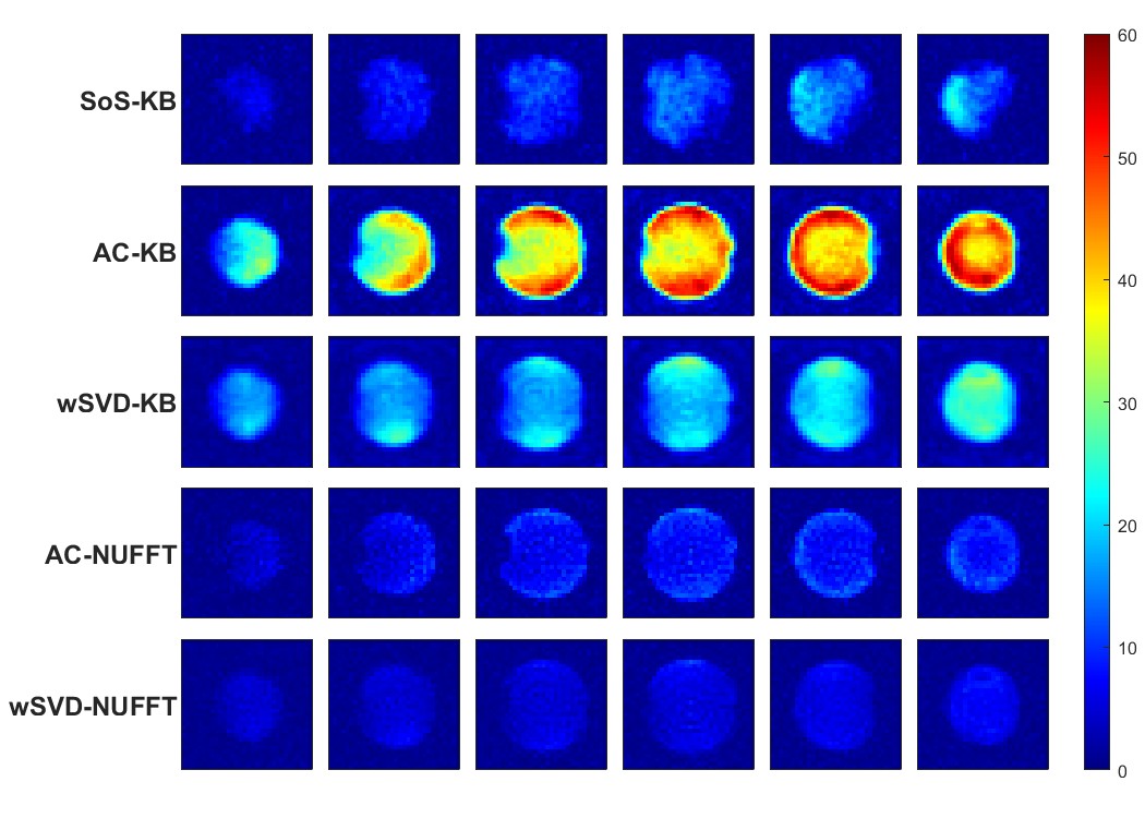
Figure 2: SNR plots of 6 axial slices of a water phantom, reconstructed using either KB-regridding or NUFFT, with coil combinations performed using SoS, AC, or wSVD.

4.1.2 Phantom denoising

The denoising performed on the 4x undersampled data reconstructed with KB and coils combined with AC can be seen in Figure 3. CS gives the highest SNR, close to the Non-Denoised reference, with values of 35.2 compared to 38.9 as seen in table 2. However, CS smoothes the images, which MP does not do. MP also significantly increases the SNR from the undersampled data.

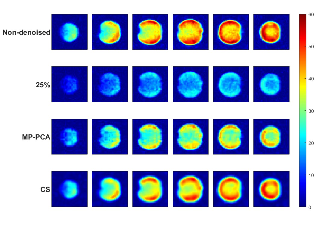
Figure 3: SNR plots of 6 axial slices of a water phantom reconstructed with KB-regridding and coils combined with AC. The plots are presented in the following order from top to bottom: the Non-denoised dataset, 4x downsampled before reconstruction, MP-PCA applied on the downsampled reconstruction, and CS applied on the downsampled reconstruction.

4.1.3 Invivo reconstruction and coil combination

Looking at the reconstructions from the full k-space data in Figure 4, one can observe a significant decrease in SNR compared to the phantom experiments. AC-KB performs the best, followed by wSVD-KB. The other methods fail to preserve the subject, making the brain invisible. While wSVD-KB provides some signal, it does not retain the structural details seen with AC-KB. This difference is also evident in Table 2, where the in vivo results are an order of magnitude lower than the phantom results, with means that are similar to their standard deviations.

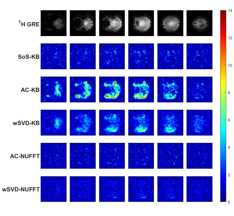
Figure 4: SNR plots of 6 axial slices of an invivo GRE scan for 100% of the k-space data, reconstructed using either KB-regridding or NUFFT, with coil combinations performed using SoS, AC, or wSVD.

4.1.4 Invivo denoising

For the denoising of in vivo data, the reconstructions with AC-KB using 100%, 66%, and 33% of the k-space are presented. One observes an increase in SNR for the full scan as the proportion of k-space data decreases, demonstrating the effectiveness of filtering. Referring to Table 2 and figure 5, it can also be seen that CS provides a larger SNR boost than MP-PCA. Both methods improve SNR compared to the non-denoised scan, but the effect diminishes as the k-space data is further filtered.

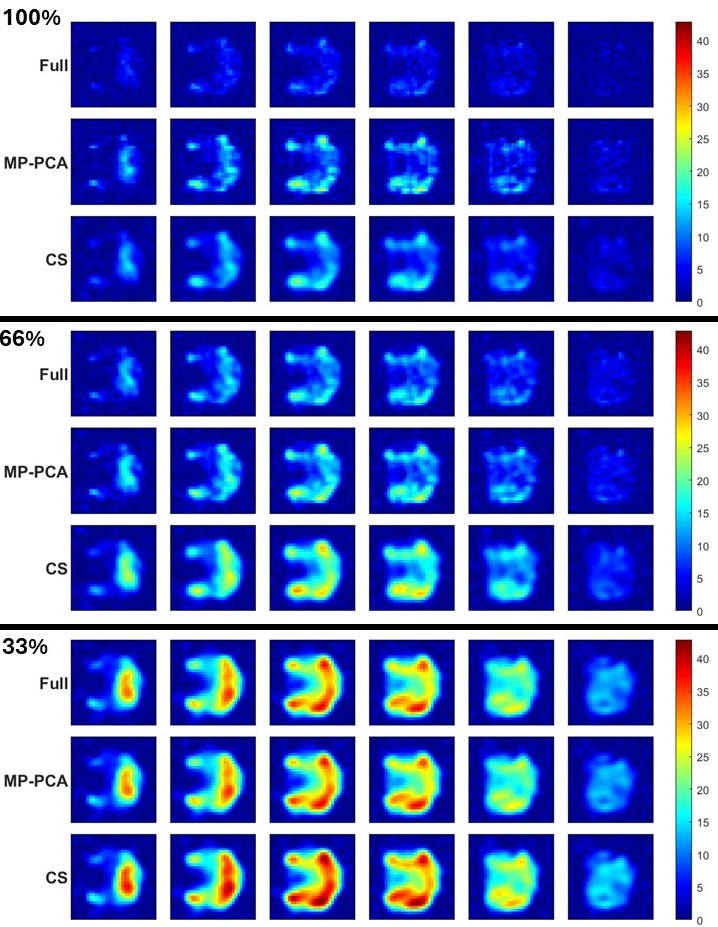
Figure 5: SNR plots of 6 axial slices of an in-vivo GRE phosphor scan reconstructed with KB-regridding and coils combined with AC.The plots are presented in the following order from top to bottom: For 100%, 66%, and 33% of the k-space being used, the Non-denoised dataset, MP-PCA applied on the Non-denoised dataset, and CS applied on the Non-denoised dataset.

4.2 GRE-table of results

Method	Mean	Std
Phantom reconstruction and coil combination
SoS-KB	9.5501	4.7057
AC-KB	37.8683	11.4736
wSVD-KB	17.0295	5.7184
AC-NUFFT	7.5008	3.0568
wSVD-NUFFT	4.7155	1.7972
Phantom denoising
Non-Denoised	38.1699	11.5591
Downsampled 4x	16.1521	5.3417
MP-PCA	28.8061	9.4193
CS	35.7023	10.2541
In vivo reconstruction and coil combination
SoS-KB	1.1366	0.89545
AC-KB	3.4351	2.4847
wSVD-KB	2.4332	1.2548
AC-NUFFT	0.91998	0.74126
wSVD-NUFFT	1.0475	0.56737
Invivo denoising
Non-Denoised 100%	3.4351	2.4847
CS 100%	7.8721	4.9691
MP-PCA 100%	7.1128	4.981
Non-Denoised 66%	8.0787	4.9134
CS 66%	15.0416	8.1952
MP-PCA 66%	10.4641	6.3464
Non-Denoised 33%	21.7342	10.3304
CS 33%	27.0285	12.827
MP-PCA 33%	21.7431	9.0882

Table 2: Mean and standard deviation of the SNR in the phantom and in vivo GRE SNR maps from high signal regions in three middle slices, as shown in Figures 10 and 11 where the top performer in every category is boldfaced

4.3 MRF Data

4.3.1 Reconstruction and coil combination

For the MRF results, similar patterns in both Figure 6 and Figure 7 are observed. While NUFFT performs weakly, it still exhibits contrast against the background. SoS produces images that appear as filtered noise. In terms of coil combination, wSVD provides the best images, both in terms of SNR and shape. AC, on the other hand, seems to weight the images downward, resulting in lopsided scans. These visual results are corroborated by the table of mean SNR (Table 3), where KB shows 3-4 times higher mean SNR, and wSVD has a higher SNR than AC when using KB as the reconstruction method.

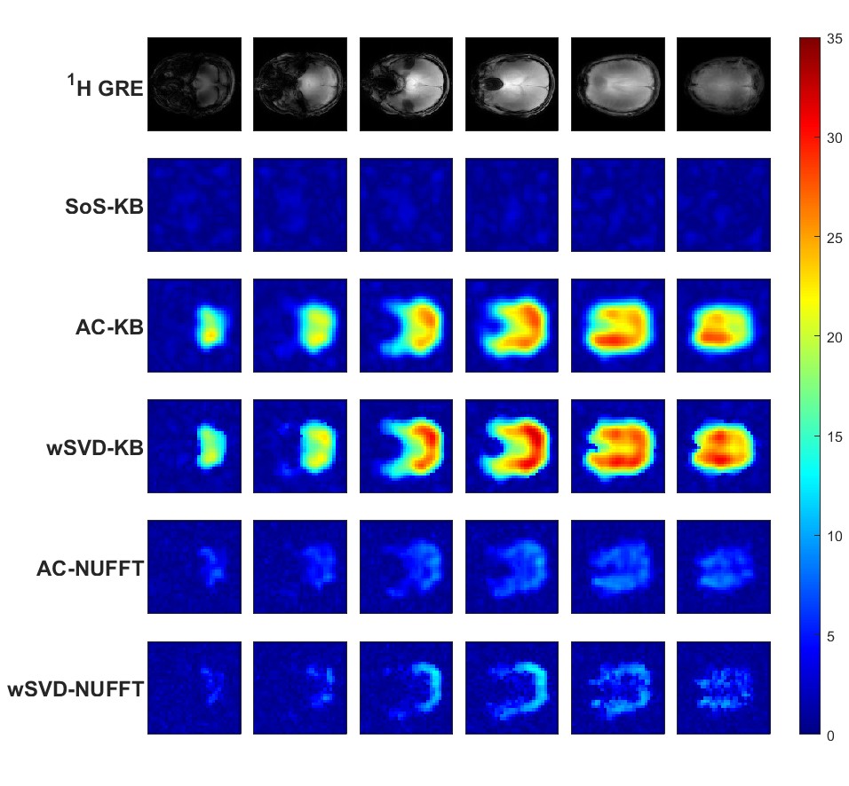
Figure 6: SNR plots of 6 axial slices of the ATP signal summed over 400 FAs, reconstructed using either KB-regridding or NUFFT, with coil combinations performed using SoS, AC, or wSVD.

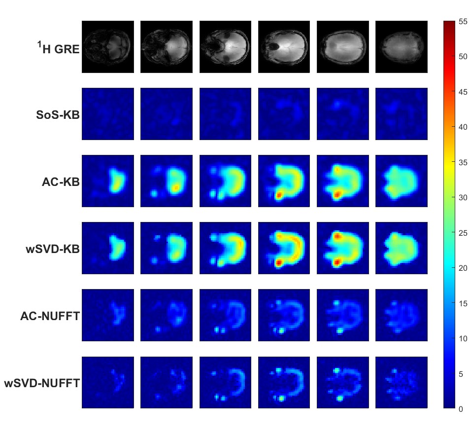
Figure 7: SNR plots of 6 axial slices of the PCr signal summed over 200 FAs, reconstructed using either KB-regridding or NUFFT, with coil combinations performed using SoS, AC, or wSVD.

4.3.2 Denoising

For the denoising results, ATP and PCr are examined separately, where the image rows are labeled as ”Denoising-method used on data” and ”Denoising-method used on images.” In Figure 8 and Table 3, it can be observed that denoising increases the SNR. However, applying denoising to the data changes the shape of the final ATP image. MP-PCA applied to the images introduces artifacts, particularly visible in the middle slices, while providing the highest SNR increase. CS results in a slight SNR increase if MP-PCA was not used on the data, but a more significant increase if it was. Applying MP-PCA to the data before reconstruction also boosts SNR but alters the image structure.

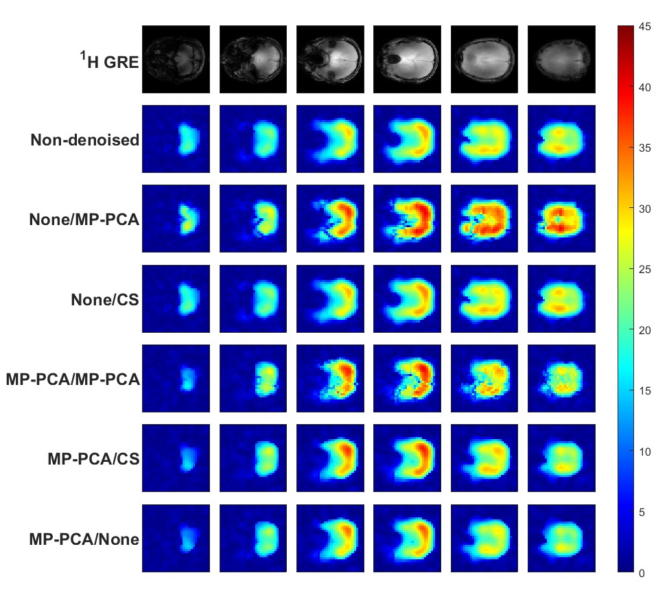
Figure 8: SNR plots of 6 axial slices of an ATP scan that was reconstructed with KB and coils combined with wSVD (Non-denoised). The titles for the rows are Denoising-method on data/Denoising-method on images.

In the denoising results for PCr shown in Figure 9, similar patterns to those seen with ATP can be observed. MP-PCA applied to the images introduces artifacts, while MP-PCA used on the data increases SNR without visibly altering the image structure. CS provides a consistent increase in SNR without introducing any visible defects in the images.

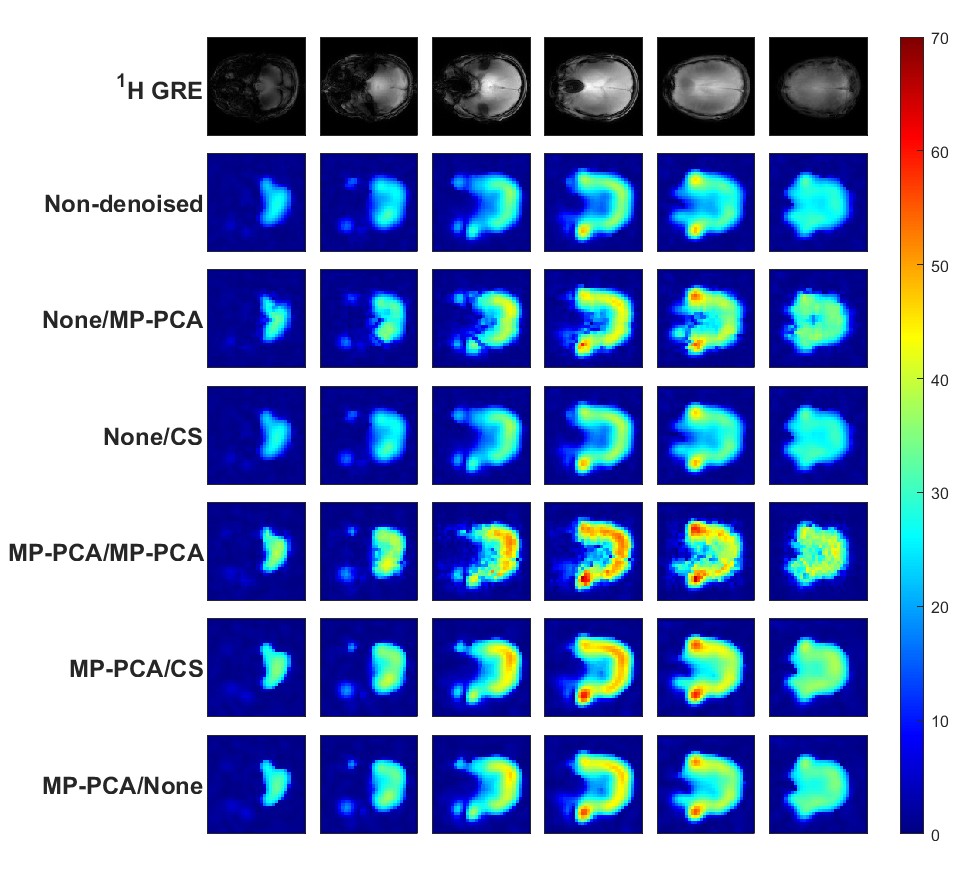
Figure 9: SNR plots of 6 axial slices of an PCr scan that was reconstructed with KB and coils combined with wSVD (Non-denoised). The titles for the rows are Denoising-method on data/Denoising-method on images.

4.4 Table of results

Method	Mean	Std
ATP reconstruction and coil combination
SoS-KB	0.82424	0.63283
AC-KB	16.2532	8.063
wSVD-KB	18.2012	8.811
AC-NUFFT	4.5669	2.5163
wSVD-NUFFT	4.2062	2.984
ATP denoising
Full	18.2012	8.811
MP-PCA/None	21.435	11.5
CS/None	18.7907	9.1647
MP-PCA/MP-PCA	17.1202	10.2054
MP-PCA/CS	17.3038	9.6832
MP-PCA/None	16.2934	8.9291
PCr reconstruction and coil combination
SoS-KB	1.9375	1.7273
AC-KB	20.5578	9.0612
wSVD-KB	22.2825	10.2448
AC-NUFFT	6.8712	3.9809
wSVD-NUFFT	5.4355	4.6627
PCR denoising
Full	22.2825	10.2448
MP-PCA/None	25.5486	12.7098
CS/None	23.9467	10.6135
MP-PCA/MP-PCA	28.6348	14.8116
MP-PCA/CS	28.0962	13.876
MP-PCA/None	26.0615	12.7786

Table 3: Mean and standard deviation of the SNR in the phantom and in vivo GRE SNR maps from high signal regions in three middle slices, as shown in Figures 12 and 13 where the top performer in every category is boldfaced

5 Discussion

5.1 GRE-results

The results seen in figures 2 and 4 clearly demonstrates the superior performance of the more advanced coil combination methods AC and wSVD which is further corroborated by table2. AC is also consequently better in the GRE-scans regardless of which method for reconstruction is used. In the phantom case we see a clear SNR boost while denoising where CS used on a 4x down-sampled dataset comes close to the full scan and MP-PCA also giving a clear SNR boost while not smoothing the image as CS does. In the invivo experiments in figure 5 we saw that MP-PCA and CS exhibit similar results to the phantom case where CS gives a larger SNR boost but smoothes the image while MP-PCA retains structure. Furthermore we saw that filtering the noisy data gives a remarkable SNR boost while reducing the efficacy of the denoising methods as they gave more than a 100% boost to the non-denoised images in the 100%-k-space experiments. These results are unexpected and contrary to the studies done on hydrogen data where NUFFT outperforms KB[20, 19]. This was investigated in the supplementary files where we see that NUFFT outperforms KB in a low noise environment where KB mostly smoothes, but if the noise power becomes too high NUFFT can no longer reliably reconstruct the data while KB still functions well. The behavior of CS is also clear, as it is very successful in artifact removal for NUFFT but less effective for denoising in high-noise environments. It also has a tendency to smooth results, influenced by the regularization parameter.

5.2 MRF-results

From the results in figures 6 and 7 KB gives the best results considering SNR with a large margin but NUFFT still preserves contrast. The best method is thus dependant on what the user searches for. However in contrast to the GRE experiments the amount of FAs makes time a relevant factor for MRF. NUFFT has a 10 times longer reconstruction time than KB of 0.4s and 0.04s respectively. Which then for 800 FAs makes a significant difference. Regarding the coil combination wSVD outperforms AC as it does not have downward gradient of signal as AC does. These results are consistent for both ATP and PCr but when denoising is applied they diverge from each other. The similarity of the methods are that when MP-PCA is applied on the images it creates artifacts while giving a SNR boost at the same time. The difference between the two is that MP-PCA applied on the data changes the structure of the shown ATP signal while it preserves PCr while boosting the SNR for both of them. This is believed to be from spikes in the ATP recordings which MP-PCA then mistakes for low frequency signals. CS gives a consistent SNR boost for both ATP and PCr and does not show any smoothing as in the GRE case.

6 Conclusions

We have demonstrated the capabilities of the SuperDuper31P toolbox demonstrating how different methods of reconstruction, coil combination and denoising performs on GRE and MRF type data. It was shown that Kaiser-Bessel regridding outperforms NUFFT in vivo if the noise power is high but vice-versa if low. Adaptive coil combination consistently outperformed wSVD in GRE data but the reverse was true in MRF. MP-PCA was great for GRE data and CS oversmoothed the image, in MRF MP-PCA ruined the images and CS gave a consistent boost without smoothing. Furthermore for a stack of spiral acquisition of 31-P GRE and MRF data we recommend using Filtering + AC-KB + MP-PCA and MP-PCA + wSVD-KB + CS respectively. Concluding, we saw that which method to use is highly dependant on type of acquisition/data and sensitive to hyper-parameters and possible artifacts in the data. Which motivates our investigation, and end result of a road map to utilize when deciding on methods to use in X-nuclei imaging, as the best performing ones differ from the analog hydrogen cases.

7 References

8 Supplementary files

8.1 Noise Calculation and max

Figure 10: Signal intensity map of the in phantom scan. The red rectangles indicate the locations used to calculate the noise standard deviation in the SNR maps. The pink squares represent the regions from which the SNR maximum and standard deviation were calculated in the region of interest.

Figure 11: Signal intensity map of the in vivo GRE scan. The red rectangles indicate the locations used to calculate the noise standard deviation in the SNR maps. The pink squares represent the regions from which the SNR maximum and standard deviation were calculated in the region of interest.

Figure 12: Signal intensity map of the in vivo ATP scan. The red rectangles indicate the locations used to calculate the noise standard deviation in the SNR maps. The pink squares represent the regions from which the SNR maximum and standard deviation were calculated in the region of interest.

Figure 13: Signal intensity map of the in vivo PCr scan. The red rectangles indicate the locations used to calculate the noise standard deviation in the SNR maps. The pink squares represent the regions from which the SNR maximum and standard deviation were calculated in the region of interest.

8.2 Invivo GRE coil combination for different percentages of k-space

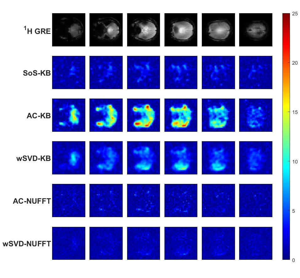
Figure 14: SNR plots of 6 axial slices of a in-vivo GRE phosphor scan using 66% of the k-space reconstructed with KB-regridding or NUFFT and coils combined with SoS, AC or wSVD

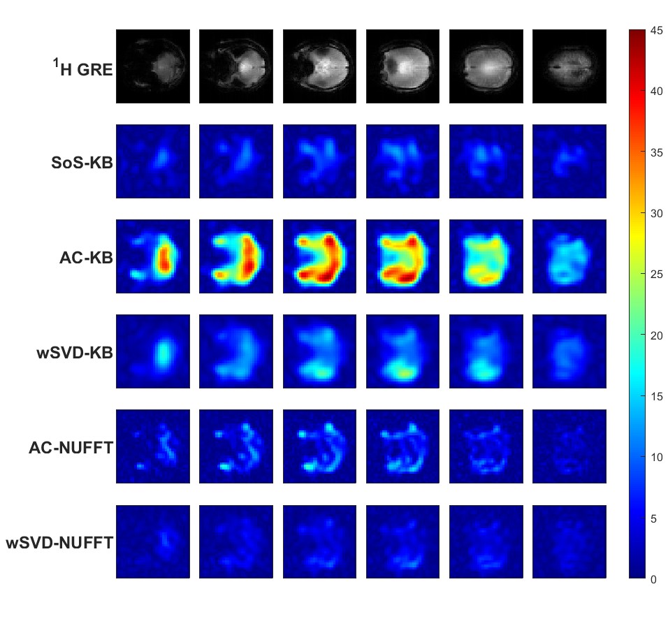
Figure 15: SNR plots of 6 axial slices of a in-vivo GRE phosphor scan using 33% of the k-space reconstructed with KB-regridding or NUFFT and coils combined with SoS, AC or wSVD

9 Compress sensing experiments

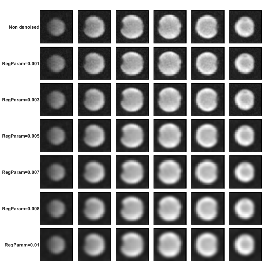
Figure 16: Six middle slices of a water phantom reconstructed with KB-AC and CS applied with a regularization parameter from 0.001 to 0.01

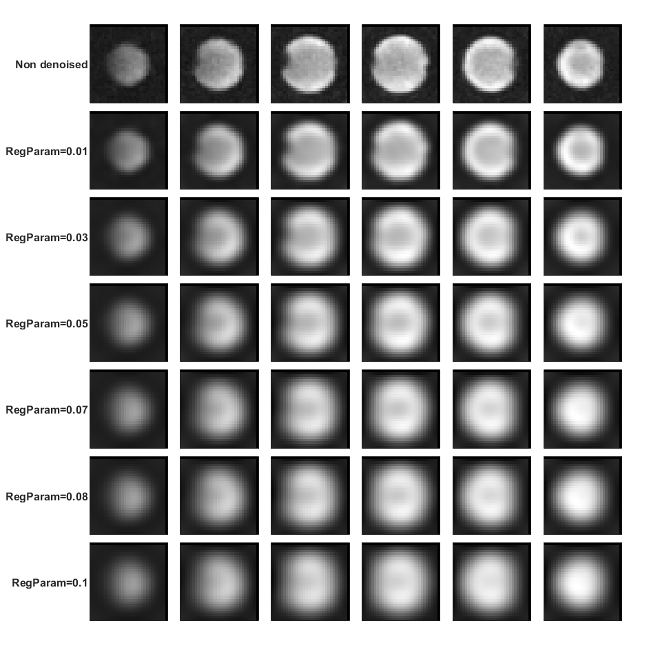
Figure 17: Six middle slices of a water phantom reconstructed with KB-AC and CS applied with a regularization parameter from 0.01 to 0.1

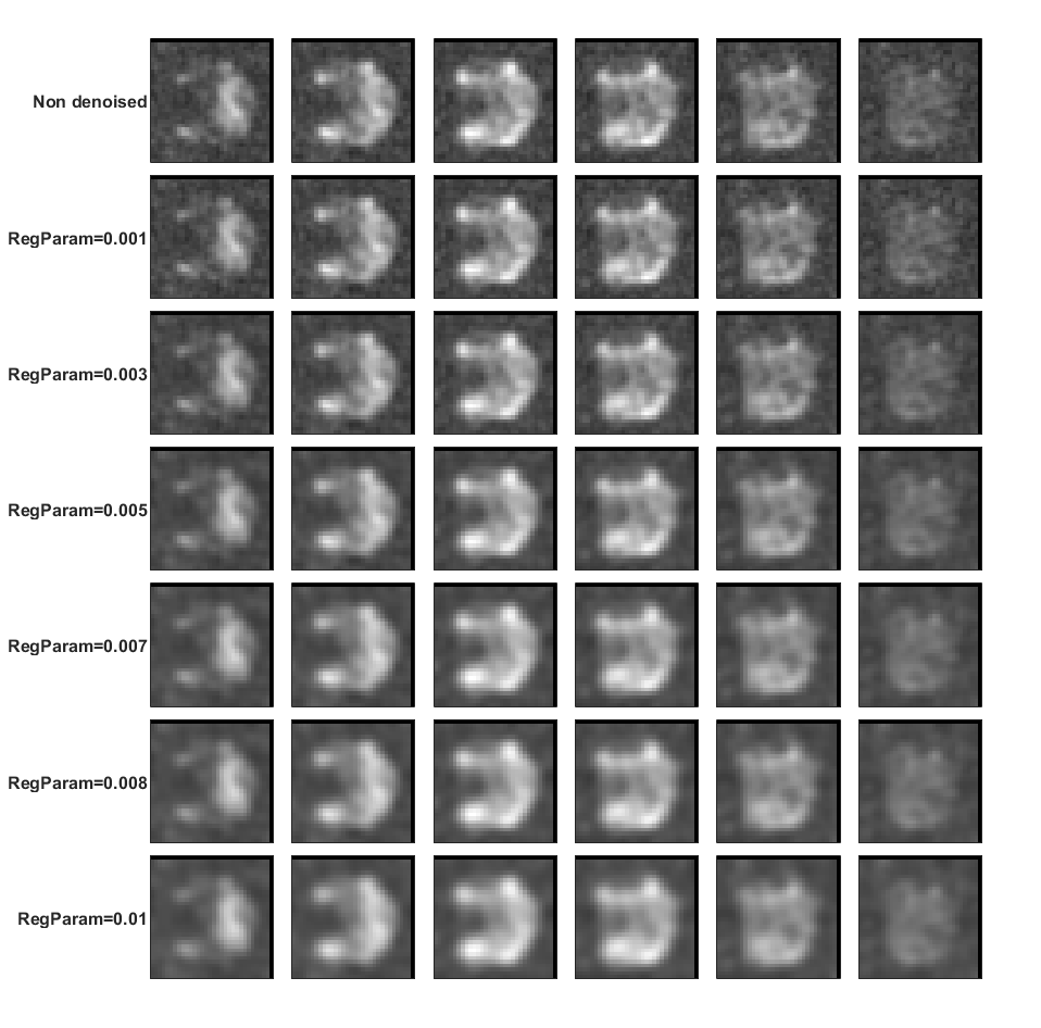
Figure 18: Six middle slices of a in vivo phosphor scan reconstructed with KB-AC using 66% of the k-space and CS applied with a regularization parameter from 0.001 to 0.01

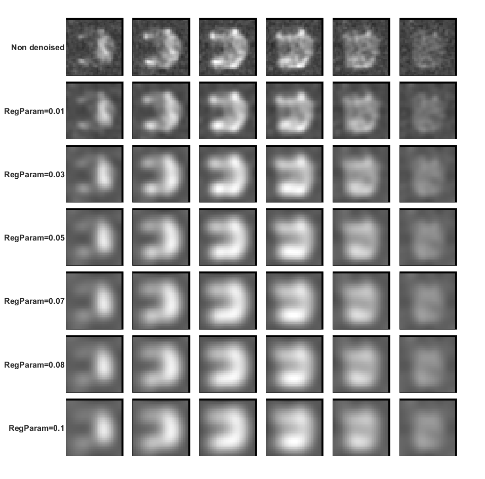
Figure 19: Six middle slices of a in vivo phosphor scan reconstructed with KB-AC using 66% of the k-space and CS applied with a regularization parameter from 0.01 to 0.1

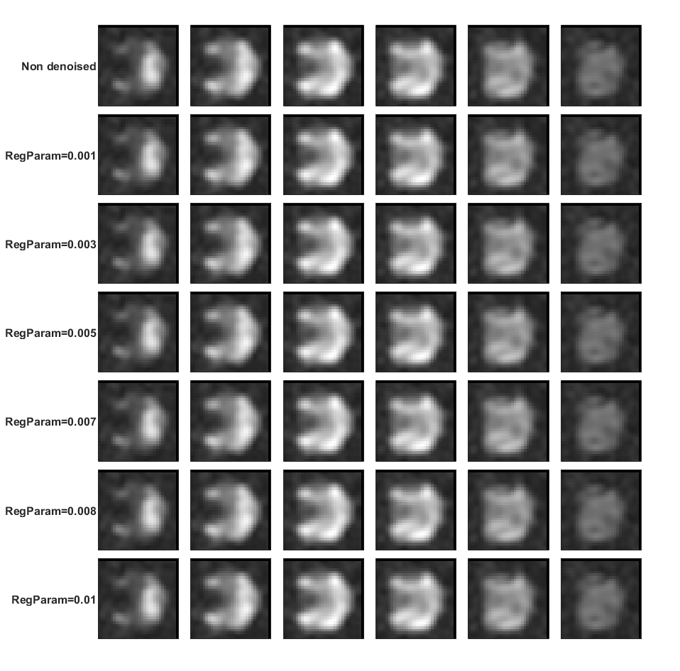
Figure 20: Six middle slices of a in vivo phosphor scan reconstructed with KB-AC using 33% of the k-space and CS applied with a regularization parameter from 0.001 to 0.01

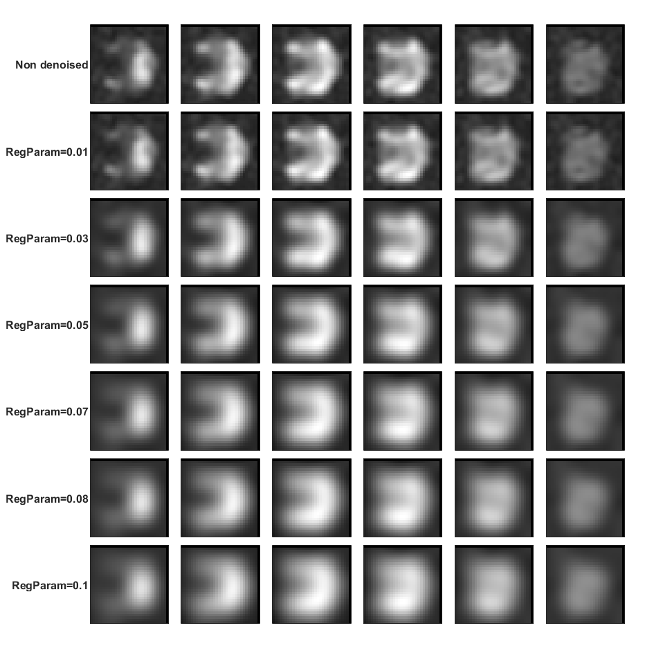
Figure 21: Six middle slices of a in vivo phosphor scan reconstructed with KB-AC using 33% of the k-space and CS applied with a regularization parameter from 0.01 to 0.1

10 Hydrogen results

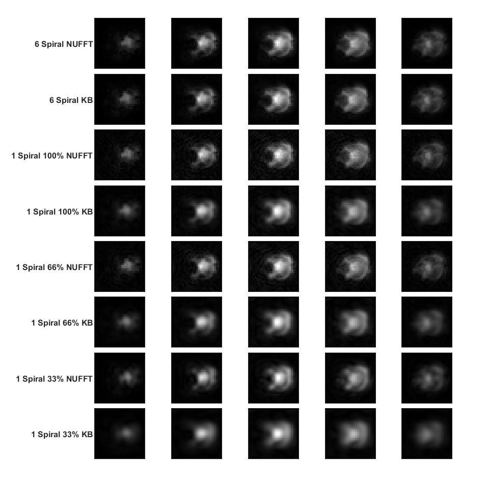
Figure 22: Hydrogen data reconstructed with NUFFT or KB using 6 spirals per slice or 1 while also decreasing the k-space sampling from 100%, 66%, and 33%

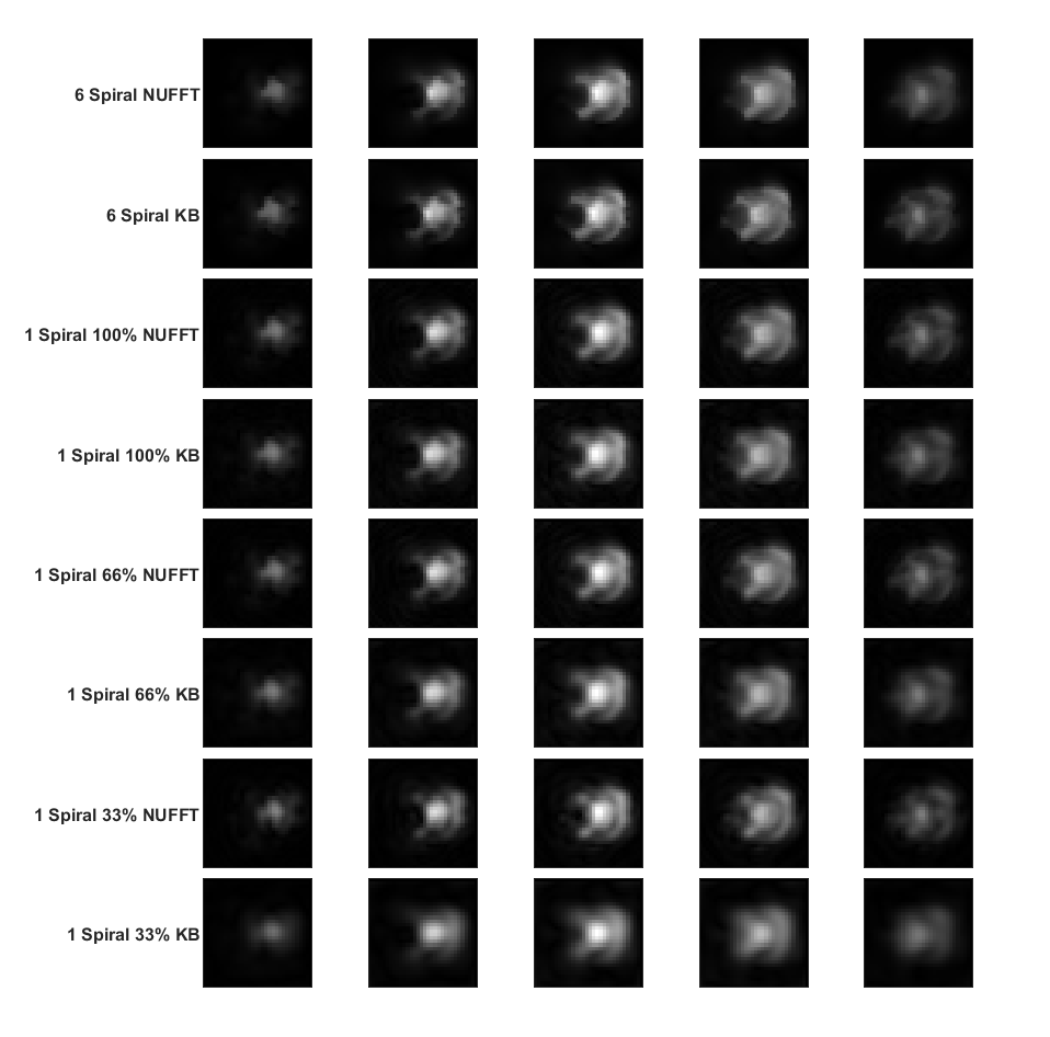
Figure 23: Hydrogen data reconstructed with NUFFT or KB using 6 spirals per slice or 1 while also decreasing the k-space sampling from 100%, 66%, and 33%, with CS applied with a 0.001 regularization parameter

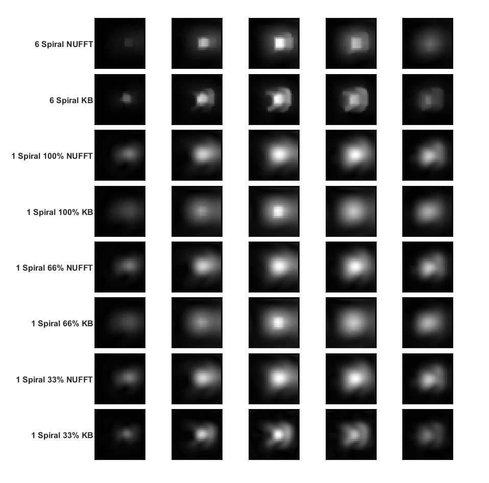
Figure 24: Hydrogen data reconstructed with NUFFT or KB using 6 spirals per slice or 1 while also decreasing the k-space sampling from 100%, 66%, and 33%, with CS applied with a 0.01 regularization parameter

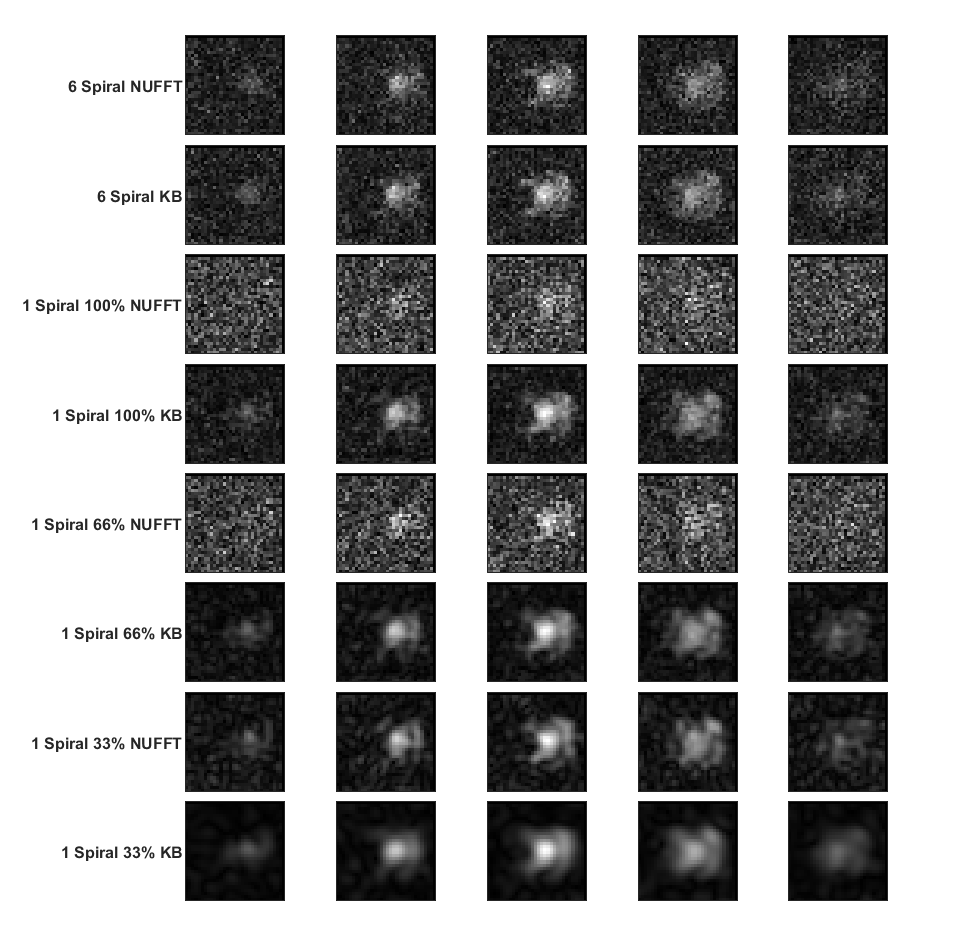
Figure 25: Hydrogen data reconstructed with NUFFT or KB using 6 spirals per slice or 1 while also decreasing the k-space sampling from 100%, 66%, and 33%, with added Gaussian noise

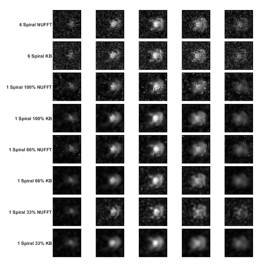
Figure 26: Hydrogen data reconstructed with NUFFT or KB using 6 spirals per slice or 1 while also decreasing the k-space sampling from 100%, 66%, and 33%, with added Gaussian noise and CS applied with a 0.001 regularization parameter

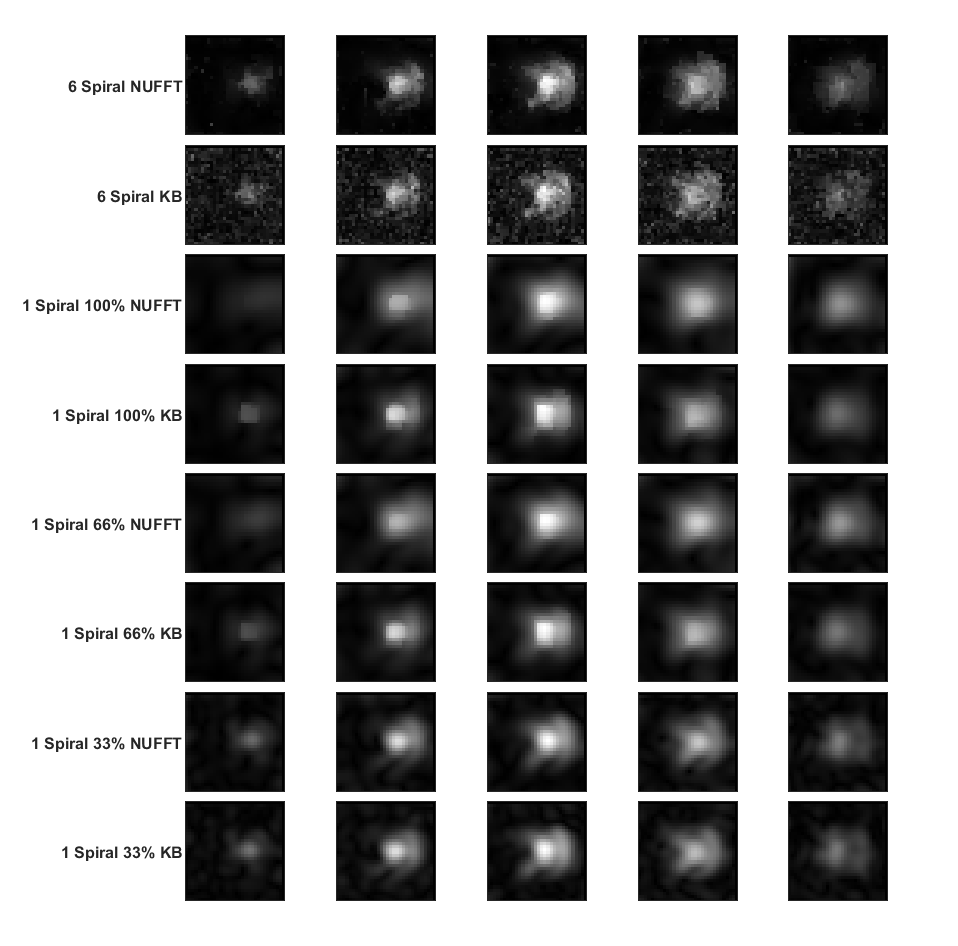
Figure 27: Hydrogen data reconstructed with NUFFT or KB using 6 spirals per slice or 1 while also decreasing the k-space sampling from 100%, 66%, and 33%, with added Gaussian noise and CS applied with a 0.003 regularization parameter

References

- [1] Chang-Hoon Choi, Suk-Min Hong, Jörg Felder and N. Shah “The state-of-the-art and emerging design approaches of double-tuned RF coils for X-nuclei, brain MR imaging and spectroscopy: A review” In Magnetic Resonance Imaging 72, 2020, pp. 103–116 DOI: https://doi.org/10.1016/j.mri.2020.07.003
- [2] D.. Klomp et al. “31P MRSI and 1H MRS at 7 T: initial results in human breast cancer” In NMR in Biomedicine 24.10, 2011, pp. 1337–1342 DOI: 10.1002/nbm.1696
- [3] R.. Deicken, G. Fein and M.. Weiner “Abnormal frontal lobe phosphorous metabolism in bipolar disorder” In The American Journal of Psychiatry 152.6, 1995, pp. 915–918 DOI: 10.1176/ajp.152.6.915
- [4] Mark E. Ladd et al. “Pros and cons of ultra-high-field MRI/MRS for human application” In Progress in Nuclear Magnetic Resonance Spectroscopy 109, 2018, pp. 1–50 DOI: https://doi.org/10.1016/j.pnmrs.2018.06.001
- [5] Mark Widmaier et al. “Fast 3D 31P B1+ mapping with a weighted stack of spiral trajectory at 7 Tesla”, 2024 arXiv: https://arxiv.org/abs/2406.18426
- [6] Ruomin Hu et al. “X-nuclei imaging: Current state, technical challenges, and future directions” In Journal of Magnetic Resonance Imaging 51.2, 2020, pp. 355–376 DOI: https://doi.org/10.1002/jmri.26780
- [7] Dan Ma et al. “Magnetic resonance fingerprinting” In Nature 495.7440, 2013, pp. 187–192 DOI: 10.1038/nature11971
- [8] Mark Widmaier, Song-I Lim, Daniel Wenz and Lijing Xin “Fast in vivo assay of creatine kinase activity in the human brain by 31P magnetic resonance fingerprinting” In NMR in Biomedicine 36.11, 2023, pp. e4998 DOI: https://doi.org/10.1002/nbm.4998
- [9] Charlie Yi Wang et al. “Magnetic resonance fingerprinting with quadratic RF phase for measurement of T2* simultaneously with f, T1, and T2” In Magnetic Resonance in Medicine 81.3, 2019, pp. 1849–1862 DOI: https://doi.org/10.1002/mrm.27543
- [10] Fabian J. Kratzer et al. “3D sodium (23Na) magnetic resonance fingerprinting for time-efficient relaxometric mapping” In Magnetic Resonance in Medicine 86.5, 2021, pp. 2412–2425 DOI: https://doi.org/10.1002/mrm.28873
- [11] Christopher T. Rodgers and Matthew D. Robson “Receive array magnetic resonance spectroscopy: Whitened singular value decomposition (WSVD) gives optimal Bayesian solution” In Magnetic Resonance in Medicine 63.4, 2010, pp. 881–891 DOI: https://doi.org/10.1002/mrm.22230
- [12] D.. Walsh, A.. Gmitro and M.. Marcellin “Adaptive reconstruction of phased array MR imagery” In Magnetic Resonance in Medicine 43.5, 2000, pp. 682–690 DOI: 10.1002/(sici)1522-2594(200005)43:5¡682::aid-mrm10¿3.0.co;2-g
- [13] Ken Sakaie and Mark Lowe “Retrospective correction of bias in diffusion tensor imaging arising from coil combination mode” In Magnetic Resonance Imaging 37, 2017, pp. 203–208 DOI: https://doi.org/10.1016/j.mri.2016.12.004
- [14] W. Hu et al. “Coil Combination of Multichannel Single Voxel Magnetic Resonance Spectroscopy with Repeatedly Sampled In Vivo Data” In Molecules 26.13, 2021, pp. 3896 DOI: 10.3390/molecules26133896
- [15] Christopher T. Rodgers and Matthew D. Robson “Coil combination for receive array spectroscopy: Are data-driven methods superior to methods using computed field maps?” In Magnetic Resonance in Medicine 75.2, 2016, pp. 473–487 DOI: 10.1002/mrm.25618
- [16] Vasiliki Mallikourti et al. “Optimal Phased-Array Signal Combination For Polyunsaturated Fatty Acids Measurement In Breast Cancer Using Multiple Quantum Coherence MR Spectroscopy At 3T OPEN” In Scientific Reports 9, 2019 DOI: 10.1038/s41598-019-45710-1
- [17] P.J. Beatty, D.G. Nishimura and J.M. Pauly “Rapid gridding reconstruction with a minimal oversampling ratio” In IEEE Transactions on Medical Imaging 24.6, 2005, pp. 799–808 DOI: 10.1109/TMI.2005.848376
- [18] J.A. Fessler and B.P. Sutton “Nonuniform fast Fourier transforms using min-max interpolation” In IEEE Transactions on Signal Processing 51.2, 2003, pp. 560–574 DOI: 10.1109/TSP.2002.807005
- [19] Jeffrey A. Fessler “On NUFFT-based gridding for non-Cartesian MRI” In Journal of Magnetic Resonance 188.2, 2007, pp. 191–195 DOI: 10.1016/j.jmr.2007.06.012
- [20] J. Song et al. “Least-square NUFFT methods applied to 2-D and 3-D radially encoded MR image reconstruction” In IEEE Transactions on Biomedical Engineering 56.4, 2009, pp. 1134–1142 DOI: 10.1109/TBME.2009.2012721
- [21] F. Riemer, B.S. Solanky and C. Stehning “Sodium (23Na) ultra-short echo time imaging in the human brain using a 3D-Cones trajectory” In Magnetic Resonance Materials in Physics, Biology and Medicine 27.1 Springer, 2014, pp. 35–46 DOI: 10.1007/s10334-013-0395-2
- [22] Guillaume Madelin, Jin-Suck Lee, Ravinder R. Regatte and Alexej Jerschow “Sodium MRI: methods and applications” In Progress in Nuclear Magnetic Resonance Spectroscopy 79 Elsevier, 2014, pp. 14–47 DOI: 10.1016/j.pnmrs.2014.02.001
- [23] Chandrasekhar Tippareddy, Wei Zhao and Jeffrey L. Sunshine “Magnetic resonance fingerprinting: an overview” In European Journal of Nuclear Medicine and Molecular Imaging 48 Springer, 2021, pp. 4189–4200 DOI: 10.1007/s00259-021-05384-2
- [24] Jean J.. Hsieh and Imants Svalbe “Magnetic resonance fingerprinting: from evolution to clinical applications” In Journal of Medical Radiation Sciences 67.4, 2020, pp. 333–344 DOI: https://doi.org/10.1002/jmrs.413
- [25] Amandeep Kaur and Guanfang Dong “A Complete Review on Image Denoising Techniques for Medical Images” In Neural Processing Letters 55.6, 2023, pp. 7807–7850 DOI: 10.1007/s11063-023-11286-1
- [26] Simon Koppers et al. “Sodium Image Denoising Based on a Convolutional Denoising Autoencoder” In Bildverarbeitung für die Medizin 2019 Wiesbaden: Springer Fachmedien Wiesbaden, 2019, pp. 98–103
- [27] Michael Lustig, David Donoho and John M. Pauly “Sparse MRI: The application of compressed sensing for rapid MR imaging” In Magnetic Resonance in Medicine 58.6, 2007, pp. 1182–1195 DOI: 10.1002/mrm.21391
- [28] Jong Chul Ye “Compressed sensing MRI: a review from signal processing perspective” In BMC Biomedical Engineering 1.1, 2019, pp. 8 DOI: 10.1186/s42490-019-0006-z
- [29] Florian Knoll, Kristian Bredies, Thomas Pock and Rudolf Stollberger “Second order total generalized variation (TGV) for MRI” In Magnetic Resonance in Medicine 65.2, 2011, pp. 480–491 DOI: https://doi.org/10.1002/mrm.22595
- [30] Qingping Chen, N. Shah and Wieland A. Worthoff “Compressed Sensing in Sodium Magnetic Resonance Imaging: Techniques, Applications, and Future Prospects” In Journal of Magnetic Resonance Imaging 55.5, 2022, pp. 1340–1356 DOI: https://doi.org/10.1002/jmri.28029
- [31] T. Speidel, P. Metze and V. Rasche “Efficient 3D Low-Discrepancy -Space Sampling Using Highly Adaptable Seiffert Spirals” In IEEE Transactions on Medical Imaging 38.8, 2019, pp. 1833–1840 DOI: 10.1109/TMI.2018.2888695
- [32] S. Moeller, S. Weingartner and M. Akcakaya “Multi-scale locally low-rank noise reduction for high-resolution dynamic quantitative cardiac MRI” In Annual International Conference of the IEEE Engineering in Medicine and Biology Society. IEEE Engineering in Medicine and Biology Society. Annual International Conference, 2017, pp. 1473–1476 DOI: 10.1109/EMBC.2017.8037113
- [33] Mark D. Does et al. “Evaluation of principal component analysis image denoising on multi-exponential MRI relaxometry” In Magnetic Resonance in Medicine 81.6, 2019, pp. 3503–3514 DOI: https://doi.org/10.1002/mrm.27658
- [34] Jelle Veraart, Els Fieremans and Dmitry S. Novikov “Diffusion MRI noise mapping using random matrix theory” In Magnetic Resonance in Medicine 76.5, 2016, pp. 1582–1593 DOI: 10.1002/mrm.26059
- [35] Jelle Veraart “Denoising of diffusion MRI using random matrix theory” In NeuroImage 142, 2016, pp. 394–406 DOI: 10.1016/j.neuroimage.2016.08.016