Search for continuous gravitational waves from unknown neutron stars in binary systems with long orbital periods in O3 data

Abstract

Gravitational waves emitted by asymmetric rotating neutron stars are the primary targets of continuous gravitational-wave searches. Neutron stars in binary systems are particularly interesting due to the potential for non-axisymmetric deformations induced by a companion star. However, all-sky searches for unknown neutron stars in binary systems are very computationally expensive and this limits their sensitivity and/or breadth. In this paper we present results of a search for signals with gravitational-wave frequencies between $50$ and $150$ Hz, from systems with orbital periods between $100$ and $1\,000$ days and projected semi-major axes between $40$ and $200$ light-seconds. This parameter-space region has never been directly searched before. We do not detect any signal, and our results exclude gravitational-wave amplitudes above $1.25\times 10^{-25}$ at $144.32$ Hz with $95\%$ confidence. Our improved search pipeline is more sensitive than any previous all-sky binary search by about $75\%$.

1 Introduction

Continuous gravitational waves from rotating neutron stars with a sustained quadrupole are one of the types of gravitational waves yet to be detected by ground-based detectors such as Advanced LIGO (for a recent review see Riles, 2023). The required quadrupole in the neutron star can be sourced by different mechanisms (see Jones & Riles, 2024), such as a mountain, characterized by the ellipticity of the neutron star (namely the difference between two moments of inertia not aligned with the rotational axis); r-modes, an oscillation mode of the star due to its rotation that can be unstable to gravitational-wave emission; Ekman-pumping (Singh, 2017, and references therein).

Continuous wave searches can be differentiated by the information we have about the emitting source: on one extreme there are targeted searches, where the source is a known pulsar; on the other extreme there are all-sky searches, where the source is completely unknown. Due to this lack of information, all-sky searches represent the most computationally demanding type of continuous wave search (Wette, 2023). These searches are interesting since most of the neutron stars in our galaxy have not yet been discovered.

Due to the large parameter space being investigated, all-sky searches usually employ semi-coherent methods, where the dataset is separated in smaller segments, which are analyzed coherently, and incoherently combined afterwards (see Tenorio et al. 2021 for a recent review). Although these methods are less sensitive than fully coherent ones, they reduce the required computational budget by a huge amount. After an initial search with a certain coherence time, any remaining candidates can be followed-up with a longer coherence time in a number of subsequent stages (Steltner et al., 2023; Abbott et al., 2022a; Dergachev & Papa, 2023).

When the unknown neutron star is in a binary system the search problem becomes even more challenging, since additional parameters need to be accounted for (Leaci & Prix, 2015). However, since more than half of the known millisecond pulsars are in binary systems (Manchester et al., 2005), and, additionally, accretion offers an additional mechanism to generate the quadrupole needed for a detectable continuous wave, searching for signals from unknown neutron stars in binaries is of utmost importance.

In this paper we present a search with two main novelties: (i) the parameter space region that we investigate has never been directly searched before; (ii) the sensitivity that our search attains is $75\%$ better than any previous search of this kind. We cover gravitational-wave frequencies between 50 and 150 Hz, orbital periods between 100 and $1\,000$ days, and projected semi-major axes between 40 and 200 light-seconds (see Figure 2).

This search uses the public O3 data from the Advanced LIGO detectors, and attains a sensitivity depth of $38.6$ $\textrm{Hz}^{-1/2}$. We use the most sensitive search pipeline available for this type of search, BinarySkyHou$\mathcal{F}$ (Covas & Prix, 2022a), which combines the coherent $\mathcal{F}$-statistic (Jaranowski et al., 1998) with the Hough transform method (Krishnan et al., 2004). Although we do not detect any signal, we are able to place upper limits on the gravitational-wave amplitude at a level of $1.25\times 10^{-25}$ at $144.32$ Hz with $95\%$ confidence. Furthermore, due to the low coherence time of the main search and of the follow-ups ($0.05$ days to $1.56$ days), this search is robust to unmodeled effects such as spin-wandering (Mukherjee et al., 2018), neutron star glitches (Ashton et al., 2017), or timing noise (Ashton et al., 2015), which may become important on the timescale of many days.

The paper is organized as follows: in Section 2 we introduce the signal model that we assume; in Section 3 we describe the data that we use, the parameter space that we cover, the pipeline that we use, and the search that was done; in Section 4 we present our results and discuss their astrophysical implications; in Section 5 we conclude the paper.

2 Signal model

We assume that the continuous wave signal $h(t)$ as a function of time $t$ in the detector frame is given by (Jaranowski et al., 1998):

$$h(t)=h_{0} \left[F_{+}(t;\psi)\frac{1+\cos^{2}{\iota}}{2}\cos{[\phi_{0}+\phi(t)]}\right.$$

$$+ \left.F_{\times}(t;\psi)\cos{\iota}\sin{[\phi_{0}+\phi(t)]}\right],$$ (1)

where $F_{+}$ and $F_{\times}$ are the antenna-pattern functions of the detector (given in Jaranowski et al., 1998), $\iota$ is in the angle between the angular momentum of the neutron star and the line of sight, $\psi$ is the polarization angle, $\phi_{0}$ is the initial phase, $\phi(t)$ is the gravitational-wave phase at time $t$, and $h_{0}$ is the intrinsic gravitational-wave amplitude.

The phase of the signal $\phi(t)$ in the detector frame depends on the intrinsic gravitational-wave frequency $f_{0}$ and frequency derivatives of the signal $f_{1},...,f_{k}$, and on the Doppler modulation due to the relative motion between the neutron star and the detector. This Doppler modulation depends on the sky position of the source (given by $\alpha$ and $\delta$) and on the orbit of the neutron star around the binary barycenter, described by the orbital period $P_{\mathrm{orb}}$, the projected semi-major axis $a_{\mathrm{p}}$, the time of ascension $t_{\mathrm{asc}}$, the argument of periapsis $\omega$, and the eccentricity $e$, as discussed by Leaci & Prix (2015). Here we search for sources with a small enough spin-down and eccentricity to not require that we search over these parameters in order to accurately track the signal in the first stage of the search, as reflected in Table 1.

3 The search

3.1 Data

This search uses O3 public data (LIGO, Virgo, KAGRA collaborations, 2021a, b) of the Advanced LIGO Hanford (H1) and Advanced LIGO Livingston (L1) gravitational-wave detectors (Aasi et al., 2015). The data-span covers from April 2019 to March 2020, with a month-long interruption for commissioning interventions. The average duty factor is $\sim 74\%$. We use the GWOSC-16KHZ_R1_STRAIN channel and the DCS-CALIB_STRAIN_CLEAN_SUB60HZ_C01_AR frame type.

A linear and non-linear noise subtraction procedure was applied to this data before public release at the harmonics of the mains 60 Hz lines and the calibration lines (Davis et al., 2019) in order to remove some of the non-Gaussian sinusoidal-like noise features present in the dataset (Covas et al., 2018). Many other lines still contaminate the dataset, which produce spurious outliers that need to be individually examined and discarded, as will be seen in Section 3.5.

This dataset also suffers from a large number of short-duration glitches that increase the noise level in the frequency range of interest for this search, thus reducing its sensitivity, as discussed in other publications (e.g. Abbott et al., 2022b). For this reason, we use the gating method developed by Steltner et al. (2022) to remove these glitches and improve data quality.

The dataset of each detector is divided in short Fourier transforms (SFTs, see Allen & Mendell, 2004) of 200 s, short enough so that the signal power does not spread by more than a frequency bin during this time. The total number of SFTs is $105\,111$ for H1 and $105\,269$ for L1. The harmonic mean amplitude spectral density $\sqrt{S_{n}}$ of the Advanced LIGO detectors in the frequency range covered by this search is shown in Figure 1.

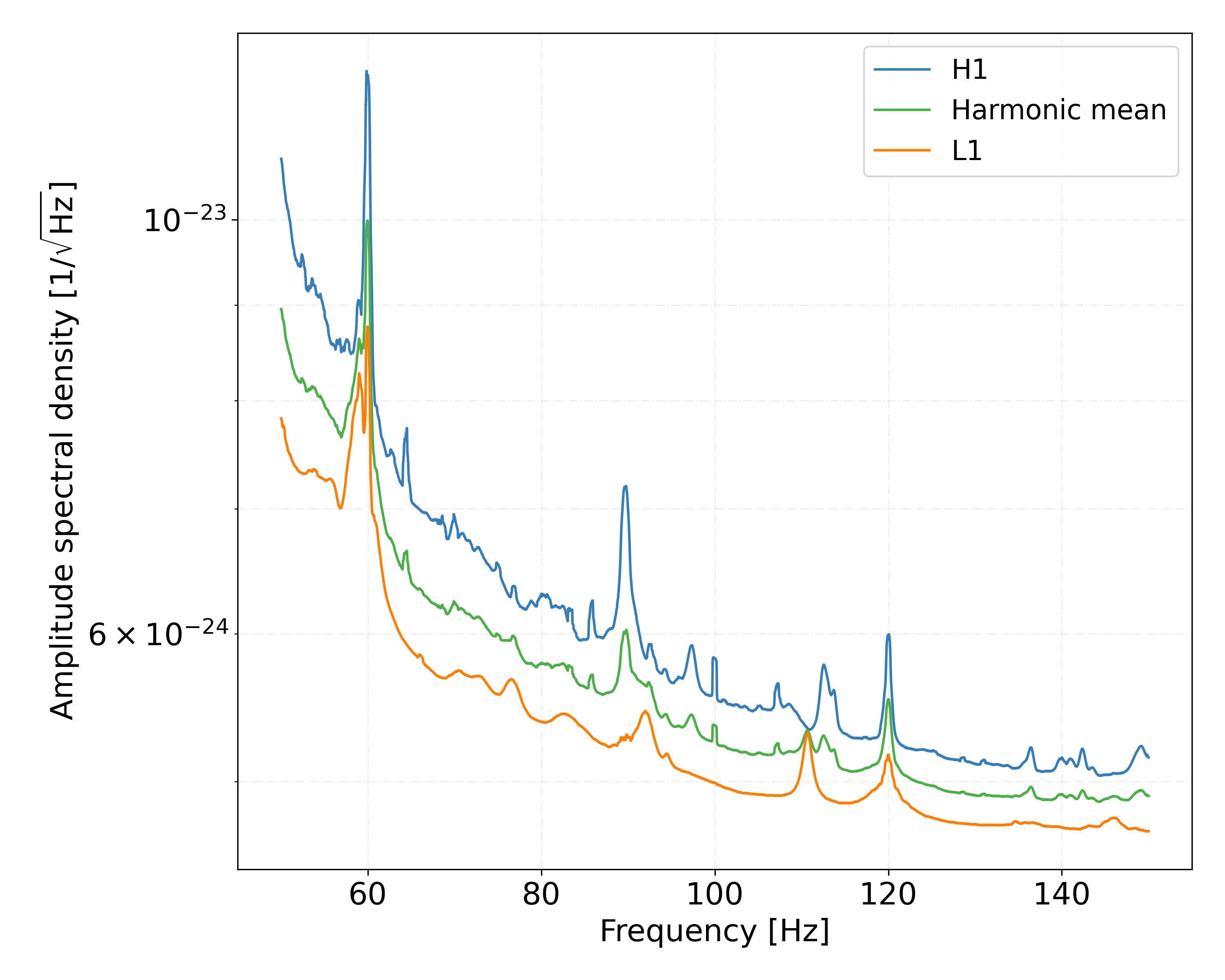
Figure 1: Harmonic mean (over $105\,111$ and $105\,269$ SFTs of 200 s for H1 and L1, respectively) of the amplitude spectral density $\sqrt{S_{n}}$ of the data used in this search as a function of frequency. The upper blue curve shows H1, the lower orange curve shows L1, and the middle green curve shows the harmonic mean between the two.

3.2 Parameter space covered

The signal parameter space covered by the search is summarized in Table 1. We search for signals across the entire sky with gravitational-wave frequencies $f_{0}$ between 50 and 150 Hz and frequency derivatives $|f_{1}|\leq 7.6\times 10^{-12}$ Hz/s. The frequency range is chosen as a balance between the sensitivity of the detectors (see Figure 1), the computational cost of the search (which grows $\propto f_{0}^{5}$), and the observed rotational frequencies of the pulsar population (5 out of 17 known pulsars in our $(P_{\mathrm{orb}},a_{\mathrm{p}})$ range fall in this frequency range), as shown in Figure 2. The chosen frequency derivative range allows us to set $f_{1}=0$ Hz/s for all templates in the first stage of the search while keeping the average mismatch below $\lesssim 0.3$. With the most rapidly varying rotation frequency of any millisecond pulsar in a binary system being $\sim 10^{-14}$ Hz/s (Manchester et al., 2005), our search range comfortably covers the observed range.

Neutron stars in binary systems display a broad range of projected semi-major axes $a_{\mathrm{p}}$, depending on the mass of the companion $M_{\mathrm{C}}$, on the inclination angle of the orbital plane $\iota_{\mathrm{b}}$, and on the orbital period $P_{\mathrm{orb}}$, as shown in Figure 2. All-sky searches with high sensitivity over such a broad range of parameters are currently impossible due to their prohibitive computational cost, so we limit the search to the range in $(P_{\mathrm{orb}},a_{\mathrm{p}})$ indicated by the red box in that Figure and given in Table 1. The parameter space contained in this box has not been directly searched in any previous search (Aasi et al., 2014; Covas & Sintes, 2020; Covas et al., 2022; Abbott et al., 2021, 2023a). The neutron stars targeted by this search have companions with masses on the order of a solar mass (mostly helium white dwarfs), and typically present smaller rotational frequencies than those inhabiting other regions of the $(P_{\mathrm{orb}},a_{\mathrm{p}})$ space.

Finally, in the first stage of the search we also set all templates to $e=0$ and do not explicitly search over eccentricity (and argument of periapsis).

Assuming small eccentricity, we estimate the maximum eccentricity covered by this search using Equations (15), (62), and (64) of Leaci & Prix (2015) with a metric mismatch of $\mu=1$:

$$e_{\mathrm{max}}=0.08\,\left({150\,\textrm{Hz}\over{f_{0}}}\right)\left({{P_{\mathrm{orb}}}\over 1\,000\,\textrm{days}}\right)\left({200\,\textrm{l-s}\over{a_{\mathrm{p}}}}\right).$$ (2)

For those ($f_{0},P_{\mathrm{orb}},a_{\mathrm{p}}$) that yield large $e_{\mathrm{max}}$ values, however, the assumptions of Equation 2 do not hold and can give rise to observed mismatches larger than expected. As a pragmatic fix, we cap Equation 2 at $e_{\mathrm{max}}\leq 0.1$.

Table 1: Range of values for the different parameters covered by the search. Only a single template is required by the first search to cover the ranges in first frequency derivative $f_{1}$, in eccentricity $e$, and in the argument of periapsis $\omega$. $t_{m}$ is the mid-time of the search, equal to $1\,253\,764\,659.5$ (GPS), which is used as the reference time.

Parameter	Range
$f_{0}$ [Hz]	[50, 150]
$|{f_{1}}|$ [Hz/s]	$<7.6\times 10^{-12}$
$\alpha$ [rad]	[0, $2\pi$)
$\delta$ [rad]	[$-\pi/2$, $\pi/2$]
$a_{\mathrm{p}}$ [l-s]	[40, 200]
$P_{\mathrm{orb}}$ [days]	[100, $1\,000$]
$t_{\mathrm{asc}}$ [GPS]	[$t_{m}-P_{\mathrm{orb}}/2$, $t_{m}+P_{\mathrm{orb}}/2$)
$e$	$<\min\left[0.1,e_{\max{}}\right]$ (see Equation (2))
$\omega$ [rad]	[0, $2\pi$)

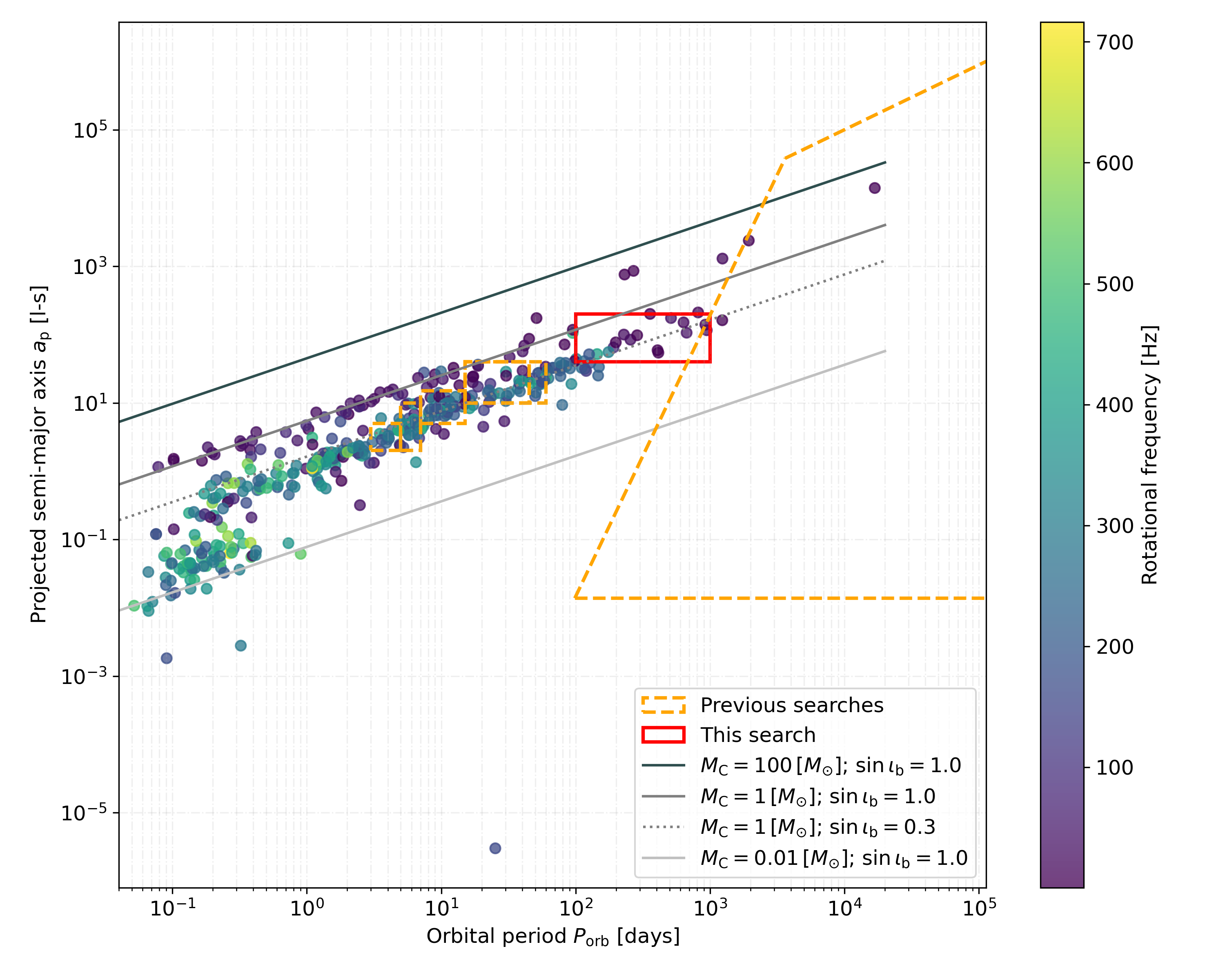
Figure 2: The red box shows the ranges in $(P_{\mathrm{orb}},a_{\mathrm{p}})$ covered by this search, while the points show the population of known pulsars in binary systems from the ATNF catalogue version 2.1.1 (Manchester et al., 2005). The orange dashed boxes show the ranges covered by previous searches using Advanced LIGO data (Covas & Sintes, 2020; Abbott et al., 2021; Covas et al., 2022). The orange box to the right is the region where the results of Singh & Papa (2023) apply, and partially overlaps with this search. The color scale shows the rotational frequency of each pulsar. The different gray lines show Kepler’s third law for different values of the companion mass $M_{\mathrm{C}}$ and inclination of the binary orbit $\iota_{\mathrm{b}}$, assuming a neutron star mass of 1.4 M_⊙.

3.3 Target signal population

Various parameters of the search, such as follow-up thresholds and veto parameters, are chosen to ensure safety (i.e. very low false dismissal probability) of the target signal population. The parameters of this target population are drawn from the search ranges given in Table 1, with uniform distributions on $\cos\iota$, $\psi$ and $\phi_{0}$ from Equation (2). All search parameters are sampled uniformly, except for sky position, which is drawn isotropically. The frequency $f_{0}$ is drawn uniformly in ten different 0.1 Hz bands ($56.3,59.3,63.2,77.5,83.1,85.5,100.1,101.5,131.3,148.2$). Spin-down $f_{1}$ and eccentricity $e$ are log-uniformly distributed with a lower limit two orders of magnitude below the maximum given in Table 1.

The amplitudes $h_{0}$ are chosen by uniformly sampling the sensitivity depth (see Equation (7)) from the range $[15,110]$ Hz^-1/2 (in discrete steps of $5$ Hz^-1/2). We use a total set of 50 000 signals, with 250 signals for each frequency and sensitivity depth. For the follow-up tests presented in Section 3.6, we use a subset of 2 000 signals (10 signals for each frequency and sensitivity depth) due to the high computational cost of these tests.

3.4 Stage 0

For the first stage of the search, which scans the entire parameter space, we use a semi-coherent search method where the data is separated in segments of a span $T_{\mathrm{coh}}=4\,500$ s, a value selected to balance computational cost constraints and sensitivity. We use BinarySkyHou$\mathcal{F}$ (Covas & Prix, 2022a), which currently is the most sensitive pipeline for these types of searches.

For each segment $\ell=1,\dots,N_{\mathrm{seg}}$ we calculate the coherent multi-detector dominant-response detection statistic $\mathcal{F}_{\mathrm{AB};\ell}$ (Covas & Prix, 2022b) over a coarse grid in $f$ and sky. Using $\mathcal{F}_{\mathrm{AB}}$ instead of the classic $\mathcal{F}$-statistic yields sensitivity gains for these short segments due to the reduced number of degrees of freedom.

This is the longest coherence time $T_{\mathrm{coh}}$ used so far in an all-sky search for neutron stars in binary systems, resulting in the most sensitive search. However, it is short enough so that the orbital parameters $(P_{\mathrm{orb}},a_{\mathrm{p}},t_{\mathrm{asc}})$ are not resolved at the coherent stage.

By combining the information from the different $\mathcal{F}_{\mathrm{AB};\ell}$ over the entire observation time, we can refine our ability to localize where a signal comes from in the sky, as well as the values of its orbital parameters. In practice this means that the grids used for the single-segment searches are not fine enough for combining together those results.

We set up a finer sky-grid and grids in $\lambda^{\mathrm{orb}}\equiv(P_{\mathrm{orb}},a_{\mathrm{p}},t_{\mathrm{asc}})$, and compute the detection statistic at each point by adding together appropriately the results computed in the coarse-grid template. The Hough master equation specifies what “appropriately” means as it determines at every segment which is the closest coarse template $\lambda^{\mathrm{coarse}}_{\ell}=(f^{\textrm{coarse}}_{\ell},{\textrm{sky}}^{\textrm{coarse}}_{\ell})$ to the template ($f_{0},\lambda^{\mathrm{orb}},\textrm{sky}$) for which we wish to compute the detection statistic (Covas & Prix, 2022a):

$$\hat{\mathcal{F}}_{\mathrm{ABw}}(f_{0},\lambda^{\mathrm{orb}},\textrm{sky})\equiv\sum_{\ell=1}^{N_{\mathrm{seg}}}w_{\ell}\,\mathcal{F}_{\mathrm{AB};\ell}(\lambda^{\mathrm{coarse}}_{\ell}),$$ (3)

where $N_{\mathrm{seg}}=5\,910$ and

$$w_{\ell}\propto\begin{cases}\frac{A_{\ell}+\frac{C_{\ell}^{2}}{A_{\ell}}}{S_{\mathrm{n;}\ell}}&\text{if }A_{\ell}\geq B_{\ell},\\ \frac{B_{\ell}+\frac{C_{\ell}^{2}}{B_{\ell}}}{S_{\mathrm{n;}\ell}}&\text{otherwise}.\end{cases}$$ (4)

$A$, $B$, and $C$ are the antenna-pattern matrix coefficients (Jaranowski et al., 1998) calculated at each coarse sky point. The weights are normalized as $\sum_{\ell}w_{\ell}=N_{\mathrm{seg}}$.

For each coarse sky-grid point we do not compute $\mathcal{F}_{\mathrm{AB};\ell}$ for segments with $w_{\ell}$ values in the 25th percentile and lower (Covas & Prix, 2022a; Behnke et al., 2015). This reduces the computational cost of the search while incurring a loss of sensitivity smaller than $\sim 5\%$. All segments are however used to recalculate the detection statistic for the top $1\%$ templates of each frequency band.

We define a significance $s$ (also called critical ratio) for every template as

$$s=\frac{\hat{\mathcal{F}}_{\mathrm{ABw}}-\mu_{\mathcal{F}}}{\sigma_{\mathcal{F}}},$$ (5)

where $\mu_{\mathcal{F}}$ is the expected mean and $\sigma_{\mathcal{F}}$ is the standard deviation of $\hat{\mathcal{F}}_{\mathrm{ABw}}$ in Gaussian noise, given by:

$$\mu_{\mathcal{F}}=2N_{\mathrm{seg}},\quad\sigma_{\mathcal{F}}^{2}=4\sum\limits_{\ell=1}^{N_{\mathrm{seg}}}w^{2}_{\ell}.$$ (6)

The search is divided in frequency bands of 0.1 Hz. The total number of templates searched is $\sim 1.05\times 10^{16}$, which are shown for each of the 0.1 Hz bands in Figure 3. The grid resolutions for all the parameters are shown in Table 2. These resolutions are obtained by using Equations 30-32 of Covas & Sintes (2019) with metric mismatch $\mu=1$ in each dimension; Equation 34 with $P_{\mathrm{F}}=0.8$; and half of the value given in Equation 33 for $f_{0}$. The overall resulting average mismatch produced by our template grid is $\lesssim 0.3$ and the mismatch distributions at two different frequencies are shown in Figure 4. We use finer coherent and semi-coherent grids for this search in order to increase its sensitivity compared to previous searches of this kind such as Covas et al. (2022).

Table 2: Grid resolutions for the different parameters in the first stage of the search. $\Omega=2\pi/P_{\mathrm{orb}}$ is the average angular orbital velocity.

Parameter	Resolution
$\delta f_{0}$ [Hz]	$1.1\times 10^{-4}$
$\delta\alpha$ [rad]	$1.9\times 10^{-2}\,\left({{150\,\tiny{\textrm{Hz}}}\over{f_{0}}}\right)$
$\delta\delta$ [rad]	$1.9\times 10^{-2}\,\left({{150\,\tiny{\textrm{Hz}}}\over{f_{0}}}\right)$
$\delta a_{\mathrm{p}}$ [l-s]	$3.2\times 10^{1}\,\left({{150\,\tiny{\textrm{Hz}}}\over{f_{0}}}\right)\left({{P_{\mathrm{orb}}\over{1\,000\,\tiny{\textrm{days}}}}}\right)$
$\delta\Omega$ [Hz]	$1.8\times 10^{-8}\,\left({{150\,\tiny{\textrm{Hz}}}\over{f_{0}}}\right)\left({{P_{\mathrm{orb}}\over{1\,000\,\tiny{\textrm{days}}}}}\right)\left({{200\,\tiny{\textrm{l-s}}}\over{a_{\mathrm{p}}}}\right)$
$\delta t_{\mathrm{asc}}$ [GPS]	$2.2\times 10^{6}\,\left({{150\,\tiny{\textrm{Hz}}}\over{f_{0}}}\right)\left({{P_{\mathrm{orb}}\over{1\,000\,\tiny{\textrm{days}}}}}\right)^{2}\left({{200\,\tiny{\textrm{l-s}}}\over{a_{\mathrm{p}}}}\right)$

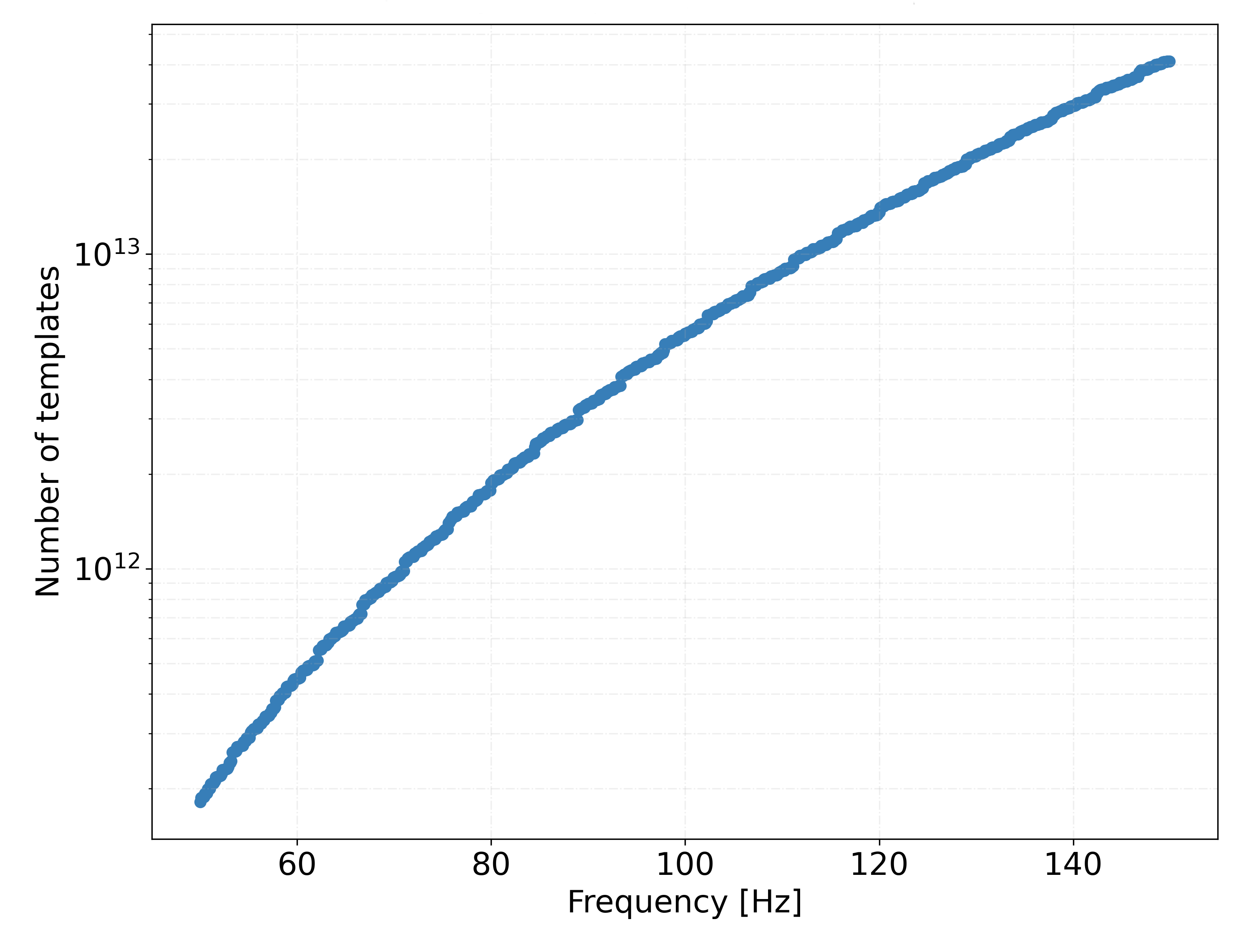
Figure 3: Number of templates searched in each 0.1 Hz frequency band as a function of frequency. The total number of templates is $\sim 1.05\times 10^{16}$.

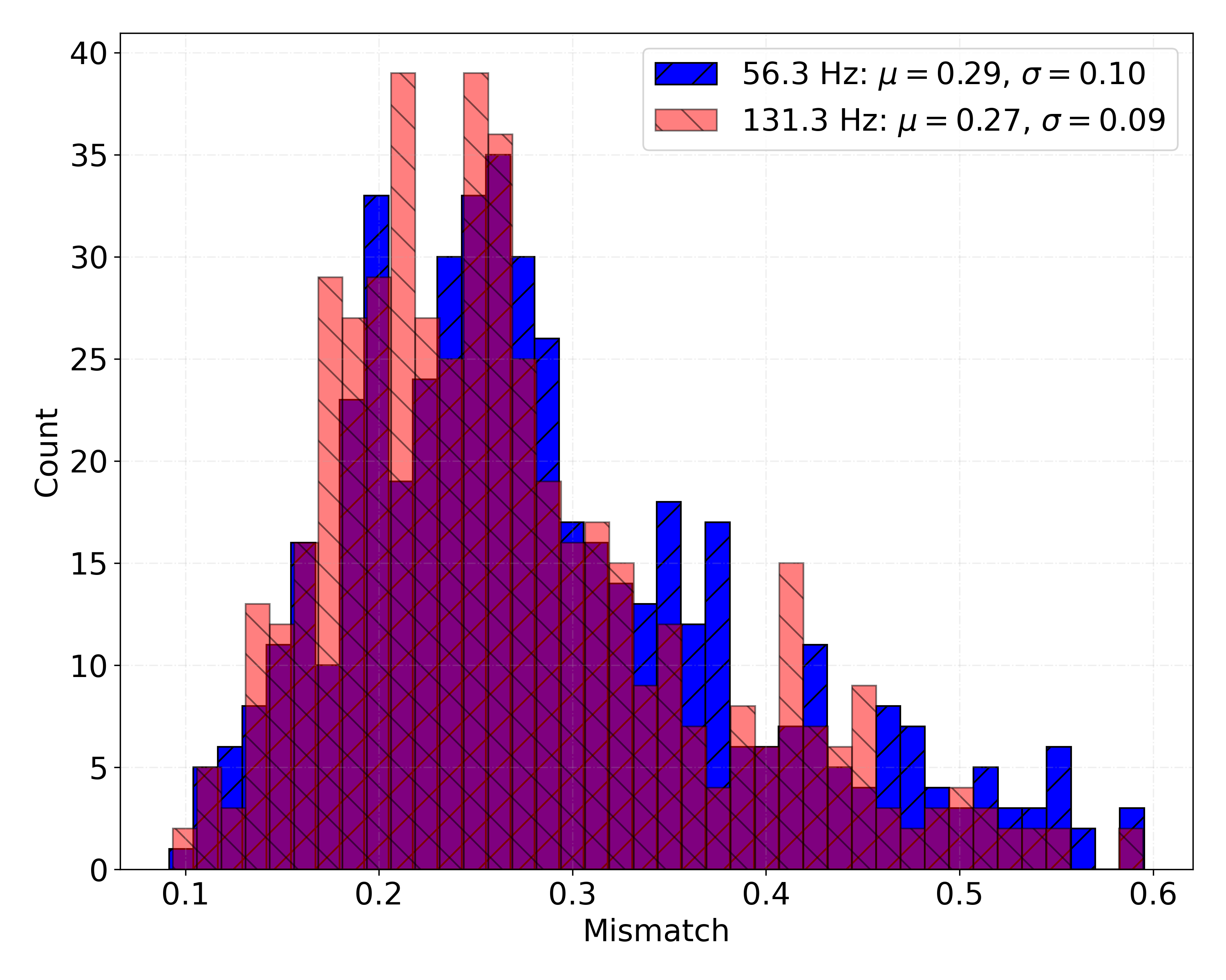
Figure 4: Mismatch distribution of this search at two different 0.1 Hz frequency bands, with the other parameters that describe the continuous wave signal spanning the ranges given in Table 1. The legend shows the mean and standard deviation of each distribution.

3.5 Candidate selection

We divide each 0.1 Hz band in 5 mHz sub-bands and consider the $10^{6}$ templates with the highest significance $s$ in every sub-band. Compared to previous searches we have not picked the top candidates directly from the 0.1 Hz bands because the low-frequency region is affected by very loud but narrow spectral disturbances, whose contamination can be effectively contained by simply choosing the top candidates in smaller bands. Figure 5 shows the significance $s$ of the top template in each 5 mHz sub-band.

We use the clustering procedure of Covas & Sintes (2019, 2020) to group together results attributed to the same origin. The cluster with the highest significance per 5 mHz band is saved for further analysis, yielding a total of 20 000 clusters. In what follows we refer to these selected clusters as candidates.

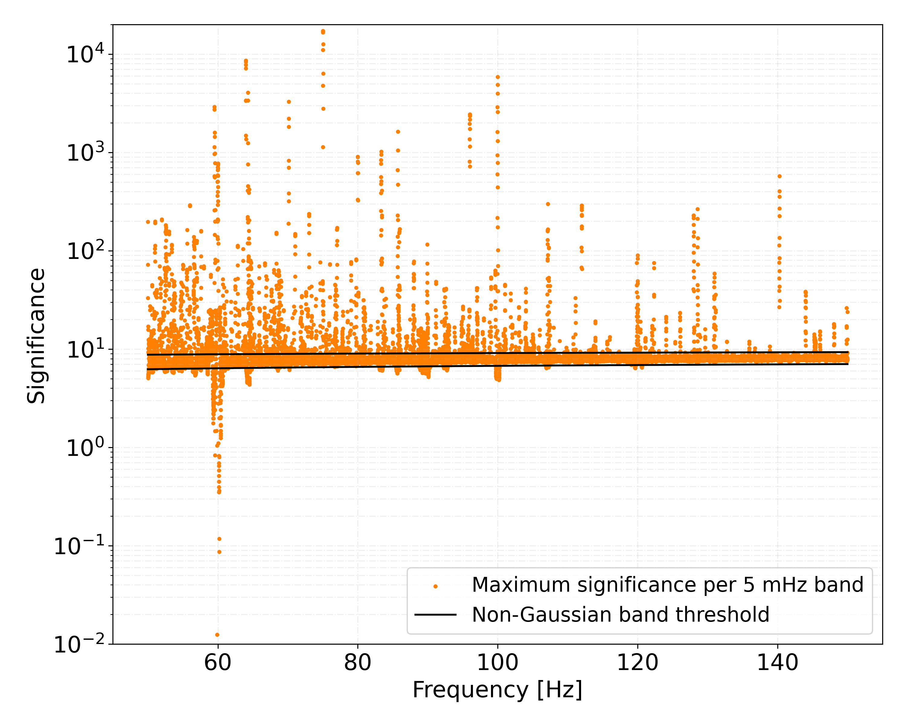
Figure 5: Maximum significance $s$ in each 5 mHz frequency sub-band as a function of frequency. Significance values well below the average level are due to spectral disturbances that lead to an “under-weighing” of the data from various normalization procedures and produce low values of the detection statistic. The black lines are used to determine the frequency bands where the upper limits apply, see Section 4.1.

Before analyzing the candidates with a longer coherence time, we check whether they might be due to a line. We do this by computing the $\log_{10}\hat{B}_{\mathrm{S/GLtL}}$ statistic of Keitel (2016) with $\hat{\mathcal{F}}_{*}=0$. This effectively results in a comparison between the multi-detector and the largest of the single-detector $\mathcal{F}$-statistic values. For astrophysical signals we expect the multi-detector statistic to be larger than the single-detector. We calibrate the veto based on injected signals from our target population added to the real data (we only use signals that generate a cluster with a higher significance than the top cluster in their respective 5 mHz band), as illustrated in Figure 6. This veto has a false dismissal probability of less than 0.004%. Applied to our 20 000 candidates, it removes 1 718, leaving 18 282 candidates for the next stage.

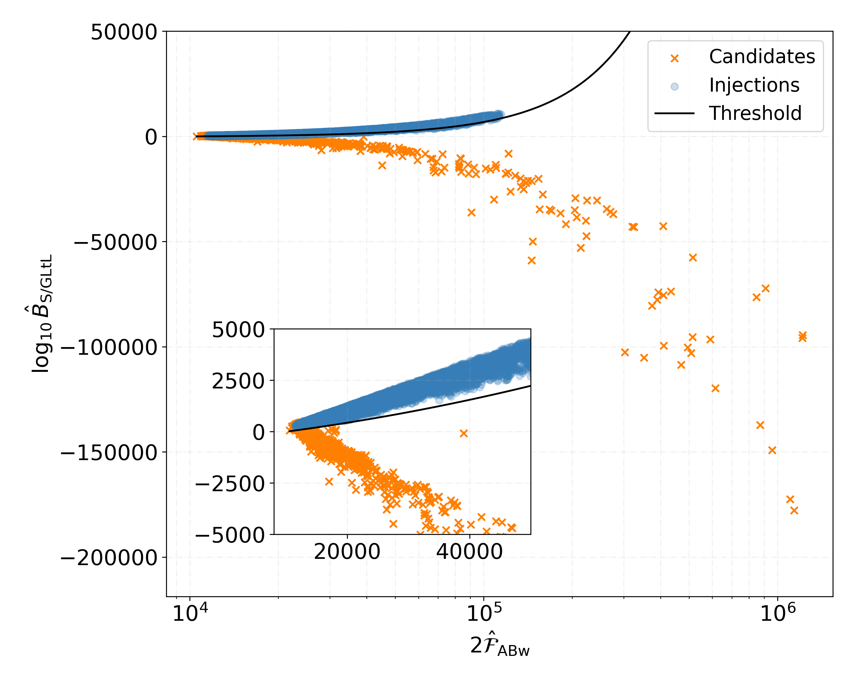
Figure 6: Distribution of $\log_{10}\hat{B}_{\mathrm{S/GLtL}}$ values as a function of $2\hat{\mathcal{F}}_{\mathrm{ABw}}$ for 25 673 injected signals from our target population (shown with blue circles) and 20 000 candidates (shown with orange crosses). The black line shows the threshold. The upper region is the candidate acceptance region.

3.6 Follow-up

In the next step we apply a follow-up procedure where the coherence time $T_{\textrm{coh}}$ is increased, and use a nested sampling algorithm (Ashton et al., 2019) to calculate the detection statistic (Covas et al., 2024). Due to the increased coherence time, the follow-up resolves different values of the frequency derivative, eccentricity, and argument of periapsis, which are now searched for explicitly in the ranges given by Table 1. We use the injected signals from our target population to determine the search region (Covas et al., 2024).

If a candidate is due to a gravitational-wave signal we expect that its significance will increase through the different stages. Candidates from stage $i$ are discarded if their significance $s_{i}$ does not increase with respect to $s_{0}$ as expected for astrophysical signals. We calibrate this expectation with our target signal population, as shown in Figure 7.

Only two follow-up stages are necessary to discard all candidates:

• Stage 1: $T_{\mathrm{coh}}=45\,000$ s with a significance-veto false dismissal of $\simeq 0.3\%$ (see left plot of Figure 7). This results in 458 surviving candidates out of 18 282.

• Stage 2: $T_{\mathrm{coh}}=135\,000$ s with a significance-veto false dismissal of $<0.1\%$ (see right plot of Figure 7). This results in $24+1$ surviving candidates out of 458.

• $\hat{B}_{\mathrm{S/GLtL}}$ veto with a false dismissal of $<0.1\%$ (see Figure 8). Only the “+1” candidate (which is a hardware-injected signal) survives out of the $24+1$.

The two candidates with the largest significances $s_{2}$ are at $\sim 52.8$ Hz and $\sim 145.4$ Hz and can be associated with hardware injections – signals added to the data in hardware for pipeline validation purposes (Biwer et al., 2017). Despite these signals being from isolated neutron stars rather than in binary systems we still recover them, because they are very loud. Three such signals are actually present in the frequency range covered by this search and we recover the loudest two. The $\sim 145.4$ Hz candidate is actually below our threshold, but it is so close to the threshold and so significant that we would have followed it up anyways. It is the “+1” candidate that we previously refer to.

To investigate the nature of the surviving candidates we compute the line-robust statistic $\log_{10}\hat{B}_{\mathrm{S/GLtL}}$ with $\hat{\mathcal{F}}_{*}=0$ as previously done, and compare it with what is expected from the target signal population as a function of $s_{0}$. The result is shown in Figure 8. The $\sim 145.4$ Hz candidate survives while all other are vetoed. Based on these results we conclude that none of our candidates can be associated with a real continuous wave signal.

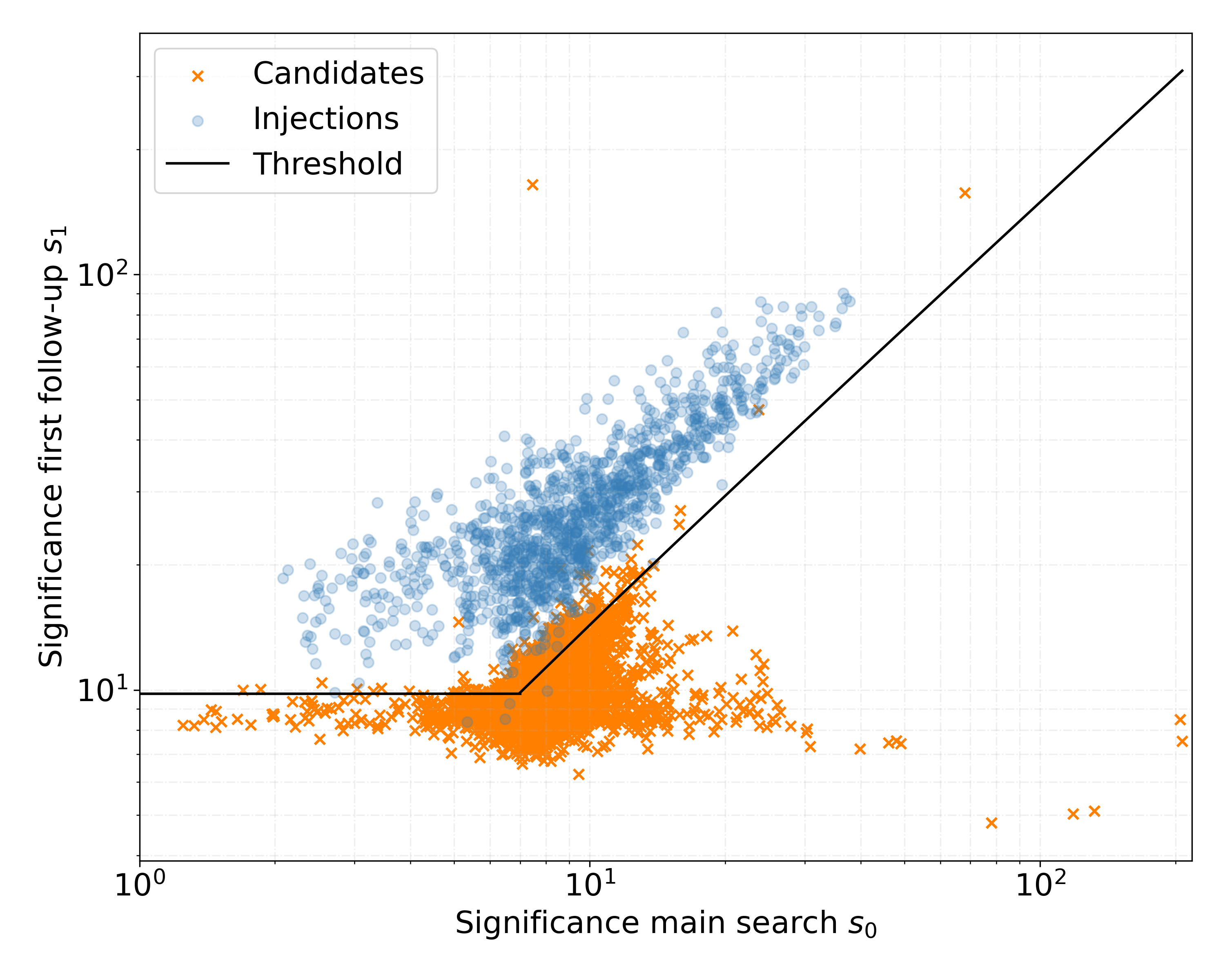
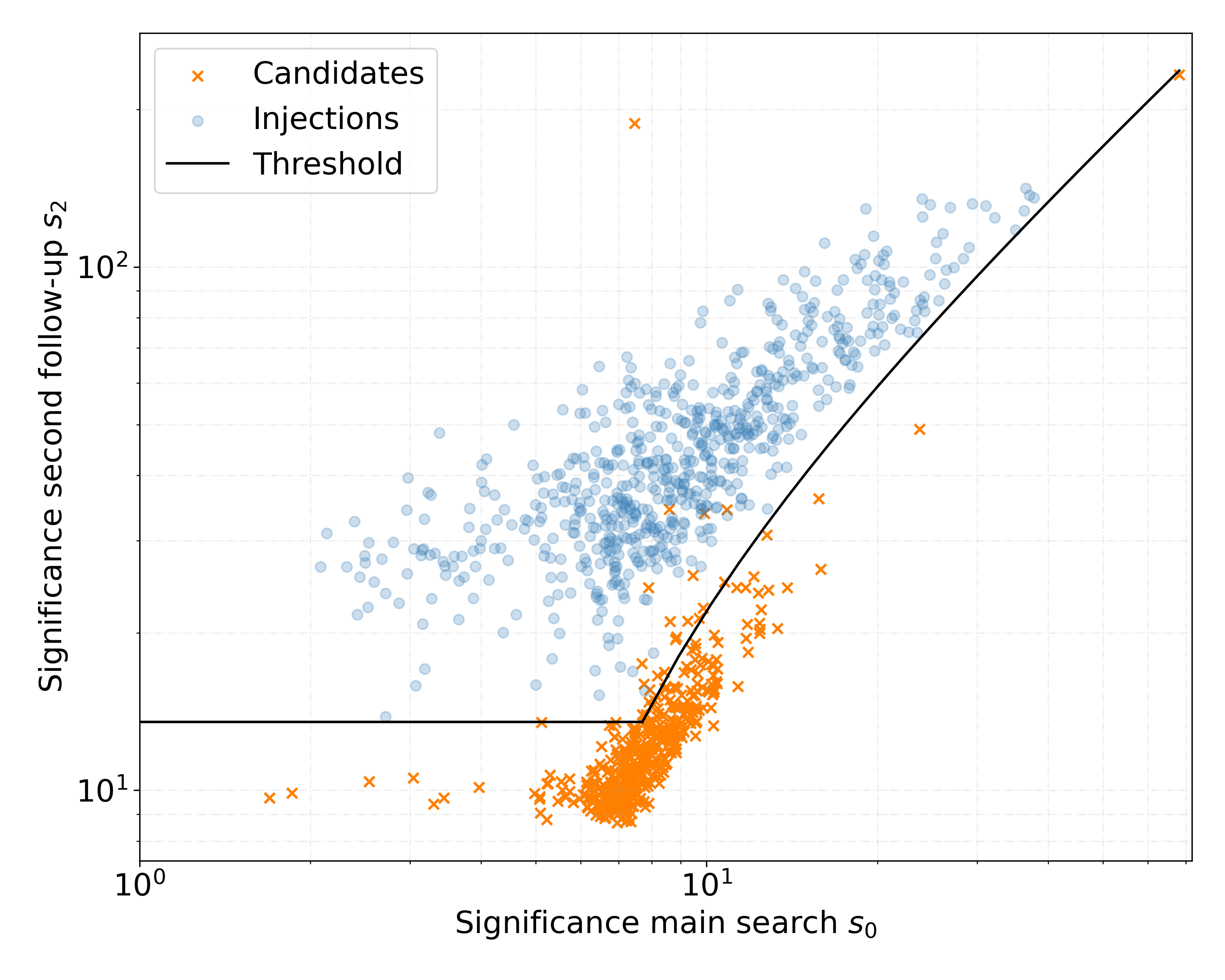
Figure 7: Orange crosses: significance of search candidates in stage 1 ($s_{1}$, left plot) and in stage 2 ($s_{2}$, right plot) as a function of their significance in stage 0 ($s_{0}$). Stage 1 investigates 18 282 candidates. Stage 2 investigates 458 candidates. Blue crosses: target signal population with 1 288 signals investigated by stage 1 of which 1 284 survive and are investigated in stage 2. The candidate survival region is the region above the black line.

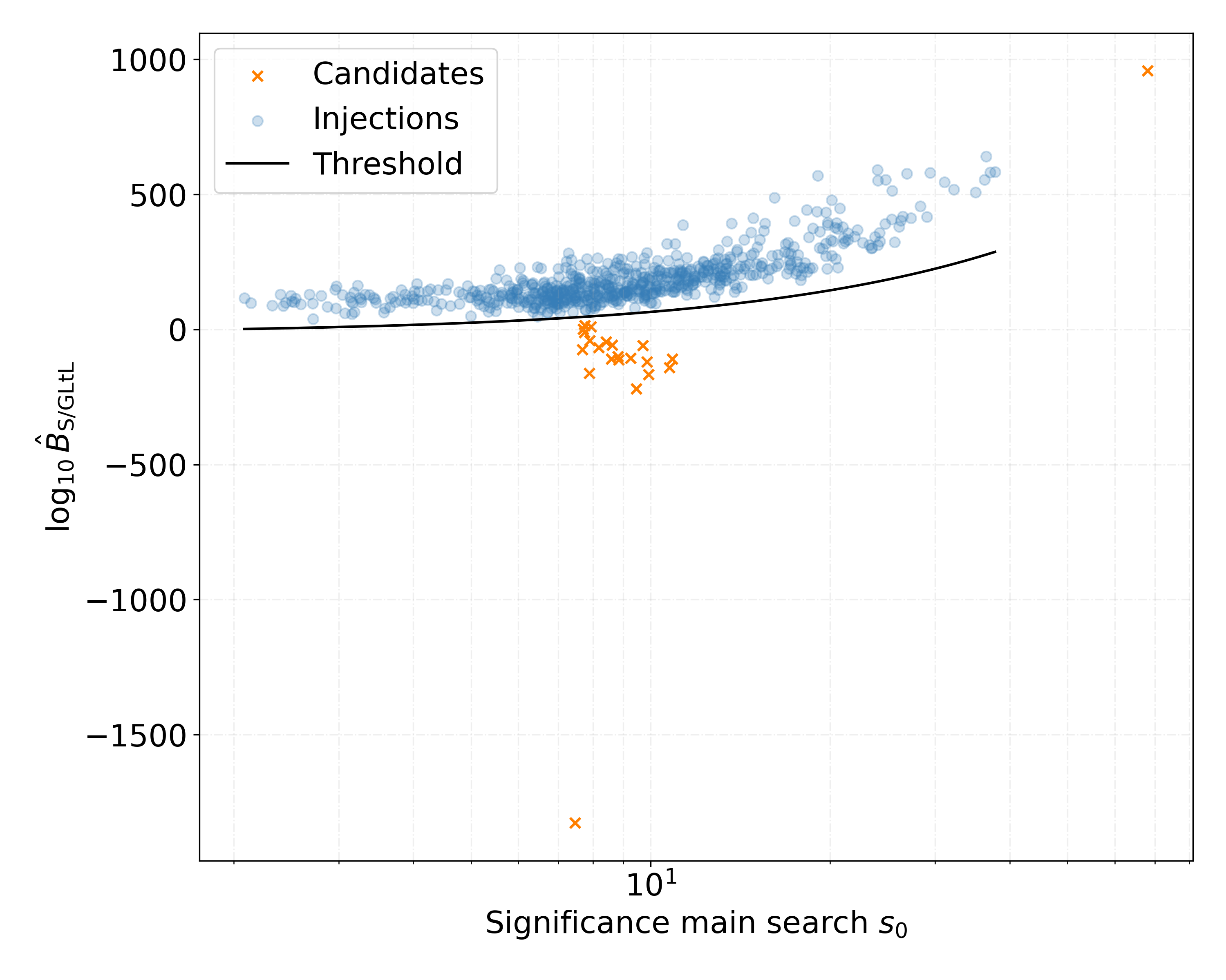
Figure 8: $\log_{10}\hat{B}_{\mathrm{S/GLtL}}$ values of the stage 2 candidates as a function of the stage 0 significance $s_{0}$. Blue circles: 1 284 injected signals from the target signal population. Orange crosses: 24 surviving candidates from stage 2 plus the high-significance candidate at the upper right corner of the right plot in Figure 7. The candidate survival region is the region above the black line.

4 Results

4.1 Upper limits

We calculate the 95%-confidence upper limits on the gravitational-wave amplitude $h_{0}^{95\%}(f)$ in every 0.1 Hz band. This is the amplitude such that 95% of a population of signals with that amplitude, frequency in that band, and with the same distribution as our target population, would have survived our pipeline. This means that these signals generate a cluster with a higher significance than the top cluster in the respective 5 mHz band, and the candidate passes the two stages of the follow-up and the $\hat{B}_{\mathrm{S/GLtL}}$ vetoes.

We determine the upper limits in the ten 0.1 Hz bands mentioned in Section 3.3. For each band and $h_{0}$ value we compute the fraction of detected signals out of a total of $250$ from our target population. We determine the $h_{0}$ corresponding to 95% detection efficiency with a linear interpolation, as shown in Figure 9.

We associate to every upper limit a sensitivity depth ${\mathcal{D}}$ (Behnke et al., 2015; Dreissigacker et al., 2018), defined as

$${\mathcal{D}}^{95\%}(f)=\frac{\sqrt{S_{\mathrm{n}}(f)}}{h_{0}^{95\%}(f)},$$ (7)

where $\sqrt{S_{\mathrm{n}}(f)}$ is the amplitude spectral density of the data, shown in Figure 1 with the middle green curve. Across the ten different bands the average 95% sensitivity depth is $38.6\pm 0.9$ $\textrm{Hz}^{-1/2}$, with $1\sigma$ uncertainty. We use this value inverting Equation (7) to determine the upper limits $h_{0}^{95\%}$ in the other frequency bands. This will yield correct upper limit estimates as long as the noise is not affected by large disturbances.

We identify the 5 mHz sub-bands where the noise may be affected by large disturbances by looking at the significance of the loudest candidate. If it is too far (12 standard deviations) on the tails of the distribution in quiet bands, the upper limit does not hold in that sub-band (Covas & Sintes, 2020). The black lines shown in Figure 5 bracket the interval of significance values that define the accepted bands.

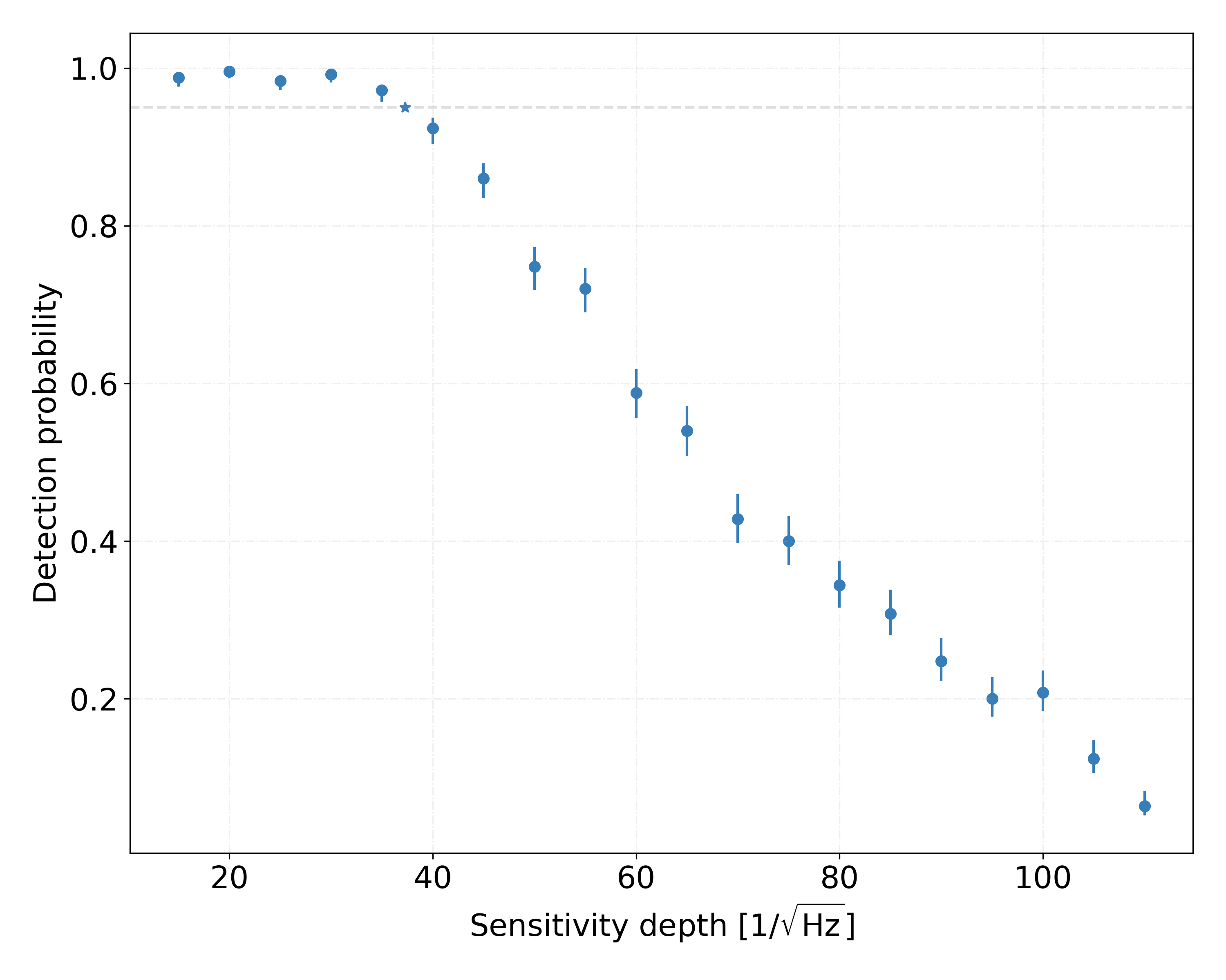
Figure 9: Detection probability as a function of the sensitivity depth $\sqrt{S_{n}(f_{0})}/h_{0}$ of different signals with frequency $f_{0}$ (distributed as $f_{0}\in 85.55\pm 0.05$ Hz) and amplitude $h_{0}$. The error bars show the $1\sigma$ uncertainty, and the star marks the interpolated detection probability at $\mathcal{D}^{95\%}$.

The upper limit values and the list of frequency bands where the upper limits do not apply are available in machine-readable format in the supplementary materials and shown in Figure 10. The most stringent upper limit is $1.25\times 10^{-25}$ at $144.32$ Hz.

The search of Abbott et al. (2021) achieves a sensitivity depth of $\sim 22.5$ $\textrm{Hz}^{-1/2}$ at similar frequencies, which is a factor $\sim 1.75$ times less sensitive than our result. We estimate that part of this additional sensitivity is due to our search using the entire O3 dataset, rather than just the first half as in Abbott et al. (2021). This accounts for a factor $\sim 2^{1/4}=1.2$. The rest comes from the search being intrinsically more sensitive.

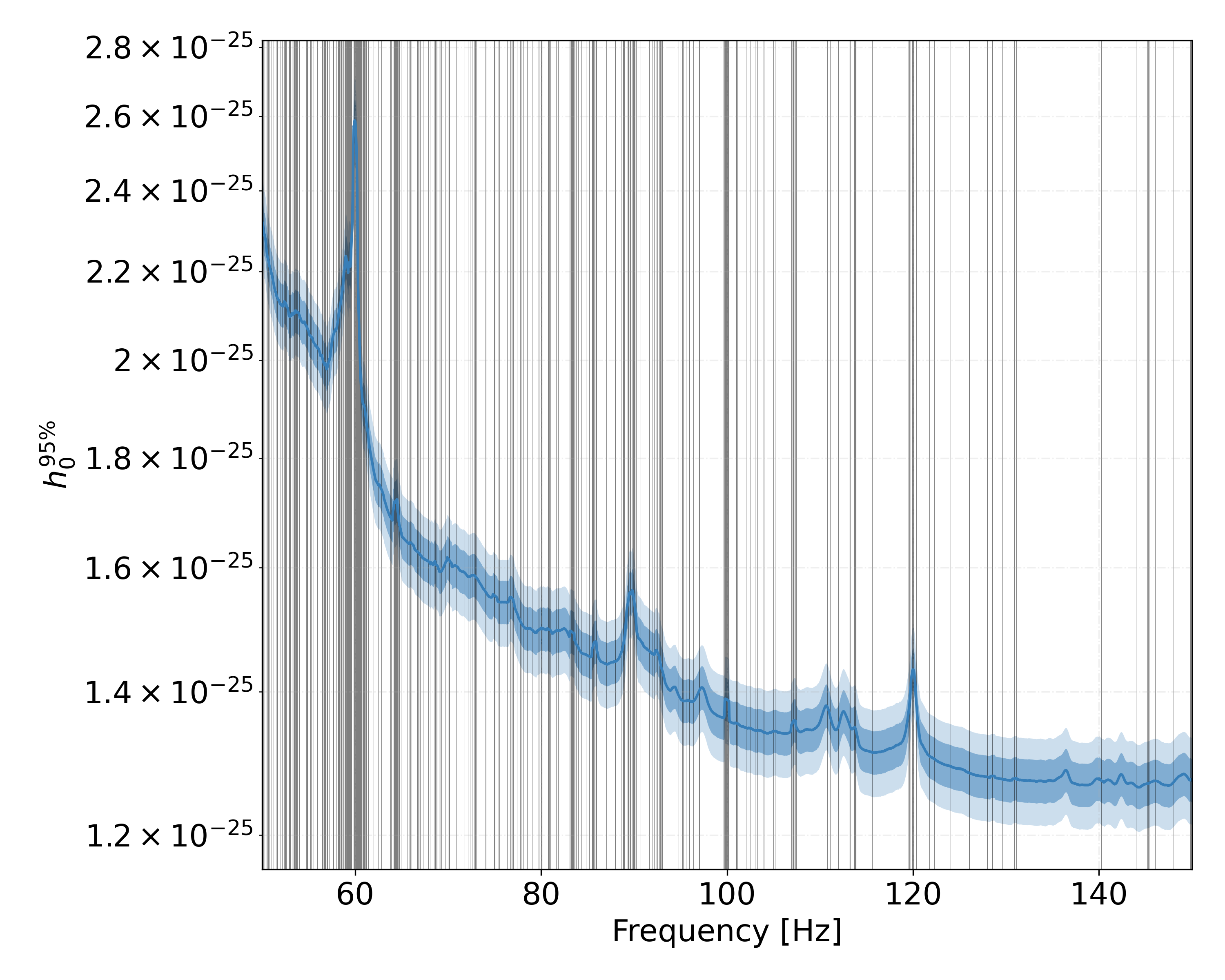
Figure 10: Upper limits on the gravitational-wave amplitude $h_{0}^{95\%}$ at the $95\%$ confidence level as a function of frequency. The shaded areas surrounding the curve indicate the $1\sigma$ and $2\sigma$ uncertainty regions. The vertical black rectangles show the $3\,402$ (out of $20\,000$) 5 mHz frequency bands where the upper limits do not apply.

If the continuous waves are sourced by an equatorial elliptiticty $\epsilon=|I_{xx}-I_{yy}|/I_{zz}$, with $I_{zz}$ being the moment of inertia of the star with respect to the principal axis aligned with the rotational axis, the gravitational-wave amplitude at a distance $d$ is

$$h_{0}=10^{-26}\left[\frac{I_{zz}}{10^{38}\mathrm{~{}kg~{}m}^{2}}\right]\left[\frac{\epsilon}{10^{-6}}\right]\left[\frac{f_{0}}{100\mathrm{~{}Hz}}\right]^{2}\left[\frac{1\mathrm{~{}kpc}}{d}\right].$$ (8)

The upper limits on $h_{0}$ can be used to calculate upper limits on the asymmetry of the targeted neutron star population by rearranging Equation 8. These ellipticity upper limits depend on the moment of inertia of the neutron star, which is uncertain by around a factor of three (see Section 4B of Abbott et al., 2007), although more exotic neutron star models such as quark stars or lower-mass neutron stars could have even higher moments of inertia (Horowitz, 2010; Owen, 2005). Figure 11 shows these results at three different distances and two values of the moment of inertia.

These upper limits on the ellipticity are the most restrictive to date for unknown neutron stars in binary systems. For sources at 1 kpc, with $I_{zz}=10^{38}$ kg m² and emitting continuous waves at 150 Hz, the ellipticity can be constrained to be $<5.2\times 10^{-6}$, while at 10 pc we have $\epsilon<5.2\times 10^{-8}$. If instead we assume $I_{zz}=3\times 10^{38}$ kg m² (as could be due to an equation of state that supports neutron stars with $\approx 70\%$ larger radii), the upper limits are more stringent, as shown by the dashed traces. For example, at 100 pc and 100 Hz, the upper limit is $\epsilon<4\times 10^{-7}$. If the true minimum ellipticity is $10^{-9}$ as suggested by Woan et al. (2018), we are about one order of magnitude above that limit for neutron stars at 10 pc and 150 Hz, and two orders of magnitude for stars at 100 pc.

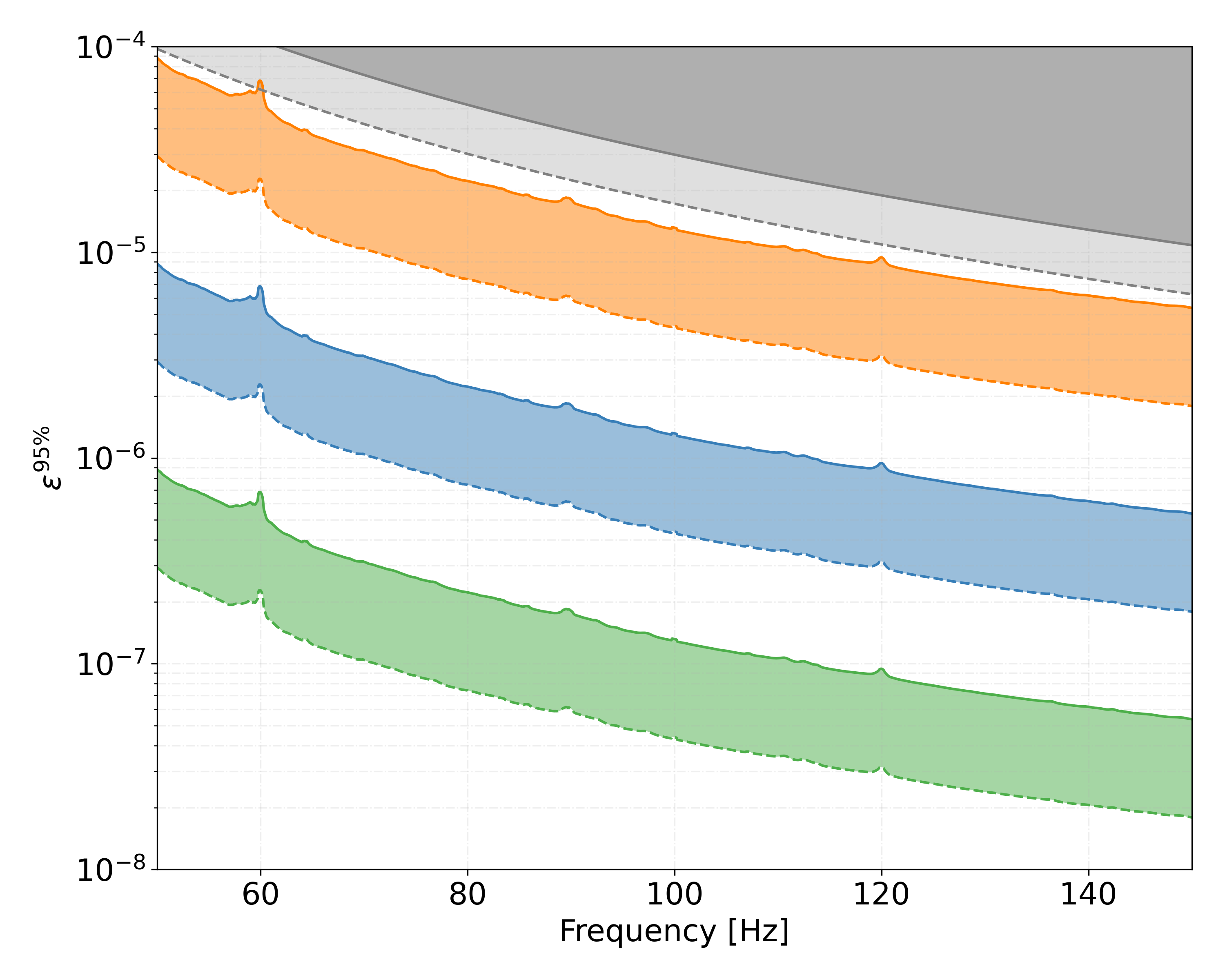
Figure 11: Upper limits on the neutron star ellipticity $\epsilon$ at the $95\%$ confidence level as a function of frequency. The three different colors show results for distances of 1 kpc (upper orange curves), 100 pc (middle blue curves), and 10 pc (green bottom curves). The dashed lines use a moment of inertia of $I_{zz}=3\times 10^{38}$ kg m² instead of the canonical $I_{zz}=10^{38}$ kg m² value, used by the solid lines. The upper shaded gray area shows the region where this search is not sensitive because the high ellipticities would generate a spin-down larger than the one probed by this search.

If the continuous waves are sourced by r-modes, the gravitational-wave amplitude is given by (Owen, 2010)

$$h_{0}= 10^{-26}\left[\frac{\alpha}{2.8\times 10^{-4}}\right]\left[\frac{100\mathrm{~{}Hz}}{f_{0}}\right]^{3}\left[\frac{d}{1\mathrm{~{}kpc}}\right]$$ (9)

$$\times\left[\frac{1.4~{}{\mathrm{M}}_{\odot}}{M}\right]\left[\frac{11.7~{}{\mathrm{km}}}{R}\right]^{3},$$

where $\alpha$ is the r-mode amplitude, $M$ is the mass of the neutron star, and $R$ its radius.

The upper limits on $h_{0}$ can be used to calculate upper limits on the r-mode amplitude of the targeted neutron star population by rearranging Equation 9. These r-mode amplitude upper limits depend on the neutron star mass and radius (connected by the unknown equation of state). Figure 12 shows these results at three different distances and two mass-radius combinations.

For sources at 1 kpc, with $M=1.4~{}M_{\odot}$, $R=11.7$ km and emitting continuous waves at 150 Hz, the r-mode amplitude can be constrained at $\alpha<10^{-3}$, while at 10 pc we have $\alpha<10^{-5}$. If instead we assume $M=1.4~{}M_{\odot}$ and $R=11.7$ km, the upper limits are more stringent, as shown by the dashed traces. For example, at 100 pc and 100 Hz, the upper limit is $\alpha<2\times 10^{-4}$. The range of theoretical predictions in the literature on r-mode amplitudes is $\alpha\sim 8\times 10^{-7}-10^{-4}$ (Gusakov et al., 2014a, b) or $\alpha\sim 10^{-5}$ (Bondarescu et al., 2007). It can be seen that for neutron stars between 10 and 100 pc, our results start to constrain the upper limits of these theoretical ranges.

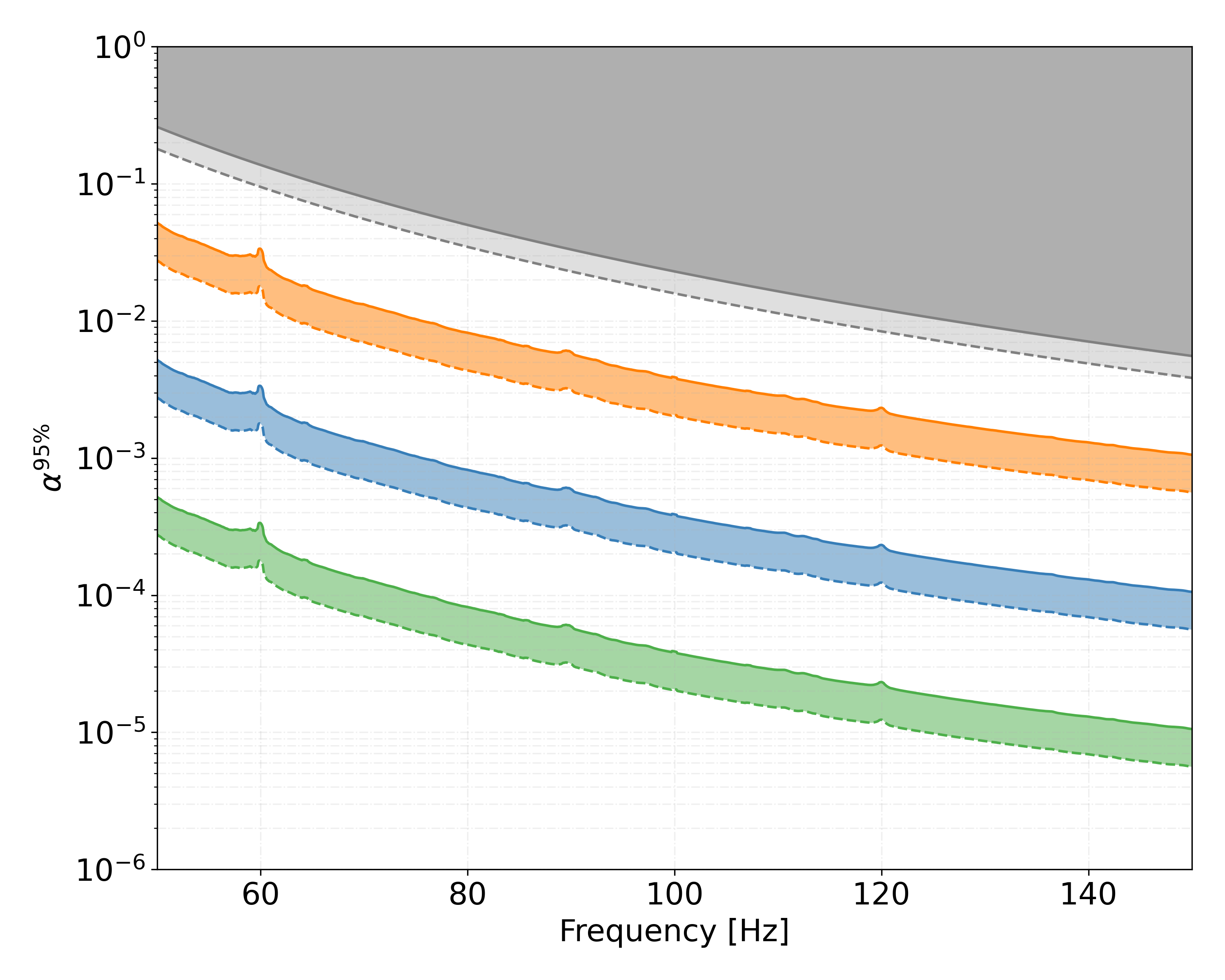
Figure 12: Upper limits on the r-mode amplitude $\alpha$ at the $95\%$ confidence level as a function of frequency. The three different colors show results for distances of 1 kpc (upper orange curves), 100 pc (middle blue curves), and 10 pc (green bottom curves). The dashed lines assume $M=1.9~{}M_{\odot}$ and $R=13$ km, while the solid lines assume $M=1.4~{}M_{\odot}$ and $R=11.7$ km. The upper shaded gray area shows the region where this search is not sensitive because the high r-mode amplitudes would generate a spin-down larger than the one probed by this search.

5 Conclusions

In this paper we have presented results from a direct search for continuous gravitational waves from neutron stars in binary systems with the largest orbital periods and widest orbits ever directly investigated. We set the most constraining direct upper limits in the investigated region of parameter space, improving on existing direct upper limits in a similar frequency region by about $75\%$.

This search exemplifies the capabilities of the newly developed BinarySkyHou$\mathcal{F}$ pipeline, thanks to the usage of a longer coherence time, a more sensitive detection statistic, and finer parameter space grids in both the coherent and semi-coherent grids. The search took $\sim 82\,000$ CPU-hours to complete, running on a combination of Intel(R) Xeon(R) Platinum 8360Y @ 2.40GHz CPUs and NVIDIA A100-SXM4-40GB GPUs.

Singh et al. (2019) proposed that searches for continuous waves from isolated neutron stars also probe signals from neutron stars in high orbital period binary systems with small eccentricity. They applied this idea to the null results of a search for continuous waves from isolated neutron stars (Steltner et al., 2021) and, under those assumptions, constrained the gravitational wave amplitude with a remarkable sensitivity depth of $\sim 50$ Hz^-1/2. Their $(P_{\mathrm{orb}},a_{\mathrm{p}})$ parameter range partly overlaps the parameter space that we have investigated here, as shown in Figure 2. Their investigation is however not a direct search and can only recast a null result to the binary parameter space, or re-interpret a detection ascribed to an isolated system as coming from a binary. Conversely, the search presented here could detect a new signal.

References

- Aasi et al. (2014) Aasi, J., et al. 2014, Phys. Rev. D., 90, 062010, doi: 10.1103/PhysRevD.90.062010
- Aasi et al. (2015) —. 2015, Class. Quant. Grav., 32, 074001, doi: 10.1088/0264-9381/32/7/074001
- Abbott et al. (2007) Abbott, B., et al. 2007, Phys. Rev. D., 76, 042001, doi: 10.1103/PhysRevD.76.042001
- Abbott et al. (2021) Abbott, R., et al. 2021, Phys. Rev. D., 103, 064017, doi: 10.1103/PhysRevD.103.064017
- Abbott et al. (2022a) —. 2022a, Phys. Rev. D, 106, 102008, doi: 10.1103/PhysRevD.106.102008
- Abbott et al. (2022b) —. 2022b, Phys. Rev. D, 106, 102008, doi: 10.1103/PhysRevD.106.102008
- Abbott et al. (2023a) —. 2023a, Phys. Rev. D, 108, 069901, doi: 10.1103/PhysRevD.108.069901
- Abbott et al. (2023b) —. 2023b, Astrophys. J. Supplement Series, 267, 29, doi: 10.3847/1538-4365/acdc9f
- Allen & Mendell (2004) Allen, B., & Mendell, G. 2004, SFT (Short-Time Fourier Transform) Data Format Version 2 Specification, Tech. Rep. T040164, LIGO DCC. https://dcc.ligo.org/LIGO-T040164/public
- Ashton et al. (2019) Ashton, G., Hübner, M., Lasky, P., Talbot, C., et al. 2019, Astrophys. J. Supplement Series, 241, 27, doi: 10.3847/1538-4365/ab06fc
- Ashton et al. (2015) Ashton, G., Jones, D. I., & Prix, R. 2015, Phys. Rev. D, 91, 062009, doi: 10.1103/PhysRevD.91.062009
- Ashton et al. (2017) Ashton, G., Prix, R., & Jones, D. I. 2017, Phys. Rev. D, 96, 063004, doi: 10.1103/PhysRevD.96.063004
- Behnke et al. (2015) Behnke, B., Papa, M. A., & Prix, R. 2015, Phys. Rev. D., 91, 064007, doi: 10.1103/PhysRevD.91.064007
- Biwer et al. (2017) Biwer, C., Barker, D., Batch, J. C., et al. 2017, Phys. Rev. D, 95, 062002, doi: 10.1103/PhysRevD.95.062002
- Bondarescu et al. (2007) Bondarescu, R., Teukolsky, S. A., & Wasserman, I. 2007, Phys. Rev. D., 76, 064019, doi: 10.1103/PhysRevD.76.064019
- Covas et al. (2022) Covas, P. B., Papa, M. A., Prix, R., & Owen, B. J. 2022, The Astrophysical Journal Letters, 929, L19, doi: 10.3847/2041-8213/ac62d7
- Covas & Prix (2022a) Covas, P. B., & Prix, R. 2022a, Phys. Rev. D, 106, 084035, doi: 10.1103/PhysRevD.106.084035
- Covas & Prix (2022b) —. 2022b, Phys. Rev. D, 105, 124007, doi: 10.1103/PhysRevD.105.124007
- Covas et al. (2024) Covas, P. B., Prix, R., & Martins, J. 2024, Phys. Rev. D, 110, 024053, doi: 10.1103/PhysRevD.110.024053
- Covas & Sintes (2020) Covas, P. B., & Sintes, A. 2020, Phys. Rev. Lett., 124, 191102, doi: 10.1103/PhysRevLett.124.191102
- Covas & Sintes (2019) Covas, P. B., & Sintes, A. M. 2019, Phys. Rev. D., 99, 124019, doi: 10.1103/PhysRevD.99.124019
- Covas et al. (2018) Covas, P. B., et al. 2018, Phys. Rev. D, 97, 082002, doi: 10.1103/PhysRevD.97.082002
- Davis et al. (2019) Davis, D., Massinger, T. J., Lundgren, A. P., et al. 2019, Class. Quant. Grav., 36, 055011, doi: 10.1088/1361-6382/ab01c5
- Dergachev & Papa (2023) Dergachev, V., & Papa, M. A. 2023, Phys. Rev. X, 13, 021020, doi: 10.1103/PhysRevX.13.021020
- Dreissigacker et al. (2018) Dreissigacker, C., Prix, R., & Wette, K. 2018, Phys. Rev. D., 98, 084058, doi: 10.1103/PhysRevD.98.084058
- Gusakov et al. (2014a) Gusakov, M. E., Chugunov, A. I., & Kantor, E. M. 2014a, Phys. Rev. Lett., 112, 151101, doi: 10.1103/PhysRevLett.112.151101
- Gusakov et al. (2014b) —. 2014b, Phys. Rev. D., 90, 063001, doi: 10.1103/PhysRevD.90.063001
- Horowitz (2010) Horowitz, C. J. 2010, Phys. Rev. D., 81, 103001, doi: 10.1103/PhysRevD.81.103001
- Jaranowski et al. (1998) Jaranowski, P., et al. 1998, Phys. Rev. D., 58, 063001, doi: 10.1103/PhysRevD.58.063001
- Jones & Riles (2024) Jones, D. I., & Riles, K. 2024, Multimessenger observations and the science enabled: Continuous waves and their progenitors, equation of state of dense matter. https://arxiv.org/abs/2403.02066
- Keitel (2016) Keitel, D. 2016, Phys. Rev. D, 93, 084024, doi: 10.1103/PhysRevD.93.084024
- Krishnan et al. (2004) Krishnan, B., et al. 2004, Phys. Rev. D., 70, 082001, doi: 10.1103/PhysRevD.70.082001
- Leaci & Prix (2015) Leaci, P., & Prix, R. 2015, Phys. Rev. D, 91, 102003, doi: 10.1103/PhysRevD.91.102003
- LIGO, Virgo, KAGRA collaborations (2021a) LIGO, Virgo, KAGRA collaborations. 2021a, The O3a Data Release, doi: 10.7935/nfnt-hm34
- LIGO, Virgo, KAGRA collaborations (2021b) —. 2021b, The O3b Data Release, doi: 10.7935/pr1e-j706
- Manchester et al. (2005) Manchester, R. N., Hobbs, G. B., Teoh, A., & Hobbs, M. 2005, Astronom. J., 129, 1993–2006, doi: 10.1086/428488
- Mukherjee et al. (2018) Mukherjee, A., Messenger, C., & Riles, K. 2018, Phys. Rev. D., 97, 043016, doi: 10.1103/PhysRevD.97.043016
- Owen (2005) Owen, B. J. 2005, Phys. Rev. Lett., 95, 211101, doi: 10.1103/PhysRevLett.95.211101
- Owen (2010) —. 2010, Phys. Rev. D., 82, 104002, doi: 10.1103/PhysRevD.82.104002
- Riles (2023) Riles, K. 2023, Liv. Rev. in Relat., 26, 1, doi: 10.1007/s41114-023-00044-3
- Singh (2017) Singh, A. 2017, Phys. Rev. D, 95, 024022, doi: 10.1103/PhysRevD.95.024022
- Singh & Papa (2023) Singh, A., & Papa, M. A. 2023, Astrophys. J., 943, 99, doi: 10.3847/1538-4357/acaf80
- Singh et al. (2019) Singh, A., Papa, M. A., & Dergachev, V. 2019, Phys. Rev. D, 100, 024058, doi: 10.1103/PhysRevD.100.024058
- Steltner et al. (2022) Steltner, B., Papa, M., & Eggenstein, H.-B. 2022, Phys. Rev. D., 105, 022005, doi: 10.1103/PhysRevD.105.022005
- Steltner et al. (2023) Steltner, B., Papa, M. A., Eggenstein, H.-B., et al. 2023, Astrophys. J., 952, 55, doi: 10.3847/1538-4357/acdad4
- Steltner et al. (2021) Steltner, B., et al. 2021, Astrophys. J., 909, 79, doi: 10.3847/1538-4357/abc7c9
- Tenorio et al. (2021) Tenorio, R., Keitel, D., & Sintes, A. M. 2021, Universe, 7, 474, doi: 10.3390/universe7120474
- Wette (2023) Wette, K. 2023, Astroparticle Physics, 153, 102880, doi: https://doi.org/10.1016/j.astropartphys.2023.102880
- Woan et al. (2018) Woan, G., et al. 2018, Astrophys. J., 863, L40, doi: 10.3847/2041-8213/aad86a