TiM4Rec: An Efficient Sequential Recommendation Model Based on Time-Aware Structured State Space Duality Model

Abstract.

Sequential recommendation represents a pivotal branch of recommendation systems, centered around dynamically analyzing the sequential dependencies between user preferences and their interactive behaviors. Despite the Transformer architecture-based models achieving commendable performance within this domain, their quadratic computational complexity relative to the sequence dimension impedes efficient modeling. In response, the innovative Mamba architecture, characterized by linear computational complexity, has emerged. Mamba4Rec further pioneers the application of Mamba in sequential recommendation. Nonetheless, Mamba 1’s hardware-aware algorithm struggles to efficiently leverage modern matrix computational units, which lead to the proposal of the improved State Space Duality (SSD), also known as Mamba 2. While the SSD4Rec successfully adapts the SSD architecture for sequential recommendation, showing promising results in high-dimensional contexts, it suffers significant performance drops in low-dimensional scenarios crucial for pure ID sequential recommendation tasks. Addressing this challenge, we propose a novel sequential recommendation backbone model, TiM4Rec, which ameliorates the low-dimensional performance loss of the SSD architecture while preserving its computational efficiency. Drawing inspiration from TiSASRec, we develop a time-aware enhancement method tailored for the linear computation demands of the SSD architecture, thereby enhancing its adaptability and achieving state-of-the-art (SOTA) performance in both low and high-dimensional modeling. The code for our model is publicly accessible at https://github.com/AlwaysFHao/TiM4Rec.

1. Introduction

Sequential recommendation represents a predictive technology that leverages user’s historical interaction sequence. Unlike traditional recommendation methods—such as collaborative filtering and content based filtering—which rely heavily on static user features and historical behavior, it emphasizes capturing dynamic user behavior characteristic, which is more adept at accommodating rapid shifts in user interests and diverse consumption patterns.

The landscape of sequential recommendation models has evolved significantly, transitioning from early models based on Markov chains (fpmc; hrm) to those leveraging CNNs (tang2018personalized), RNNs (li2017neural; GRU4Rec), GNNs (srgnn; chang2021sequential), notable examples include Caser (tang2018personalized) and GRU4Rec (GRU4Rec). However, these models often suffer from performance limitations inherent to their core architectures, resulting in suboptimal prediction accuracy. The introduction of the Transformer (vaswani2017attention) architecture, grounded in an attention mechanism, has marked a paradigm shift due to its superior performance and parallelizable training capabilities, making it a mainstream framework across various domains that has also significantly influenced the sequential recommendation domain. In recent years, as evidenced by models like SASRec (kang2018self) and BERT4Rec (sun2019bert4rec) effectively adapting the success of Transformers to this area.

Despite their advancements, these early Transformer-based models did not sufficiently account for the unique data characteristics, notably the temporal shifts in user interests inherent to sequential recommendation. Subsequently, researchers have introduced enhanced models with time-awareness capabilities. Models such as TiSASRec (TiSASRec) and BTMT (BTMT) have extended SASRec by incorporating temporal position encoding, generating additional position encodings based on timestamps of interactions with various items, thus augmenting the expressive power of the attention score matrix. Furthermore, the TiCoSeRec (TiCoSeRec) model employs data augmentation techniques by inserting or masking items within the original interaction sequence, which approach aims to mitigate the presence of non-uniform sub-sequences and highlight genuine interest points of users. The essence of the aforementioned methods addresses the dynamic nature of users’ interests over time. For instance, as demonstrated in Figure 1, we extracted a single user’s interaction record from a real dataset, revealing significant shifts in their interests over time—an essential characteristic of user interaction behavior. Drawing inspiration from this observation, we propose a novel temporal perception enhancement method that offers substantial efficiency improvements over prior temporal enhancement methods, particularly those dominated by TiSASRec.

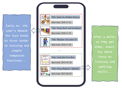
Figure 1. Over time, a noticeable shift in users’ points of interest is observed, reflecting a common characteristic of user interaction behaviors.

Moreover, in comparison to the quadratic computational complexity characteristic of Transformers in the sequence dimension, the Mamba architecture demonstrates the capability to achieve comparable performance with a linear computational complexity. Consequently, recent research efforts have focused on adapting the Mamba architecture for application within the domain of sequential recommendation. The Mamba framework is categorized into two generations: Mamba1 (gu2023mamba) (based on SSM) and Mamba2 (SSD) (based on SSD). We present a comprehensive explanation of SSD and SSM in the section 2.

The Mamba4Rec (mamba4rec) model is the Mamba framework’s first attempt at sequential recommendation tasks, which uses the mamba1 architecture to replace the attention mechanism module without compromising performance and significantly improving computational efficiency. Then, the SSD4Rec (ssd4rec) model was developed based on Mamba2 after Mamba4Rec. Due to the enhanced computational efficiency afforded by the Mamba2 architecture, SSD4Rec achieved superior computational performance in high-dimensional feature spaces. However, it is noteworthy that the Mamba2 architecture exhibits a performance decrement relative to Mamba1 in sequential recommendation tasks. Although SSD4Rec attains performance levels comparable to those of Mamba4Rec in high dimension settings through the implementation of variable sequences and enhancements in bidirectional SSD, since the sequential recommendation task based purely on IDs (identifiers) cannot converge efficiently in high-dimensional spaces, it performs less well than that in low-dimensional environments.

If we solely leverage the advantages of the Mamba2 architecture for high dimension modeling in sequential recommendation tasks, without considering the applicability of high-dimensional processing in pure ID-based sequential recommendation scenarios, the associated computational cost may outweigh its benefits. This is particularly pertinent given that high-dimensional modeling is relatively computationally intensive compared to its low-dimensional counterpart, and purely ID-based sequential recommendation tasks may struggle to converge efficiently in this setting. Thus, addressing the challenge of sustaining performance in low-dimensional feature spaces while leveraging the computational advantages of Mamba2 for modeling sequential recommendation tasks constitutes a critical issue necessitating further investigation.

To address the above issues, this study analyzes the factors contributing to the performance degradation of SSD architecture in comparison to SSM architecture in low-dimensional sequential recommendation tasks. We introduce, for the first time, a time-aware enhancement method tailored for SSD architecture to mitigate this performance loss. This research represents the debut of Mamba architecture in the context of sequential recommendation with respect to time-aware enhancement. It is noteworthy that the time-aware enhancement method proposed in this article preserves the linear computational complexity advantage of the SSD architecture in the sequential dimension. Therefore, in comparison with the SASRec model, which represents the Transformer architecture, and the Mamba4Rec model, which represents the SSM architecture, it retains a significant advantage in terms of model training and inference speed.

We designate our work as TiM4Rec and outline its primary contributions as follows:

• We conduct a pioneering exploration of a time-aware enhancement method tailored for the linear computational complexity of the Mamba architecture in the realm of sequential recommendation.

• Through the introduction of our proposed time-aware enhancement method, we develop the TiM4Rec model, which effectively reduces performance loss in the SSD architecture relative to the SSM architecture in low-dimensional spaces, enhancing its suitability for ID modeling tasks and improving training efficiency.

• Comprehensive experiments across three datasets demonstrate the effectiveness of the TiM4Rec model in low-dimensional spaces, showcasing superior performance compared to SSD4Rec, while maintaining the strengths of the SSD architecture in high-dimensional scenarios.

2. PRELIMINARIES

2.1. Problem Statement

Sequential recommendation methodologies leverage the user’s historical interaction sequences to forecast the subsequent potential interaction item for the user. In particular, tasks that focus solely on predicting the next item in a sequence are referred to as seq2item tasks. This work is also based on the seq2item task for its research. Let $\mathcal{U}=\left\{u_{1},u_{2},\cdots,u_{|\mathcal{U}|}\right\}$ be the set of users and $\mathcal{V}=\left\{v_{1},v_{2},\cdots,v_{|\mathcal{V}|}\right\}$ be the set of items. For any user $u_{k}$, there exists an interaction sequence $\mathcal{S}_{t}^{u_{k}}=\left\{v_{1}^{u_{k}},v_{2}^{u_{k}},\cdots,v_{t}^{u_{k}}\right\}$ at time step $t$, where $v_{i}^{u_{k}}$ represents the i-th item of user $u_{k}$ interaction. Subsequently, by establishing a learnable embedding table $\mathcal{E}=\left\{e_{1},e_{2},\cdots,e_{|\mathcal{V}|}\right\}\in\mathbb{R}^{|\mathcal{V}|\times N}$, the item IDs are converted from a sparse vector representation to a dense vector representation, where $e_{j}$ denotes the potential dense vector representation of the item $v_{j}$. We transform the input sequence $\mathcal{S}_{t}^{u_{k}}$ into the historical interaction vector representation $p^{u_{k}}_{t}$ for user $u_{k}$ through the mapping $\mathcal{F}$. Subsequently, we compute the inner product between $p^{u_{k}}_{t}$ and all item embedding vectors to obtain the predicted score ranking $r_{t}^{u_{k}}$ for the next interaction item.

$$p_{t}^{u_{k}} =\mathcal{F}\left(S_{t}^{u_{k}}\right)$$

$$r_{t}^{u_{k}} =p_{t}^{u_{k}}\cdot\mathcal{E}$$

Finally, we return the IDs of the top $m$ items that the user is likely to interact with, based on the predicted score ranking $r_{t}^{u_{k}}$.

2.2. State Space Models

The State Space Models(SSM) is a sequence modeling framework based on linear ordinary differential equations. It maps the input sequence $x(t)\in\mathbb{R}^{D}$ to the output sequence $y(t)\in\mathbb{R}^{N}$ through the latent state $h(t)\in\mathbb{R}^{N}$:

(1) $$h^{\prime}(t) =\bm{A}h(t)+\bm{B}x(t),$$

$$y(t) =\bm{C}h(t)+\bm{D}x(t),$$

where $\bm{A}\in\mathbb{R}^{N\times N}$ and $\bm{B},\bm{C}\in\mathbb{R}^{N\times D}$ are learnable matrices. To enable SSM to effectively represent discrete data, it is imperative to discretize the data in accordance with the given step size $\Delta$. An effective discretization method for Equation 1 is the Zero Order Hold (ZOH) method (gu2021combining). Assuming the previous time step is $t-1$ and the current time step is $t$, Formula 1 can be solved by using the constant variation method:

$$h(t) =e^{\Delta\bm{A}}h(t-1)+\int_{t-1}^{t}e^{\bm{A}\left(t-\tau\right)}\bm{B}x\left(\tau\right)d\tau$$

$$\approx e^{\Delta\bm{}A}h(t-1)+\int_{t-1}^{t}e^{\bm{A}\left(t-\tau\right)}d\tau\bm{B}x\left(t\right)$$

$$=e^{\Delta\bm{A}}h(t-1)+\left(\Delta\bm{A}\right)^{-1}\left(e^{\Delta\bm{A}}-I\right)\Delta\bm{B}x\left(t\right)$$

We assume $\overline{\bm{A}}=\exp(\Delta\bm{A})$ and $\overline{\bm{B}}=(\Delta\bm{A})^{-1}(\exp(\Delta\bm{A})-\bm{I})\cdot\Delta\bm{B}$, then the following result can be derived:

(2) $$h_{t} =\overline{\bm{A}}h_{t-1}+\overline{\bm{B}}x_{t},$$

$$y_{t} =\bm{C}h_{t}+\bm{D}x_{t},$$

The Structured State Space Model (S4) (gu2021efficiently) is developed from the vanilla SSM. By imposing a structure on the state matrix $\bm{A}\in\mathbb{R}^{D\times N}$ through HiPPO initialization (gu2020hippo), it further enhances the modeling of long-range dependencies.

Based on the foundation established by S4 model, Mamba (gu2023mamba) advances the concept of selectivity by integrating parameter matrices $\Delta\in\mathbb{R}^{T\times D}$, $\bm{B}\in\mathbb{R}^{T\times N}$ and $\bm{C}\in\mathbb{R}^{T\times N}$, which vary over time. Through these methodological advancements, Mamba is capable of selectively transforming the input sequence $\bm{X}\in\mathbb{R}^{T\times D}$ into the output sequence $\bm{Y}\in\mathbb{R}^{T\times D}$ as delineated by the following equation:

$$\bm{Y}_{i}=\sum_{j}\left[\bm{C}_{i}^{\top}\left(\overline{\bm{A}}_{i}\cdot\overline{\bm{B}}_{j}\right)\right]\cdot X_{j}$$

$$\bm{Y}_{i}=\sum_{j}\left\{\bm{C}_{i}^{\top}\left[\left(\prod_{k=1}^{i-j}e^{\Delta_{k}^{\top}\bm{A}}\right)\cdot\left(\Delta_{j}^{\top}\bm{A}\right)^{-1}\left(e^{\Delta_{j}^{\top}\bm{A}}-\bm{I}\right)\cdot\left(\Delta_{j}^{\top}\bm{B}_{j}\right)\right]\right\}\cdot X_{j}$$

Furthermore, the model enhances computational efficiency by employing parallel computation strategies facilitated through the implementation of the Hillis-Steele scan algorithm (hillis1986data). Through the aforementioned enhancements, Mamba demonstrates the capability to attain performance levels that are nearly on par with those of Transformers, while incurring only linear computational complexity with respect to the sequence dimension.

2.3. State Space Duality

The SSM framework, despite employing hardware-aware selective scan algorithms to facilitate parallel computing, encounters limitations in effectively harnessing matrix computation units within the hardware. This inefficacy stems from its non-reliance on matrix operations as a foundational approach. Furthermore, Mamba’s hardware-aware algorithm computational core resides entirely within the GPU’s SRAM, which is typically of limited capacity. This restriction constrains the feature dimensionality in model computations, thereby impeding the ability of the model to operate within higher-dimensional spaces.

From a computational efficiency standpoint, Gu et al. (SSD) innovatively transformed matrix $\bm{A}$ into a scalar value to facilitate SSM matrixization calculation and discovered that this variant of SSM exhibits duality with masked attention mechanisms. To preserve the linear complexity benefit of SSM in the sequence dimension, they leveraged the block properties of semi-separable matrices to implement linear attention computation, culminating in what they termed the Structured State Space Duality.

In essence, SSD, the structure they proposed, initially formulated SSM employing a matrix computation framework:

$$\bm{Y} =SSM(\bm{A},\bm{B},\bm{C})(X)=\bm{M}\bm{X}$$

$$\bm{A}_{m:n}^{\times} \coloneqq\prod_{k=m}^{n}\bm{A}_{k}=\bm{A}_{n}\bm{A}_{n-1}\cdots\bm{A}_{m}$$

(3) $$\bm{M}=\begin{bmatrix}\bm{C}_{0}^{\top}\bm{B}_{0}&&&&\\ \bm{C}_{1}^{\top}\bm{A}_{1}\bm{B}_{0}&\bm{C}_{1}^{\top}\bm{B}_{1}&&&\\ \bm{C}_{2}^{\top}\bm{A}_{2}\bm{A}_{1}\bm{B}_{0}&\bm{C}_{2}^{\top}\bm{A}_{2}\bm{B}_{1}&\bm{C}_{2}^{\top}\bm{B}_{2}&&\\ \vdots&\vdots&\ddots\\ \bm{C}_{i}^{\top}\bm{A}_{1:i}^{\times}\bm{B}_{0}&\bm{C}_{i}^{\top}\bm{A}_{2:i}^{\times}\bm{B}_{1}&\cdots&\bm{C}_{i}^{\top}\bm{B}_{j}\end{bmatrix}$$

In this discussion, we assume the condition where matrices $\bm{A}$ and $\bm{B}$ are not subjected to discretization, allowing us to assert that matrix $\bm{M}_{ij}=\bm{C}_{i}^{\top}\bm{A}_{i-j:i}^{\times}\bm{B}_{j}$. The aforementioned equation delineates the transformation process of the input sequence $\bm{X}\in\mathbb{R}^{T\times D}$ into the output sequence $\bm{Y}\in\mathbb{R}^{T\times D}$ facilitated by the parameter matrices $\bm{A}\in\mathbb{R}^{T\times N}$, $\bm{C}\in\mathbb{R}^{T\times N}$, $\bm{B}\in\mathbb{R}^{T\times N}$ and $\bm{M}\in\mathbb{R}^{T\times T}$. The inefficiency of SSM in executing matrix operations stems from the computational demands constrained by the recursive computational load of matrix $\bm{A}_{m:n}^{\times}$ in a temporal sequence. Consequently, by simplifying matrix $\bm{A}_{m:n}^{\times}$ to a scalar and leveraging the properties of semi-separable matrices, we can significantly enhance the efficiency of matrix computations involving matrix $\bm{M}$. Under the assumption that $\bm{A}=[1,a_{1},\dots,a_{t-1}]\in\mathbb{R}^{T}$, SSD facilitates the computation of matrix $\bm{M}$ by introducing a 1-Semi Separable (1-SS) matrix $\bm{L}\in\mathbb{R}^{T\times T}$ defined as follows:

(4) $$\bm{L}=\begin{bmatrix}1\\ a_{1}&1\\ a_{2}a_{1}&a_{2}&1\\ \vdots&\vdots&\ddots&\ddots\\ a_{t-1}\ldots a_{1}&a_{t-1}\ldots a_{2}&\cdots&a_{t-1}&1\end{bmatrix}$$

$$\bm{M}_{i+1,j+1}=\bm{C}_{i}^{\top}\bm{A}_{i:j}\bm{B}_{j}\coloneqq\bm{C}_{i}^{\top}a_{i}\ldots a_{j+1}\bm{B}_{j}$$

Thus, we can equivalently derive the following equation:

$$\bm{M}=\bm{L}\circ\bm{C}\bm{B}^{\top}$$

$$\bm{M}=\begin{bmatrix}\bm{C}_{0}^{\top}\bm{A}_{0:0}\bm{B}_{0}&&&&\\ \bm{C}_{1}^{\top}\bm{A}_{1:1}\bm{B}_{0}&\bm{C}_{1}^{\top}\bm{A}_{1:1}\bm{B}_{1}&&&\\ \bm{C}_{2}^{\top}\bm{A}_{2:1}\bm{B}_{0}&\bm{C}_{2}^{\top}\bm{A}_{2:1}\bm{B}_{1}&\bm{C}_{2}^{\top}\bm{A}_{2:2}\bm{B}_{2}&&\\ \vdots&\vdots&\ddots\\ \bm{C}_{i}^{\top}\bm{A}_{i:1}\bm{B}_{0}&\bm{C}_{i}^{\top}\bm{A}_{i:2}\bm{B}_{1}&\cdots&\bm{C}_{i}^{\top}\bm{A}_{i:i}\bm{B}_{i}\end{bmatrix}$$

By considering matrix $\bm{C}$ as matrix $\bm{Q}$, matrix $\bm{B}$ as matrix $\bm{K}$ and matrix $\bm{X}$ as matrix $\bm{V}$ within the framework of the attention mechanism and excluding the Softmax computation, a profound conclusion is reached:

$$\bm{Y}=\bm{L}\circ\bm{C}\bm{B}^{\top}\bm{X}=\bm{L}\circ\bm{Q}\bm{K}^{\top}\bm{V}$$

This concept is referred to as Duality in the SSD framework. By referring to the tensor contraction order in the calculation of linear attention (LinearAttention)—specifically using the associative property of matrix multiplication where $K^{T}V$ is computed first and subsequently left-multiplied by $Q$—the computational complexity is reduced from quadratic to linear in the sequence dimension without considering causal masks, a property that SSD also achieves.

$$\bm{Y}=\left(\bm{Q}\bm{K}^{T}\right)\bm{V}\quad\Rightarrow\quad\bm{Y}=\bm{Q}\left(\bm{K}^{T}\bm{V}\right)$$

$$\bm{Y}=\left(\bm{C}\bm{B}^{T}\right)\bm{X}\quad\Rightarrow\quad\bm{Y}=\bm{C}\left(\bm{B}^{T}\bm{X}\right)$$

To integrate causal masking without compromising linear computational complexity, the block properties of the 1-SS matrix $\bm{L}$ can be leveraged in conjunction with segment accumulation. This approach facilitates the implementation of causal linear attention, referred to as Structured Masked Attention (SMA) (SSD) in SSD. Since the SSD architecture is derived from the Mamba model, models based on the SSD architecture are referred to as Mamba2. Although SSD offers significant advantages in terms of computational load—particularly in tasks with high feature dimensions—the performance of SSD in sequential recommendation tasks is inferior compared to Mamba1. We provide a detailed analysis of this issue in the following sections.

3. THE PROPOSED METHOD

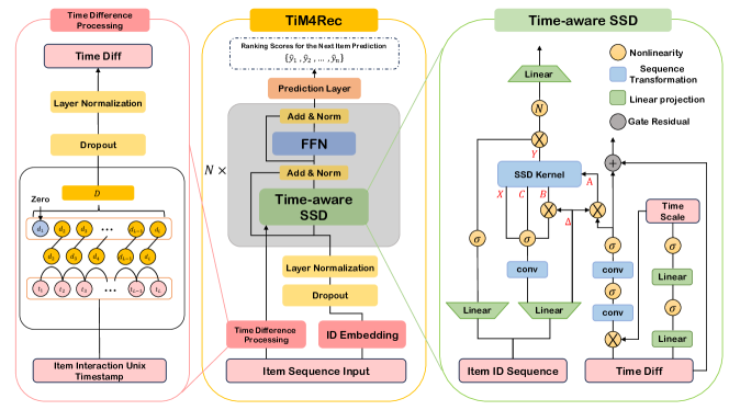
Figure 2. The overall framework of TiM4Rec, which is based on time-aware enhancement, enhances the performance of the SSD architecture in the domain of sequential recommendation by effectively processing the time differences in interactions between items.

In this section, we provide a detailed introduction to our proposed framework, TiM4Rec. After presenting an overview of the overall structure of TiM4Rec, we explore the reasons behind the performance degradation of SSD compared to SSM in low-dimensional scenarios within sequential recommendation tasks. Subsequently, we introduce how our time-aware enhancement method compensates for this loss while maintaining linear computational complexity.

3.1. Overview of TiM4Rec

As shown in Figure 2, the overall logic of TiM4Rec adheres to the description in section 2.1, However, an additional user interaction unix timestamp sequence $\mathcal{T}^{u_{k}}=\left\{t_{1},t_{2},\cdots,t_{L}\right\}\in\mathbb{R}^{L}$ is incorporated into the input data, with $\mathcal{T}^{u_{k}}$ corresponding one to one with the user interation sequence $\mathcal{S}^{u_{k}}$, where $L$ representing interaction sequence length. The sequence $\mathcal{S}^{u_{k}}$ can be transformed into an input sequence $\bm{X}\in\mathbb{R}^{T\times D}$ composed of dense vectors by the embedding table $\mathcal{E}$. Subsequently, a displacement subtraction is performed on sequence $\mathcal{T}^{u_{k}}$, and a zero is appended to the begining to generate the intearaction time difference sequence $\mathcal{D}^{u_{k}}=\left\{d_{1},d_{2},\cdots,d_{L}\right\}\in\mathbb{R}^{L}$, which be used in later stages. The Time-aware SSD Block enhances the model’s ability to capture potential user interests by integrating sequence $\mathcal{D}^{u_{k}}$ into a discretized SSD kernel. For the sake of convenience in the subsequent discussion, the superscript $u_{k}$ be omitted.

3.2. Time Difference Processing

As mentioned above, for the input interaction timestamp sequence $\mathcal{T}$, we transform it into an interaction time difference sequence $\mathcal{D}$ using the following method:

(5) $$\mathcal{D}_{i}=\begin{cases}0,\quad&i=1\\ \mathcal{T}_{i}-\mathcal{T}_{i-1},\quad&i\in\left[2,L\right]\end{cases}$$

Subsequently, we apply dropout (srivastava2014dropout) and layer normalization (ba2016layer) to sequence $\mathcal{D}$ in order to eliminate data noise and optimize the data distribution for subsequent analysis.

3.3. Analyzing the Mask Matrix in SSD

As discussed in section 2.3, the critical advancement from SSM to SSD resides in the scalarization of the transition matrix $\bm{A}$. When considering this modification from an attention perspective, the central aspect involves the alterations in the mask matric $\bm{L}$. Although the recursive operational constraints of matrix $\bm{A}$ in SSM prevent the direct and precise formulation of the mask matrix within eq. 3, it remains feasible to examine an equivalent expression for the final mask matrix:

$$\bm{L}_{\text{SSM}}=\begin{bmatrix}I\\ \bm{A}_{1}&I\\ \bm{A}_{2}\bm{A}_{1}&\bm{A}_{2}&I\\ \vdots&\vdots&\ddots&\ddots\\ \bm{A}_{1:i}^{\times}&\bm{A}_{2:i}^{\times}&\cdots&\bm{A}_{i-1:i}^{\times}&I\end{bmatrix}$$

As illustrated in figure 3, in contrast to the mask matrix of SSD presented in eq. 4, the fundamental change in the mask matrix $L_{\text{SSM}}$ is that its mask coefficients are applied in a point-to-point manner on the individual item $\bm{E}_{i}=\left[e_{1},e_{2},\cdots,e_{n}\right]\in\mathbb{R}^{N}$ (The $\bm{A}$ matrix follows its definitions in SSM and SSD, respectively.):

$$\text{SSM:}\quad\hat{\bm{E}}_{i}=\bm{A}^{\times}_{p:q}\cdot\bm{E}_{i},\quad\bm{A}^{\times}_{p:q}\in\mathbb{R}^{N}$$

$$\text{SSD:}\quad\hat{\bm{E}}_{i}=\bm{A}_{p:q}\cdot\bm{E}_{i},\quad\bm{A}_{p:q}\in\mathbb{R}^{1}$$

In instances where the $\bm{E}$ is in low dimension, its relative contribution to information is diminished, necessitating a more refined filtering of $\bm{E}$ by the mask matrix. Consequently, the point-to-point masking employed in SSM demonstrates superior performance in low-dimensional contexts. Notably, from the perspective of masking strategies, SSD exhibits a greater inclination towards the Transformer architecture than SSM.

$$\bm{L}_{MSA}=\begin{bmatrix}1\\ 1&1\\ 1&1&1\\ \vdots&\vdots&\ddots&\ddots\\ 1&1&\cdots&1&1\end{bmatrix},$$

MSA stands for Vanilla Mask Self Attention Mechanism

However, owing to the semi-separable matrix structure inherent in the mask matrix of SSD, there is a pronounced attenuation effect on the interaction items that appear earlier in the sequence. This feature aligns SSD more closely with the actual user interaction patterns observed in real-world recommendation systems. Consequently, it is anticipated that, under equivalent conditions in low-dimensional settings, the SSM architecture exhibit superior performance in the realm of sequential recommendation, followed by SSD, with the Transformer architecture trailing behind. This hypothesis is further corroborated by the findings presented in our subsequent experimental section.

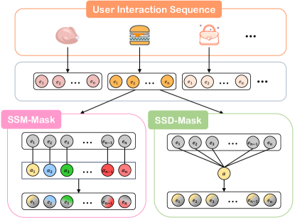
Figure 3. The distinction in mask formulation between SSD and SSM is noteworthy. For an individual item, SSM can be viewed as an equivalent point-to-point mask, whereas SSD resembles the global mask utilized in Transformer architectures.

Observing the differences between the equivalent mask matrices of SSD and SSM, it can be seen that the core of their mask matrices is recursively generated based on the state transition matrix $\bm{A}$. As described in section 2.3, the only difference is that SSD achieves more efficient matrix multiplication calculations by scalar quantization of matrix $\bm{A}$. Therefore, addressing the loss of the mask matrix caused by the scalar quantization of matrix $\bm{A}$ while maintaining the efficient matrix multiplication calculation of SSD has become the key to improvement.

3.4. Time-aware Mask Matrix

Let’s reconsider how the time difference matrix should be expressed in the context of attention mechanisms. The method proposed by TiSASRec (TiSASRec) is centered around acquiring the time position encoding for each item in the interaction sequence through interaction timestamps, ultimately leading to the generation of the corresponding attention bias matrix based on these encodings. Given that the Mamba architecture does not depend on positional encoding—as substantiated by the findings in Mamba4Rec (mamba4rec) and SSD4Rec (ssd4rec)—it is essential to directly explore the equivalent representation of the TiSASRec approach. Specifically, we should investigate how the resulting attention bias matrix encapsulates the temporal differences in product interactions.

For a sequence of interactive timestamps $\mathcal{T}$, we can derive the relative time difference matrix $\hat{\mathcal{D}}$ between each product through the following transformation:

(6) $$\hat{\mathcal{D}}=\begin{bmatrix}\hat{d}_{11}\\ \mathbf{\underline{\hat{d}_{21}}}&\hat{d}_{22}\\ \hat{d}_{31}&\mathbf{\underline{\hat{d}_{32}}}&\hat{d}_{33}\\ \vdots&\vdots&\ddots&\ddots\\ \hat{d}_{L1}&\hat{d}_{L2}&\cdots&\mathbf{\underline{\hat{d}_{LL-1}}}&\hat{d}_{LL}\end{bmatrix},\quad\hat{d}_{mn}=t_{m}-t_{n}$$

Directly applying matrix $\hat{\mathcal{D}}$ to the mask matrix $\bm{L}$ (as described in eq. 4) compromises the semi-separable matrix property of $\bm{L}$. This compromise prevents us from leveraging the efficient matrix computation techniques offered by the SSD architecture, consequently resulting in a return to quadratic computational complexity. Therefore, it is imperative to modify the insertion method of matrix $\hat{\mathcal{D}}$.

When we construct a new matrix $\mathcal{D}$ by selecting only the values of the underlined elements in matrix $\hat{\mathcal{D}}$, we effectively adopt the form described in eq. 5. This approach allows us to integrate matrix $\mathcal{D}$ into the mask matrix $\bm{L}$ with linear complexity. Initially, we apply matrix $\mathcal{D}$ to the scalarization matrix $\bm{A}$, which results in the corresponding positions in the mask matrix $\bm{L}$ containing the relevant time difference information (Due to the presence of layer normalization, the actual value of $d_{1}$ will be non-zero.):

$$\hat{\bm{A}}_{i}=\hat{a}_{i}=\mathcal{D}_{i}\cdot\bm{A}_{i}=\hat{d}_{ii-1}\cdot a_{i}=d_{i}\cdot a_{i}$$

$$\hat{\bm{A}}_{m:n}\coloneqq\hat{a}_{n}\hat{a}_{n-1}\cdots\hat{a}_{m}=a_{n}d_{n}\cdot a_{n-1}d_{n-1}\cdots a_{m}d_{m}$$

(7) $$\bm{L}=\begin{bmatrix}1\\ \hat{a}_{1}&1\\ \hat{a}_{2}\hat{a}_{1}&\hat{a}_{2}&1\\ \vdots&\vdots&\ddots&\ddots\\ \hat{a}_{t-1}\ldots\hat{a}_{1}&\hat{a}_{t-1}\ldots\hat{a}_{2}&\cdots&\hat{a}_{t-1}&1\end{bmatrix}$$

This can be regarded as an equivalent approximation of $d_{ij}$ as follows:

$$\hat{d}_{ij}\approx\hat{d}_{ii-1}\hat{d}_{i-1i-2}\cdots\hat{d}_{j+1j}=d_{i}d_{i-1}\cdots d_{j}$$

In the context of SSD kernel computations, multiplication is effectively converted into accumulation operations via the logarithm function. This transformation offers advantageous support for the aforementioned approximation of $\hat{d}_{ij}$.

$$\log\left(d_{i}d_{i-1}\cdots d_{j}\right)=\log\left(d_{i}\right)+\log\left(d_{i-1}\right)+\cdots+\log\left(d_{j}\right)$$

Through the approximation method mentioned above, we accomplish the time-aware enhancement of the SSD architecture. This is achieved without disrupting the semi-separable property of the mask matrix $\bm{L}$.

3.5. Time-aware SSD Block

Despite providing a detailed derivation of the SSD in Section 2.3, the actual code implementation of the SSD kernel retains the discretization process. Therefore, further analysis is required. Notably, in Section 2.2, we derive the discretization for the SSM, but it is important to highlight that the actual computational process is approximated in both SSM and SSD implementations. Specifically, for matrix $\overline{\bm{A}}$, the implementation approximates the exponential operation by directly computing $\overline{\bm{A}}\approx\Delta\bm{A}$. Meanwhile, for matrix $\overline{\bm{B}}$, given the Maclaurin series expansion of $e^{x}$ as $1+x+\frac{x^{2}}{2}+\cdots$, the following approximation can be made:

$$\overline{\bm{B}} \approx\left(\Delta\bm{A}\right)^{-1}\left(\bm{I}+\Delta\bm{A}-\bm{I}\right)\cdot\Delta\bm{B}$$

$$=\left(\Delta\bm{A}\right)^{-1}\Delta\bm{A}\cdot\Delta\bm{B}$$

$$=\Delta\bm{B}$$

In this approximation, we establish the following definitions: the state transition coefficient $\bm{A}\in\mathbb{R}^{1}$. By inputting $\bm{X}\in\mathbb{R}^{T\times D}$, we derive matrices $\bm{B}\in\mathbb{R}^{T\times N}$ and $\bm{C}\in\mathbb{R}^{T\times N}$, along with the discretization parameter $\Delta\in\mathbb{R}^{T}$:

$$\bm{X},\bm{B},\bm{C},\Delta=\bm{X}W+b$$

Where the weight matrix $W\in\mathbb{R}^{D\times(D+2N+1)}$ and the bias matrix $b\in\mathbb{R}^{D+2N+1}$. Subsequently, a causal convolution transformation is applied to the matrices $\bm{X}$, $\bm{B}$ and $\bm{C}$:

$$\bm{X}_{t},\bm{B}_{t},\bm{C}_{t} =\sigma\left[(\bm{X}_{t},\bm{B}_{t},\bm{C}_{t})^{\top}*\omega\right]$$

$$\text{where}\quad\mathcal{Q}_{t}=\mathcal{P}_{t}*\omega \coloneqq\sum_{m=0}^{K-1}\mathcal{P}_{\max\left(t-m,0\right)}\cdot\omega_{m}$$

Where the $\omega\in\mathbb{R}^{K}$ is convolution kernel and the $\sigma$ represents non-linear activation functions.

Before proceeding with the derivation, it is prudent to examine how the time difference vector $\mathcal{D}$ is integrated into the discretized SSD. Regarding the time difference matrix $\mathcal{D}$, we note that the implicit interest conveyed by the same interaction time difference can vary across different user interaction contexts. Therefore, we initially apply a time-varying transformation to the time difference matrix using the following transformation:

$$\alpha^{\mathcal{D}}=\sigma\left[\sigma\left(\mathcal{D}W_{1}^{\mathcal{D}}+b_{1}^{\mathcal{D}}\right)W_{2}^{\mathcal{D}}+b_{2}^{\mathcal{D}}\right]$$

$$\mathcal{D}=\alpha^{\mathcal{D}}\cdot\mathcal{D}$$

Where the weight matrix $W_{1}^{\mathcal{D}},W_{2}^{\mathcal{D}}\in\mathbb{R}^{T\times T}$ and the bias matrix $b_{1}^{\mathcal{D}},b_{2}^{\mathcal{D}}\in\mathbb{R}^{T}$. Considering the convergence of interaction time differences within a short time frame, we apply causal convolution to the time difference matrix $\mathcal{D}$ to enhance the implicit features of user interest points.

$$\mathcal{D}_{t}=\sigma\left(\mathcal{D}_{t}*\omega^{\mathcal{D}}\right)\coloneqq\sigma\left(\sum_{m=0}^{K-1}\mathcal{D}_{\max\left(t-m,0\right)}\cdot\omega^{\mathcal{D}}_{m}\right)$$

Next, we integrate the enhanced time difference matrix $\mathcal{D}$ with the discrete parameter $\Delta$, and obtain matrices $\overline{\bm{A}}$ and $\overline{\bm{B}}$ through the following transformation:

$$\hat{\Delta}=\Delta\cdot\mathcal{D},\quad\overline{\bm{A}}=\hat{\bm{A}}=\hat{\Delta}\cdot\bm{A},\quad\overline{\bm{B}}=\hat{\Delta}\cdot\bm{B}$$

Finally, the following equation can be derived to map the input $\bm{X}$ to the output $\bm{Y}\in\mathbb{R}^{T\times D}$($\bm{L}$ refers to eq. 7.):

$$\bm{Y}=\bm{L}\circ\bm{C}\overline{\bm{B}}^{\top}\bm{X}=\bm{L}\circ\bm{C}\bm{B}^{\top}\left(\hat{\Delta}^{\top}\bm{X}\right)$$

Due to the preservation of the semi-separable matrix property of $\bm{L}$, the matrix computation acceleration method discussed in Section 2.3 remains applicable.

To extract deeper user interest features, multiple layers of Time-aware SSD blocks are stacked. Consequently, after the Time-aware SSD, the features are transformed by adding a Feed Forward Network layer to adapt to the next semantic space. It is noteworthy that to adapt the time difference vector $\mathcal{D}$ to the feature semantic space of the next layer, gate residual (he2016deep) processing is applied to the input time difference vector $\mathcal{D}$ for the subsequent layer.

3.6. Prediction Layer

By utilizing the Time-aware SSD Block, input $\bm{X}$ can be transformed into a user interest feature sequence $\bm{P}\in\mathbb{R}^{L\times D}$. The last element $p_{t}$ of the feature sequence $\bm{P}$ is then extracted as the interest feature corresponding to the current user interaction sequence.

$$\hat{\mathcal{Y}}=Softmax\left(p_{t}\cdot\mathcal{E}\right)$$

As stated in Section 2.1, the predicted scores $\hat{\mathcal{Y}}\in\mathbb{R}^{|\mathcal{V}|}$ for all items are obtained by calculating the inner product of $p_{t}$ and the embedding table of all items. However, a notable difference is that the actual score calculation incorporates the Softmax function, even though the Softmax operation does not influence the ranking of the scores.

3.7. Complexity Analysis

Models based on the Vanilla Transformer, such as SASRec, require a total of $O(L^{2}N)$ floating-point operations (FLOPs). In contrast, thanks to the computational improvements provided by Mamba, models based on SSM and SSD, such as Mamba4Rec and SSD4Rec, only require $O(LN^{2})$ FLOPs. In practical application scenarios of sequential recommendation, including news and product recommendations, it is often the case that $L\gg N$. Thus, sequential recommendation models based on Mamba demonstrate superior advantages. TiSASRec enhances its performance by integrating time-aware capabilities via time difference encoding. Despite the theoretical FLOPS remaining in the order of $O(L^{2}N)$, the practical computational and memory demands exceed those of SASRec by more than four times. This substantial increase is attributed to the inherent computational constraints associated with time difference encoding. Consequently, while TiSASRec demonstrates improved time sensitivity, it necessitates a significantly higher computational overhead and memory allocation compared to SASRec, posing potential challenges in scalability and efficiency. In contrast, TiM4Rec preserves the benefits of the SSD architecture by employing a time difference mask matrix characterized by linear computational complexity. This approach maintains the computational efficiency, demanding only $O(LN^{2})$ FLOPs, and incurs only a modest increase in additional computational overhead. Notably, the generation of the time-aware mask matrix in TiM4Rec is solely based on scalar computations. This characteristic ensures that the additional computational complexity does not escalate in high-dimensional modeling scenarios, thereby preserving the superior matrix operation efficiency inherent to the SSD4Rec architecture.

Table 1. Comparison of computational complexity between representative sequential recommendation methods, where ”M.M.” refers to ”Matrix Multiplication”.

	Architecture	FLOPs	Memory	M.M.
SASRec	Attention	$L^{2}N$	$L^{2}N$	✓
Mamba4Rec	SSM	$LN^{2}$	$LN^{2}$
SSD4Rec	SSD	$LN^{2}$	$LN$	✓
TiSASRec	Attention	$L^{2}N$	$L^{2}N$	✓
TiM4Rec	SSD	$LN^{2}$	$LN$	✓

4. Experiments

Table 2. Sequential recommendation performance on the ML1M, Beauty, and KuaiRand datasets. Here, R@k refers to Recall@K, N@K denotes NDCG@K, and M@K represents MRR@K. The best and second-best results are indicated in bold and underlined, respectively. ”Improv.” signifies the performance improvement of TiM4Rec compared to the second-best results. The asterisk in SSD4Rec* denotes that this is our own replicated version.

Model Type & Model $\rightarrow$			CNN	RNN	Transformer			SSM	SSD		Improv.
Dataset	Metric		Caser	GRU4Rec	SASRec	BERT4Rec	TiSASRec	Mamba4Rec	SSD4Rec*	TiM4Rec
MovieLens-1M	R@10		0.2156	0.2985	0.3060	0.2800	0.3147	0.3253	0.3199	0.3310	1.75%
	R@20		0.3083	0.3937	0.4050	0.3853	0.4250	0.4354	0.4240	0.4338	-0.30%
	R@50		0.4515	0.5397	0.5455	0.5377	0.5608	0.5707	0.5649	0.5770	1.10%
	N@10		0.1157	0.1700	0.1754	0.1584	0.1834	0.1891	0.1841	0.1932	2.17%
	N@20		0.1391	0.1941	0.2005	0.1852	0.2106	0.2169	0.2104	0.2194	1.15%
	N@50		0.1675	0.2232	0.2285	0.2154	0.2376	0.2436	0.2384	0.2477	1.68%
	M@10		0.0853	0.1307	0.1357	0.1214	0.1424	0.1474	0.1425	0.1512	2.58%
	M@20		0.0917	0.1373	0.1425	0.1288	0.1498	0.1551	0.1498	0.1584	2.13%
	M@50		0.0963	0.1420	0.1471	0.1337	0.1542	0.1593	0.1542	0.1629	2.26%
Amazon Beauty	R@10		0.0402	0.0563	0.0851	0.0352	0.0802	0.0838	0.0806	0.0854	0.35%
	R@20		0.0618	0.0856	0.1194	0.0563	0.1147	0.1185	0.1146	0.1204	0.84%
	R@50		0.1090	0.1376	0.1759	0.0999	0.1734	0.1802	0.1710	0.1800	-0.11%
	N@10		0.0199	0.0297	0.0425	0.0172	0.0405	0.0435	0.0423	0.0446	2.53%
	N@20		0.0253	0.0371	0.0511	0.0225	0.0491	0.0522	0.0509	0.0533	2.11%
	N@50		0.0346	0.0473	0.0623	0.0311	0.0605	0.0644	0.0620	0.0651	1.09%
	M@10		0.0138	0.0217	0.0294	0.0117	0.0282	0.0311	0.0306	0.0321	3.22%
	M@20		0.0153	0.0237	0.0317	0.0132	0.0306	0.0335	0.0329	0.0345	2.99%
	M@50		0.0167	0.0253	0.0335	0.0145	0.0325	0.0354	0.0347	0.0363	2.54%
Kuai Rand	R@10		0.0801	0.1020	0.1055	0.0938	0.1057	0.1094	0.1055	0.1109	1.37%
	R@20		0.1344	0.1659	0.1704	0.1537	0.1710	0.1768	0.1717	0.1774	0.34%
	R@50		0.2561	0.3017	0.3074	0.2873	0.3060	0.3154	0.3088	0.3202	1.52%
	N@10		0.0395	0.0564	0.0584	0.0510	0.0590	0.0608	0.5880	0.0611	0.49%
	N@20		0.0531	0.0724	0.0747	0.0660	0.0753	0.0777	0.0754	0.0779	0.26%
	N@50		0.0770	0.0911	0.1016	0.0923	0.1019	0.1050	0.1024	0.1060	0.95%
	M@10		0.0273	0.0428	0.0443	0.0382	0.0450	0.0461	0.0449	0.0463	0.43%
	M@20		0.0310	0.0471	0.0487	0.0422	0.0494	0.0508	0.0494	0.0508	-
	M@50		0.0347	0.0513	0.0529	0.0464	0.0536	0.0552	0.0536	0.0552	-

4.1. Experimental Setup

4.1.1. Datasets

The performance of our proposed model is evaluated through experiments conducted on three publicly available datasets, which have previously been utilized as evaluation benchmarks in several classical sequential recommendation models.

• MovieLens-1M (harper2015movielens): A dataset containing approximately 1 million user ratings for movies, collected from the MovieLens platform.

• Amazon-Beauty (mcauley2015image): The user review dataset collected in the beauty category on the Amazon platform was compiled up to the year 2014.

• Kuai Rand (kuairand): Acquired from the recommendation logs of the application Kuaishou, the dataset includes millions of interactions involving items that were randomly displayed.

For each user, we sort their interaction records according to the timestamps, thereby generating an interaction sequence for each individual. And then retain only those users and items that are associated with a minimum of five interaction records, in accordance with the methodology established in prior research (kang2018self). The statistics of these datasets are shown in Table 3.

4.1.2. Baseline

To demonstrate the superiority of our proposed method, we select a set of representative sequential recommendation models to serve as baselines. Notably, even though SSD4Rec (ssd4rec) has not been released as open-source, we implemented a variant termed SSD4Rec*, adhering to the traditional sequential recommendation framework to validate the efficacy of our time-aware approach. This implementation is strictly based on the SSD architecture and does not incorporate features such as variable-length sequences and bidirectional SSD methods proposed in SSD4Rec. The exclusion of these features is intentional, as they are generally regarded as universal enhancement techniques, particularly in the context of handling variable-length sequences.

• Caser (tang2018personalized): A classical sequential recommendation model based on CNN.

• GRU4Rec (GRU4Rec): A RNN-based method constructed by Gated Recurrent Units (GRU).

• SASRec (kang2018self): The first exploration model of applying Transformer in the field of sequential recommendation.

• BERT4Rec (sun2019bert4rec): A bidirectional attention sequential recommendation model following the BERT (bert) model paradigm.

• TiSASRec (TiSASRec): A time-aware enhanced sequential recommendation model based on SASRec: Considered as paradigm in time-aware sequential recommendation research.

• Mamba4Rec (mamba4rec): A pioneering model that explores the application of the Mamba architecture in the domain of sequential recommendation.

• SSD4Rec (ssd4rec): The pioneering sequential recommendation model leveraging the SSD architecture, exploits its inherent advantages over the SSM architecture for high-dimensional modeling, and integrates variable-length sequence training techniques to enhance model performance.

4.1.3. Evaluation Metrics

We employ well-established recommendation performance metrics including Hit Ratio (HR@K), Normalized Discounted Cumulative Gain (NDCG@K), and Mean Reciprocal Rank (MRR@K) as the criteria for experimental assessment. In calculating these metrics, it is necessary to extract the top K scores from the model’s final predicted ranking. We choose K values of 10, 20, and 50 to encompass short, medium, and long prediction lengths.

Table 3. Statistics of the experimented datasets.

Dataset	ML-1M	Beauty	KuaiRand
#Users	6,040	22,363	23,951
#Items	3,416	12,101	7,111
#Interactions	999,611	198,502	1,134,420
Avg.Length	165.5	8.9	47.4
Max.Length	2,314	389	809
Sparsity	95.15%	99.93%	99.33%

4.1.4. Implementation Details

Our experimental procedures adhere to the paradigm requirements set by the PyTorch (paszke2019pytorch) and RecBole (recbole[1.2.0]). All models in the experiment are implemented with a model dimension of 64, which is the conventional choice for sequential recommendation models based on pure ID modeling. For models based on the Mamba architecture, such as Mamba4Rec, SSD4Rec* and TiM4Rec, the SSM state factor was consistently set to 32, the kernel size for 1D causal convolution is 4, and the block expansion factor for linear projections is 2. It is notable that the 1D causal convolutional layer within the Mamba architecture constrains the multi-head parameter to multiples of 8. However, in the context of sequential recommendation, this parameter typically holds values of 2 or 4. Consequently, we modify the 1D causal convolutional layer to accommodate the specific modeling tasks of sequential recommendation, ultimately standardizing it to a value of 4. The backbone layers across all models are consistently configured to a depth of 2. To address the sparsity of the Amazon datasets, a dropout rate of 0.4 is used, compared to 0.2 for MovieLens-1M and KuaiRand. The Adam optimizer (kingma2014adam) is used uniformly with a learning rate set to 0.01. A batch size of 2048 is employed for training, and the validated batch size is 4096. The maximum sequence length is set proportionally to the mean number of actions per user: 200 for MovieLens1M and 50 for Amazon-Beauty and KuaiRand datasets. We adhere to the optimal parameter configurations specific to each baseline, ensuring that the core parameters remain consistent across all models, and make adjustments to maximize performance to the extent feasible.

4.2. Performance Comparison

We initially conduct a comparative analysis of the recommendation performance between our proposed model and several baseline models across three benchmark datasets. The results of this comparison are presented in Table 2. Through a detailed examination of the experimental outcomes, we are able to derive the following conclusions:

• In low-dimensional settings, the SSD architecture experiences a considerable decline in recommendation performance compared to the SSM architecture. However, when compared with models founded on Transformer architectures, it exhibits enhanced performance. This observation aligns with our theoretical analysis presented in Section 3.3.

• TiM4Rec exhibits a significant performance enhancement when compared to SSD4Rec*, which is modeled on a purely SSD-based architecture, thereby confirming the efficacy of the Time-aware SSD Block. Furthermore, TiM4Rec demonstrates a slight performance advantage over Mamba4Rec. This observation underscores the effectiveness of leveraging temporal differences in user interactions to capture shifts in user interests, effectively mitigating the performance decline observed when transitioning from the SSM architecture to the SSD architecture.

4.3. Dimension comparison

To assess the suitability of modeling pure ID sequence recommendation tasks in lower dimensions, we compare the experimental results presented in the SSD4Rec paper at 256 dimensions. These results are shown in Table 4. Our research findings clearly demonstrate that the Mamba4Rec model tends to exhibit superior performance in 64-dimensional space. Additionally, the SSD4Rec* model that we replicate, which does not utilize variable-length sequences or bidirectional SSDs, showed only a slight decline in performance at 64 dimensions compared to the results presented in the original SSD4Rec paper at 256 dimensions. Notably, the performance of SSD4Rec at 256 dimensions is even inferior to that Mamba4Rec at 64 dimensions. These findings provide robust evidence that pure ID sequence recommendation tasks are more effectively modeled in lower-dimensional spaces. Moreover, the computational overhead associated with 256 dimensions is substantially higher, underscoring the advantages of utilizing our model. In addtional, a key advantage of the SSD architecture over the SSM architecture is its superior capability in high-dimensional modeling. To validate this advantage, we conduct a comparative analysis of the performance of our proposed method, TiM4Rec, at a dimensionality of 256. The results confirm that TiM4Rec effectively preserves the benefits of the SSD architecture even in high-dimensional settings.

Table 4. The performance of sequential recommendation models based on SSM and SSD is compared on the ML1M dataset in 64 and 256 dimensions. The definitions are aligned with the provisions of Table 2.

Dimension $\rightarrow$		64D			256D
Metric		Mamba4Rec	SSD4Rec*	TiM4Rec	Mamba4Rec	SSD4Rec	TiM4Rec
R@10		0.3253	0.3199	0.3310	0.3124	0.3152	0.3270
R@20		0.4354	0.4240	0.4338	0.4103	0.4194	0.4272
N@10		0.1891	0.1841	0.1932	0.1847	0.1889	0.1938
N@20		0.2169	0.2104	0.2194	0.2094	0.2145	0.2191
M@10		0.1474	0.1425	0.1512	0.1456	0.1495	0.1529
M@20		0.1551	0.1498	0.1584	0.1523	0.1565	0.1598

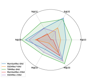
Figure 4. Regarding the performance radar chart of Table 4

4.4. Efficiency Analysis

In this section, we verify whether TiM4Rec can retain the inherent advantages of SSD architecture during model training and inference. Table 5 presents the training and inference times for representative models built on Transformer and Mamba architectures, all executed on a single NVIDIA RTX 3090 GPU.

Observing the experimental results, we can draw the following conclusions:

• In both high-dimensional and low-dimensional spaces, TiM4Rec effectively preserves the inherent computational efficiency of the SSD architecture, necessitating only a minimal additional computational load when compared to SSD4Rec*, which is exclusively based on the SSD architecture. Notably, when compared with SASRec and Mamba4Rec, TiM4Rec achieves substantial enhancements in computational efficiency, attributed to leveraging the high-efficiency computing capabilities of the SSD architecture. This demonstrates TiM4Rec’s ability to significantly optimize computational processes while minimizing overhead, thereby underscoring its advantage in scenarios demanding efficient and scalable solutions.

• Although TiSASRec maintains the computational complexity akin to that of SASRec, its time-aware methodology introduces notable inefficiencies, leading to a substantial escalation in actual computational load. By contrast, TiM4Rec demonstrates remarkable efficiency by necessitating only minimal additional computational resources across both high-dimensional and low-dimensional domains. The experimental results robustly validate the efficacy of the proposed time-aware enhancement method, which maintains linear computational complexity, underscoring its potential as an effective solution for efficient sequential recommendation systems.

Table 5. Comparison of training and inference times across various models using the ML-1M dataset. All models have a dimensionality of 64, except those with 256d suffix.

Model	Architecture	Training Time	Inference Time
SASRec	Attention	207.42s	0.81s
TiSASRec	Attention	1149.57s	1.89s
Mamba4Rec	SSM	111.76s	0.26s
SSD4Rec*	SSD	74.43s	0.18s
TiM4Rec	SSD	83.57s	0.21s
SSD4Rec*-256d	SSD	338.23s	0.64s
TiM4Rec-256d	SSD	342.38s	0.64s

It is noteworthy that although we only compare the computational efficiency of our own replicated version of SSD4Rec*, the actual computational efficiency of SSD4Rec* surpasses that of SSD4Rec because SSD4Rec* eliminates the bidirectional SSD processing and the variable length sequence methods originally proposed in SSD4Rec, which come with additional overhead.

4.5. Ablation experiment

To validate the efficacy of our proposed time-aware algorithm along with other critical design elements, we perform a series of ablation experiments using the ML-1M dataset. The procedure for the systematic elimination of each component is detailed as follows:

• w/o Time : Remove the proposed time-aware algorithm from the SSD module, rendering the model equivalent to our replication of the SSD4Rec* model mentioned earlier.

• w/o FFN : To assess the necessity of the FFN layer’s nonlinear transformation ability in extracting sequential features, we eliminated this layer as part of our ablation study.

• N layer : Performance of the Model with N Stacked Layers of Time-aware SSD Blocks.

Table 6. Results of ablation experiments on the ML-1M dataset

Component	R@10	R@20	N@10	N@20	M@10	M@20
Full	0.3310	0.4338	0.1932	0.2194	0.1512	0.1584
w/o Time	0.3199	0.4240	0.1841	0.2104	0.1425	0.1498
w/o FFN	0.3247	0.4278	0.1842	0.2103	0.1415	0.1487
1 layer	0.3088	0.4146	0.1773	0.2040	0.1373	0.1446
3 layer	0.3310	0.4323	0.1916	0.2172	0.1490	0.1560

Based on the results presented in Table 6, it is evident that the time-aware enhancement method our propose significantly improves performance. The ablation experiment findings further underscore the critical role of the FFN layer’s feature mapping ability in the extraction of sequence features.

5. Conclusion and Future Work

In conclusion, this study makes significant strides in the advancement of sequential recommendation systems by thoroughly analyzing the SSM and SSD architectures. Our enhancements to the SSD framework, particularly through the integration of a time-aware mask matrix, effectively address the challenges associated with performance degradation in low-dimensional spaces. This novel approach not only preserves but also enhances the computational efficiency of SSDs, thereby setting a new benchmark in the field. Moreover, our research marks a pioneering effort in exploring temporal enhancement techniques within the Mamba series architecture, achieving remarkable state-of-the-art performance.

Our contributions offer valuable insights into the development of efficient and robust recommendation systems, opening up new avenues for further exploration. Notably, our work emphasizes the importance of temporal dynamics in improving recommendation accuracy and efficiency. Moving forward, we are excited to extend our research into the domain of multi-modal sequential recommendation. By doing so, we aim to develop algorithms that are not only more aligned with the intricate demands of real-world recommendation systems but also capable of leveraging diverse data modalities for improved prediction and recommendation outcomes. This future direction holds promise for broadening the applicability and effectiveness of sequential recommendation algorithms, ultimately leading to more personalized and context-aware user experiences.

- (1)
- Ba et al. (2016) Jimmy Lei Ba, Jamie Ryan Kiros, and Geoffrey E Hinton. 2016. Layer normalization. arXiv preprint arXiv:1607.06450 (2016).
- Chang et al. (2021) Jianxin Chang, Chen Gao, Yu Zheng, Yiqun Hui, Yanan Niu, Yang Song, Depeng Jin, and Yong Li. 2021. Sequential recommendation with graph neural networks. In Proceedings of the 44th international ACM SIGIR conference on research and development in information retrieval. 378–387.
- Chen et al. (2024) Ruizhen Chen, Yihao Zhang, Jiahao Hu, Xibin Wang, Junlin Zhu, and Weiwen Liao. 2024. Behavior sessions and time-aware for multi-target sequential recommendation. Appl. Intell. 54, 20 (2024), 9830–9847. https://doi.org/10.1007/S10489-024-05678-6
- Dang et al. (2023) Yizhou Dang, Enneng Yang, Guibing Guo, Linying Jiang, Xingwei Wang, Xiaoxiao Xu, Qinghui Sun, and Hong Liu. 2023. Uniform Sequence Better: Time Interval Aware Data Augmentation for Sequential Recommendation. In Thirty-Seventh AAAI Conference on Artificial Intelligence, AAAI 2023, Thirty-Fifth Conference on Innovative Applications of Artificial Intelligence, IAAI 2023, Thirteenth Symposium on Educational Advances in Artificial Intelligence, EAAI 2023, Washington, DC, USA, February 7-14, 2023, Brian Williams, Yiling Chen, and Jennifer Neville (Eds.). AAAI Press, 4225–4232. https://doi.org/10.1609/AAAI.V37I4.25540
- Dao and Gu (2024) Tri Dao and Albert Gu. 2024. Transformers are SSMs: Generalized Models and Efficient Algorithms Through Structured State Space Duality. In Forty-first International Conference on Machine Learning, ICML 2024, Vienna, Austria, July 21-27, 2024. OpenReview.net. https://openreview.net/forum?id=ztn8FCR1td
- Devlin et al. (2019) Jacob Devlin, Ming-Wei Chang, Kenton Lee, and Kristina Toutanova. 2019. BERT: Pre-training of Deep Bidirectional Transformers for Language Understanding. arXiv:1810.04805 [cs.CL] https://arxiv.org/abs/1810.04805
- Gao et al. (2022) Chongming Gao, Shijun Li, Yuan Zhang, Jiawei Chen, Biao Li, Wenqiang Lei, Peng Jiang, and Xiangnan He. 2022. KuaiRand: An Unbiased Sequential Recommendation Dataset with Randomly Exposed Videos. In Proceedings of the 31st ACM International Conference on Information & Knowledge Management (Atlanta, GA, USA) (CIKM ’22). Association for Computing Machinery, New York, NY, USA, 3953–3957. https://doi.org/10.1145/3511808.3557624
- Gu and Dao (2023) Albert Gu and Tri Dao. 2023. Mamba: Linear-time sequence modeling with selective state spaces. arXiv preprint arXiv:2312.00752 (2023).
- Gu et al. (2020) Albert Gu, Tri Dao, Stefano Ermon, Atri Rudra, and Christopher Ré. 2020. Hippo: Recurrent memory with optimal polynomial projections. Advances in neural information processing systems 33 (2020), 1474–1487.
- Gu et al. (2021a) Albert Gu, Karan Goel, and Christopher Ré. 2021a. Efficiently modeling long sequences with structured state spaces. arXiv preprint arXiv:2111.00396 (2021).
- Gu et al. (2021b) Albert Gu, Isys Johnson, Karan Goel, Khaled Saab, Tri Dao, Atri Rudra, and Christopher Ré. 2021b. Combining recurrent, convolutional, and continuous-time models with linear state space layers. Advances in neural information processing systems 34 (2021), 572–585.
- Harper and Konstan (2015) F Maxwell Harper and Joseph A Konstan. 2015. The movielens datasets: History and context. Acm transactions on interactive intelligent systems (tiis) 5, 4 (2015), 1–19.
- He et al. (2016) Kaiming He, Xiangyu Zhang, Shaoqing Ren, and Jian Sun. 2016. Deep residual learning for image recognition. In Proceedings of the IEEE conference on computer vision and pattern recognition. 770–778.
- Hidasi et al. (2015) Balázs Hidasi, Alexandros Karatzoglou, Linas Baltrunas, and Domonkos Tikk. 2015. Session-based recommendations with recurrent neural networks. arXiv preprint arXiv:1511.06939 (2015).
- Hidasi and Tikk (2016) Balázs Hidasi and Domonkos Tikk. 2016. General factorization framework for context-aware recommendations. Data Min. Knowl. Discov. 30, 2 (mar 2016), 342–371. https://doi.org/10.1007/s10618-015-0417-y
- Hillis and Steele Jr (1986) W Daniel Hillis and Guy L Steele Jr. 1986. Data parallel algorithms. Commun. ACM 29, 12 (1986), 1170–1183.
- Kang and McAuley (2018) Wang-Cheng Kang and Julian McAuley. 2018. Self-attentive sequential recommendation. In 2018 IEEE international conference on data mining (ICDM). IEEE, 197–206.
- Katharopoulos et al. (2020) Angelos Katharopoulos, Apoorv Vyas, Nikolaos Pappas, and François Fleuret. 2020. Transformers are RNNs: Fast Autoregressive Transformers with Linear Attention. In Proceedings of the 37th International Conference on Machine Learning, ICML 2020, 13-18 July 2020, Virtual Event (Proceedings of Machine Learning Research, Vol. 119). PMLR, 5156–5165. http://proceedings.mlr.press/v119/katharopoulos20a.html
- Kingma and Ba (2014) Diederik P Kingma and Jimmy Ba. 2014. Adam: A method for stochastic optimization. arXiv preprint arXiv:1412.6980 (2014).
- Li et al. (2017) Jing Li, Pengjie Ren, Zhumin Chen, Zhaochun Ren, Tao Lian, and Jun Ma. 2017. Neural attentive session-based recommendation. In Proceedings of the 2017 ACM on Conference on Information and Knowledge Management. 1419–1428.
- Li et al. (2020) Jiacheng Li, Yujie Wang, and Julian McAuley. 2020. Time Interval Aware Self-Attention for Sequential Recommendation. In Proceedings of the 13th International Conference on Web Search and Data Mining (Houston, TX, USA) (WSDM ’20). Association for Computing Machinery, New York, NY, USA, 322–330. https://doi.org/10.1145/3336191.3371786
- Liu et al. (2024) Chengkai Liu, Jianghao Lin, Jianling Wang, Hanzhou Liu, and James Caverlee. 2024. Mamba4Rec: Towards Efficient Sequential Recommendation with Selective State Space Models. arXiv:2403.03900 [cs.IR] https://arxiv.org/abs/2403.03900
- McAuley et al. (2015) Julian McAuley, Christopher Targett, Qinfeng Shi, and Anton Van Den Hengel. 2015. Image-based recommendations on styles and substitutes. In Proceedings of the 38th international ACM SIGIR conference on research and development in information retrieval. 43–52.
- Paszke et al. (2019) Adam Paszke, Sam Gross, Francisco Massa, Adam Lerer, James Bradbury, Gregory Chanan, Trevor Killeen, Zeming Lin, Natalia Gimelshein, Luca Antiga, et al. 2019. Pytorch: An imperative style, high-performance deep learning library. Advances in neural information processing systems 32 (2019).
- Qu et al. (2024) Haohao Qu, Yifeng Zhang, Liangbo Ning, Wenqi Fan, and Qing Li. 2024. SSD4Rec: A Structured State Space Duality Model for Efficient Sequential Recommendation. arXiv:2409.01192 [cs.IR] https://arxiv.org/abs/2409.01192
- Rendle et al. (2010) Steffen Rendle, Christoph Freudenthaler, and Lars Schmidt-Thieme. 2010. Factorizing personalized Markov chains for next-basket recommendation. In Proceedings of the 19th International Conference on World Wide Web (Raleigh, North Carolina, USA) (WWW ’10). Association for Computing Machinery, New York, NY, USA, 811–820. https://doi.org/10.1145/1772690.1772773
- Srivastava et al. (2014) Nitish Srivastava, Geoffrey Hinton, Alex Krizhevsky, Ilya Sutskever, and Ruslan Salakhutdinov. 2014. Dropout: a simple way to prevent neural networks from overfitting. The journal of machine learning research 15, 1 (2014), 1929–1958.
- Sun et al. (2019) Fei Sun, Jun Liu, Jian Wu, Changhua Pei, Xiao Lin, Wenwu Ou, and Peng Jiang. 2019. BERT4Rec: Sequential recommendation with bidirectional encoder representations from transformer. In Proceedings of the 28th ACM international conference on information and knowledge management. 1441–1450.
- Tang and Wang (2018) Jiaxi Tang and Ke Wang. 2018. Personalized Top-N Sequential Recommendation via Convolutional Sequence Embedding. arXiv:1809.07426 [cs.IR]
- Vaswani et al. (2017) Ashish Vaswani, Noam Shazeer, Niki Parmar, Jakob Uszkoreit, Llion Jones, Aidan N Gomez, Łukasz Kaiser, and Illia Polosukhin. 2017. Attention is all you need. Advances in neural information processing systems 30 (2017).
- Wu et al. (2019) Shu Wu, Yuyuan Tang, Yanqiao Zhu, Liang Wang, Xing Xie, and Tieniu Tan. 2019. Session-Based Recommendation with Graph Neural Networks. In The Thirty-Third AAAI Conference on Artificial Intelligence, AAAI 2019, The Thirty-First Innovative Applications of Artificial Intelligence Conference, IAAI 2019, The Ninth AAAI Symposium on Educational Advances in Artificial Intelligence, EAAI 2019, Honolulu, Hawaii, USA, January 27 - February 1, 2019. AAAI Press, 346–353. https://doi.org/10.1609/AAAI.V33I01.3301346
- Xu et al. (2023) Lanling Xu, Zhen Tian, Gaowei Zhang, Junjie Zhang, Lei Wang, Bowen Zheng, Yifan Li, Jiakai Tang, Zeyu Zhang, Yupeng Hou, Xingyu Pan, Wayne Xin Zhao, Xu Chen, and Ji-Rong Wen. 2023. Towards a More User-Friendly and Easy-to-Use Benchmark Library for Recommender Systems. In SIGIR. ACM, 2837–2847.