The anonymization problem in social networks

Abstract

In this paper we introduce a general version of the anonymization problem in social networks, in which the goal is to maximize the number of anonymous nodes by altering a given graph. We define three variants of this optimization problem, being full, partial and budgeted anonymization. In each, the objective is to maximize the number of $k$-anonymous nodes, i.e., nodes for which there are at least $k-1$ equivalent nodes, according to a particular anonymity measure of structural node equivalence. We propose six new heuristic algorithms for solving the anonymization problem which we implement into the reusable ANO-NET computational framework. As a baseline, we use an edge sampling method introduced in previous work. Experiments on both graph models and 17 real-world network datasets result in three empirical findings. First, we demonstrate that edge deletion is the most effective graph alteration operation. Second, we compare four commonly used anonymity measures from the literature and highlight how the choice of anonymity measure has a tremendous effect on both the achieved anonymity as well as the difficulty of solving the anonymization problem. Third, we find that the proposed algorithms that preferentially delete edges with a larger effect on nodes at a structurally unique position consistently outperform heuristics solely based on network structure. With similar runtimes, our algorithms retain on average 17 times more edges, ensuring higher data utility after full anonymization. In the budgeted variant, they achieve 4.4 times more anonymous nodes than the baseline. This work lays important foundations for future development of algorithms for anonymizing social networks.

1 Introduction

The field of social network analysis, also referred to as network science, studies interactions between people for various applications and downstream tasks, including modeling disease spread [1], maximizing influence spread [2], spotting anomalies [3] and finding communities [4]. To conduct such research, it is desirable to have large real-world networks about people that are as realistic as possible. However, various studies found that in these networks people can still be identified by using structural information, even after removing unique identifiers, i.e., pseudonymization [5, 6, 7]. As a result, sharing or publishing such networks can lead to a breach in privacy of the people represented.

To solve this problem, sometimes also referred to as identity anonymization [8], various works introduced methods to share or publish networks in a privacy aware manner, including clustering [9, 10, 11, 12], differential privacy [13, 14, 15, 16, 17, 18, 19]nd $k$-anonymity [20, 21, 6, 22]. Each of these approaches anonymizes the data in a different way. For clustering, an intermediate version of the network is shared, where nodes are clustered together into supernodes and superedges in a way that anonymity is assured. While this representation can preserve global properties, local structure can not be preserved. In turn, in differential privacy, users can run a query to obtain modestly perturbed information about the network. Even though several downstream network analysis tasks can be addressed using differential privacy [23, 24], there are a number of practical settings in which a social network dataset must first be published or shared with a third party before it can be analyzed. This can be because two parties work together, e.g., where one collects and the other analyzes the data. Therefore, in this work we focus on $k$-anonymity methods, which aim to create an altered anonymized version of the original full network dataset.

In $k$-anonymity approaches, the anonymity of a network as a whole is determined by splitting the nodes into equivalence classes based on a chosen notion for node equivalence, which we refer to as the anonymity measure. The choice of measure essentially determines the attacker scenario against which one protects [25]. Examples are the degree based attack [20, 26, 27, 28, 29, 30, 8] or the neighborhood attack, accounting for the exact structure of a node’s neighborhood [6, 31, 32, 33, 34, 7]. A node is $k$-anonymous if it is structurally equivalent to $k-1$ other nodes, according to the used measure for anonymity. For example, if a node is $k$-anonymous with respect to the degree measure, there are $k-1$ nodes with the same degree.

Previous work focuses on the situation where $k=2$, allowing the anonymity of the network to be measured as uniqueness: the fraction of nodes at a structurally unique network position [6, 25]. Given a network and an anonymity measure, the aim of network anonymization is then to alter the network in order to make more nodes anonymous, i.e., fewer nodes unique.

In network anonymization there is a trade-off between anonymity and utility. Utility can be defined in many ways and is dependent on the applications the anonymized network should be used for. Since in general altering fewer edges leads to higher utility in the form of preservation of structural network features and centrality [35], in this paper we focus on altering as few edges as possible.

The time complexity of anonymizing a network with as few alterations as possible depends on the chosen anonymity measure. For example, [8] showed that anonymizing for the degree measure can be done in quadratic time in terms of the number of nodes. However,  [32], which uses as measure the exact structure of the 1-neighborhood of a considered node, showed that anonymization is NP-complete. Furthermore, the anonymization problem is not monotonic nor submodular, elegant properties that enabled the development of efficient methods for problems such as influence maximization [36]. As a result, existing works on anonymization of networks center around (meta)heuristic algorithms. A number of these algorithms are designed for a specific measure [20, 32], while those that are measure-agnostic typically perform alterations randomly [6, 37]. In addition, some works used genetic algorithms [34, 26]. The algorithms vary in the perturbation operations used, and are sometimes tailored to a specific type of network [38].

In this paper, we introduce a general version of the anonymization problem in the form of three meaningful variants, being 1) full, 2) partial and 3) budgeted anonymization. Together with this paper, we release a computational framework for anonymizing networks called ANO-NET that allows researchers to implement their anonymization algorithms and apply these to the different variants of the anonymization problem. The framework is accompanied by a representative real-world benchmark dataset. Additionally, we introduce six new heuristic measure-agnostic anonymization algorithms. We focus on edge deletion as our empirical results show this is the most effective operation and because this was found to be less damaging to data utility than edge addition [35]. We anonymize against four different anonymity measures to gain insight into the effect of the chosen measure on the anonymization process. Our results show the effectiveness of our heuristic based algorithms, which target specific edges based on network structure or uniqueness of the nodes.

As existing algorithms use different sets of operations or are not measure-agnostic, we use edge sampling (es) [6] as our baseline. On average, our best heuristic algorithm makes 4.4 times more nodes anonymous for the budgeted variant, and in full anonymization 17 times more edges are preserved than using the es baseline.

In summary, the contributions of this paper are the following:

• We introduce a general version of the anonymization problem, together with three meaningful variants.

• We propose six new measure-agnostic heuristic based algorithms for anonymization.

• We investigate how anonymization methods and measures affect the anonymization process.

• We compare the proposed algorithms on real-world networks for all three variants of the anonymization problem.

It is worth noting that while introduced for social networks, privacy can also be important for other types of networks, such as software design networks [38] or networks of companies [39]. Hence, in our set of real-world networks we include different categories of network datasets besides social networks.

The remainder of this paper is structured as follows. First, Section 2 summarizes related work on the problem. Section 3 covers preliminaries about networks and anonymization. In Section 4, we introduce the anonymization problem and its variants. Next, in Section 5, we outline our framework for the anonymization process and present the proposed heuristic anonymization algorithms. We discuss experiments and results in Section 6. Lastly, we give a summary and directions for future work in Section 7.

2 Related work

Usually, works introduced in the literature aim to anonymize all nodes in the network, the first variant of the problem. They often focus on a specific anonymity measure, and based on this create an anonymization algorithm. The time complexity of the anonymization problem then also depends on the chosen measure. Below, we summarize for the different measures the complexity of anonymizing the network using as few alterations as possible, as well as the anonymization algorithms introduced in these works.

Degree. The most simple anonymity measure is the degree of the node [20, 26, 27, 28, 29, 30, 8]. As a result, exact anonymization algorithms have been introduced which require the smallest number of alterations and run in quadratic time in terms of the number of nodes [20, 30, 8]. With the exception of [26], which introduces a genetic algorithm for anonymization, most of these works introduce an anonymization algorithm specific to the degree measure, such as the UMGA [30] or KDA algorithm [8].

Neighborhood. More complex are the measures accounting for the exact structure of the ego network, i.e., 1-neighborhood [6, 34, 32], or as a parameterized version, the $d$-neighborhood structure [40]. When using this measure, the anonymization problem has been shown to be NP-complete [32]. As a result, no exact algorithms have been introduced to solve this problem. Works have introduced greedy algorithms aiming to change neighborhoods of nodes into that of similar nodes [32], a genetic algorithm [34] and an algorithm based on edge sampling [6].

Graph invariants. The work of [25] included two new measures based on graph invariants, being the number of nodes and edges in the $d$-neighborhood of a considered node and its degree distribution. Complexity or anonymization approaches were not discussed.

VRQ. The notion of Vertex Refinement Queries (VRQ) was introduced in the work of [37, 21, 41], accounting for the degree of nodes that are at most at distance $d$ of the considered node. To anonymize, algorithms using random rewiring [37] and alterations based on finding similar neighborhoods [41] were introduced. The work in [42] proves that anonymization using this maesure is NP-complete for the subset variant which aims to anonymize a subset of nodes.

In this paper we add to existing literature by introducing and investigating three meaningful variants of the anonymization problem. Additionally, we research the effect of different anonymity measures on the anonymization process and introduce, propose and compare seven measure-agnostic anonymization algorithms.

3 Preliminaries

In this section we introduce concepts and terminology used throughout this paper. This includes general concepts for networks and anonymity, and the used anonymity measures.

3.1 Networks and anonymization

We define a network as an undirected graph $G=(V,E)$ containing a set of nodes $V$ and set of edges $\{v,w\}\in E$ between nodes $v,w\in V$. The degree of a node equals the number of connections it has: $degree(v)=|\{w:\{v,w\}\in E\}|$. The distribution of node degrees in a real-world network typically resembles a powerlaw distribution with many low degree nodes, and few high degree nodes [43].

Nodes in networks often tend to cluster. This tendency is captured for a node $v\in V$ by the clustering coefficient which equals the number of triangles it is part of, divided by the maximum number of triangles it could have: $\frac{1}{2}degree(v)(degree(v)-1)$. The clustering coefficient of a network equals the average clustering coefficient of the nodes in the network. The tendency of nodes to connect to nodes with (dis)similar degrees is measured by assortativity. A positive value implies the nodes connect to similar nodes and a negative value implies the node tends to connect to dissimilar nodes. The distance between two nodes, $dist(v,w)$, equals the number of edges that needs to be traversed to move from one node to the other. It follows that $dist(v,v)=0$ and if there is no path between the nodes we define $dist(v,w)=\infty$.

We define the $d$-neighborhood of a node $N_{d}(v)=(V_{N_{d}(v)},E_{N_{d}(v)})$ as the subgraph consisting of the set of nodes that are at most at distance $d$ of the considered node $v$, and the set of all edges between these nodes. Two $d$-neighborhoods are structurally indistinguishable if they are isomorphic, i.e, the node sets are connected by a bijection that preserves all connections. We can determine if two $d$-neighborhoods are isomorphic by comparing their canonical labeling [44]. This is a label assigned by a function $\mathcal{C}()$ such that two graphs have the same label value only if they are isomorphic.

3.2 Anonymity in networks

For a graph and an anonymity measure $M$, the fact that two nodes $v,w\in V$ are equivalent is denoted $v\cong_{M}w$, if $M(v)=M(w)$. Two such nodes are said to be in the same equivalence class, denoted $eq_{M}(v)$ for a node $v$. A node is $k$-anonymous if $|eq_{M}(v)|=k$ and $P_{M}$ denotes the partitioning of nodes into equivalence classes using measure $M$. When choosing $k=2$, the anonymity of a graph can be summarized using the metric of uniqueness:

$$uniqueness(G)=\frac{|\{v\in V:|eq_{M}(v)|=1\}|}{|V|}$$

3.2.1 Alteration operations

When anonymizing a graph, the aim is to make as many nodes as possible $k$-anonymous given a chosen measure for anonymity. While in the majority of this paper we focus on edge deletion, we experiment with the following edge alteration operations:

• Deletion: $E\leftarrow E\setminus\{\{v,w\}\},s.t.\{v,w\}\in E$.

• Addition: $E\leftarrow E\cup\{\{v,w\}\},s.t.\{v,w\}\notin E$.

• Rewiring: $E\leftarrow E\setminus\{\{v,w\},\{v^{\prime},w^{\prime}\}\}\cup\{\{v,w^{\prime}\},\{v^{\prime},w\}\}$
  s.t. $\{v,w\},\{v^{\prime},w^{\prime}\}\in E$ and $\{v,w^{\prime}\},\{v^{\prime},w\}\notin E$.

It should be noted that in many downstream tasks where the objective is to classify a particular aspect of a node, or to cluster nodes, operations that affect the nodes are often not desired. Therefore, we do not consider node deletion or addition.

Table 1: Anonymity measures and their abbreviation (left two columns), definition given a graph $G=(V,E)$, considered node $v$ and distance $d$ (third column), reach of the measure, and node set affected when altering edge $\{v,w\}$ (last two columns).

Measure	Abbreviation	$M(v,d)$	Reach	$A_{M}(\{v,w\})$
Degree [20, 29, 30, 8]	degree	$degree(v)$	Degree	$\{v,w\}$
Count [40]	count	$(|V_{N_{d}(v)}|,|E_{N_{d}(v)}|)$	Neighborhood	$V_{N_{d}(v)}\cap V_{N_{d}(w)}$
$d$-$k$-Anonymity [34, 6, 31, 7]	$d$-$k$-anonymity	$\mathcal{C}(N_{d}(v))$
Vertex Refinement Query [37, 21]	vrq	$\{degree(u):u\in V,\ dist(u,v)\leq d\}$	Degree iterative	$V_{N_{d}(v)}\cup V_{N_{d}(w)}$

3.2.2 Measures for k-anonymity

Various measures for $k$-anonymity have been introduced in the literature. As described in [25], the choice of measure essentially determines the attacker scenario one protects against and has an effect on the uniqueness of the network. In this paper, we use the measures listed in Table 1. We choose one measure for each category in Section 2, hence representing the most common measures used in the literature. While for completeness sake measures are parameterized by their reach, i.e., distance $d$, we focus on $d=1$ in this paper.

3.2.3 Affected nodes

During the anonymization process we can assign a state to each node equal to the value computed by the anonymity measure. After an edge is altered, the state of a number of nodes changes. Which nodes are affected depends on the reach of the chosen measure, i.e., up to where structural information is taken into account to compute the anonymity of a node [25]. We let $A_{M}(\{v,w\})$ in the rightmost column of Table 1 denote the set of nodes affected by altering edge $\{v,w\}$ using anonymity measure $M$.

4 The anonymization problem

We now define the anonymization problem and its three variants in Definition 1.

Definition 1 (Anonymization problem.)

Given a network $G$, a set of allowed operations, a measure for anonymity $M$, and value for $k$:

1. Full anonymization: Make all nodes $k$-anonymous with as few alterations as possible.

2. Partial anonymization: Ensure that $x\%$ of the nodes is $k$-anonymous with as few alterations as possible.

3. Budgeted anonymization: Alter the network with at most $b$ operations to make as many nodes as possible $k$-anonymous.

Most commonly studied is the first variant which aims to make the entire network $k$-anonymous. However, since some nodes may require more work to anonymize, we introduce the partial variant aiming to anonymize a certain fraction of the nodes. This generalizes the subset variant proposed in  [42] aiming to anonymize a subset of nodes. Additionally, the budgeted variant of the problem allows up to $b$ edge alterations. This enables the user to balance the privacy/utility trade-off, as generally with fewer alterations, more network utility is preserved.

In the remainder of this paper we aim to better understand the anonymization problem and its three variants under different settings. Therefore, in our experiments we compare results using various operations or measures for anonymity, and the performance of heuristic based anonymization algorithms on the three variants. For the budgeted variant, we use a budget of 5% as work on robustness of network suggests that randomly altering 5% of the edges preserves high utility overall [35]. We focus on $k=2$ and measures with $d=1$, as previous work [7] showed that anonymity does not change drastically for $2<k\leq 5$. Moreover, for $d\geq 2$ many more if not all nodes quickly become unique, whereas this does not per se represent a realistic attacker scenario.

5 Approach

In this section we first present the general framework for anonymization. Then, we introduce the seven (one baseline, six new) measure-agnostic algorithms used in the remainder of this paper.

5.1 Anonymization

To anonymize a network, we propose Algorithm 1. This algorithm can be used for all variants of the anonymization problem introduced in Section 4, based on the target anonymity and budget given as input. For the full and partial variant, the budget should equal $|E|$ and the target anonymity parameter anon_stop should be set to $|V|$ and $x*|V|$, respectively. For the budgeted variant, one should give the budget and a target anonymity of $|V|$. The other inputs required are the original graph, the partition of nodes computed, the chosen measure (Table 1), the anonymization algorithm to select edges and the recompute gap, allowing for lazy evaluation (see Secton 5.2).

1 Input: graph $G$, partition $P_{M}$, measure $M$, value of $k$, anonymization algorithm $Anonalg$, budget $b$, target anonymity $anon\_stop$, recompute gap $recompute\_gap$

2$G^{\prime}\leftarrow G$, $G_{best}\leftarrow G$

3while $b>0$ and $anonymity(G^{\prime},k)>anon\_stop$ do

4      $nr\_alter\leftarrow min(recompute\_gap,b)$

5       $altered\_edges\leftarrow Anonalg(G^{\prime},P_{M},M,k,nr\_alter)$

6       $G^{\prime}\leftarrow update\_graph(G^{\prime},altered\_edges)$

7       $P_{M}\leftarrow update\_P(G^{\prime},P_{M},M,altered\_edges)$

8       $b\leftarrow b-|altered\_edges|$

9       if $anonymity(G^{\prime},k)>anonymity(G_{best},k)$ then

10             $G_{best}\leftarrow G^{\prime}$

11       end if

12      

13 end while

Return $G_{best}$

Algorithm 1 anonymization

The algorithm works as follows. During each iteration of the while loop in lines  1 to 1, a set of edges is altered. In line 1 this set is chosen by the selected anonymization algorithm (see Section 5.3). The network is altered in line 1 and the affected part of the partition is updated accordingly in line 1. The latter is done in an efficient manner, as described in Algorithm 2. The remainder of the lines are bookkeeping operations to ensure the right number of edges is deleted and the best result is stored. Here the anonymity() function returns how many nodes are $k$-anonymous. When the while loop terminates, either the budget is depleted or the target anonymity is reached, and the most anonymous network is returned in line 1.

5.2 Lazy evaluation

Altering the edges changes the network structure, which in turn influences the partition of nodes, and hence their anonymity. This can affect the edges chosen by anonymization algorithms if they account for the structure surrounding an edge or the uniqueness of nodes. By design, we allow for for a trade-off between accuracy and computational cost by updating the graph and recomputing the partition after recompute gap alterations, rather than after each graph alteration. A value of 1 implies the graph and partition is constantly updated, i.e., no recompute gap, while for $b/100$ the values are updated 100 times. Results in Appendix A of the Supplementary materials show that using a recompute gap of 1 results in similar anonymization performance compared to when a larger recompute gap is used, yet resulting in substantially higher runtimes.

1 Input: graph $G$, partition $P_{M}$, Measure $M$, altered edges $altered\_edges$

2$update\_nodes\leftarrow\{\}$

3 for $e\in altered\_edges$ do

4       $update\_nodes\leftarrow update\_nodes\cup A_{M}(e)$

5 end for

6

7$P_{M}\leftarrow update\_P\_nodes(G,P_{M},M,update\_nodes)$

Return $P_{M}$

Algorithm 2 update_p

Algorithm 2 describes how the equivalence partition is updated given a set of altered edges. First, the for loop in lines 2 to 2 finds the set of affected nodes, i.e., the set of nodes for which the state changes (cf. the $A_{M}()$ function in the rightmost column of Table 1). For these nodes the equivalence class is updated in line 2. Lastly, the updated equivalence partition is returned.

5.3 Anonymization algorithms

In this section we describe the seven heuristic anonymization algorithms that each work independently from the anonymity measure and differ in terms of what type of information they take into account. In each heuristic, edges are selected by assigning a probability to each edge and based on these, selecting the desired number of edges nr_delete. As described in Algorithm 1, the goal is to return a set of edges to be altered, or more precisely in our case; deleted, as this was found to be the most promising operation in Section 6.2. This is also to be expected theoretically, as deleting edges overall results in neighborhoods with fewer nodes and edges. As the neighborhoods are smaller, there are fewer possible neighborhoods with the same number of nodes which in turn increases the probability of the node being unique. The deletion of an edge has a larger effect on the nodes it connects as this both removes the neighbor and all triangles formed with this node from the neighborhood. For other affected nodes one edge is deleted from the neighborhood.

The introduced algorithms can be categorized as follows: 1) edge sampling (baseline), 2) structure based, and 3) uniqueness based.

5.3.1 Edge sampling

The baseline algorithm, ES, has been used in previous work [6]. This algorithm randomly selects which edges to delete by assigning the same probability to each edge.

$$P_{\text{{es}}}(\{v,w\})=1/|E|$$

5.3.2 Structure based

This type of heuristic targets edges based on a node’s surrounding network structure. degmin does so by assigning higher probabilities if both nodes connected by the edge have a high degree. This has a high chance to affect many nodes.

$$P_{\text{{degmin}}}(\{v,w\})=\frac{min(degree(v),degree(w))}{\sum_{\{v^{\prime},w^{\prime}\}\in E}min(degree(v^{\prime}),degree(w^{\prime}))}$$

It can also be beneficial to target low degree nodes, as real-world networks tend to have many low degree nodes with a similar degree due to the powerlaw degree distribution. These nodes overall require fewer changes to anonymize. The degdiff algorithm aims to target edges connecting a high and low degree node.

$$P_{\text{{degdiff}}}(\{v,w\})=\frac{|degree(v)-degree(w)|}{\sum_{\{v^{\prime},w^{\prime}\}\in E}|degree(v^{\prime})-degree(w^{\prime})|}$$

Lastly, aff computes the exact number of nodes affected by deleting an edge, $A_{M}(\{v,w\})$, as defined in the rightmost column of Table 1. For measures with a reach larger than the degree, this is more computationally expensive to determine ($\mathcal{O}(|V|^{2})$) than the degree of nodes which is in $\mathcal{O}(1)$.

$$P_{\text{{aff}}}(\{v,w\})=\frac{|A_{M}(\{v,w\})|}{\sum_{\{v^{\prime},w^{\prime}\}\in E}|A_{M}(\{v^{\prime},w^{\prime}\})|}$$

5.3.3 Uniqueness based

Since only unique nodes need to be altered in order to increase anonymity, this category of algorithms aims to have a larger effect on unique nodes.

The first algorithm, unique, filters the set of edges to only contain unique edges, i.e., edges connected to at least one unique node. We refer to the set of unique edges as $E_{u}$ and the set of unique nodes as $V_{u}$. After filtering, the desired number of edges is chosen randomly. If the set of unique edges is not large enough, the remainder of the edges is randomly selected.

$$P_{\text{{unique}}}(\{v,w\})=\begin{cases}1/|E_{u}|&\text{if $\{v,w\}\in E_{u}$, $|E_{u}|>nr\_delete$}\\ 1&\text{if $\{v,w\}\in E_{u}$, $|E_{u}|<=nr\_delete$}\\ 1/|E-E_{u}|&\text{if $\{v,w\}\notin E_{u}$, $|E_{u}|<nr\_delete$}\\ 0&\text{otherwise}\end{cases}$$

The second algorithm, aff-u, takes into account how many unique nodes are affected by altering the given edge. As a result, edges affecting more unique nodes are more likely to be chosen. The factor of $\frac{1}{|E|}$ is added to avoid probabilities equal to 0.

$$P_{\text{{aff-u}}}(\{v,w\})=\frac{|A_{{M}}(\{v,w\})\cap V_{u}|+1/|E|}{\sum_{\{v^{\prime},w^{\prime}\}\in E}|A_{M}(\{v^{\prime},w^{\prime}\})\cap V_{u}|+1/|E|}$$

The third algorithm, u-aff-u, combines the previous two algorithms by first filtering for unique edges (unique), and determining the probability for each edge based on how many nodes are affected (aff-u). The filtering step allows the algorithm to target edges that are expected to both have a big effect and are unique.

$$P_{\text{{u-aff-u}}}(\{v,w\})=\begin{cases}P_{\text{{aff-u}}}(\{v,w\})&\text{if $\{v,w\}\in E_{u}$, $|E_{u}|>nr\_delete$}\\ 1&\text{if $\{v,w\}\in E_{u}$, $|E_{u}|<=nr\_delete$}\\ 1/|E-E_{u}|&\text{if $\{v,w\}\notin E_{u}$, $|E_{u}|<nr\_delete$}\\ 0&\text{otherwise}\end{cases}$$

Table 2: Real-world networks used for experiments and their properties: the number of nodes, edges, average degree, clustering coefficient, assortativity, diameter and average distance. Results: the initial uniqueness using count, the best (highest) values obtained for each variant of the anonymization problem using the es and heuristic algorithms; and the network category.

									Frac. edges preserved						Frac. unique nodes anonymized
									1. Full			2. Partial			3. Budgeted
Network	$|V|$	$|E|$	Avg. deg.	Clust. coeff	Assorta- tivity	Dia- meter	Avg. dist.	Unique- ness	ES [6]	Heur.	Ratio.	ES [6]	Heur.	Ratio	ES [6]	Heur.	Ratio	Category
Radoslaw emails [45]	167	3,250	38.92	0.686	-0.295	5	1.97	0.766	0.011	0.106	9.26	0.017	0.120	6.91	0.028	0.033	1.17	Communication
Primary school [46]	236	8,317	49.99	0.502	0.173	3	1.86	0.975	0.006	0.044	7.29	0.022	0.100	4.54	0.002	0.009	5.31	Human contact
Moreno innov. [45]	241	923	7.66	0.313	-0.056	5	2.47	0.245	0.109	0.676	6.21	0.191	0.717	3.76	0.214	0.437	2.05	Communication
Gene fusion [45]	291	279	1.92	0.003	-0.355	9	3.90	0.024	0.223	0.898	4.03	0.419	0.935	2.23	0.171	0.829	4.84	Biological
Copnet calls [47]	536	621	2.32	0.255	0.172	22	7.37	0.024	0.204	0.905	4.44	0.602	0.938	1.56	0.062	0.985	16.01	Communication
Copnet sms [47]	568	697	2.45	0.223	0.192	20	7.32	0.026	0.225	0.947	4.20	0.702	0.972	1.38	0.267	1.000	3.75	Communication
Copnet FB [47]	800	6,418	16.05	0.323	0.182	7	2.98	0.488	0.015	0.290	19.63	0.128	0.501	3.90	0.185	0.28	1.51	Online social
FB Reed98 [48]	962	18,812	39.11	0.330	0.023	6	2.46	0.778	0.001	0.065	101.90	0.057	0.250	4.42	0.072	0.088	1.21	Online social
Arenas email [45]	1,133	5,451	9.62	0.254	0.078	8	3.61	0.230	0.035	0.461	13.13	0.219	0.637	2.90	0.107	0.299	2.79	Communication
Euroroads [45]	1,174	1,417	2.41	0.020	0.127	62	18.37	0.003	0.522	0.98	1.88	1.000	1.000	1.00	0.467	1.000	2.14	Roads
Air traffic control [45]	1,226	2,408	3.93	0.073	-0.015	17	5.93	0.042	0.079	0.831	10.51	0.454	0.914	2.01	0.200	0.859	4.29	Air traffic
Network science [45]	1,461	2,742	3.75	0.878	0.462	17	5.82	0.039	0.065	0.781	12.10	0.303	0.894	2.95	0.070	0.751	10.70	Co-autorship
FB Simmons81 [48]	1,518	32,988	43.46	0.325	-0.062	7	2.57	0.785	0.003	0.088	32.99	0.065	0.274	4.25	0.059	0.077	1.30	Online social
DNC emails [45]	1,866	4,384	4.70	0.587	-0.307	8	3.37	0.092	0.007	0.237	32.07	0.123	0.396	3.22	0.108	0.158	1.46	Online social
Moreno health [45]	2,539	10,455	8.24	0.151	0.251	10	4.56	0.054	0.097	0.717	7.41	0.509	0.942	1.85	0.285	0.960	3.36	Human social
US power grid [45]	4,941	6,594	2.67	0.107	0.003	46	18.99	0.008	0.131	0.943	7.22	1.000	1.000	1.00	0.297	1.000	3.36	Power grid
GRQC collab. [49]	5,241	14,484	5.53	0.687	0.659	17	6.05	0.054	0.022	0.423	19.49	0.242	0.747	3.08	0.006	0.065	10.26	Co-autorship

6 Results

In this section we discuss the results of experiments aiming to understand the anonymization problem. First, we summarize the experimental setup and network datasets used. Second, we discuss experiments comparing the effectiveness of different alteration operations on anonymization of graph models. Third, we move to real-world networks and compare the effect of using different anonymity measures. Fourth, we compare the anonymization algorithms based on their effectiveness on the three variants of the problem. Lastly, we compare the runtimes of the algorithms.

6.1 Experimental setup and data

We implement the algorithms introduced in Section 5 in our reusable C++ ANO-NET framework. For the preliminary experiments on graph models we used python and NetworkX [50].

We executed experiments on both graph models and real-world networks. In each experiment all edges are deleted. The recompute gap was chosen so that the last edges are deleted in the 100th step. Including the initial anonymity measurement this yields 101 data points for each algorithm. For the second and third variant, we set the target uniqueness to 95% of the nodes and the budget to 5% of the edges respectively. To account for the nondeterminism in both the algorithms and the generation of model networks, we report averages over five runs. For results showing the anonymization process, we additionally report the results ± one standard deviation.

For the graph models, we use the Erdős-Rényi (ER) model [51], where edges are chosen randomly; the Barabási-Albert (BA) model [52], accounting for the preferential attachment mechanism that generates a powerlaw degree distribution, and the Watts-Strogatz (WS) model [53] with rewire probability 0.05, which generates clustered networks (i.e., graphs with triangles). For each model, we use graphs with 500 nodes and average degrees 2, 4, 16 and 64. Properties of the real-world network datasets used can be found in Table 2.

Experiments are conducted on a machine with 512 GB RAM, 128 AMD EPYC 7702 cores at 2.0 GHz and 256 threads. Each run uses one thread, which is not shared with other processes.

6.2 Alteration operations and anonymity

Here we study the effectiveness of deleting, adding, and rewiring edges for the purpose of anonymization. Figure 1 shows results on how each operation affects the anonymity in graph models.

A first detail to note is that the number of unique nodes when no edges are altered, varies for the average degrees. Graphs with higher average degree have a higher initial uniqueness, which corresponds to findings in previous works [6, 7].

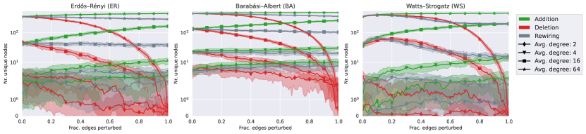
Figure 1: Random edge addition (green), deletion (red), and rewiring (grey) applied to, using the count measure, anonymize ER (top left), BA (top right) and WS (bottom left) graphs with $|V|=500$ and average degree $\in\{2,4,16,64\}$.

The main conclusion from these results is that deletion is more effective than addition or rewiring, confirming what we theorized in Section 5.3. Logically, when all edges are deleted, this results in a graph without edges, making all nodes anonymous. On the contrary, edge addition makes the graph more dense, while for rewiring density remains constant. In many cases addition and rewiring result in a higher uniqueness, which is especially clear for the BA model, and average degree larger than 16 for both the ER and WS models. However, for the WS model, with average degree 16, rewiring performs slightly better than deletion when altering a fraction of 0.2 to 0.5 of the edges. This is likely due to the many nearly identical near-cliques in the generated networks.

While these preliminary results can not rule out that addition and rewiring can be valuable in specific cases, we choose to focus on edge deletion in the remainder of the paper.

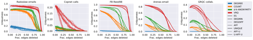
Figure 2: Uniqueness when using different anonymity measures (color) and anonymization algorithms (linestyle) on real-world networks. For each network we show the fraction of deleted edges (horizontal axis) and the attained uniqueness (vertical axis).

6.3 Anonymization and measures

Figure 2 shows how the uniqueness changes when deleting edges using different measures for anonymity, for each of the seven anonymization algorithms. We depict a selection of five networks representative of the overall observed behaviour for the 17 networks listed in Table 2. This is, from left to right in Figure 2, a plateau with a steep decrease, linear decrease, plateau with linear decrease, sigmoid-like decrease and initial increase before decrease. For completeness, the results for the remaining 12 networks are included in Appendix B of the Supplementary materials.

Overall, we see that the measure for anonymity used has a large influence on the results; both on the starting uniqueness with which the process starts and on how quickly the network is anonymized. The simplest measure, degree, has the lowest initial uniqueness and is the easiest to anonymize for. The measure with the furthest reach, vrq, has the highest initial uniqueness, which corresponds to the findings of [25], and is the most difficult to anonymize for.

An example where different measures have the same initial uniqueness but differ in how quickly they are anonymized is the ‘Radoslaw emails’ network. For this network, the uniqueness starts around 0.78 for both count and $d$-$k$-anonymity, but decreases substantially faster for count. Making all nodes anonymous, however, requires a similar amount of edge deletions for both measures.

In the ‘GRQC collab’ network, the results for some anonymization algorithms show an increase before decreasing. This is likely due to the collaboration network’s many cliques. When randomly deleting edges, these cliques are destroyed, which may initially result in higher uniqueness. If edges are targeted more specifically, e.g., using the u-aff-u heuristic, this increase does not occur.

In the remainder of this paper, we focus on the measure count, as this measure is a realistic real-world scenario, has a substantial initial uniqueness compared to the other measures, yet is easier to anonymize for than for example the $d$-$k$-anonymity measure.

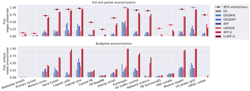
Figure 3: Results for full and partial anonymization (top), where for a network the bar height indicates the fraction of edges that can be preserved when making all nodes anonymous, and the horizontal line indicates the best result obtained for partial anonymization. For Budgeted anonymization (bottom) each bar indicates the fraction of unique nodes anonymized with a budget of 5% of the edges. Color indicates the used anonymization algorithm.

6.4 Full and partial network anonymization

We now turn to the first and second variant of the anonymization problem, aiming to ensure anonymity for 100% and 95% of the nodes in the network. The top of Figure 3 shows which fraction of edges can be preserved when deleting edges until the desired level of anonymity is reached. This fraction equals $\frac{|E^{\prime}|}{|E|}$ where $E$ is the set of edges in the original network, and $E^{\prime}$ in the anonymized network. Here, a higher fraction indicates better results, as preserving more edges overall implies a higher utility of the resulting anonymized network. For the partial variant, both ‘US Power grid’ and ‘Euroroads’ retain 100% of their edges as initially less than 5% of their nodes is unique (so, 95% is already anonymous).

The results show that for some networks, such as ‘Radoslaw emails’ and ‘FB Reed98’ only a small fraction of edges can be preserved, which is also clear from results in Section 6.3. For other networks, larger fractions can be preserved. In these cases, the uniqueness based algorithms, specifically aff-u and u-aff-u, clearly outperform the other algorithms. When dividing the result for the best heuristic by the result of es, we obtain the baseline improvement ratio reported in Table 2. For the full and partial variant, on average 17 and 3.0 times more edges can be preserved.

Moving to the other algorithms, the results show that the structure based algorithms perform similar. For the uniqueness based algorithms, aff-u and u-aff-u perform similar and always achieve better results than the es baseline. However, unique performs worse than the other uniqueness based algorithms.

Turning to the results for anonymizing 95% of the nodes, we see that for some networks a much higher fraction of edges can be preserved. Examples are ‘Moreno health’ and ’Pajek Erdos’. This indicates that these networks contain nodes that are difficult to anonymize and require much attention. When this is the case, one could consider to let more nodes remain unique in order to preserve more edges and therewith achieve an overall higher utility of the resulting anonymized network.

6.5 Budgeted anonymization

We now move to results for the third variant, being budgeted anonymization. As the networks each start at different uniqueness values, as can be seen in Table 2, the values on the vertical axis on the bottom of of Figure 3 show the fraction of unique nodes that is anonymized, i.e., $1-\frac{uniqueness(G^{\prime})}{uniqueness(G)}$, when deleting at most 5% of the edges. A higher value thus indicates that the algorithm is more effective in anonymization within the given budget.

For some of the networks, the anonymization algorithms are quite effective. As can be derived from Table 2, this overall holds for networks with lower initial uniqueness and higher average distance. Experiments to confirm this are included in Appendix C of the Supplementary materials. However, some of the networks, such as ‘Radoslaw emails’ and ‘GRQC collab’, require more than 5% deletion to obtain a substantial decrease in uniqueness. This is also visible in Figure 2 showing a plateau for ‘Radoslaw emails’ and larger initial increase in uniqueness for ‘GRQC collab’.

Overall, we see a big performance difference both between networks and between anonymization algorithms. For some of the networks, such as ‘Moreno health’, ‘Euroroads’, ‘Copnet sms’ or ‘US power grid’, the two best uniqueness based anonymization algorithms, aff-u and u-aff-u, manage to anonymize many more nodes compared to the other algorithms. For all networks, these two uniqueness based algorithms either perform similar or outperform the other algorithms. For the ‘Euroroads’ network, this even results in all nodes being anonymized within the given budget. These algorithms also showed to be most effective for the full and partial variants. On average, 4.4 times more nodes are anonymized compared to the baseline es algorithm. The algorithms especially perform well for networks with a lower initial uniqueness, lower average degree and higher average distance, which is further explained in Appendix C of the Supplementary materials.

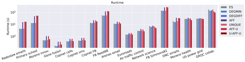
Figure 4: Runtimes for anonymization algorithms (color) with $b=|E|$ and recompute gap $|E|/100$.

6.6 Runtimes

Figure 4 shows the observed runtime of each algorithm on each network by our ANO-NET framework. The runtime consists of both computing probabilities to choose edges and bookkeeping operations, including updating the partition and deleting the chosen edges from the network (line 1 and 1 in Algorithm 1).

The results show that the runtimes vary considerably between networks, which are sorted based on the number of nodes. The first two networks, ‘Radoslaw emails’ and ‘Primary school’, which contain the smallest number of nodes, require more time than the ones following in node size, ‘Moreno innov.’ and ‘Gene fusion’. This is likely due to their high uniqueness throughout the process which makes anonymization more computationally expensive.

Moving to the different algorithms, we first note that the es baseline spends a minimum amount of time on edge selection and hence most time is spent on bookkeeping. Overall, there is no large difference in the runtimes achieved by the algorithms. When comparing the runtimes more closely, uniqueness based algorithms are often slightly more time consuming, as computation of the probability assigned to edges is more expensive. However, for some networks, e.g., ‘Air traffic control’ and ‘Network science’, u-aff-u is slightly faster than the other algorithms, including es. This can likely be explained by the fact that u-aff-u is more effective in anonymization, which results in fewer unique nodes early in the anonymization process. This, in turn, results in lower runtimes for the bookkeeping operations and the edge probability computation.

7 Conclusion

In this paper, we introduced the anonymization problem in networks in the form of three variants being 1) full, 2) partial and 3) budgeted anonymization. We introduced a generic framework coined ANO-NET which allows one to anonymize networks with various settings, including measures for anonymity, different anonymization algorithms and relevant parameters.

Of the anonymization operations that can be applied, results on graph models showed that edge deletion is most effective. We proposed and experimentally evaluated seven measure-agnostic anonymization algorithms, categorized into edge sampling, structure based and uniqueness based approaches. Experiments to assess the effect of different anonymity measures on the anonymization process highlighted how networks are more difficult to anonymize using a more strict measure. The choice in measure affects both the initial uniqueness and how quickly uniqueness decreases.

The effectiveness of the algorithms differed noticeably per network. In particular, networks with lower initial uniqueness and higher average path length, showed to be easier to anonymize. From the anonymization algorithms two of the uniqueness based algorithms which account for the number of unique nodes affected, consistently showed to be most effective for anonymization. Compared to the baseline, the best heuristic algorithm anonymized on average 4.4 times more nodes for the budgeted variant, and preserved 17 and 3.0 times more edges for the full and partial variant. While overall comparable, runtimes for the uniqueness based algorithms appear affected by the initial uniqueness and speed of uniqueness decrease obtained.

The aim of this paper was to present a general version of the anonymization problem and its variants, study various properties of the problem, and evaluate seven relatively simple heuristic algorithms. An obvious next step is to design (metaheuristic) anonymization algorithms, or explore the use of machine learning. Additionally, it would be interesting theoretically to determine the complexity of the problem when using measures such as count or vrq. Lastly, a step forward would be to dynamically account for how data utility decreases during the anonymization process.

Appendix A Recompute gap

This appendix accompanies Section 5.2 of the full paper. Here, we compare the performance and runtimes achieved by the anonymization algorithms when using different recompute gaps. Figure 5 shows the results for different algorithms when using different recompute gaps. The value of 1 implies that values are recomputed after each edge deletion, $|E|/100$ equals the default setting. The figure overall shows that using a smaller recompute gap similar results are obtained. Turning to the runtimes in Figure 6 we see that using a smaller recompute gap does result in larger runtimes.

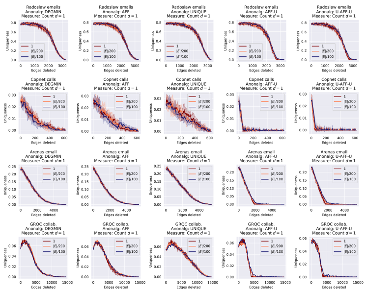
Figure 5: Anonymization process for a selection of networks, anonymization algorithms and different recompute gaps (color).

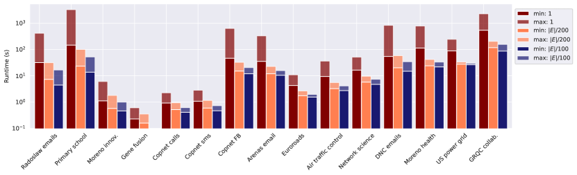
Figure 6: Runtimes for anonymization using different recompute gap values (1, $|E|$/200 and $|E|$/100). Opaque values denote the largest average runtime of the anonymization algorithms, while the solid values denote the lowest value found.

Appendix B Anonymization process

This appendix contains supplementary figures accompanying Section 6.3 up to 6.5 of the full paper. Results shows the full anonymization process, i.e., up to deleting all edges. Figure 7 shows results for all anonymity measures for all networks not shown in Figure 1 of the full paper. Figure 8 shows this process for the count measure.

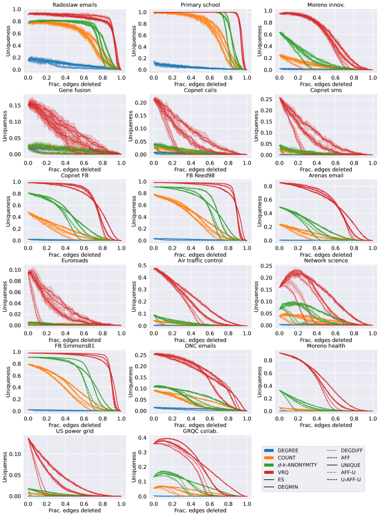
Figure 7: Anonymization process for all networks, anonymization algorithms (line style) and measures (color).

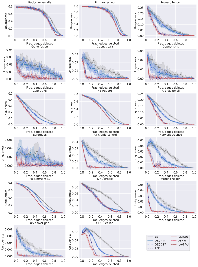
Figure 8: Anonymization process for all networks in Table 2 of the paper and measures (color and linestyle) for count.

Appendix C Properties and anonymization

This appendix accompanies Section 6.3 and 6.4 of the full paper and contains results on correlations between network properties and the effectiveness of the anonymization algorithms on the three variants of the anonymization problem. Table 3 denotes the Pearson correlation and p-value. For combinations deemed significant, Figure 9 shows the values for all networks.

	1. Full		2. Partial		3. Budgeted
Network property	Pearson correlation	p-value	Pearson correlation	p-value	Pearson correlation	p-value
Unique start	-0.86	0.00	-0.92	0.00	-0.76	0.00
$|V|$	0.13	0.62	0.29	0.25	0.06	0.81
Average degree	-0.19	0.45	-0.13	0.61	-0.15	0.56
Median degree	-0.80	0.00	-0.87	0.00	-0.68	0.00
Transitivity	-0.52	0.03	-0.48	0.05	-0.59	0.01
Assortativity	0.15	0.56	0.29	0.25	0.10	0.71
diameter	0.64	0.01	0.60	0.01	0.62	0.01
Average path length	0.65	0.00	0.62	0.01	0.64	0.01

Table 3: Graph properties and correlation with anonymization results. Given various graph measures, denoted in the leftmost column, the Pearson correlation is shown with the best outcomes of the three anonymization variants (second column to last column). For each outcome both the Pearson correlation and $p$-value are given. Values with $p<0.05$ and Pearson correlation larger than 0.4, or smaller than -0.4, are shown in bold.

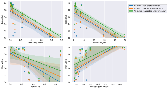
Figure 9: Network properties and anonymization. Each plot shows the the best value obtained (vertical axis) for each anonymization variant (color) on a specific network and the value of a network property (horizontal axis). Combinations plotted are those with a correlation deemed significant as denoted in Table 3.

References

- [1] Asma Azizi, Cesar Montalvo, Baltazar Espinoza, Yun Kang, and Carlos Castillo-Chavez. Epidemics on networks: Reducing disease transmission using health emergency declarations and peer communication. Infectious Disease Modelling, 5:12–22, 2020.
- [2] Wei Chen, Yajun Wang, and Siyu Yang. Efficient influence maximization in social networks. In Proceedings of the 15th ACM SIGKDD international conference on Knowledge discovery and data mining, pages 199–208, 2009.
- [3] Leman Akoglu, Mary McGlohon, and Christos Faloutsos. Oddball: Spotting anomalies in weighted graphs. In Proceedings of the 4th Pacific-Asia Conference on Knowledge Discovery and Data Mining (PAKDD), pages 410–421. Springer, 2010.
- [4] Jure Leskovec, Kevin J. Lang, and Michael Mahoney. Empirical comparison of algorithms for network community detection. In Proceedings of the 19th International Conference on World Wide Web, page 631–640, 2010.
- [5] Lars Backstrom, Cynthia Dwork, and Jon Kleinberg. Wherefore art thou r3579x? anonymized social networks, hidden patterns, and structural steganography. In Proceedings of the 16th International Conference on World Wide Web, page 181–190, 2007.
- [6] Daniele Romanini, Sune Lehmann, and Mikko Kivelä. Privacy and uniqueness of neighborhoods in social networks. Scientific Reports, 11(1):20104, 2021.
- [7] Rachel G. de Jong, Mark P. J. van der Loo, and Frank W. Takes. The effect of distant connections on node anonymity in complex networks. Scientific Reports, 14(1):1156, 2024.
- [8] Xuesong Lu, Yi Song, and Stéphane Bressan. Fast identity anonymization on graphs. In Database and Expert Systems Applications: 23rd International Conference, pages 281–295, 2012.
- [9] Alina Campan and Traian Marius Truta. Data and structural k-anonymity in social networks. In Privacy, Security, and Trust in KDD, pages 33–54, Berlin, Heidelberg, 2009.
- [10] Smriti Bhagat, Graham Cormode, Balachander Krishnamurthy, and Divesh Srivastava. Class-based graph anonymization for social network data. volume 2, page 766–777, aug 2009.
- [11] Changchang Liu and Prateek Mittal. Linkmirage: Enabling privacy-preserving analytics on social relationships. In Proceedings of the 23rd Annual Network and Distributed System Security Symposium, 2016.
- [12] Giorgia Minello, Luca Rossi, and Andrea Torsello. k-anonymity on graphs using the szemerédi regularity lemma. IEEE Transactions on Network Science and Engineering, 8(2):1283–1292, 2020.
- [13] Alessandra Sala, Xiaohan Zhao, Christo Wilson, Haitao Zheng, and Ben Y. Zhao. Sharing graphs using differentially private graph models. In Proceedings of the 2011 ACM SIGCOMM Conference on Internet Measurement Conference, page 81–98, 2011.
- [14] Yue Wang and Xintao Wu. Preserving differential privacy in degree-correlation based graph generation. Transactions on data privacy, 6(2):127, 2013.
- [15] Qian Xiao, Rui Chen, and Kian-Lee Tan. Differentially private network data release via structural inference. In Proceedings of the 20th ACM SIGKDD International Conference on Knowledge Discovery and Data Mining, page 911–920, 2014.
- [16] Davide Proserpio, Sharon Goldberg, and Frank McSherry. Calibrating data to sensitivity in private data analysis: A platform for differentially-private analysis of weighted datasets. Proceedings of the VLDB Endowment, 7(8):637–648, 2014.
- [17] Michael Hay, Vibhor Rastogi, Gerome Miklau, and Dan Suciu. Boosting the accuracy of differentially private histograms through consistency. Proceedings of the VLDB Endowment, 3(1–2):1021–1032, 2010.
- [18] Kamalkumar R Macwan and Sankita J Patel. Node differential privacy in social graph degree publishing. Procedia computer science, 143:786–793, 2018.
- [19] Honglu Jiang, Jian Pei, Dongxiao Yu, Jiguo Yu, Bei Gong, and Xiuzhen Cheng. Applications of differential privacy in social network analysis: A survey. IEEE Transactions on Knowledge and Data Engineering, 35(1):108–127, 2021.
- [20] Kun Liu and Evimaria Terzi. Towards identity anonymization on graphs. In Proceedings of the ACM SIGMOD International Conference on Management of Data, page 93–106, 2008.
- [21] Michael Hay, Gerome Miklau, David Jensen, Don Towsley, and Philipp Weis. Resisting structural re-identification in anonymized social networks. volume 1, page 102–114, aug 2008.
- [22] Lei Zou, Lei Chen, and M. Tamer Özsu. K-automorphism: a general framework for privacy preserving network publication. In Proceedings of the of the 35th VLDB Endowment, volume 2, pages 946–957, 2009.
- [23] Cynthia Dwork, Frank McSherry, Kobbi Nissim, and Adam Smith. Calibrating noise to sensitivity in private data analysis. In Theory of Cryptography, pages 265–284, Berlin, Heidelberg, 2006.
- [24] Randa Aljably, Yuan Tian, Mznah Al-Rodhaan, and Abdullah Al-Dhelaan. Anomaly detection over differential preserved privacy in online social networks. PloS one, 14(4):e0215856, 2019.
- [25] Rachel G. de Jong, Mark P. J. van der Loo, and Frank W. Takes. A systematic comparison of measures for k-anonymity in networks. 2024.
- [26] Sara Rajabzadeh, Pedram Shahsafi, and Mostafa Khoramnejadi. A graph modification approach for k-anonymity in social networks using the genetic algorithm. Social Network Analysis and Mining, 10:1–17, 2020.
- [27] Xiaolin Zhang, Jiao Liu, Jian Li, and Lixin Liu. Large-scale dynamic social network directed graph k-in&out-degree anonymity algorithm for protecting community structure. IEEE Access, 7:108371–108383, 2019.
- [28] Debasis Mohapatra and Manas Ranjan Patra. Graph anonymization using hierarchical clustering. In Computational Intelligence in Data Mining, pages 145–154, 2019.
- [29] Kamalkumar R Macwan and Sankita J Patel. k-degree anonymity model for social network data publishing. Advances in Electrical & Computer Engineering, 17(4):117 – 124, 2017.
- [30] Jordi Casas-Roma, Jordi Herrera-Joancomartí, and Vicenç Torra. An algorithm for k-degree anonymity on large networks. In Proceedings of the 2013 IEEE/ACM international conference on advances in social networks analysis and mining, pages 671–675, 2013.
- [31] Bin Zhou and Jian Pei. Preserving privacy in social networks against neighborhood attacks. In Proceedings of the 24th IEEE International Conference on Data Engineering, pages 506–515, 2008.
- [32] Bin Zhou and Jian Pei. The k-anonymity and l-diversity approaches for privacy preservation in social networks against neighborhood attacks. Knowledge and Information Systems, 28(1):47–77, 2011.
- [33] BK Tripathy and Anirban Mitra. An algorithm to achieve k-anonymity and l-diversity anonymisation in social networks. In 2012 Fourth International Conference on Computational Aspects of Social Networks, pages 126–131, 2012.
- [34] Arash Alavi, Rajiv Gupta, and Zhiyun Qian. When the attacker knows a lot: The gaga graph anonymizer. In Proceedings of the 21st Springer International Conference on Information Security, pages 211–230, 2019.
- [35] Stephen P Borgatti, Kathleen M Carley, and David Krackhardt. On the robustness of centrality measures under conditions of imperfect data. Social networks, 28(2):124–136, 2006.
- [36] Yuchen Li, Ju Fan, Yanhao Wang, and Kian-Lee Tan. Influence maximization on social graphs: A survey. IEEE Transactions on Knowledge and Data Engineering, 30(10):1852–1872, 2018.
- [37] Michael Hay, Gerome Miklau, David Jensen, Philipp Weis, and Siddharth Srivastava. Anonymizing social networks. Computer Science Department Faculty Publication Series, page 180, 2007.
- [38] Akshat Malik, Bram Adams, and Ahmed Hassan. Towards graph-anonymization of software analytics data: empirical study on jit defect prediction. Empirical Software Engineering, 29(4):76, 2024.
- [39] Javier Garcia-Bernardo, Jan Fichtner, Frank W Takes, and Eelke M Heemskerk. Uncovering offshore financial centers: Conduits and sinks in the global corporate ownership network. Scientific Reports, 7(1):1–10, 2017.
- [40] Rachel G. de Jong, Mark P. J. van der Loo, and Frank W. Takes. Algorithms for efficiently computing structural anonymity in complex networks. ACM Journal of Experimental. Algorithmics, 28, 2023.
- [41] Brian Thompson and Danfeng Yao. The union-split algorithm and cluster-based anonymization of social networks. In Proceedings of the 4th International Symposium on Information, Computer, and Communications Security, page 218–227, 2009.
- [42] Sean Chester, Bruce M Kapron, Gautam Srivastava, and Srinivasan Venkatesh. Complexity of social network anonymization. Social Network Analysis and Mining, 3(2):151–166, 2013.
- [43] Albert-Laszlo Barabasi and Zoltan N Oltvai. Network biology: understanding the cell’s functional organization. Nature reviews genetics, 5(2):101–113, 2004.
- [44] Brendan D. McKay and Adolfo Piperno. Practical graph isomorphism, ii. Journal of Symbolic Computation, 60:94–112, 2014.
- [45] Jérôme Kunegis. Konect: the koblenz network collection. In Proceedings of the 22nd International Conference on World Wide Web, page 1343–1350, 2013.
- [46] Sociopatterns. Sociopatterns: Datasets, 2021.
- [47] Piotr Sapiezynski, Arkadiusz Stopczynski, David D. Lassen, and Sune L. Jørgensen. The copenhagen networks study interaction data. figshare. https://doi.org/10.6084/m9.figshare.7267433.v1 (last accessed May 2022), 2019.
- [48] Ryan A. Rossi and Nesreen K. Ahmed. The network data repository with interactive graph analytics and visualization. In Proceedings of the 29th AAAI Conference on Artificial Intelligence, page 4292–4293, 2015.
- [49] Jure Leskovec and Andrej Krevl. Snap datasets: Stanford large network dataset collection. http://snap.stanford.edu/data (last accessed May 2022), 2014.
- [50] Aric Hagberg, Pieter Swart, and Daniel Schult. Exploring network structure, dynamics, and function using networkx. Technical report, Los Alamos National Lab (LANL), 2008.
- [51] Paul Erdős and Alfréd Rényi. On the evolution of random graphs. Publication of the Mathematical Institute of the Hungarian Academy of Sciences, 5(1):17–60, 1960.
- [52] Albert László Barabási and Réka Albert. Emergence of scaling in random networks. Science, 286(5439):509–512, 1999.
- [53] Duncan J. Watts and Steven H. Strogatz. Collective dynamics of ‘small-world’ networks. Nature, 393(6684):440–442, 1998.