Magnetic field effects on electroweak phase transition and baryon asymmetry

Abstract

In the early universe, the first-order phase transition may occur in the background of magnetic fields, leading to baryon number asymmetry through chiral anomaly. We have numerically simulated the first-order electroweak phase transition in the background of a magnetic field in a three-dimensional lattice, discovered the phenomenon of Higgs condensation, and for the first time given the relationship between baryon number asymmetry and magnetic field strength. The magnetic field strength required to achieve the matter-antimatter asymmetry by the evolution of magnetohydrodynamics is about $10^{-17}\sim 10^{-14}$ Gauss at present depending on the correlation length of the helical magnetic field. Our research provides a strong basis for explaining the baryon number asymmetry with cosmic magnetic fields.

I Introduction

Magnetic fields (MFs) are widely present in the solar system, the Milky Way Wielebinski (2005), galaxies and galaxy clusters Clarke et al. (2001); Bonafede et al. (2010); Feretti et al. (2012), and in the voids of large-scale structures Dolag et al. (2010); Tavecchio et al. (2010, 2011); Vovk et al. (2012). MFs are generally believed to result from some primordial MFs generated during the physical processes in the early universe, such as electroweak phase transition (PT) Hogan (1983); Di et al. (2021); Enqvist and Olesen (1993); Yang and Bian (2022); Vachaspati (1991); Baym et al. (1996); Grasso and Riotto (1998), QCD PT Quashnock et al. (1989), and inflation Turner and Widrow (1988); Adshead et al. (2016); Martin and Yokoyama (2008); Kanno et al. (2009); Ratra (1992), and then through an amplification mechanism Grasso and Rubinstein (2001); Widrow (2002); Kulsrud and Zweibel (2008); Kandus et al. (2011); Widrow et al. (2011); Durrer and Neronov (2013). These possible related new physics that seeded the large-scale MF can be probed by gamma-ray observations of blazars Dermer et al. (2011); Taylor et al. (2011); Neronov and Vovk (2010).

Previous studies show that the appearance of the MF will affect the Higgs vacuum, making it present a vortex structure, the Ambjørn-Olesen condense Nielsen and Olesen (1978); MacDowell and Törnkvist (1992); Salam and Strathdee (1975); Linde (1976); Ambjørn (1989); Chernodub et al. (2023). More importantly, the Chern-Simons Number stored in the MF will be converted into baryon number through chiral anomaly, thereby realizing baryon number asymmetry of the Universe (BAU) Giovannini and Shaposhnikov (1998a, b); Joyce and Shaposhnikov (1997). It is worth studying whether this phenomenon still exists under the first-order electroweak PT occurring in the early Universe predicted by beyond the standard model new physics Hindmarsh et al. (2021); Caldwell et al. (2022); Athron et al. (2024). Such a PT can provide an equilibrium departure environment to explain the problem of BAU through the electroweak baryogenesis Morrissey and Ramsey-Musolf (2012); Cohen et al. (2012) and source an important stochastic gravitational wave backgrounds Mazumdar and White (2019); Caprini et al. (2016, 2020) to be probed by future space-based gravitational wave detectors such as Laser Interferometer Space Antenna (LISA) Amaro-Seoane et al. (2017), TianQin Luo et al. (2016), Taiji Ruan et al. (2020).

Therefore, in this Letter, we intend to use numerical methods to simulate the first-order electroweak PT under MF backgrounds, analyze the influence of MF on the PT, give the quantitative relationship between baryon number asymmetry and MF for the first time, and analyze the MF strength of present which can achieve the correct matter-antimatter asymmetry. For generic, we here consider both the helical MF of infinite correlation length and the helical MF with electroweak PT characteristic correlation length.

This letter uses the natural unit $\hbar=c=k_{\mathrm{B}}=1$. Since the PT completed very fast, we ignore the expansion of the universe, the evolution of the external MF, and the change in temperature.

II The Setup

We adopt the Lagrangian of the electroweak theory with an extra U(1) field $Y_{\mathrm{ex}}^{\mu}$ whose strength $Y_{\mathrm{ex}}^{\mu\nu}$ does not change over time,

$$\mathcal{L}=\ (D_{\mu}\Phi)^{\dagger}(D^{\mu}\Phi)-\frac{1}{4}W^{a}_{\mu\nu}W^{a\mu\nu}-\frac{1}{4}Y_{\mu\nu}Y^{\mu\nu}$$

$$\ -\frac{1}{2}Y^{\mathrm{ex}}_{\mu\nu}Y^{\mu\nu}+\mathcal{V}(\Phi)\;.$$ (1)

Here $\Phi$ represents the Higgs doublet, $W^{a}_{\mu\nu}$ and $Y_{\mu\nu}$ represents the $\mathrm{SU(2)_{L}}$ and $\mathrm{U(1)_{Y}}$ gauge field strength, respectively. The covariant derivative is

$$D_{\mu}=\partial_{\mu}-\mathrm{i}g\frac{\sigma^{a}}{2}W_{\mu}^{a}-\mathrm{i}g^{\prime}\,\frac{1}{2}(Y_{\mu}+Y^{\mathrm{ex}}_{\mu}),$$ (2)

where $\sigma^{a},\ a=1,\ 2,\ 3$ is Pauli matrix, $g=0.65$ and $g^{\prime}=0.53g$. $W^{\mu}$ and $Y^{\mu}=(Y^{0},\ \boldsymbol{Y})$ is the $\mathrm{SU(2)_{L}}$ and $\mathrm{U(1)_{Y}}$ gauge field, respectively. We omit $Y^{\mathrm{ex}}_{\mu\nu}Y^{\mu\nu}_{\mathrm{ex}}$ since it is a constant. The potential $\mathcal{V}(\Phi)$ contains a potential barrier and admits a first-order electroweak PT, given by

$$\mathcal{V}(\Phi) =-\mu^{2}\Phi^{\dagger}\Phi+A(\Phi^{\dagger}\Phi)^{3/2}+\lambda(\Phi^{\dagger}\Phi)^{2}\;.$$ (3)

The nucleated bubble will expand and collide with one another to propel the PT process with the initial bubble profile being obtained using the FindBounce Guada et al. (2020). See the Equations of Motion on Lattice and Initialization section in the supplemental material for the specific form of discrete models.

The MF is not well defined before the electroweak PT occurs we therefore use an extra external hyperMF $\boldsymbol{B}^{\mathrm{ex}}_{Y}=\nabla\times\boldsymbol{Y}^{\mathrm{ex}}$ instead of MF $\boldsymbol{B}^{\mathrm{ex}}=\nabla\times\boldsymbol{A}^{\mathrm{ex}}$ Chernodub et al. (2023), where $\boldsymbol{Y}^{\mathrm{ex}}$ is the space part of U(1) gauge field $Y^{\mu}_{\mathrm{ex}}=(Y^{0}_{\mathrm{ex}},\ \boldsymbol{Y}_{\mathrm{ex}})$ and $\boldsymbol{A}_{\mathrm{ex}}$ is the space part of electroMF $A^{\mu}_{\mathrm{ex}}=(A^{0}_{\mathrm{ex}},\ \boldsymbol{A_{\mathrm{ex}}})$. In the broken phase, the relation between the two fields is $g^{\prime}\boldsymbol{B}_{Y}^{\mathrm{ex}}=e\boldsymbol{B}^{\mathrm{ex}}$, here $e=g\sin\theta_{w}$ is the electric charge.

In this Letter, we consider two types of hyperMFs with different correlation lengths, which are defined as $\lambda_{BY}=\int\mathrm{d}k\,k^{-1}E_{BY}(k)\ \Big{/}\int\mathrm{d}k\,E_{BY}(k)$, where $\int\mathrm{d}k\,E_{BY}(k)=\int\mathrm{d}^{3}\boldsymbol{x}\,\frac{1}{2}[\boldsymbol{B}^{\mathrm{ex}}_{Y}(\boldsymbol{x})]^{2}/V$. To consider an infinite correlation length hyperMF with helicity, for simplicity we let $Y^{\mathrm{ex}\mu}=(0,\ 0,\ xB_{Y}^{\mathrm{ex}},\ h_{\mathrm{factor}}LB_{Y}^{\mathrm{ex}})$, where $h_{\mathrm{factor}}$ is an adjustable parameter in $[-1,\ 1]$, $L=N\Delta x$ is the edge length of the lattice box. For the finite correlation length hyperMF, we consider Brandenburg et al. (2020a) $\tilde{B}_{Yi}^{\mathrm{ex}}(\boldsymbol{k})=B_{\mathrm{ini}}\Theta(k-k_{\mathrm{UV}})\left(\delta_{ij}-\hat{k}_{i}\hat{k}_{j}-\mathrm{i}\sigma_{\mathrm{M}}\varepsilon_{ijl}\hat{k}_{l}\right)g_{j}(\boldsymbol{k})k^{n}$, where $\Theta(k-k_{\mathrm{UV}})$ is the Heaviside function to make the hyperMF have a finite correlation length comparable with the mean bubble separation $R^{*}=(V/N_{\mathrm{bubble}})^{1/3}$ when the vacuum bubbles percolation process proceeds during the PT, $k_{\mathrm{UV}}$ is the ultraviolet cutoff wave number $k_{\mathrm{UV}}$, and $\boldsymbol{g}(\boldsymbol{k})$ is the Fourier transform of a Gaussian distributed random vector field that is $\delta$-correlated in all three dimensions, i.e., $g_{i}(\boldsymbol{x})g_{j}(\boldsymbol{x}^{\prime})=\delta_{ij}\delta^{3}(\boldsymbol{x-x^{\prime}})$. $n$ is the index of the spectrum. The degree of helicity is controlled by the parameter $\sigma_{\mathrm{M}}=0,1,-1$ for non-helical, maximally positive and negative helicity, respectively. The specific implementation method of hyperMF on lattice is shown in the Hypermagenetic Field on Lattice section in the supplemental material.

According to the chiral anomaly in the electroweak theory, the relationship between fermions and gauge fields is as follows Adler (1969); Bell and Jackiw (1969); ’t Hooft (1976a, b):

$$\partial_{\mu}j_{\mathrm{B}}^{\mu}=N_{\mathrm{g}}\left[\frac{g^{2}}{16\pi^{2}}\mathrm{Tr}\,(W_{\mu\nu}\tilde{W}^{\mu\nu})-\frac{g^{\prime 2}}{32\pi^{2}}Y_{\mu\nu}\tilde{Y}^{\mu\nu}\right],$$ (4)

where $N_{\mathrm{g}}=3$ is the number of families of fermions. Integrating it in finite time and infinite volume, we get

$$\Delta n_{\mathrm{B}}=N_{\mathrm{g}}\frac{\Delta N_{\mathrm{CS}}(t)}{V}=N_{\mathrm{g}}\frac{N_{\mathrm{CS}}(t)-N_{\mathrm{CS}}(0)}{V},$$ (5)

where

$$\frac{N_{\mathrm{CS}}(t)}{V}=\frac{1}{V}\frac{1}{32\pi^{2}}\varepsilon^{ijk}\int\mathrm{d}^{3}x\biggl{[}-g^{\prime 2}(Y_{i}+Y^{\mathrm{ex}}_{i})(Y_{jk}+Y^{\mathrm{ex}}_{jk})+g^{2}\left(W^{a}_{i}W^{a}_{jk}-\frac{g}{3}\varepsilon^{abc}W^{a}_{i}W^{b}_{j}W^{c}_{k}\right)\biggr{]}$$ (6)

is Chern-Simons number Moore (2002) which is closely related to the baryon number density $n_{\mathrm{B}}$, and $V=L^{3}$ is the lattice volume. The U(1) part of $N_{\mathrm{CS}}$ is hypermagnetic helicity

$$h_{Y}=\frac{H_{Y}}{V} =\frac{1}{V}\varepsilon^{ijk}\int\mathrm{d}x^{3}\ (Y_{i}+Y_{i}^{\mathrm{ex}})(Y_{jk}+Y_{jk}^{\mathrm{ex}})$$

$$=\frac{1}{V}\int\ \mathrm{d}x^{3}(\boldsymbol{Y}+\boldsymbol{Y}^{\mathrm{ex}})\cdot(\boldsymbol{B}_{Y}+\boldsymbol{B}^{\mathrm{ex}}_{Y}),$$ (7)

up to a negative factor.

When the helicity of the external hyperMF is not $0$, that is, $\boldsymbol{Y}^{\mathrm{ex}}\cdot\boldsymbol{B}^{\mathrm{ex}}_{Y}\neq 0$, during the PT, the bubble collision will generate a MF Di et al. (2021), which causes $\boldsymbol{Y}\cdot\boldsymbol{B}_{Y}$, $\boldsymbol{Y}\cdot\boldsymbol{B}^{\mathrm{ex}}_{Y}$ and $\boldsymbol{Y}^{\mathrm{ex}}\cdot\boldsymbol{B}_{Y}$ to be non-zero during the PT, which is reflected in the changes of $h_{Y}$ and $N_{\mathrm{CS}}$. Moreover, the greater the strength and helicity of the external hyperMF, the greater the increase in the latter two terms, and the more drastic and large the change will be.

We use diffusion rate Tranberg and Smit (2003) which is also known as the sphaleron rate

$$\Gamma(t)=\frac{1}{V}\frac{\mathrm{d}}{\mathrm{d}t}[\langle(\Delta N_{\mathrm{CS}}(t))^{2}\rangle-\langle\Delta N_{\mathrm{CS}}(t)\rangle^{2}]$$ (8)

to measure the intensity of the change of $N_{\mathrm{CS}}$. It is a time-varying quantity in non-equilibrium, and it is the slope of a straight line $\langle(\Delta N_{\mathrm{CS}})^{2}\rangle-\langle\Delta N_{\mathrm{CS}}\rangle^{2}$ in equilibrium. The angle brackets indicate averaging over multiple runs. Based on $\Gamma(t)$, we define the time-averaged sphaleron rate:

$$\bar{\Gamma}(t)=\frac{1}{t-t_{0}}\int_{t_{0}}^{t}\mathrm{d}t^{\prime}\,\Gamma(t^{\prime}).$$ (9)

Last but not least, the physical quantity that measures the baryon number density in the universe is $\eta_{\mathrm{B}}=n_{\mathrm{B}}/s\sim 10^{-10}$, which is a constant if particles are neither produced nor destroyed. $s=2\pi^{2}g_{*S}T^{3}/45$ is the entropy density. $g_{*S}$ is the effective number of degrees of freedom in entropy, which is equal to $106.75$ before the electroweak PT. Combining the above equations, we get the relationship between $\eta_{\mathrm{B}}$ and $N_{\mathrm{CS}}$:

$$\Delta\eta_{\mathrm{B}}=\frac{45N_{\mathrm{g}}}{2\pi^{2}g_{*S}T^{3}}\frac{\Delta N_{\mathrm{CS}}(t)}{V}=0.064\frac{1}{T^{3}}\frac{\Delta N_{\mathrm{CS}}(t)}{V}.$$ (10)

III Numerical Results

We perform numerical simulations on a discrete three-dimensional lattice of size $N^{3}=128^{3}$ with lattice spacing $\Delta x$ and periodic boundary conditions using real-time evolution. The time interval $\Delta t=\Delta x/5$. We perform 20 runs for each set of MFs or helicity with other parameters being fixed and average the data.

III.1 Helical hypermagnetic fields of infinite correlation length

It is proposed that when the MF increases beyond the first critical value $g^{\prime}B_{Y\mathrm{c1}}=eB_{\mathrm{c1}}=m_{W}^{2}$ where $m_{W}$ is the mass of the W boson, in order to stabilize the vacuum, the Higgs field will form a hexagonally arranged vortex, which is called Ambjørn-Olesen condense Nielsen and Olesen (1978); MacDowell and Törnkvist (1992); Salam and Strathdee (1975); Linde (1976). Recently, the theoretical proposal has been numerically confirmed by Ref. Chernodub et al. (2023) for the SM cross-over case.

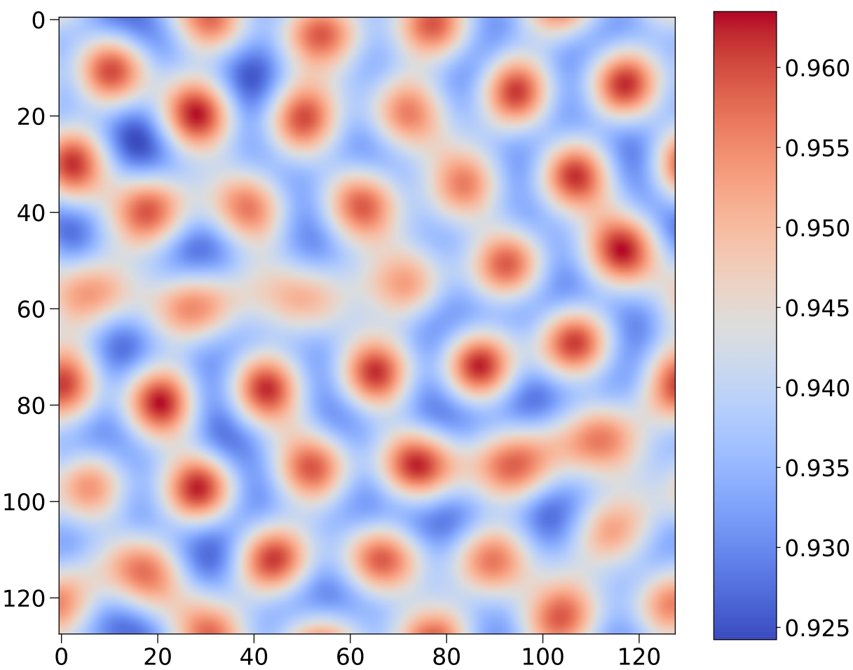
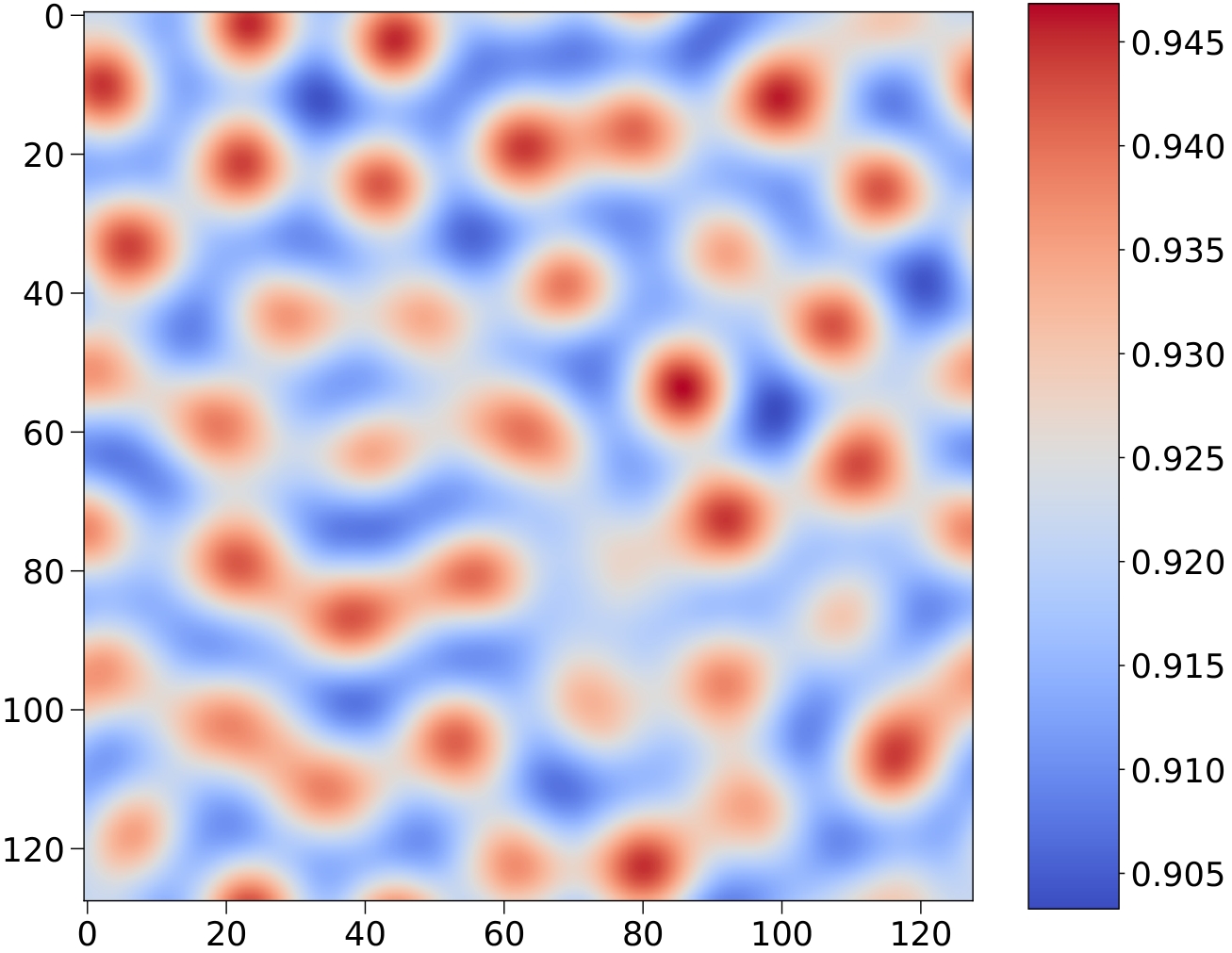
Figure 1: $\bar{\Phi}^{2}$ under non-helical(Left) and helical(Right) homogeneous hyperMF $g^{\prime}B_{Y}/m_{W}^{2}=3.63$. When $g^{\prime}B_{Y}/m_{W}^{2}$ exceeds the critical value which is approximately $3$, Higgs condensation begins to appear whether the hyperMF is helical or not.

We first examine the effect of helical MF on the first-order electroweak PT process. To eliminate fluctuations in space and time and make the image clearer, what we show in Fig. 1 is $\bar{\Phi}^{2}(x,y)=\frac{1}{NN_{t}}\sum_{t,z}\Phi^{2}(t,x,y,z)$, where the time average is from the completion of the PT to the end of the simulation. We show that the Higgs condensation occurs when $g^{\prime}B_{Y}/m_{W}^{2}\gtrsim 3$ no matter whether the MF is helical or non-helical. We also found that as the hyperMF increases, the vortices become more and more dense, and the hyperMF always slows down the expansion of the vacuum bubble, which leads to the nucleation of more bubbles and a slower PT, see the Phase Transition and Ambjørn-Oleson Cendense section in the supplemental material.

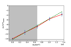
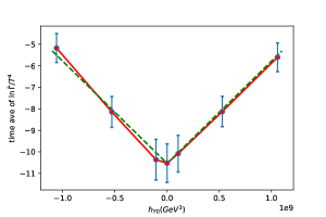
Figure 2: Top: Changes of $(\ln\,\bar{\Gamma}(t)/T^{4})_{\mathrm{stable}}$ over different homogeneous, helical MFs. The gray line represents the value of the sphaleron rate in the symmetric phase $\Gamma_{\mathrm{sym}}/T^{4}=6.23\times 10^{-7}$ Annala and Rummukainen (2023). The gray area indicates the magnetic field strength where Higgs condensation has not yet occurred. Bottom: Changes of $(\ln\,\bar{\Gamma}(t)/T^{4})_{\mathrm{stable}}$ over different initial helicity with homogeneous hyperMF fixed at $g^{\prime}B_{Y}/m_{W}^{2}=5.45$. The fitting result of Eq. (11) is represented by the green dashed line.

We now study the EW sphaleron rate behavior under the impact of the homogeneous helical MF. We find that a stronger helical hyperMF background will bring about a more drastic change in $N_{\mathrm{CS}}$, which is reflected by the behavior of $\ln\bar{\Gamma}(t)/T^{4}$, see Fig. 13 in the Electroweak Sphaleron During the Phase Transition under Hypermagnetic Field section of the supplemental material. We here calculate its time average for different hyperMF when it is stable after $t/R*>2.67$, denoted as $(\ln\bar{\Gamma}(t)/T^{4})_{\mathrm{stable}}$, as shown in Fig. 2. As the MF and helicity increase, $(\ln\bar{\Gamma}(t)/T^{4})_{\mathrm{stable}}$ also increases. Note that our initial $Y_{\mathrm{ex}}$ and hyperMF settings for the helical situation are as shown in The Setup section, so the initial helicity is $h_{Y0}=h_{\mathrm{factor}}L(B^{\mathrm{ex}}_{Y})^{2}$. When the hyperMF strength is changed, the helicity $h_{Y0}$ will change simultaneously. Therefore, We can fit the dependence of $(\ln\bar{\Gamma}(t)/T^{4})_{\mathrm{stable}}$ on MF and helicity:

$$\left(\ln\frac{\bar{\Gamma}(t)}{T^{4}}\right)_{\mathrm{stable}}=48*\left(\frac{h_{Y0}}{10^{9}\,\mathrm{GeV}^{3}}\right)\left(\frac{10^{4}\,\mathrm{GeV}^{2}}{B_{Y}}\right)+\ln\frac{\Gamma_{\mathrm{sym}}}{T^{4}}\left[1-0.026\left(\frac{B_{Y}}{10^{4}\,\mathrm{GeV}^{2}}\right)\right]\;,$$ (11)

which is shown in Fig. 2 by the green dashed line.

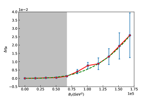
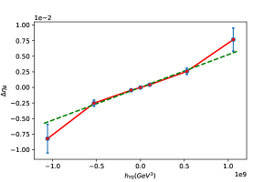
Figure 3: $\Delta\eta_{\mathrm{B}}$ changes with helical external homogeneous hyperMF strength whose $h_{\mathrm{factor}}=1$ (top) and different initial $h_{Y}$ with $g^{\prime}B_{Y}/m_{W}^{2}=5.45$ (bottom). The green dashed line is the fitting result of (12). The gray area indicates the magnetic field strength where Higgs condensation has not yet occurred.

Now we turn our attention to baryon asymmetry. Fig. 3 shows how $\Delta\eta_{\mathrm{B}}$ changes versus hyperMF strength. The top panel reflects that when the hyperMF strength increases, $\Delta\eta_{\mathrm{B}}$ also increases, indicating that more baryons are produced. And, in the bottom panel, we study the change of hyperMF helicity when its strength is fixed. We set $g^{\prime}B_{Y}/m_{W}^{2}=5.45$, and change the $h_{\mathrm{factor}}$ (equal to $0$, $\pm 0.1$, $\pm 0.5$, $\pm 1.0$ respectively) to obtain different initial helicity $h_{Y0}$. When the initial helicity is greater than $0$, it means that the initial $N_{\mathrm{CS}}$ is less than $0$. Then as the PT occurs, $N_{\mathrm{CS}}$ begins to change in the direction towards 0. And the larger the absolute value of the initial helicity $h_{Y0}$, the larger the $\Delta\eta_{\mathrm{B}}\propto\Delta N_{\mathrm{CS}}$. When the PT is completed, the $\Delta N_{\mathrm{CS}}$ is also stable, which means $\eta_{\mathrm{B}}$ is stable as well. We fit the data points in the two plots in Fig. 3 with the green dashed line

$$\eta_{B}=5.2\times 10^{-4}\left(\frac{B_{Y}}{10^{4}\,\mathrm{GeV}^{2}}\right)\left(\frac{h_{Y0}}{10^{9}\,\mathrm{GeV}^{3}}\right),$$ (12)

and find that $\eta_{\mathrm{B}}$ is proportional to $B_{Y}\times h_{Y0}$. Meanwhile, it indicates that the trend of $\Delta\eta_{\mathrm{B}}$ has the same sign of the initial helicity or $h_{\mathrm{factor}}$.

III.2 Hypermagnetic fields with finite correlation length

In the last section, we study the scenario of homogeneous hyperMF, that is, the correlation length of the MF $\lambda_{B}\rightarrow\infty$. The fitting results are also only applicable to this case. Now, we discuss the scenario of finite correlation length close to the mean bubble separation during the electroweak PT.

To study the finite correlation length hyperMF effects on first-order electroweak PT, we simulate four different hyperMF strengths and correlation length by adjusting the spectral index $n$, and each strength included three cases of $\sigma_{\mathrm{M}}=0,\pm 1$. When $k_{\mathrm{UV}}=2\Delta k$, the MF (comoving) correlation lengths obtained for different $n$ are close.

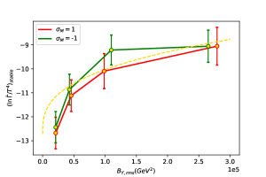
Figure 4: Changes of $(\ln\,\bar{\Gamma}(t)/T^{4})_{\mathrm{stable}}$ over different hypermagnetic energy with $\sigma_{\mathrm{M}}=\pm 1$. The yellow dashed line represents the fitting result of Eq. (13).

Similarly, we extract $(\ln\,\bar{\Gamma}/T^{4})_{\mathrm{stable}}$ as a representative value and plot the variation of electroweak Sphaleron rate versus hyperMF strength in Fig. 4, and use the yellow dashed line to show the following fitting results:

$$\left(\ln\frac{\bar{\Gamma}(t)}{T^{4}}\right)_{\mathrm{stable}}=2.1\left(\frac{B_{Y\mathrm{,rms}}}{10^{4}\ \mathrm{GeV}}\right)^{0.28}+\ln\frac{\Gamma_{\mathrm{sym}}}{T^{4}}\;.$$ (13)

This shows that the electroweak sphaleron rate increases as the strength of the helical MF increases.

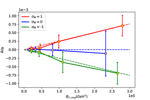
Figure 5: The variation of $\Delta\eta_{\mathrm{B}}$ with different spactral index $n$ or different hypermagnetic energy. The dashed line is the fitting result of (14).

Finally, We check that When the MF energy increases, the $\Delta\eta_{\mathrm{B}}$ of $\sigma_{\mathrm{M}}=\pm 1$ deviates significantly from $0$ again through PT, while the $\Delta\eta_{\mathrm{B}}$ of $\sigma_{\mathrm{M}}=0$ remains near $0$ since there is no helical MF effects here. The dashed line is the result of the following fit

$$\eta_{\mathrm{B}}=2.54\times 10^{-5}\sigma_{\mathrm{M}}\left(\frac{B_{Y\mathrm{,rms}}}{10^{4}\,\mathrm{GeV}^{2}}\right)\;.$$ (14)

With the help of two fitting formulas Eq. (12) and Eq. (14), we can calculate today’s MF strength and MF correlation length required to achieve $\eta_{\mathrm{B}}\sim 10^{-10}$. The specific calculations are provided in the Hypermagnetic Fields and Matter-Antimatter Asymmetry section of supplemental material.

The helicity $h_{Y}$ is closely related to the lepton asymmetry due to the chiral anomaly Boyarsky et al. (2012):

$$\frac{\partial(n_{R}-n_{L})/s}{\partial t}=\frac{T^{2}}{6s}\frac{d\Delta\mu}{dt}=-\frac{\alpha}{\pi s}\frac{\mathrm{d}h_{Y}}{\mathrm{d}t}\;,$$ (15)

where $\alpha$ is the fine-structure constant, and $\Delta\mu=\mu_{R}-\mu_{L}$ is the difference of left and right chemical potentials. We numerically checked that the $B-L$ conservation, in the Chiral Potential and Lepton Asymmetry section of supplemental material.

IV Conclusions

In this Letter, we numerically study the first-order electroweak PT under the background of hyperMF. We find that the hyperMF always slows down the speed of the first-order electroweak PT and the hyperMF with infinite correlation length induces the Ambjørn-Olesen condensation when $g^{\prime}B_{Y}/m_{W}^{2}\gtrsim 3$. However, Due to the randomness of the hyperMF with finite correlation length, the Ambjørn-Olesen condensation phenomenon cannot be observed. Our results reveal that the electroweak Sphaleron rate increased significantly under the strong hyperMF background and show that the PT occurring under the hyperMF background produces a more intense MF generation process, thus affecting the U(1) part of $N_{\mathrm{CS}}$(6). We further observe that the larger the helicity of the background hyperMF, the more net baryons are generated. Based on this, we give the relation between baryon asymmetry and hyperMF. For the infinite correlation length scenario (homogeneous hyperMF), $\eta_{\mathrm{B}}$ is proportional to $B_{Y}$ and $h_{Y}$ ($h_{Y}$ is proportional to $B_{Y}^{2}$ in the simulation), and for the finite correlation length case, $\eta_{\mathrm{B}}$ is solely proportional to $B_{Y}$.

Based on these results, we find that, to achieve the correct matter-antimatter asymmetry, the background homogeneous MF should be $3.5\times 10^{-17}$ Gauss at present, and the spectrum distributed MF should be $4.8\times 10^{-15}$ Gauss with a correlation length of $2.4\times 10^{-4}$ Mpc, that can be probed by Fermi-LAT gamma-ray observations.

We hope that our numerical results can help future observations of the cosmic MF and reveal new physics behind that. It should be emphasized that our simulation considers the first-order PT does not take into account the expansion of the universe and relativistic fluid, and the impact of these two factors on the first-order electroweak PT, these contents deserve future research of the community. In addition, the gravitational waves generated by PTs in the background MFs might be different from those in non-magnetic backgrounds, which is also a direction worth exploring.

Supplemental Material

V Equations of Motion on Lattice

Under the temporal gauge $W_{0}=Y_{0}=Y^{\mathrm{ex}}_{0}=0$, the equations of motion derived from (1) are:

$$\partial_{0}^{2}\Phi\hphantom{{}_{i}}= D_{i}D_{i}\Phi-\frac{\partial\mathcal{V}}{\partial\Phi^{\dagger}}$$

$$\partial_{0}^{2}W^{a}_{i}= -\partial_{k}W^{a}_{ik}-g\epsilon^{abc}W^{b}_{k}W^{c}_{ik}+g\text{Im}[\Phi^{\dagger}\sigma^{a}(D_{i}\Phi)]$$

$$\partial_{0}^{2}Y_{i}= -\partial_{k}Y_{ik}+g^{\prime}\text{Im}[\Phi^{\dagger}(D_{i}\Phi)],$$ (16)

along with two Gauss constraints,

$$\partial_{0}\partial_{j}Y_{j}-g^{\prime}\text{Im}\big{[}\Phi^{\dagger}\partial_{0}\Phi\big{]}=0$$

$$\partial_{0}\partial_{j}W^{a}_{j}+g\epsilon^{abc}W^{b}_{j}\partial_{0}W^{c}_{j}-g\text{Im}\big{[}\Phi^{\dagger}\sigma^{a}\partial_{0}\Phi\big{]}=0.$$ (17)

The Higgs field $\Phi$ is defined on the lattice sites while the gauge fields are defined on the links between two adjacent sites by link fields:

$$U_{i}(t,x) =\exp\left[-\mathrm{i}g\Delta x\frac{\sigma^{a}}{2}W_{i}^{a}(t,x)\right]$$ (18)

$$V_{i}(t,x) =\exp\left[-\mathrm{i}g^{\prime}\Delta x\,\frac{1}{2}Y_{i}(t,x)\right]$$ (19)

$$V^{\mathrm{ex}}_{i}(t,x) =\exp\left[-\mathrm{i}g^{\prime}\Delta x\,\frac{1}{2}Y^{\mathrm{ex}}_{i}(t,x)\right],$$ (20)

Higgs field and gauge fields are defined on the exact time step, and their canonical momenta $\Pi,\ E,\ F$ are defined on the halfway between the time steps.

The action on the lattice is

$$S = \sum_{x,t}\Delta t\Delta x^{3}\Bigg{\{}\big{(}D_{0}\Phi\big{)}^{\dagger}\big{(}D_{0}\Phi\big{)}-\sum_{i}\big{(}D_{i}\Phi\big{)}^{\dagger}\big{(}D_{i}\Phi\big{)}-\mathcal{V}(\Phi)+\Big{(}\frac{2}{g\Delta t\Delta x}\Big{)}^{2}\sum_{i}\Big{(}1-\frac{1}{2}\text{Tr}\leavevmode\nobreak\ U_{0i}\Big{)}$$ (21)

$$+\Big{(}\frac{2}{g^{\prime}\Delta t\Delta x}\Big{)}^{2}\sum_{i}\Big{(}1-\text{Re}\leavevmode\nobreak\ V_{0i}\Big{)}-\frac{2}{g^{2}\Delta x^{4}}\sum_{i,j}\Big{(}1-\frac{1}{2}\text{Tr}\leavevmode\nobreak\ U_{ij}\Big{)}-\frac{2}{g^{\prime 2}\Delta x^{4}}\sum_{i,j}\Big{(}1-\text{Re}\leavevmode\nobreak\ V_{ij}\Big{)}\Bigg{\}}$$

$$+\Big{(}\frac{2}{g^{\prime}\Delta t\Delta x}\Big{)}^{2}\sum_{i}\Big{(}\mathrm{Im}\leavevmode\nobreak\ V_{0i}\Big{)}\Big{(}\mathrm{Im}\leavevmode\nobreak\ V_{\mathrm{ex}0i}\Big{)}-\frac{2}{g^{\prime 2}\Delta x^{4}}\sum_{i,j}\Big{(}\mathrm{Im}\leavevmode\nobreak\ V_{ij}\Big{)}\Big{(}\mathrm{Im}\leavevmode\nobreak\ V_{\mathrm{ex}ij}\Big{)}.$$

We use $x+i$ to denote a space step forward towards the $i$ direction and $x-i$ to denote a space step backward. The link fields, $U_{i}(t,x),\ V_{i}(t,x),\ V^{\text{ex}}_{i}(t,x)$, parallel transport the Higgs field $\Phi$ that located at site $x+i$ back to site $x$; and their hermitian conjugate parallel transport the Higgs field $\Phi$ that located at site $x$ to site $x+i$. Therefore, Using the leapfrog algorithm, the covariant derivative of $\Phi(t,x)$ is

$$D_{i}\Phi =\frac{1}{\Delta x}\big{[}U_{i}(t,x)V_{i}(t,x)V_{\mathrm{ex}i}(t,x)\Phi(t,x+i)-\Phi(t,x)\big{]}$$

$$D_{0}\Phi =\frac{1}{\Delta t}\big{[}U_{0}(t,x)V_{0}(t,x)V_{\mathrm{ex}0}(t,x)\Phi(t+\Delta t,x)-\Phi(t,x)\big{]}$$

$$=\frac{1}{\Delta t}\big{[}\Phi(t+\Delta t,x)-\Phi(t,x)\big{]}.$$

The plaquette fields with all space indices are

$$U_{ij}(t,x) =U_{j}(t,x)U_{i}(t,x+j)U_{j}^{\dagger}(t,x+i)U_{i}^{\dagger}(t,x)$$

$$V_{ij}(t,x) =V_{j}(t,x)V_{i}(t,x+j)V_{j}^{\dagger}(t,x+i)V_{i}^{\dagger}(t,x)$$

$$V_{\mathrm{ex}ij}(t,x) =V_{\mathrm{ex}j}(t,x)V_{\mathrm{ex}i}(t,x+j)V_{\mathrm{ex}j}^{\dagger}(t,x+i)V_{\mathrm{ex}i}^{\dagger}(t,x)$$

The plaquette fields with one time indices are

$$U_{0i}(t,x) =U_{i}(t,x)U_{0}(t+\Delta t,x)U_{i}^{\dagger}(t+\Delta t,x)U_{0}^{\dagger}(t,x)=U_{i}(t,x)U_{i}^{\dagger}(t+\Delta t,x)$$

$$V_{0i}(t,x) =V_{i}(t,x)V_{0}(t+\Delta t,x)V_{i}^{\dagger}(t+\Delta t,x)V_{0}^{\dagger}(t,x)=V_{i}(t,x)V_{i}^{\dagger}(t+\Delta t,x)$$

$$V_{\mathrm{ex}0i}(t,x) =V_{\mathrm{ex}i}(t,x)V_{\mathrm{ex}0}(t+\Delta t,x)V_{\mathrm{ex}i}^{\dagger}(t+\Delta t,x)V_{\mathrm{ex}0}^{\dagger}(t,x)=V_{\mathrm{ex}i}(t,x)V_{\mathrm{ex}i}^{\dagger}(t+\Delta t,x)$$

As we said above, the fields $\Phi(t,x)$, $U_{i}(t,x)$ and $V_{i}(t,x)$ are defined at the exact time steps $t+\Delta t$, $t+2\Delta t$, $\ldots$; while their canonical momenta, $\Pi(t+\Delta t/2,x)$, $F(t+\Delta t/2,x)$ and $E(t+\Delta t/2,x)$, are defined at half-way time steps $t+\Delta t/2$, $t+3\Delta t/2$, $\ldots$. They are related by

$$\Phi(t+\Delta t,x) =\Phi(t,x)+\Delta t\Pi(t+\Delta t/2,x)$$ (22)

$$V_{i}(t+\Delta t,x) =\frac{1}{2}g^{\prime}\Delta x\Delta tE_{i}(t+\Delta t/2,x)V_{i}(t,x)$$ (23)

$$U_{i}(t+\Delta t,x) =g\Delta x\Delta tF_{i}(t+\Delta t/2,x)U_{i}(t,x),$$ (24)

$V_{\mathrm{ex}i}(t,x)$ does not change over time, so we don’t need its canonical momentum $E_{\mathrm{ex}i}(t,x)$.

The equations of motion that result from setting the functional derivative of the action to zero are:

$$\Pi(t+\Delta t/2,x)= \ \Pi(t-\Delta t/2,x)+\Delta t\Big{\{}\frac{1}{\Delta x^{2}}\sum_{i}\big{[}U_{i}(t,x)V_{i}(t,x)V_{\mathrm{ex}i}(t,x)\Phi(t,x+i)$$

$$-2\Phi(t,x)+U_{i}^{\dagger}(t,x-i)V_{i}^{\dagger}(t,x-i)V_{\mathrm{ex}i}^{\dagger}(t,x-i)\Phi(t,x-i)\big{]}-\frac{\partial\mathcal{V}}{\partial\Phi^{\dagger}}\Big{\}}$$ (25)

$$\text{Im}[E_{k}(t+\Delta t/2,x)]= \ \text{Im}[E_{k}(t-\Delta t/2,x)]+\Delta t\Big{\{}\frac{g^{\prime}}{\Delta x}\text{Im}[\Phi^{\dagger}(t,x+k)U^{\dagger}_{k}(t,x)V^{\dagger}_{k}(t,x)V_{\mathrm{ex}k}^{\dagger}(t,x)\Phi(t,x)]$$

$$\ -\frac{2}{g^{\prime}\Delta x^{3}}\sum_{i}\text{Im}[V_{k}(t,x)V_{i}(t,x+k)V_{k}^{\dagger}(t,x+i)V_{i}^{\dagger}(t,x)$$

$$\ +V_{i}(t,x-i)V_{k}(t,x)V_{i}^{\dagger}(t,x+k-i)V_{k}^{\dagger}(t,x-i)]\Big{\}}$$ (26)

$$\text{Tr}[i\sigma^{m}F_{k}(t+\Delta t/2,x)]= \ \text{Tr}[i\sigma^{m}F_{k}(t-\Delta t/2,x)]+\Delta t\Big{\{}\frac{g}{\Delta x}\text{Re}[\Phi^{\dagger}(t,x+k)U_{k}^{\dagger}(t,x)V_{k}^{\dagger}(t,x)V_{\mathrm{ex}k}^{\dagger}(t,x)i\sigma^{m}\Phi(t,x)]$$

$$\ -\frac{1}{g\Delta x^{3}}\sum_{i}\text{Tr}[i\sigma^{m}U_{k}(t,x)U_{i}(t,x+k)U_{k}^{\dagger}(t,x+i)U_{i}^{\dagger}(t,x)$$

$$\ +i\sigma^{m}U_{k}(t,x)U_{i}^{\dagger}(t,x+k-i)U_{k}^{\dagger}(t,x-i)U_{i}(t,x-i)]\Big{\}}.$$ (27)

Two Gauss constraints can be obtained in the same way:

$$\frac{1}{\Delta x}\sum_{i}\mathrm{Im}\big{[}E_{i}(t,x)-E_{i}(t,x-i)\big{]}-g^{\prime}\mathrm{Im}\big{[}\Pi^{\dagger}(t,x)\Phi(t,x)\big{]}=0\;,$$ (28)

$$\frac{1}{\Delta x}\mathrm{Tr}\sum_{i}\mathrm{i}\sigma^{m}\big{[}F_{i}(t,x)-U^{\dagger}_{i}(t,x-i)F_{i}(t,x-i)U_{i}(t,x-i)\big{]}-g\mathrm{Re}\big{[}\Pi^{\dagger}(t,x)\mathrm{i}\sigma^{m}\Phi(t,x)\big{]}=0\;.$$ (29)

VI Initialization

Before the PT occurs, we believe that the Higgs field is in equilibrium. Therefore, we can use the thermal spectrum to describe the amplitude and momentum distribution of each scalar component $\Phi_{i}$ of Higgs doublet $\Phi$ and each scalar component $\Pi_{i}$ of conjugate momentum field $\Pi$ in momentum space

$$\mathcal{P}_{\Phi_{i}}(k)=\frac{1}{\omega_{k}}\frac{1}{e^{{\omega_{k}}/T}-1},\qquad\mathcal{P}_{\Pi_{i}}(k)=\frac{\omega_{k}}{e^{{\omega_{k}}/T}-1},$$ (30)

and

$$\Phi=\frac{1}{\sqrt{2}}\begin{pmatrix}\Phi_{1}+\mathrm{i}\Phi_{2}\\ \Phi_{3}+\mathrm{i}\Phi_{4}\end{pmatrix},\qquad\Pi=\frac{1}{\sqrt{2}}\begin{pmatrix}\Pi_{1}+\mathrm{i}\Pi_{2}\\ \Pi_{3}+\mathrm{i}\Pi_{4}\end{pmatrix},$$ (31)

where $(e^{{\omega_{k}}/T}-1)^{-1}$ is the occupation number of the Bose-Einstein distribution, $\omega_{k}=\sqrt{k^{2}+m^{2}_{\mathrm{eff}}}$ is the physical frequency, $k$ and $m_{\mathrm{eff}}$ are physical momenta and effective mass of the Higgs field.

In the continuum, we have

$$\langle\Phi_{i}(\boldsymbol{k})\Phi_{j}(\boldsymbol{k}^{\prime})\rangle =(2\pi)^{3}\mathcal{P}_{\Phi_{i}}(k)\delta(\boldsymbol{k}-\boldsymbol{k}^{\prime})\delta_{ij},$$ (32)

$$\langle\Pi_{i}(\boldsymbol{k})\Pi_{j}(\boldsymbol{k}^{\prime})\rangle =(2\pi)^{3}\mathcal{P}_{\Pi_{i}}(k)\delta(\boldsymbol{k}-\boldsymbol{k}^{\prime})\delta_{ij},$$ (33)

$$\langle\Phi_{i}(\boldsymbol{k})\Pi_{j}(\boldsymbol{k}^{\prime})\rangle =0.$$ (34)

Converting it into a discrete form on the lattice, we get

$$\langle|\Phi_{i}(\boldsymbol{k})|^{2}\rangle=\left(\frac{N}{\Delta x}\right)^{3}\mathcal{P}_{\Phi_{i}}(k),\qquad\langle\Phi_{i}(\boldsymbol{k})\rangle=0,$$ (35)

$$\langle|\Pi_{i}(\boldsymbol{k})|^{2}\rangle=\left(\frac{N}{\Delta x}\right)^{3}\mathcal{P}_{\Pi_{i}}(k),\qquad\langle\Pi_{i}(\boldsymbol{k})\rangle=0,$$ (36)

where $N$ denotes the number of points per side and $\Delta x$ is the physical lattice spacing. $\Phi_{i}(\boldsymbol{k})$ and $\Pi_{i}(\boldsymbol{k})$ satisfy the Gaussian distribution in the momentum space that varies from point to point, and contains all modes from infrared truncation $k_{\mathrm{IR}}=2\pi/(N\Delta x)$ to the ultraviolet cutoff $k_{\mathrm{CutOff}}$. Finally, we transform the random field generated in the momentum space into the three-dimensional coordinate space through the discrete Fourier transform, then obtain the initial Higgs field and its canonical momentum field.

For the gauge fields, we set their initial values to $0$, then the values of the link fields are $1$ for U(1) or $1_{2\times 2}$ for SU(2). However, to satisfy the Gaussian constraint(17), we must assign an initial value to the conjugate momentum field of the gauge field according to certain rules.

First, we use

$$J_{0}^{Y}(t,x) =\mathrm{Im}[\Pi^{\dagger}(t,x)\Phi(t,x)],$$ (37)

$$J_{0}^{a}(t,x) =\mathrm{Re}[\Pi^{\dagger}(t,x)\mathrm{i}\sigma^{a}\Phi(t,x)],$$ (38)

then Eq. (28) and Eq. (29) can become

$$\frac{1}{\Delta x}\sum_{i}\mathrm{Im}\big{[}E_{i}(t,x)-E_{i}(t,x-i)\big{]}=g^{\prime}J_{0}^{Y}(t,x),$$ (40)

$$\frac{1}{\Delta x}\mathrm{Tr}\sum_{i}\mathrm{i}\sigma^{m}\big{[}F_{i}(t,x)-U^{\dagger}_{i}(t,x-i)F_{i}(t,x-i)U_{i}(t,x-i)\big{]}=gJ_{0}^{a}(t,x).$$ (41)

Since the initial condition of link fields are $V_{i}(t=0,x)=1$ and $U_{i}(t=0,x)=1_{2\times 2}$, We can rewrite the above equation,

$$\frac{1}{\Delta x}\mathrm{Tr}\sum_{i}\mathrm{i}\sigma^{m}\big{[}F_{i}(x)-F_{i}(x-i)\big{]}=gJ_{0}^{a}(x).$$ (42)

For simplicity, we omit $t=0$ indicating initialization, and use $\mathbf{x}$ to denote Three-dimensional lattice coordinates, $\mathbf{x}_{i}=0,1,...,N-1$, use $\mathbf{k}$ to denote coordinates in momentum space, $\mathbf{k}_{i}=-N/2+1,...,N/2$. Next, we assume that $\mathcal{\dot{Y}}_{i}(\mathbf{k})$ and $\mathcal{\dot{W}}_{i}^{a}(\mathbf{k})$ are the result of $\mathrm{Im}\leavevmode\nobreak\ E_{i}(\mathbf{x})$ and $\mathrm{Tr}[\mathrm{i}\sigma^{m}F_{i}(\mathbf{x})]$ after Fourier transformation, respectively, which means

$$\mathrm{Im}[E_{i}(\mathbf{x})] =\frac{1}{N^{3}}\sum_{\mathbf{k}}\mathcal{\dot{Y}}_{i}(\mathbf{k})e^{-\mathrm{i}2\pi\mathbf{k}(\mathbf{x+\hat{i}}/2)/N},$$ (43)

$$F_{i}^{m}(\mathbf{x})=\mathrm{Tr}[\mathrm{i}\sigma^{m}F_{i}(\mathbf{x})] =\frac{1}{N^{3}}\sum_{\mathbf{x}}\mathcal{\dot{W}}_{i}^{m}(\mathbf{k})e^{-\mathrm{i}2\pi\mathbf{k}(\mathbf{x+\hat{i}}/2)/N}.$$ (44)

Here we used the relationship between gauge momentum fields and link fields

$$E_{i}(t,x) =\frac{2}{g^{\prime}\Delta x\Delta t}\exp[-\mathrm{i}g^{\prime}\Delta x\,\frac{1}{2}\dot{Y}_{i}(t,x)],$$ (45)

$$F_{i}(t,x) =\frac{1}{g\Delta x\Delta t}\exp[-\mathrm{i}g\Delta x\frac{\sigma^{a}}{2}\dot{W}^{a}_{i}(t,x)].$$ (46)

Then, we perform the Fourier transform on both sides of Eq. (40) and Eq. (42), and note that link fields are defined between lattice sites,

$$\ \frac{1}{\Delta xN^{3}}\sum_{\mathbf{x}}\sum_{i}\sum_{\mathbf{k}}[\mathcal{\dot{Y}}_{i}(\mathbf{k})e^{-\mathrm{i}2\pi\mathbf{k}(\mathbf{x+\hat{i}}/2)/N}-\mathcal{\dot{Y}}_{i}(\mathbf{k})e^{-\mathrm{i}2\pi\mathbf{k}(\mathbf{x-\hat{i}}/2)/N}]e^{\mathrm{i}2\pi\mathbf{k^{\prime}x}/N}$$

$$= \ \frac{1}{\Delta xN^{3}}\sum_{\mathbf{k}}\sum_{i}\sum_{\mathbf{x}}\mathcal{\dot{Y}}_{i}(\mathbf{k})e^{-\mathrm{i}2\pi\mathbf{(k-k^{\prime})x}/N}[e^{-\mathrm{i}\pi\mathbf{k}_{i}/N}-e^{\mathrm{i}\pi\mathbf{k}_{i}/N}]$$

$$= \ \frac{-2\mathrm{i}}{\Delta x}\sum_{i}\mathcal{\dot{Y}}_{i}(\mathbf{k^{\prime}})\sin\frac{\pi\mathbf{k}^{\prime}_{i}}{N}$$

$$= \ g^{\prime}\sum_{\mathbf{x}}J_{0}^{Y}(\mathbf{x})e^{\mathrm{i}2\pi\mathbf{k^{\prime}x}/N}=g^{\prime}J_{0}^{Y}(\mathbf{k^{\prime}}).$$ (47)

So we get

$$\mathcal{\dot{Y}}_{i}(\mathbf{k})=\sin\frac{\pi\mathbf{k}_{i}}{N}\left(\sum_{i}\sin^{2}\frac{\pi\mathbf{k}_{i}}{N}\right)^{-1}\frac{\mathrm{i}}{2}g^{\prime}\Delta xJ_{0}^{Y}(\mathbf{k}).$$ (48)

Following the same procedure, we can get the initialization of the SU(2) part,

$$\mathcal{\dot{W}}^{m}_{i}(\mathbf{k})=\sin\frac{\pi\mathbf{k}_{i}}{N}\left(\sum_{i}\sin^{2}\frac{\pi\mathbf{k}_{i}}{N}\right)^{-1}\frac{\mathrm{i}}{2}g\Delta xJ_{0}^{m}(\mathbf{k}).$$ (49)

Finally, Using Eq.(43) and Eq.(44), the initial value of the canonical momentum field of the gauge field in the coordinate space can be obtained. The corresponding initial value of the complete link field can be obtained from the following equations,

$$E_{i}(\mathbf{x}) =\sqrt{\left(\frac{2}{g^{\prime}\Delta x\Delta t}\right)^{2}-[\mathrm{Im}\leavevmode\nobreak\ E_{i}(\mathbf{x})]^{2}}+\mathrm{i}\times\mathrm{Im}\leavevmode\nobreak\ E_{i}(\mathbf{x}),$$ (50)

$$F_{i}(\mathbf{x}) =\sqrt{\left(\frac{1}{g\Delta x\Delta t}\right)^{2}-\sum_{m}\left(\frac{F^{m}_{i}(\mathbf{x})}{2}\right)^{2}}\begin{pmatrix}1&0\\ 0&1\end{pmatrix}-\mathrm{i}\frac{\sigma^{m}}{2}F^{m}_{i}(\mathbf{x}).$$ (51)

VII Hypermagnetic Field on Lattice

In order to achieve a homogeneous hyperMF along the $z$ direction, one can easily find that the U(1) field has the following form:

$$Y^{\mathrm{ex}\mu}(t,x,y,z)=(0,\ 0,\ xB_{Y}^{\mathrm{ex}},\ 0),$$ (52)

since

$$\nabla\times\boldsymbol{Y}^{\mathrm{ex}}=\begin{vmatrix}\hat{x}&\hat{y}&\hat{z}\\ \partial_{x}&\partial_{y}&\partial_{z}\\ 0&xB_{Y}^{\mathrm{ex}}&0\end{vmatrix}=\partial_{x}(xB_{Y}^{\mathrm{ex}})\hat{z}=B_{Y}^{\mathrm{ex}}\hat{z},$$ (53)

where $B_{Y}^{\mathrm{ex}}$ is a constant. Converting coordinates in continuum space $x,\ y,\ z$ into coordinates in lattice $n_{1}\Delta x,\ n_{2}\Delta x,\ n_{3}\Delta x$, we can perform a discretized test. Inside the box, we have

$$\partial_{x}(xB_{Y}^{\mathrm{ex}})\hat{z}=\frac{1}{\Delta x}[(n_{1}+1)\Delta x-n_{1}\Delta x]B_{Y}^{\mathrm{ex}}\hat{z}=B_{Y}^{\mathrm{ex}}\hat{z},n_{1}\neq N-1.$$ (54)

However, things become different at the boundaries. When $n_{1}=N-1$, due to periodic boundary conditions, we have $\boldsymbol{Y}^{\mathrm{ex}}(t,N,n_{2},n_{3})=\boldsymbol{Y}^{\mathrm{ex}}(t,0,y,z)=0$, so

$$\partial_{x}(xB_{Y}^{\mathrm{ex}})\hat{z}|_{x=(N-1)\Delta x}=\frac{1}{\Delta x}[0-(N-1)\Delta x]B_{Y}^{\mathrm{ex}}\hat{z}=-(N-1)B_{Y}^{\mathrm{ex}}\hat{z}\neq B_{Y}^{\mathrm{ex}}\hat{z}.$$ (55)

To fix this, We set $Y_{1}^{\mathrm{ex}}(t,N-1,n_{2},n_{3})=-Nn_{2}\Delta xB_{Y}^{\mathrm{ex}}$, then

$$\nabla\times\boldsymbol{Y}^{\mathrm{ex}}|_{x=(N-1)\Delta x} =(\partial_{x}Y^{\mathrm{ex}}_{2}-\partial_{y}Y^{\mathrm{ex}}_{1})|_{x=(N-1)\Delta x}\hat{z}$$

$$=\{(-(N-1)B_{Y}^{\mathrm{ex}}+\frac{N}{\Delta x}[(n_{2}+1)\Delta x-n_{2}\Delta x]B_{Y}^{\mathrm{ex}}\}\hat{z}$$

$$=B_{Y}^{\mathrm{ex}}\hat{z}.$$ (56)

The MF at the boundary is also consistent with the interior. To sum up, the form of the external U(1) field is

$$Y_{1}^{\mathrm{ex}}(t,N-1,n_{2},n_{3}) =-Nn_{2}\Delta xB_{Y}^{\mathrm{ex}},$$ (57)

$$Y_{1}^{\mathrm{ex}}(t,n_{1}\neq N-1,n_{2},n_{3}) =0,$$ (58)

$$Y_{2}^{\mathrm{ex}}(t,n_{1},n_{2},n_{3}) =n_{1}\Delta xB_{Y}^{\mathrm{ex}},$$ (59)

$$Y_{3}^{\mathrm{ex}}(t,n_{1},n_{2},n_{3}) =Y_{0}^{\mathrm{ex}}(t,n_{1},n_{2},n_{3})=0.$$ (60)

By the definition of the link field, we have

$$V^{\mathrm{ex}}_{\mu}(t,x,y,z)=\exp\left[-\mathrm{i}g^{\prime}\Delta x\frac{1}{2}Y^{\mathrm{ex}}_{\mu}(t,x,y,z)\right].$$ (61)

We can get

$$V^{\mathrm{ex}}_{1}(t,N-1,n_{2},n_{3}) =\exp\left[\mathrm{i}\frac{2\pi N_{B}}{N}n_{2}\right],$$ (62)

$$V^{\mathrm{ex}}_{2}(t,n_{1},n_{2},n_{3}) =\exp\left[-\mathrm{i}\frac{2\pi N_{B}}{N}\frac{n_{1}}{N}\right],$$ (63)

$$V^{\mathrm{ex}}_{1}(t,n_{1}\neq N-1,n_{2},n_{3}) =V^{\mathrm{ex}}_{3}(t,n_{1},n_{2},n_{3})=1.$$ (64)

Here we used the quantization condition Bali et al. (2012) $B^{\mathrm{ex}}_{Y}(N\Delta x)^{2}=\frac{2}{g^{\prime}}2\pi N_{B},\ N_{B}\in\mathbb{Z}$. Because $V^{\mathrm{ex}}_{i}$ does not change with time, when setting its initial conditions, set it as above to achieve a homogeneous hyperMF along the z direction.

For the hyperMF having the form of

$$\tilde{B}_{Yi}^{\mathrm{ex}}(\boldsymbol{k})=B_{\mathrm{ini}}\left(\delta_{ij}-\hat{k}_{i}\hat{k}_{j}-\mathrm{i}\sigma_{\mathrm{M}}\varepsilon_{ijl}\hat{k}_{l}\right)g_{j}(\boldsymbol{k})k^{n},$$ (65)

in Fourier space, we can first verify that

$$\tilde{Y}^{\mathrm{ex}}_{l}(\boldsymbol{k})=\mathrm{i}B_{\mathrm{ini}}\left(\varepsilon_{lmn}\hat{k}_{m}-\mathrm{i}\sigma_{\mathrm{M}}\delta_{ln}\right)g_{n}(\boldsymbol{k})k^{n-1}$$ (66)

is its corresponding vector potential. Given that $\boldsymbol{B}^{\mathrm{ex}}(\boldsymbol{x})=\nabla\times\boldsymbol{Y}^{\mathrm{ex}}(\boldsymbol{x})$, doing an inverse Fourier transform gives

$$\int\frac{\mathrm{d}^{3}\boldsymbol{k}}{(2\pi)^{3}}\,\tilde{\boldsymbol{B}}^{\mathrm{ex}}(\boldsymbol{k})e^{\mathrm{i}\boldsymbol{k\cdot x}} =\nabla\times\int\frac{\mathrm{d}^{3}\boldsymbol{k}}{(2\pi)^{3}}\,\tilde{\boldsymbol{Y}}^{\mathrm{ex}}(\boldsymbol{k})e^{\mathrm{i}\boldsymbol{k\cdot x}}$$ (67)

$$=\int\frac{\mathrm{d}^{3}\boldsymbol{k}}{(2\pi)^{3}}\,\mathrm{i}\boldsymbol{k}\times\tilde{\boldsymbol{Y}}^{\mathrm{ex}}(\boldsymbol{k})e^{\mathrm{i}\boldsymbol{k\cdot x}}.$$ (68)

From this we get $\boldsymbol{\tilde{B}}^{\mathrm{ex}}(\boldsymbol{k})=\mathrm{i}\boldsymbol{k}\times\boldsymbol{\tilde{Y}}^{\mathrm{ex}}(\boldsymbol{k})$ or $\tilde{B}^{\mathrm{ex}}_{i}(\boldsymbol{k})=\mathrm{i}\varepsilon_{ijl}k_{j}\tilde{Y}^{\mathrm{ex}}_{l}(\boldsymbol{k})$. Then using (66), we have

$$\mathrm{i}\varepsilon_{ijl}k_{j}\tilde{Y}^{\mathrm{ex}}_{l}(\boldsymbol{k}) =-\varepsilon_{ijl}k_{j}B_{\mathrm{ini}}\left(\varepsilon_{lmn}\hat{k}_{m}-\mathrm{i}\sigma_{\mathrm{M}}\delta_{ln}\right)g_{n}(\boldsymbol{k})k^{n-1}$$

$$=-B_{\mathrm{ini}}\left[(\delta_{im}\delta_{jn}-\delta_{in}\delta_{jm})\hat{k}_{m}\hat{k}_{j}-\mathrm{i}\sigma_{\mathrm{M}}\varepsilon_{ijn}\hat{k}_{j}\right]g_{n}(\boldsymbol{k})k^{n}$$

$$=B_{\mathrm{ini}}\left(-\hat{k}_{i}\hat{k}_{n}+\delta_{in}+\mathrm{i}\sigma_{\mathrm{M}}\varepsilon_{ijn}\hat{k}_{j}\right)g_{n}(\boldsymbol{k})k^{n}$$

$$=B_{\mathrm{ini}}\left(\delta_{ij}-\hat{k}_{i}\hat{k}_{j}-\mathrm{i}\sigma_{\mathrm{M}}\varepsilon_{ijl}\hat{k}_{l}\right)g_{j}(\boldsymbol{k})k^{n},$$ (69)

which is consistent with (65).

To obtain the external hyperMF of (65), one should follow the steps below:

• Step 1: Generates a $\delta$-correlated Gaussian distributed random vector field $\boldsymbol{g}(\boldsymbol{x})$ in coordinate space.

• Step 2: Perform Fourier transform on $\boldsymbol{g}(\boldsymbol{x})$ and get $\boldsymbol{g}(\boldsymbol{k})=\int\mathrm{d}^{3}\boldsymbol{x}\,\boldsymbol{g}(\boldsymbol{x})e^{-\mathrm{i}\boldsymbol{k\cdot x}}$.

• Step 3: According to (66), we can get $\boldsymbol{\tilde{Y}}^{\mathrm{ex}}(\boldsymbol{k})$.

• Step 4: Perform an inverse Fourier transform on $\boldsymbol{\tilde{Y}}^{\mathrm{ex}}(\boldsymbol{k})$ to obtain $\boldsymbol{Y}^{\mathrm{ex}}(\boldsymbol{x})=\int\mathrm{d}^{3}\boldsymbol{k}\,\tilde{\boldsymbol{Y}}^{\mathrm{ex}}(\boldsymbol{k})e^{\mathrm{i}\boldsymbol{k\cdot x}}/(2\pi)^{3}$.

• Step 5: Using (20), we can finally obtain the distribution of the link field $V^{\mathrm{ex}}_{i}$ on the littice.

VIII Phase Transition and Ambjørn-Oleson Cendense

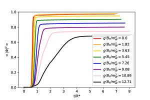
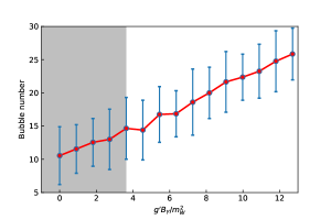
Figure 6: Top: Evolution of $\Phi^{2}$ over time under different non-helical homogeneous hyperMF strength. Bottom: The number of bubbles nucleated under different non-helical homogeneous hyperMF strengths. The gray area indicates the magnetic field strength where Higgs condensation has not yet occurred.

Fig. 6 shows the change of the Higgs field over time and the number of bubbles under different homogeneous non-helical hyperMF strengths. It can be seen that when the MF strength increases, the PT speed becomes slower and more bubbles are nucleated, which reflects that the strong MF affects the electroweak vacuum. When a bubble is nucleated, the strong MF acts rapidly on the true vacuum area inside the bubble. This not only reduces the vacuum expectation value of the Higgs field but also slows down the expansion speed of the bubble, causing the false vacuum to occupy the space of the universe for a longer period, which further results in the creation of more vacuum bubbles.

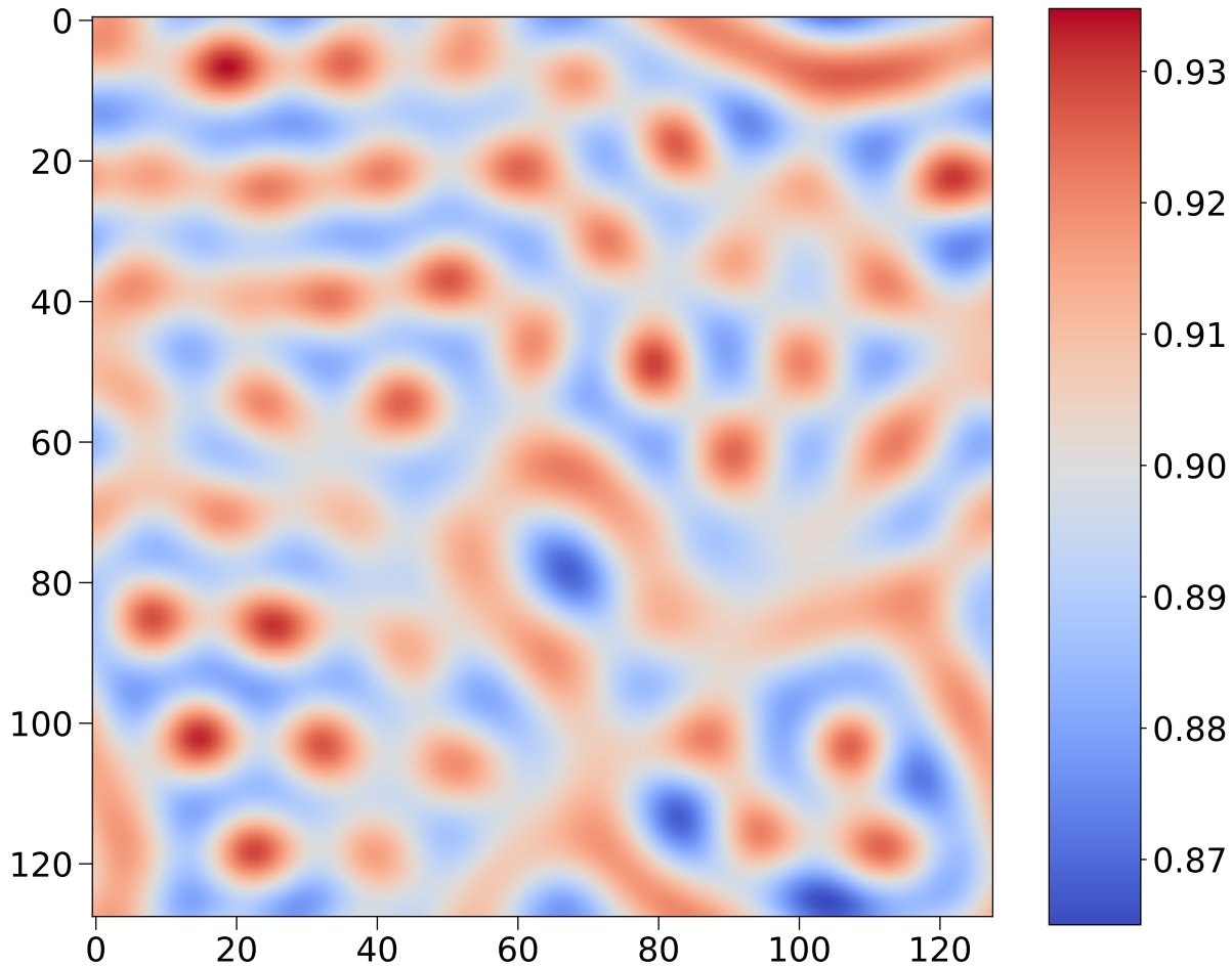
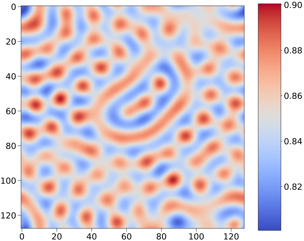
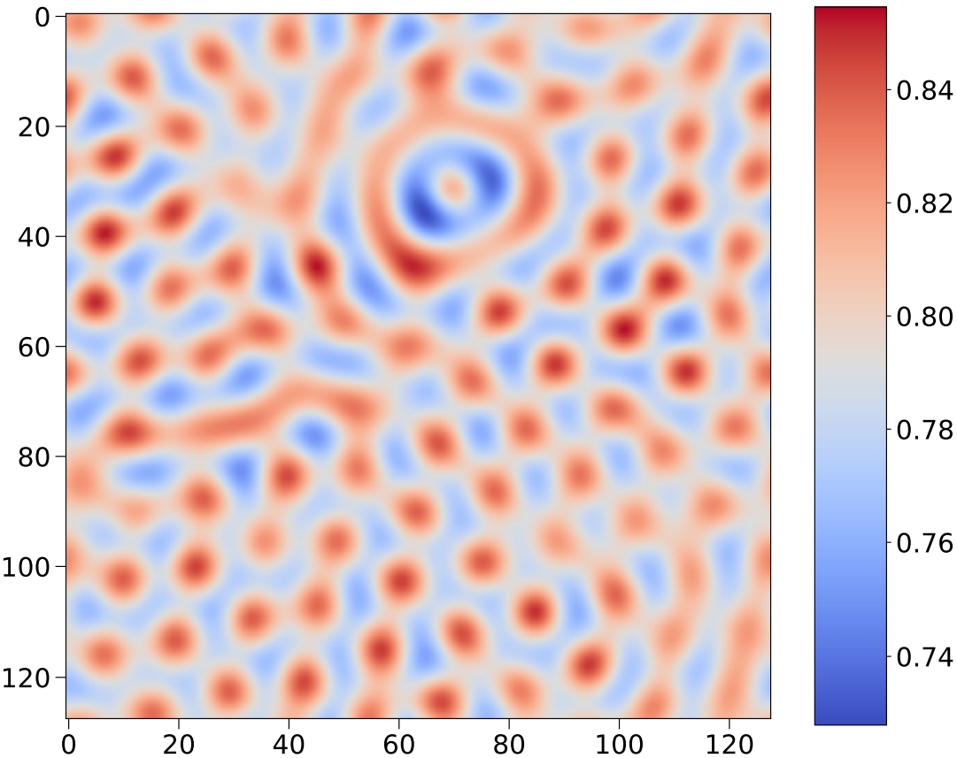
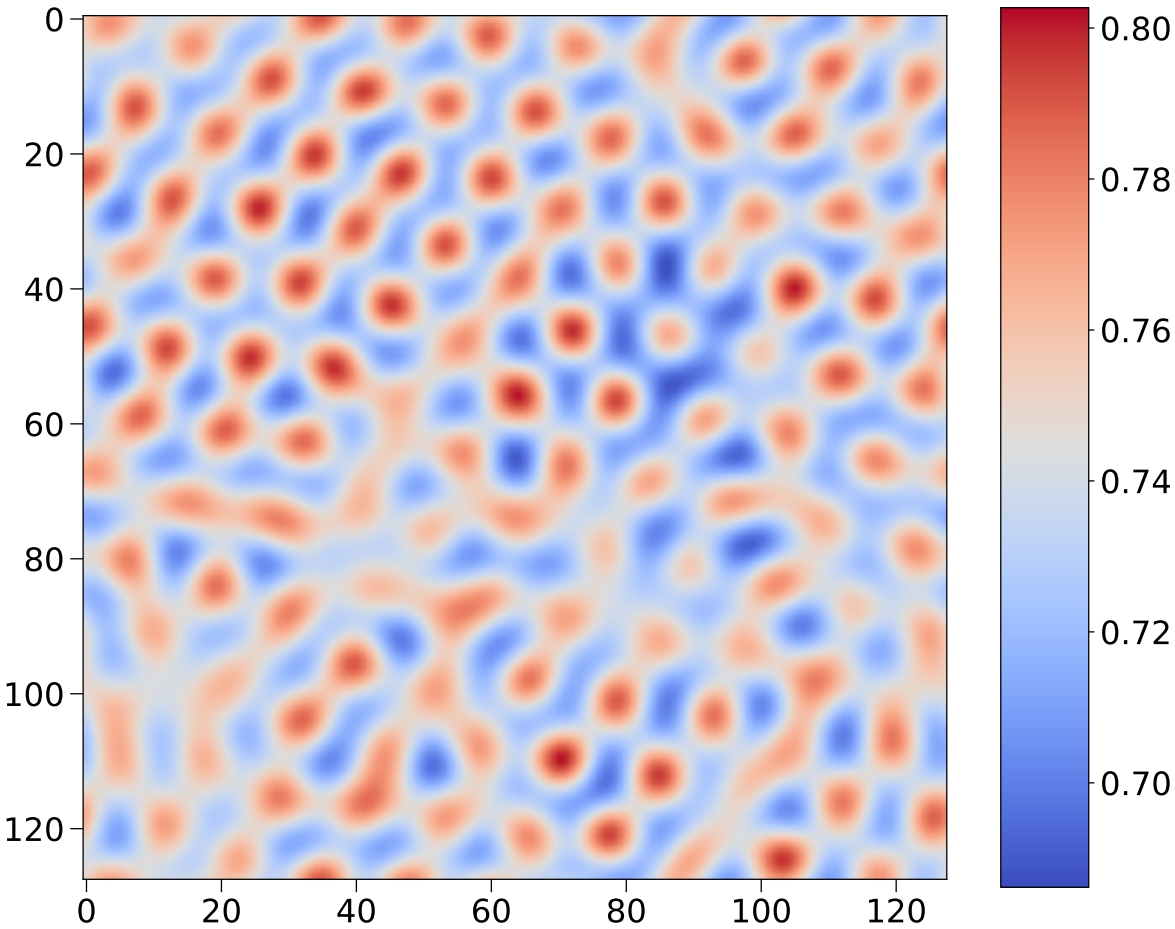
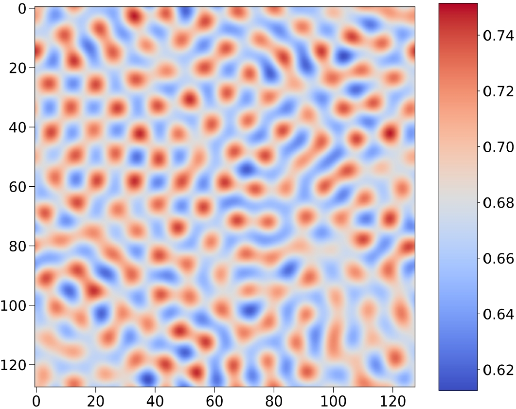
Figure 7: $\bar{\Phi}^{2}$ under different non-helical homogeneous hyperMFs. From left to right, from top to bottom, $g^{\prime}B_{Y}/m_{W}^{2}$ varies from $0$ to $12.71$ in intervals of $1.82$. As the MF increases, Higgs field gradually assumes a regular hexagonal vortex arrangement. When $g^{\prime}B_{Y}/m_{W}^{2}$ is approximately $3$, Higgs condensation begins to appear. The stronger the hyperMF, the denser the vortex.

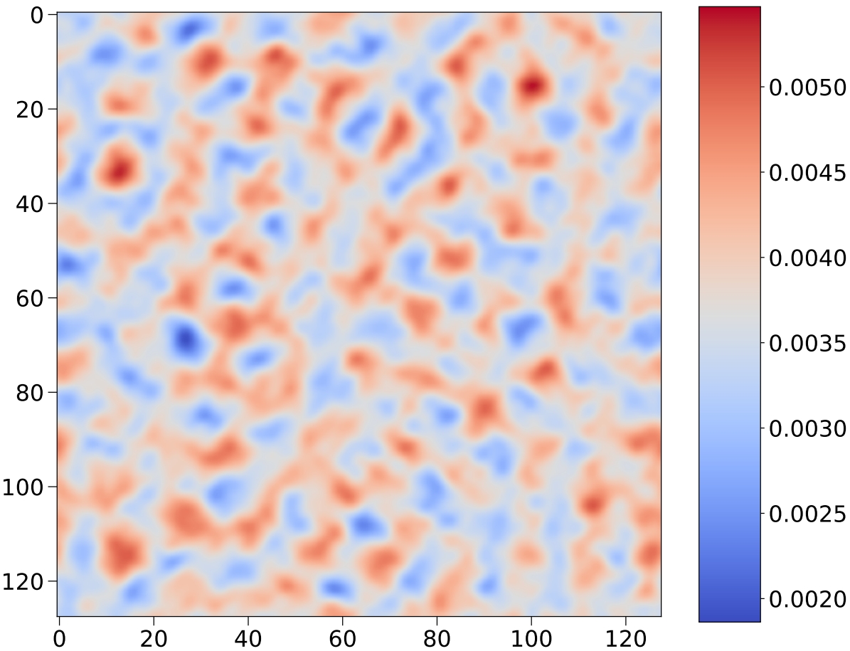
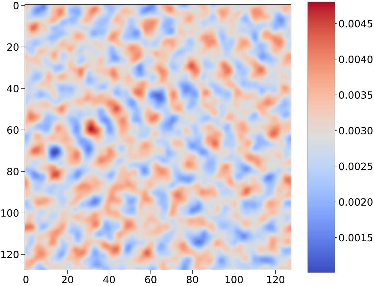
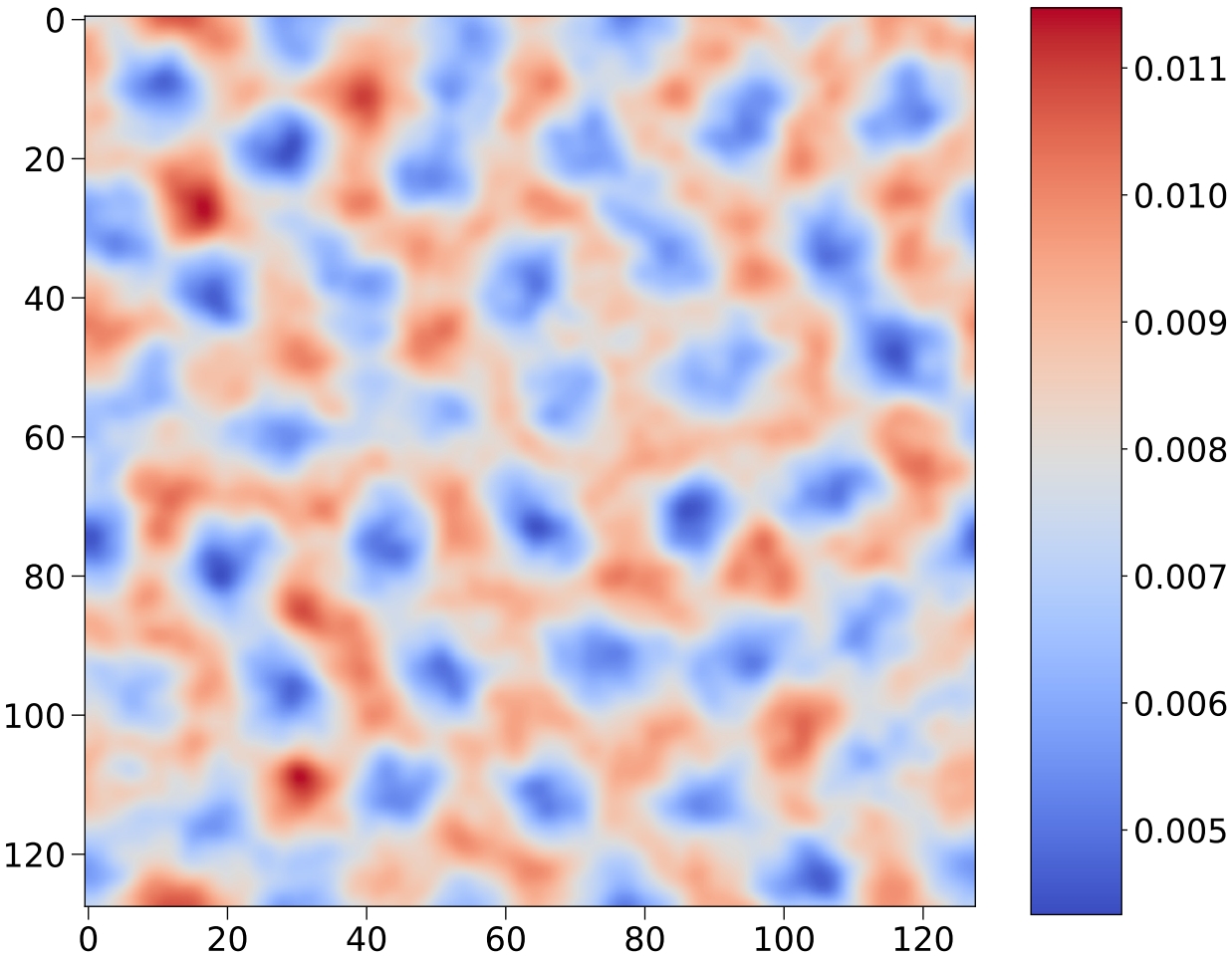
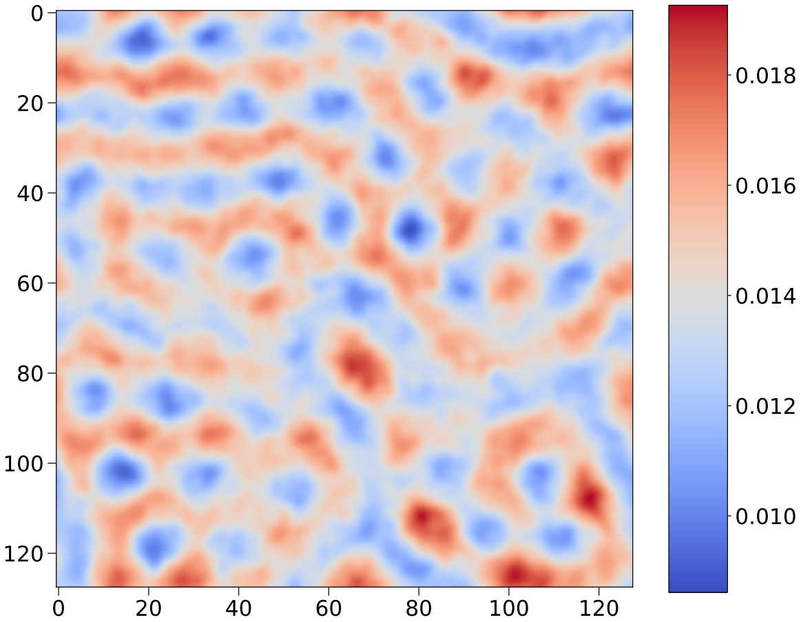
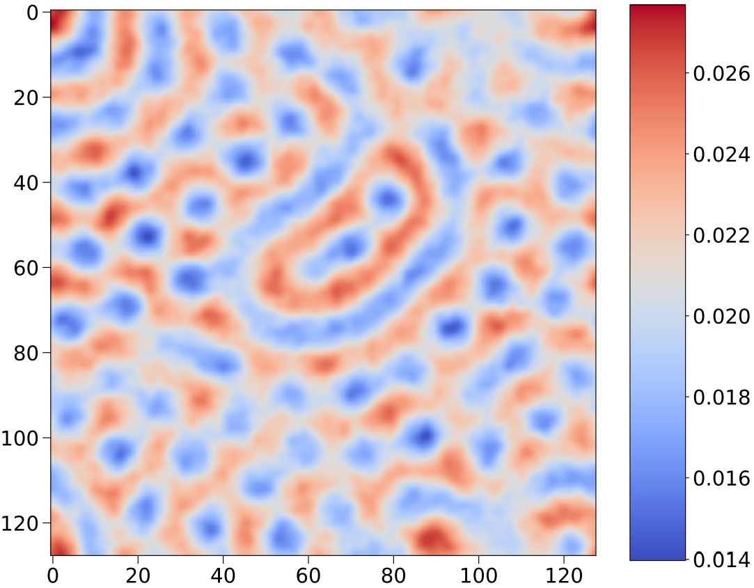
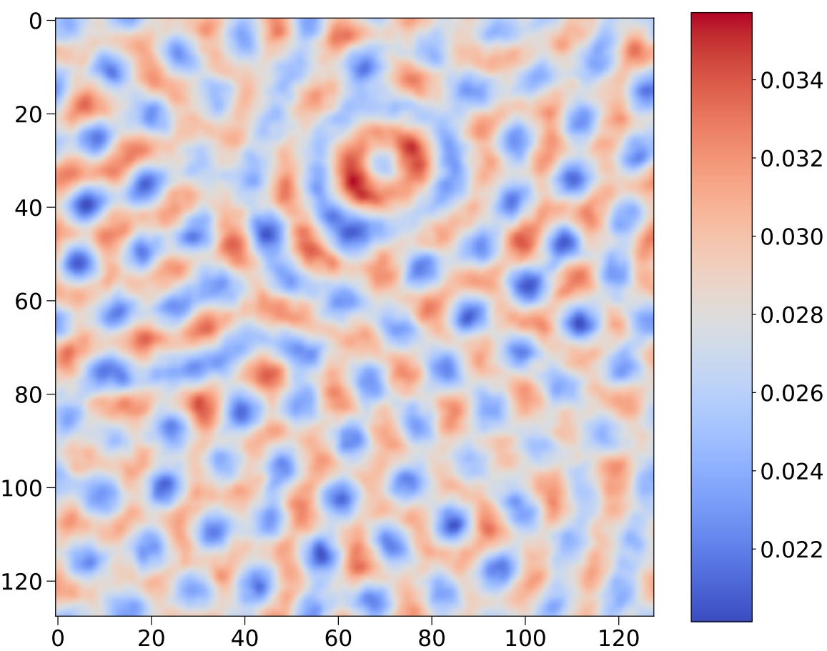
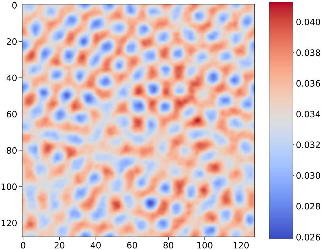
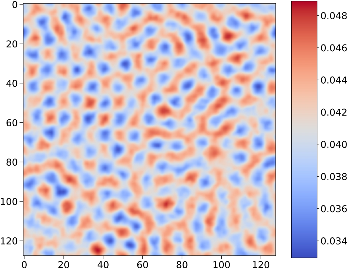
Figure 8: $\bar{W}_{\perp}$ under different non-helical homogeneous hyperMFs. From left to right, from top to bottom, $g^{\prime}B_{Y}/m_{W}^{2}$ varies from $0$ to $12.71$ in intervals of $1.82$. It is worth mentioning that every time step of the Higgs field is involved in the averaging, while $W$ field is only averaged every 100 steps, so the picture of $\bar{W}_{\perp}$ is rougher.

Fig. 7 and Fig. 8 show the changes of $\bar{\Phi}^{2}$ and $\bar{W}_{\perp}$ under different non-helical homogeneous hyperMFs. It can be seen that $\bar{W}_{\perp}$ vanishes at the center of the vortex, which is exactly the opposite of $\bar{\Phi}^{2}$. Moreover, as the hyperMF increases, the vortex becomes more and more dense.

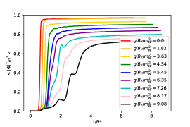
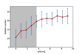
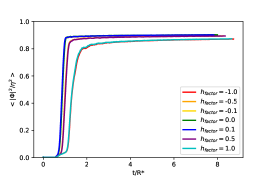
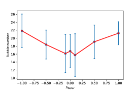
Figure 9: Left: Evolution of $\Phi^{2}$ over time under different helical homogeneous hyperMF strength with $h_{\mathrm{factor}}=1$ (Top) and under the same homogeneous hyperMF strength ($g^{\prime}B_{Y}/m_{W}^{2}=5.45$) and different $h_{\mathrm{factor}}$ (Bottom). Right: The number of bubbles nucleated under different MF strengths with $h_{\mathrm{factor}}=1$ (Top) and under different $h_{\mathrm{factor}}$ with homogeneous hyperMF strength being fixed at $g^{\prime}B_{Y}/m_{W}^{2}=5.45$ (Bottom). The gray area indicates the magnetic field strength where Higgs condensation has not yet occurred.

The effects of homogeneous helical hyperMF on the PT speed and the number of bubbles are similar to those without helicity. As shown in the top panels of Fig. 9, the helical homogeneous hyperMF makes the PT speed slower and also makes the final stable field value smaller. This shows that the speed of bubble expansion is slowed down in the hyperMF with helicity, and the bubble expansion speed is further reduced compared with the hyperMF without helicity.

The helicity will also slightly affect the PT process. As shown in the bottom panels in Fig. 9, as the initial helicity increases, the PT speed will decrease slightly, and the final value of $\Phi^{2}$ will also become smaller. This is just as we stated before, the speed at which the bubble expands is further slowed down by the helicity.

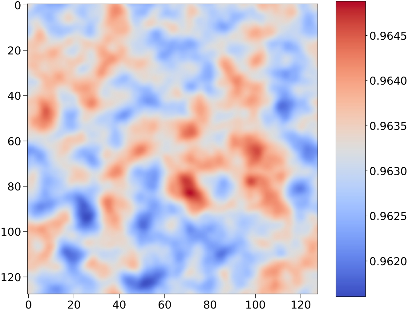
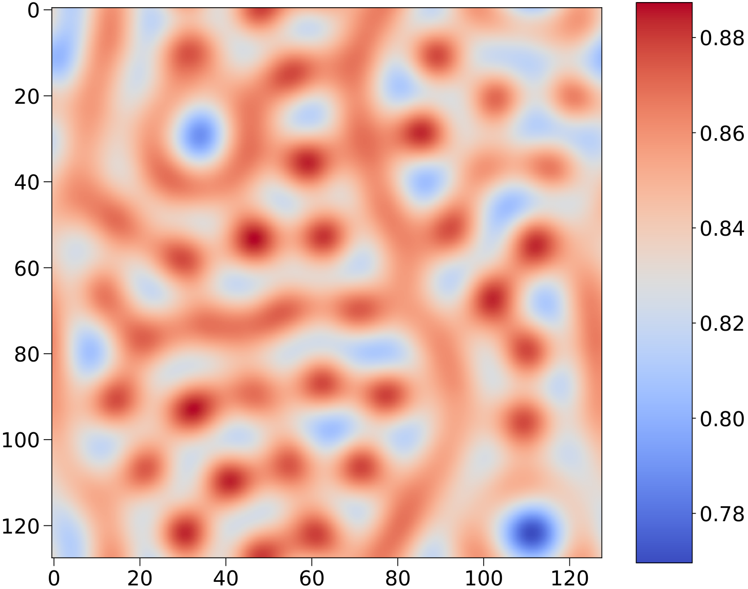
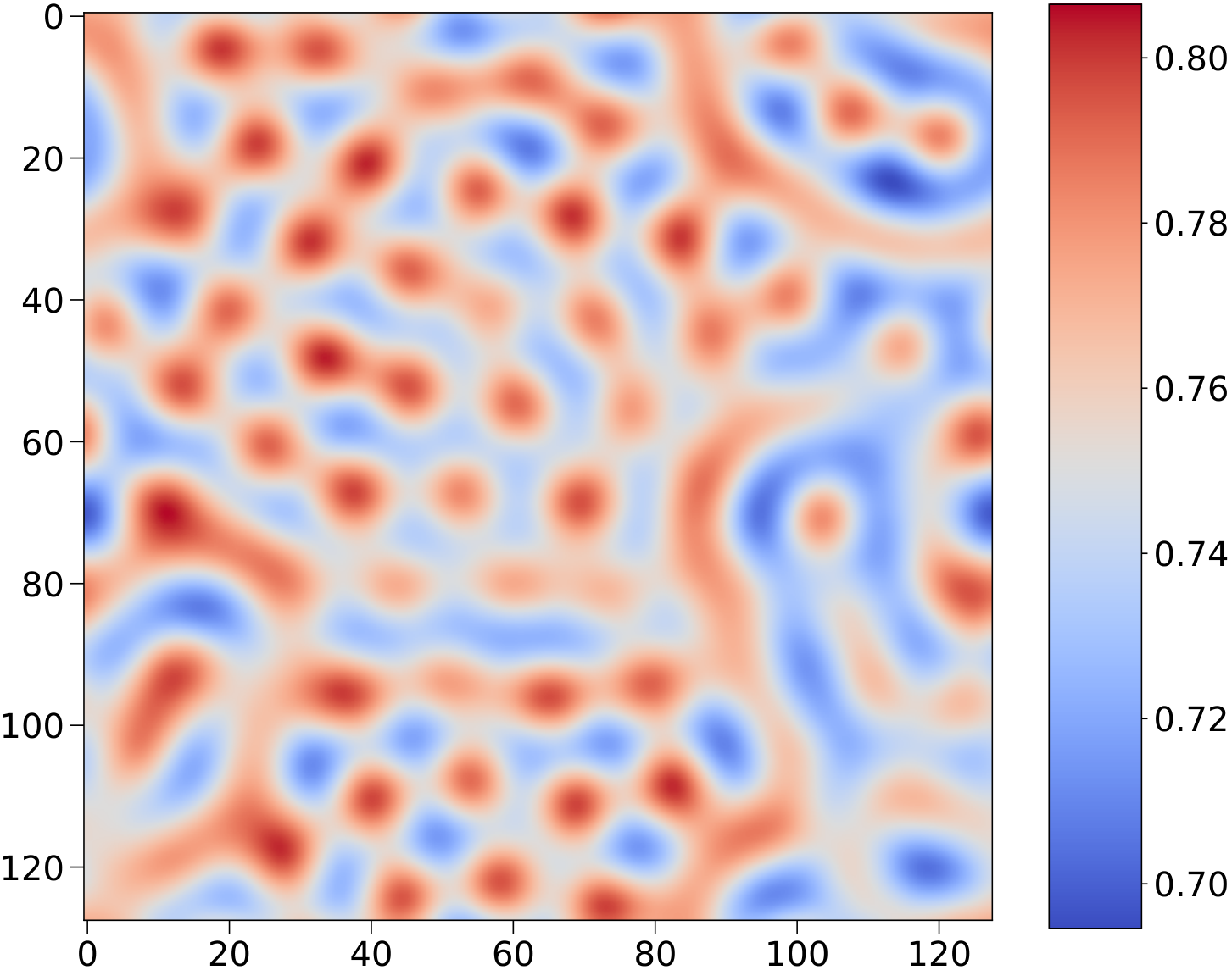
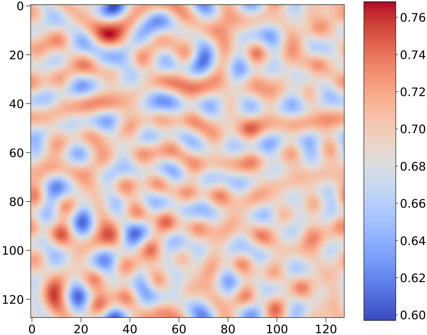
Figure 10: $\bar{\Phi}^{2}$ under different helical homogeneous MFs with $h_{\mathrm{factor}}=1$. From left to right, from top to bottom, $g^{\prime}B_{Y}/m_{W}^{2}$ varies from $1.82$ to $9.08$ in intervals of $1.82$. $\bar{\Phi}^{2}$ exhibits the same behavior as under a non-helical homogeneous hyperMF.

Fig. 10 shows the variation of $\bar{\Phi}^{2}$ with the strength of the homogeneous MF with helicity, and the behavior exhibited is similar to that in the non-helical MF. When $g^{\prime}B_{Y}/m^{2}_{W}>3.63$, the Higgs condensate phenomenon appears.

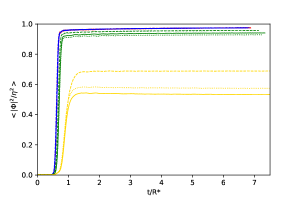
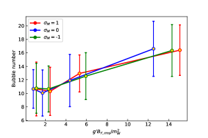
Figure 11: Left: Evolution of $\Phi^{2}$ over time under different spectrum index $n$ or different hyperMF with spectral distribution. The correspondence between color and $n$ is listed in table 1. The solid line indicates $\sigma_{\mathrm{M}}=1$, the dashed line indicates $\sigma_{\mathrm{M}}=-1$, and the dotted line indicates $\sigma_{\mathrm{M}}=0$, respectively. Right: The number of bubbles nucleated under different spectrum-distributed hyperMF strengths.

Unlike the previous cases, the PT speed did not decrease significantly due to the increase in spectrum-distributed hyperMF strength. This is because the PT has been completed quickly in the area with a smaller hyperMF as shown in the left panel of Fig. 11. The decrease in $\langle|\Phi|^{2}\rangle$ is because $\Phi$ has not undergone a PT in the area with a stronger MF and is still in the symmetric phase. What is the same as before is that the number of bubbles increases with the increase of the MF, as shown in the right panel of Fig. 11.

$n$	color	$\sigma_{\mathrm{M}}$	run times	$k_{\mathrm{UV}}$
$0$	yellow	$0,\ \pm 1$	$20$	$2\Delta k$
$1$	green
$2$	blue
$3$	red

Table 1: The parameters for spectrum distribution hyperMF situation. Color represents the different colors used for the lines in the left panel of Fig. 11 and Fig. 14. $\Delta k=2\pi/L$.

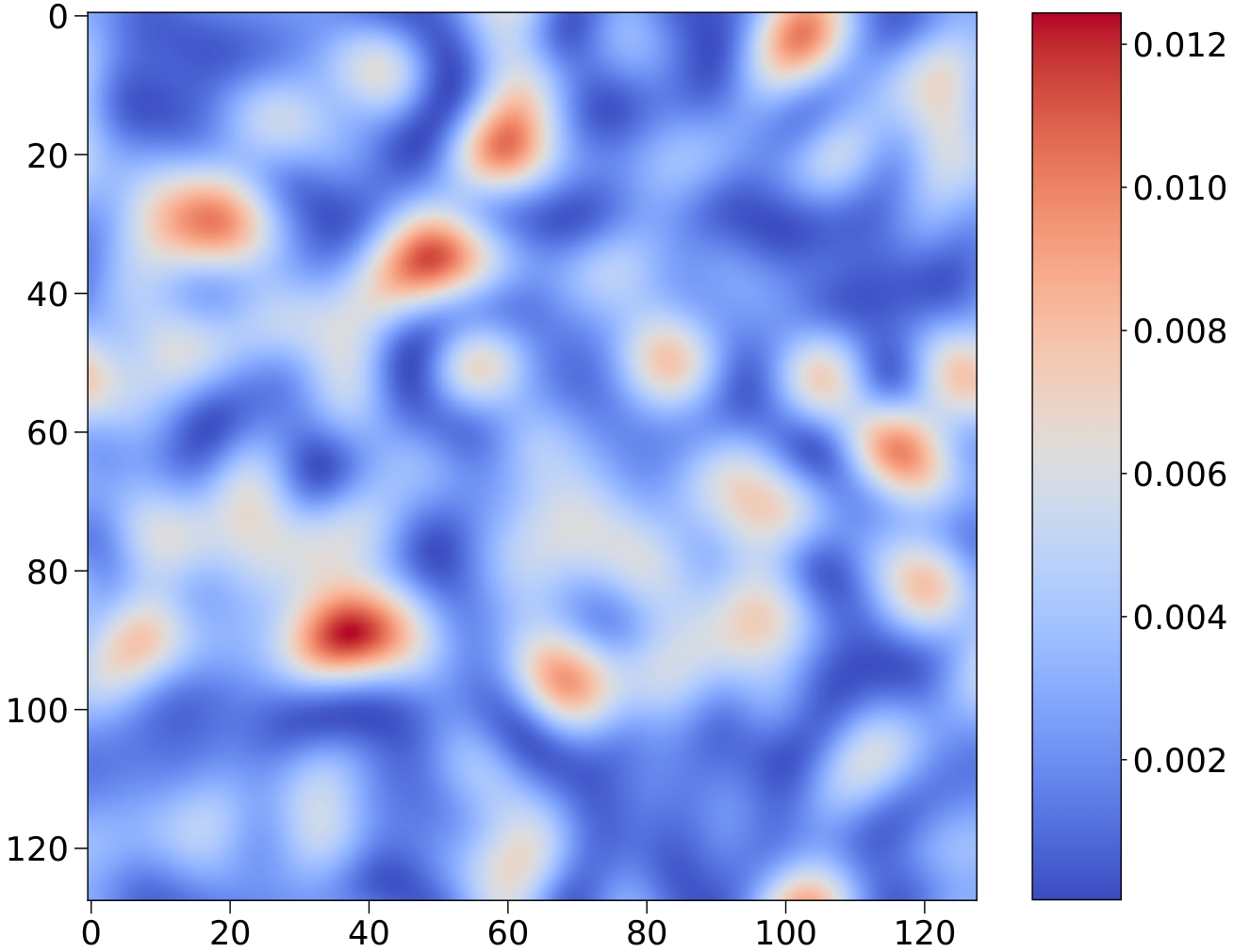
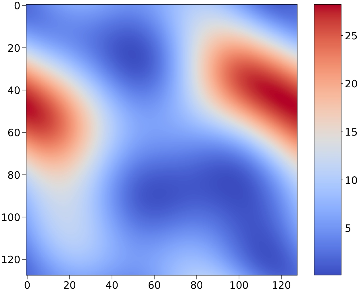
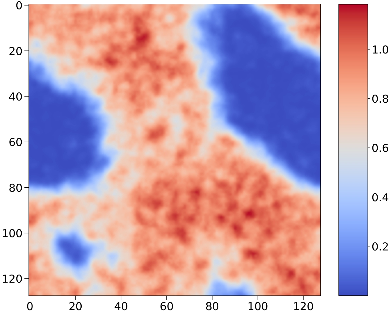
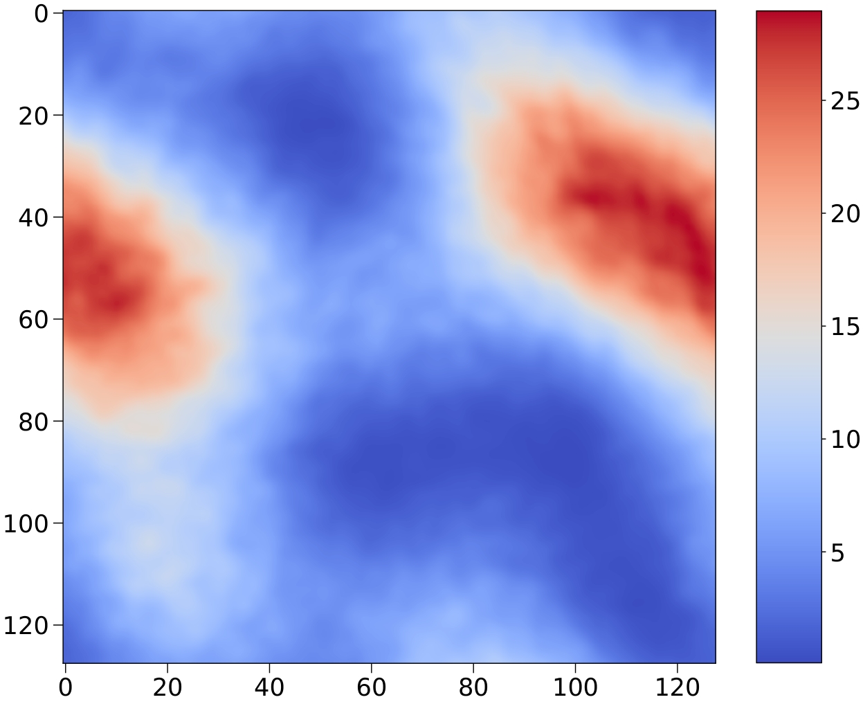
Figure 12: Top: Slice of $|\Phi|^{2}$(left) and hypermagnetic energy(right) at the beginning of the simulation. Bottom: Slice of $|\Phi|^{2}$(left) and hypermagnetic energy(right) at the end of the simulation. The hyperMF is a hyperMF with a spectral distribution.

Slices of $|\Phi|^{2}$ and hypermagnetic energy at the beginning and end of the simulation are shown in Fig. 12. It can be seen that at the beginning of the simulation, on the one hand, the hyperMF is no longer homogeneous in space, but with some places having high energy and some places being almost zero, on the other hand, $|\Phi|^{2}$ has thermal fluctuations according to (32). At the end of the simulation, because the background MF does not change with time, the distribution of hyperMF energy is similar to that at the beginning. However, it should be noted that $|\Phi|^{2}$ at the end tells us that the PT is only successfully and quickly completed in areas with small hyperMFs, while in places with large hyperMFs, $\Phi$ is still in the symmetric phase. Due to the random hyperMF distribution, unlike the homogeneous hyperMF with a fixed direction, the Higgs condensation phenomenon cannot be observed.

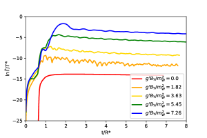
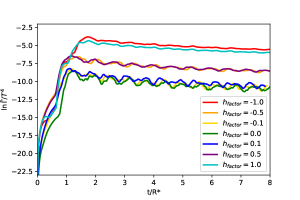
Figure 13: Left: Changes of $(\ln\,\bar{\Gamma}(t)/T^{4})$ over time under different homogeneous helical MFs with $h_{\mathrm{factor}}=1$. Right: Changes of $(\ln\,\bar{\Gamma}(t)/T^{4})$ over time at different initial helicity with homogeneous hyperMF fixed at $g^{\prime}B_{Y}/m_{W}^{2}=5.45$.

IX Electroweak Sphaleron During the Phase Transition under Hypermagnetic Field

Fig. 13 shows that the increase of hyperMF strength will significantly elevate $\bar{\Gamma}(t)$, that is, the rate of baryon production is faster. If the hyperMF is fixed and the helicity is increased, the rate of baryon production will also increase, but the effect is not as obvious as that brought by increasing the MF strength.

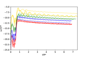
Figure 14: Evolution of $(\ln\,\bar{\Gamma}(t)/T^{4})$ over time under different index $n$ of the spectrum distributed hyperMF. The correspondence between color and $n$ is listed in table 1. The solid line indicates $\sigma_{\mathrm{M}}=1$, the dashed line indicates $\sigma_{\mathrm{M}}=-1$, and the dotted line indicates $\sigma_{\mathrm{M}}=0$, respectively.

The change of time-averaged sphaleron rate $\bar{\Gamma}$ with time under different spectral indices is shown in the top panel of Fig. 14, and the correspondence between color and spectral index or hyperMF energy density is shown in Table 1. It can be seen that $\ln\,\bar{\Gamma}/T^{4}$ with the same color represents the same spectral index and similar hyperMF strength. As the MF energy increases, the sphaleron rate also increases.

X Hypermagnetic Fields and Matter-Antimatter Asymmetry

We analyze the quantitative relationship between matter-antimatter asymmetry and hyperMF strength. From the simulation results, we can see that when the hyperMF with helicity is larger, $\eta_{\mathrm{B}}$ is also larger, and it has far exceeded the current observation result $\eta_{\mathrm{B}}\sim 10^{-10}$. Limited by the simulation conditions, we cannot simulate a smaller hyperMF, but using the fitting formula (12) and (14), we can infer the hyperMF strength required to achieve the correct $\eta_{\mathrm{B}}$.

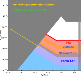
Figure 15: The yellow line and green line show the evolution of strength and correlation length of the spectral distribution MF and helical homogeneous MF that can achieve the correct baryon asymmetry, respectively. The gray region is excluded by MHD turbulent decay and CMB anisotropy measurements Durrer and Neronov (2013). The projected sensitivity of the Cherenkov Telescope Array observations to intergalactic MF strength is marked with red region Abdalla et al. (2021). Orange regions are excluded at the 95% to 99% confidence level from H.E.S.S. Abramowski et al. (2014), MAGIC Aleksic et al. (2010) and VERITAS Archambault et al. (2017). The dark and light blue regions are excluded by the lower bounds on IGMF strength from Fermi-LAT Taylor et al. (2011); Ackermann et al. (2018).

For a homogeneous (comoving) MF, the correlation length is infinite. Regardless of whether there is helicity or not, its evolution law follows $B_{\mathrm{rec}}/B_{\mathrm{EW}}=(\tau_{\mathrm{rec}}/\tau_{\mathrm{EW}})^{-5/7}$ Brandenburg et al. (2020b), where $\tau$ is conformal time, and the subscripts rec and EW represent the recombination epoch and electroweak PT epoch, respectively. In summary, the homogeneous helical MF that can obtain the correct baryon asymmetry is about $3.5\times 10^{-17}$ Gauss today. The evolution of its correlation length and strength is shown by the green line in Fig. 15.

For the MF with a spectral distribution of a smaller correlation scale, under fully helical conditions, its (comoving) correlation scale evolves according to $\lambda_{\mathrm{rec}}/\lambda_{\mathrm{EW}}=(\tau_{\mathrm{rec}}/\tau_{\mathrm{EW}})^{2/3}$ and the (comoving) MF intensity evolves according to $B_{\mathrm{rec}}/B_{\mathrm{EW}}=(\tau_{\mathrm{rec}}/\tau_{\mathrm{EW}})^{-1/3}$  Kahniashvili et al. (2016); Brandenburg et al. (2020b, 2021). The evolution of the MF that can obtain the correct baryon asymmetry is shown by the yellow line in Fig. 15. At present, the correlation length and strength of the MF reach $2.4\times 10^{-4}$ Mpc and $4.8\times 10^{-15}$ Gauss, respectively.

The above results do not conflict with current observations and theoretical calculations, so the first-order electroweak PT in the (hyper)MF background can indeed serve as a possible source of the origin of matter-antimatter asymmetry.

XI Chiral Potential and Lepton Asymmetry

The time evolution of $\Delta\mu$ is displayed in Fig. 16. When the PT occurs, $\Delta\mu$ increases suddenly, and then the fluctuation amplitude is stabilized. Moreover, the larger the initial helicity, the larger the amplitude, and the $h_{\mathrm{factor}}$ with opposite signs will bring completely opposite behaviors.

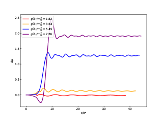
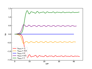
Figure 16: Left: The time evolution of the difference of left and right chemical potentials $\Delta\mu=\mu_{L}-\mu_{R}$ in homogeneous helical hyperMF background with $h_{\mathrm{factor}}=1$. Right: The time evolution of the difference of left and right chemical potentials $\Delta\mu=\mu_{L}-\mu_{R}$ under helical homogeneous hyperMF whose strength is fixed at $g^{\prime}B_{Y}/m_{W}^{2}=5.45$.

Fig. 17 shows the evolution of $\Delta\mu$ over time under spectral-distributed hyperMF. Again, when the PT occurs, the curve has a sharp rise and then oscillates. The curves of opposite helicity have opposite behaviors.

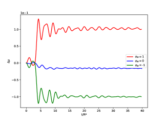
Figure 17: The time evolution of the difference of left and right chemical potentials $\Delta\mu=\mu_{L}-\mu_{R}$ under spectrally distributed hyperMF, which reflects the lepton asymmetry. The spectral index is fixed at $n=0$.

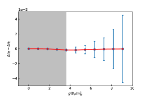
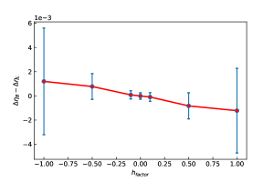
Figure 18: Left: Changes of $\eta_{\mathrm{B}}-\eta_{\mathrm{L}}$ under different homogeneous helical hyperMFs with $h_{\mathrm{factor}}=1$. The gray area indicates the magnetic field strength where Higgs condensation has not yet occurred. Right: Changes of $\eta_{\mathrm{B}}-\eta_{\mathrm{L}}$ at different initial helicity with homogeneous hyperMF fixed at $g^{\prime}B_{Y}/m_{W}^{2}=5.45$.

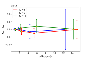
Figure 19: $\eta_{\mathrm{B}}-\eta_{\mathrm{L}}$ under different spectrum distributed hyperMF strength with $n=0$.

We also checked the B$-$L symmetry, and the variations of $\eta_{\mathrm{B}}-\eta_{\mathrm{L}}$ in a helical homogeneous hyperMF and a spectrally distributed hyperMF are shown in Fig. 18 and Fig. 19, respectively. It can be seen that under different hyperMFs or helicity, $\eta_{\mathrm{B}}-\eta_{\mathrm{L}}\sim 0$, indicating that the B$-$L symmetry is well tested.

References

- Wielebinski (2005) R. Wielebinski, “Magnetic fields in the milky way, derived from radio continuum observations and faraday rotation studies,” in Cosmic Magnetic Fields, edited by R. Wielebinski and R. Beck (Springer Berlin Heidelberg, Berlin, Heidelberg, 2005) pp. 89–112.
- Clarke et al. (2001) T. E. Clarke, P. P. Kronberg, and H. Böhringer, The Astrophysical Journal 547, L111–L114 (2001).
- Bonafede et al. (2010) A. Bonafede, L. Feretti, M. Murgia, F. Govoni, G. Giovannini, D. Dallacasa, K. Dolag, and G. B. Taylor, Astronomy and Astrophysics 513, A30 (2010).
- Feretti et al. (2012) L. Feretti, G. Giovannini, F. Govoni, and M. Murgia, The Astronomy and Astrophysics Review 20 (2012), 10.1007/s00159-012-0054-z.
- Dolag et al. (2010) K. Dolag, M. Kachelriess, S. Ostapchenko, and R. Tomàs, The Astrophysical Journal 727, L4 (2010).
- Tavecchio et al. (2010) F. Tavecchio, G. Ghisellini, L. Foschini, G. Bonnoli, G. Ghirlanda, and P. Coppi, Monthly Notices of the Royal Astronomical Society: Letters 406, L70–L74 (2010).
- Tavecchio et al. (2011) F. Tavecchio, G. Ghisellini, G. Bonnoli, and L. Foschini, Monthly Notices of the Royal Astronomical Society 414, 3566–3576 (2011).
- Vovk et al. (2012) I. Vovk, A. M. Taylor, D. Semikoz, and A. Neronov, The Astrophysical Journal 747, L14 (2012).
- Hogan (1983) C. J. Hogan, Phys. Rev. Lett. 51, 1488 (1983).
- Di et al. (2021) Y. Di, J. Wang, R. Zhou, L. Bian, R.-G. Cai, and J. Liu, Physical Review Letters 126 (2021), 10.1103/physrevlett.126.251102.
- Enqvist and Olesen (1993) K. Enqvist and P. Olesen, Phys. Lett. B 319, 178 (1993), arXiv:hep-ph/9308270 .
- Yang and Bian (2022) J. Yang and L. Bian, Physical Review D 106 (2022), 10.1103/physrevd.106.023510.
- Vachaspati (1991) T. Vachaspati, Phys. Lett. B 265, 258 (1991).
- Baym et al. (1996) G. Baym, D. Bodeker, and L. D. McLerran, Phys. Rev. D 53, 662 (1996), arXiv:hep-ph/9507429 .
- Grasso and Riotto (1998) D. Grasso and A. Riotto, Phys. Lett. B 418, 258 (1998), arXiv:hep-ph/9707265 .
- Quashnock et al. (1989) J. M. Quashnock, A. Loeb, and D. N. Spergel, Astrophys. J. Lett. 344, L49 (1989).
- Turner and Widrow (1988) M. S. Turner and L. M. Widrow, Phys. Rev. D 37, 2743 (1988).
- Adshead et al. (2016) P. Adshead, J. T. Giblin, T. R. Scully, and E. I. Sfakianakis, JCAP 10, 039 (2016), arXiv:1606.08474 [astro-ph.CO] .
- Martin and Yokoyama (2008) J. Martin and J. Yokoyama, JCAP 01, 025 (2008), arXiv:0711.4307 [astro-ph] .
- Kanno et al. (2009) S. Kanno, J. Soda, and M.-a. Watanabe, JCAP 12, 009 (2009), arXiv:0908.3509 [astro-ph.CO] .
- Ratra (1992) B. Ratra, Astrophys. J. Lett. 391, L1 (1992).
- Grasso and Rubinstein (2001) D. Grasso and H. R. Rubinstein, Physics Reports 348, 163–266 (2001).
- Widrow (2002) L. M. Widrow, Reviews of Modern Physics 74, 775–823 (2002).
- Kulsrud and Zweibel (2008) R. M. Kulsrud and E. G. Zweibel, Reports on Progress in Physics 71, 046901 (2008).
- Kandus et al. (2011) A. Kandus, K. E. Kunze, and C. G. Tsagas, Physics Reports 505, 1–58 (2011).
- Widrow et al. (2011) L. M. Widrow, D. Ryu, D. R. G. Schleicher, K. Subramanian, C. G. Tsagas, and R. A. Treumann, Space Science Reviews 166, 37–70 (2011).
- Durrer and Neronov (2013) R. Durrer and A. Neronov, The Astronomy and Astrophysics Review 21 (2013), 10.1007/s00159-013-0062-7.
- Dermer et al. (2011) C. D. Dermer, M. Cavadini, S. Razzaque, J. D. Finke, J. Chiang, and B. Lott, The Astrophysical Journal 733, L21 (2011).
- Taylor et al. (2011) A. M. Taylor, I. Vovk, and A. Neronov, Astronomy amp; Astrophysics 529, A144 (2011).
- Neronov and Vovk (2010) A. Neronov and I. Vovk, Science 328, 73–75 (2010).
- Nielsen and Olesen (1978) N. K. Nielsen and P. Olesen, Nucl. Phys. B 144, 376 (1978).
- MacDowell and Törnkvist (1992) S. W. MacDowell and O. Törnkvist, Phys. Rev. D 45, 3833 (1992).
- Salam and Strathdee (1975) A. Salam and J. Strathdee, Nuclear Physics B 90, 203 (1975).
- Linde (1976) A. Linde, Physics Letters B 62, 435 (1976).
- Ambjørn (1989) J. Ambjørn, Physics Letters B: Particle Physics, Nuclear Physics and Cosmology 220, 659 (1989).
- Chernodub et al. (2023) M. Chernodub, V. Goy, and A. Molochkov, Physical Review Letters 130 (2023), 10.1103/physrevlett.130.111802.
- Giovannini and Shaposhnikov (1998a) M. Giovannini and M. E. Shaposhnikov, Physical Review Letters 80, 22–25 (1998a).
- Giovannini and Shaposhnikov (1998b) M. Giovannini and M. E. Shaposhnikov, Phys. Rev. D 57, 2186 (1998b), arXiv:hep-ph/9710234 .
- Joyce and Shaposhnikov (1997) M. Joyce and M. E. Shaposhnikov, Phys. Rev. Lett. 79, 1193 (1997), arXiv:astro-ph/9703005 .
- Hindmarsh et al. (2021) M. Hindmarsh, M. Lüben, J. Lumma, and M. Pauly, SciPost Physics Lecture Notes (2021), 10.21468/scipostphyslectnotes.24.
- Caldwell et al. (2022) R. Caldwell, Y. Cui, H.-K. Guo, V. Mandic, A. Mariotti, J. M. No, M. J. Ramsey-Musolf, M. Sakellariadou, K. Sinha, L.-T. Wang, G. White, Y. Zhao, H. An, L. Bian, C. Caprini, S. Clesse, J. M. Cline, G. Cusin, B. Fornal, R. Jinno, B. Laurent, N. Levi, K.-F. Lyu, M. Martinez, A. L. Miller, D. Redigolo, C. Scarlata, A. Sevrin, B. S. E. Haghi, J. Shu, X. Siemens, D. A. Steer, R. Sundrum, C. Tamarit, D. J. Weir, K.-P. Xie, F.-W. Yang, and S. Zhou, General Relativity and Gravitation 54 (2022), 10.1007/s10714-022-03027-x.
- Athron et al. (2024) P. Athron, C. Balázs, A. Fowlie, L. Morris, and L. Wu, Progress in Particle and Nuclear Physics 135, 104094 (2024).
- Morrissey and Ramsey-Musolf (2012) D. E. Morrissey and M. J. Ramsey-Musolf, New Journal of Physics 14, 125003 (2012).
- Cohen et al. (2012) T. Cohen, D. E. Morrissey, and A. Pierce, Physical Review D 86 (2012), 10.1103/physrevd.86.013009.
- Mazumdar and White (2019) A. Mazumdar and G. White, Reports on Progress in Physics 82, 076901 (2019).
- Caprini et al. (2016) C. Caprini, M. Hindmarsh, S. Huber, T. Konstandin, J. Kozaczuk, G. Nardini, J. M. No, A. Petiteau, P. Schwaller, G. Servant, and D. J. Weir, Journal of Cosmology and Astroparticle Physics 2016, 001–001 (2016).
- Caprini et al. (2020) C. Caprini, M. Chala, G. C. Dorsch, M. Hindmarsh, S. J. Huber, T. Konstandin, J. Kozaczuk, G. Nardini, J. M. No, K. Rummukainen, P. Schwaller, G. Servant, A. Tranberg, and D. J. Weir, Journal of Cosmology and Astroparticle Physics 2020, 024–024 (2020).
- Amaro-Seoane et al. (2017) P. Amaro-Seoane et al. (LISA), (2017), arXiv:1702.00786 [astro-ph.IM] .
- Luo et al. (2016) J. Luo, L.-S. Chen, H.-Z. Duan, Y.-G. Gong, S. Hu, J. Ji, Q. Liu, J. Mei, V. Milyukov, M. Sazhin, C.-G. Shao, V. T. Toth, H.-B. Tu, Y. Wang, Y. Wang, H.-C. Yeh, M.-S. Zhan, Y. Zhang, V. Zharov, and Z.-B. Zhou, Classical and Quantum Gravity 33, 035010 (2016).
- Ruan et al. (2020) W.-H. Ruan, Z.-K. Guo, R.-G. Cai, and Y.-Z. Zhang, International Journal of Modern Physics A 35, 2050075 (2020), https://doi.org/10.1142/S0217751X2050075X .
- Guada et al. (2020) V. Guada, M. Nemevšek, and M. Pintar, Computer Physics Communications 256, 107480 (2020).
- Brandenburg et al. (2020a) A. Brandenburg, R. Durrer, Y. Huang, T. Kahniashvili, S. Mandal, and S. Mukohyama, Physical Review D 102 (2020a), 10.1103/physrevd.102.023536.
- Adler (1969) S. L. Adler, Phys. Rev. 177, 2426 (1969).
- Bell and Jackiw (1969) J. S. Bell and R. Jackiw, Nuovo Cim. A 60, 47 (1969).
- ’t Hooft (1976a) G. ’t Hooft, Phys. Rev. Lett. 37, 8 (1976a).
- ’t Hooft (1976b) G. ’t Hooft, Phys. Rev. D 14, 3432 (1976b), [Erratum: Phys.Rev.D 18, 2199 (1978)].
- Moore (2002) G. D. Moore, Physical Review D (2002), 10.1103/physrevd.59.014503.
- Tranberg and Smit (2003) A. Tranberg and J. Smit, JHEP 11, 016 (2003), arXiv:hep-ph/0310342 .
- Annala and Rummukainen (2023) J. Annala and K. Rummukainen, Phys. Rev. D 107, 073006 (2023).
- Boyarsky et al. (2012) A. Boyarsky, J. Fröhlich, and O. Ruchayskiy, Phys. Rev. Lett. 108, 031301 (2012).
- Bali et al. (2012) G. S. Bali, F. Bruckmann, G. Endrődi, Z. Fodor, S. D. Katz, S. Krieg, A. Schäfer, and K. K. Szabó, Journal of High Energy Physics (2012), 10.1007/jhep02(2012)044.
- Abdalla et al. (2021) H. Abdalla et al. (CTA), JCAP 02, 048 (2021), arXiv:2010.01349 [astro-ph.HE] .
- Abramowski et al. (2014) A. Abramowski et al. (H.E.S.S.), Astron. Astrophys. 562, A145 (2014), arXiv:1401.2915 [astro-ph.HE] .
- Aleksic et al. (2010) J. Aleksic et al. (MAGIC), Astron. Astrophys. 524, A77 (2010), arXiv:1004.1093 [astro-ph.HE] .
- Archambault et al. (2017) S. Archambault et al. (VERITAS), Astrophys. J. 835, 288 (2017), arXiv:1701.00372 [astro-ph.HE] .
- Ackermann et al. (2018) M. Ackermann et al. (Fermi-LAT), Astrophys. J. Suppl. 237, 32 (2018), arXiv:1804.08035 [astro-ph.HE] .
- Brandenburg et al. (2020b) A. Brandenburg, R. Durrer, Y. Huang, T. Kahniashvili, S. Mandal, and S. Mukohyama, Physical Review D (2020b), 10.1103/physrevd.102.023536.
- Kahniashvili et al. (2016) T. Kahniashvili, A. Brandenburg, and A. G. Tevzadze, Physica Scripta , 104008 (2016).
- Brandenburg et al. (2021) A. Brandenburg, Y. He, and R. Sharma, arXiv: Cosmology and Nongalactic Astrophysics,arXiv: Cosmology and Nongalactic Astrophysics (2021).