Branching brownian motion conditioned on large level sets

Abstract.

We study the precise large deviation probabilities for the sizes of intermediate level sets in branching Brownian motion (BBM). Our conclusions improve on a result of Aïdekon, Hu and Shi in [J. Math. Sci. 238(2019)]. Additionally, we analyze the typical behaviors of BBM conditioned on large level sets. Our approach relies on the connections between intermediate level sets, additive martingale limits of BBM, and the global minimum of linearly transformed BBMs.

1. Introduction

We consider a standard binary branching Brownian motion (BBM) on the real line, which is a particle system constructed inductively as follows. Initially, a single particle performs standard Brownian motion. After an exponentially distributed random time with mean one that is independent of its motion, the particle undergoes a branching event: it dies and produces two offspring at its current position. Each offspring then independently continues the same process, performing Brownian motion and eventually branching in the same manner. We denote by $\mathcal{N}_{t}$ the sets of all particles alive at time $t$ and by $X_{t}(u)$ the position of $u\in\mathcal{N}_{t}$.

To characterize how this cloud of particles is distributed in space, one of the most fundamental aspects is to determine the sizes of the level sets, defined as follows. For each $y\geq 0$, the $y$-level set of the BBM at time $t$ consists of all particles alive at time $t$ that are positioned above the level $y$. Let $\mathscr{L}_{t}(y)$ denote the size of the $y$-level set:

$$\mathscr{L}_{t}(y):=\#\{u\in\mathcal{N}_{t}:X_{t}(u)\geq y\}.$$ (1.1)

For $x\geq 0$, the typical asymptotic behavior of the sizes of $xt$-level sets is well understood:

Almost surely, for sufficiently large time $t$, the $\sqrt{2}t$-level set at large time $t$ is empty, while $\mathscr{L}_{t}(xt)$ is comparable to its expectation for each $x\in[0,\sqrt{2})$.

Precisely, it was proved by Hu and Shi [HS09] for branching random walks (BRWs) and Robert [Rob13] for BBMs that the maximal position $M_{t}:=\max_{u\in\mathcal{N}_{t}}X_{t}(u)$ satisfies

$$\limsup_{t\to\infty}\frac{\sqrt{2}t-M_{t}}{\log t}=\frac{3}{2\sqrt{2}}\text{ a.s. \, and }\,\liminf_{t\to\infty}\frac{\sqrt{2}t-M_{t}}{\log t}=\frac{1}{2\sqrt{2}}\text{ a.s. }$$ (1.2)

This implies the emptiness of $\sqrt{2}t$-level set. Additionally, Biggins [Big79] for BRWs and Glenz, Kistler, Schmidt for BBMs [GKS18] showed that

$$\frac{\mathscr{L}_{t}(xt)}{\mathbf{E}\left[\mathscr{L}_{t}(xt)\right]}\xrightarrow{t\to\infty}W_{\infty}(x):=\lim_{t\rightarrow\infty}\sum_{u\in\mathcal{N}_{t}}e^{xX_{t}(u)-\left(1+\frac{x^{2}}{2}\right)t}\ \text{ a.s.}$$ (1.3)

Additionally, Biggins [Big92] described the distribution of the BBM around the level $xt$, showing that $\sum_{u\in\mathcal{N}_{t}}\frac{f(X_{t}(u)-xt)}{\mathbf{E}\left[\mathscr{L}_{t}(xt)\right]}\overset{t\to\infty}{\rightarrow}W_{\infty}(x)\int f(h)e^{-xh}\mathop{}\!\mathrm{d}h$ for any continuous function $f$ of compact support and $x\in[0,\sqrt{2})$.

Once the typical behavior is understood, one may be interested in exploring the atypical behavior of the level sets. Aïdekon, Hu and Shi [AHS19] investigated the upper deviation probability of the level sets, examining both BBMs and the Gaussian free field (GFF). They demonstrated that for $x>0$ and $(1-\frac{x^{2}}{2})_{+}<a<1$, the following holds:

$$\lim_{t\to\infty}\frac{1}{t}\ln\mathbf{P}\left(\mathscr{L}_{t}(xt)\geq e^{at}\right)=-I(x,a),$$ (1.4)

where the rate function $I(\cdot,\cdot)$ is defined by

$$I(x,a):=\frac{x^{2}}{2(1-a)}-1.$$ (1.5)

In other words, $\mathbf{P}\left(\mathscr{L}_{t}(xt)\geq e^{at}\right)=e^{-I(x,a)t+o(t)}$. This $o(t)$ term hides important information about the evolution of the BBM conditioned on the level set being large. For example, [AHS19, §3.1] showed that the strategy $\max_{u\in\mathcal{N}_{pt}}X_{pt}(u)\geq bpt$ (where $p$ and $b$ are defined in (1.6)) can induce this atypical event. However, determining whether this strategy is optimal (i.e., whether this is a typical event for the conditioned process), hinges on the precise order of the $o(t)$ term. Here comes our first question:

Question 1: What is the exact order of $\mathbf{P}\left(\mathscr{L}_{t}(xt)\geq e^{at}\right)$?

As highlighted above, our primary interest lies in understanding the typical behavior of the BBM when the level set is unusually large. For instance, what is the genealogy structure of these particles above level $xt$ conditioned on $\mathscr{L}_{t}(xt)\geq e^{at}$? What is the distribution of the maximal position $\max_{u\in\mathcal{N}_{t}}X_{t}(u)$ conditioned on $\mathscr{L}_{t}(xt)\geq e^{at}$? Overall, our second question read as follows:

Question 2: What is the typical behavior of the BBM under $\mathbf{P}\left(\cdot\mid\mathscr{L}_{t}(xt)\geq e^{at}\right)$?

1.1. Main results

Our first main result Theorem 1.1 solves Question 1. We first introduce three important parameters that appear everywhere in this paper:

$$\theta:=\frac{2(1-a)}{x},\ p:=\frac{(1-a)\left[x^{2}-2(1-a)\right]}{x^{2}-2(1-a)^{2}},\text{ and }\ b:=\frac{2}{\theta}=\frac{x}{1-a}.$$ (1.6)

We emphasis that $\theta\in(0,\sqrt{2})$ and $p\in(0,1-a)$ for any $x>0$ and $(1-\frac{x^{2}}{2})_{+}<a<1$. Moreover, for any $|\lambda|<\sqrt{2}$, define

$$C_{W_{\infty}(\lambda)}:=\lim_{y\to\infty}y^{\frac{2}{\lambda^{2}}}\mathbf{P}\left(W_{\infty}(\lambda)>y\right).$$ (1.7)

The fact that $C_{W_{\infty}(\lambda)}\in(0,\infty)$ for $|\lambda|<\sqrt{2}$ is obtained in [Liu00], with a different proof also provided in [CdRM24].

Theorem 1.1 (Precise Large Deviation Estimates).

Fix $x>0$, $(1-\frac{x^{2}}{2})_{+}<a<1$, and $y>0$. We have

$$\mathbf{P}\left(\mathscr{L}_{t}(xt)\geq\frac{y}{\sqrt{t}}e^{at}\right)=[1+o(1)]\hyperref@@ii[eq-cst-a-x]{C_{\star}}(x,a)y^{-\frac{2}{\theta^{2}}}e^{-I(x,a)t}\text{ as }t\to\infty.$$ (1.8)

Above, the constant $\hyperref@@ii[eq-cst-a-x]{C_{\star}}(\cdot,\cdot)$ is defined by

$$\hyperref@@ii[eq-cst-a-x]{C_{\star}}(x,a):=\frac{C_{W_{\infty}(\theta)}}{(\theta\sqrt{2\pi(1-p)})^{\frac{2}{\theta^{2}}}}.$$ (1.9)

Our first theorem slightly differs from Question 1, which asks about the decay rate of $\mathbf{P}(L_{t}(xt)\geq e^{at})$, simply because we found it more convenient to present the result (and its proof) for $\mathbf{P}(L_{t}(xt)\geq e^{at}/\sqrt{t})$. The reason is that the law of large numbers (1.3) suggests it is more natural to consider the large deviation probability of $L_{t}(xt)/\mathbf{E}[L_{t}(xt)]$, and there do have a $t^{-1/2}$ term in $\mathbf{E}[L_{t}(xt)]$. Nonetheless, an immediate adaptation of our method provides the answer for the original form of Question 1: For any fixed $y>0$,

$$\mathbf{P}\left(\mathscr{L}_{t}(xt)\geq ye^{at}\right)\sim C_{\hyperref@@ii[eq-cst-a-x]{\star}}(x,a)y^{-\frac{2}{\theta^{2}}}t^{-\frac{1}{\theta^{2}}}e^{-I(x,a)t}\ \text{ as }t\to\infty.$$ (1.10)

Here is an immediate corollary of our first theorem. Recall that a random variable $X$ is said to have the Pareto distribution with parameter $\lambda>0$, if $\mathbf{P}(X>y)=y^{-\lambda}$ for $y\geq 1$ and $\lambda>0$. Then Theorem 1.1 yields that

$$\left(\sqrt{t}e^{-at}\mathscr{L}_{t}(xt)\mid\mathscr{L}_{t}(xt)\geq e^{at}/\sqrt{t}\right)\text{ converges in law to }\mathrm{Pareto}\left({2}/{\theta^{2}}\right).$$ (1.11)

This provides a partial answer to Question 2 concerning the behavior of the level set when conditioned on it being large. In theorems 1.2 and 1.3, we examine the conditional distribution of two particularly interesting quantities in the BBM: the overlap and the maximal position, respectively. Before presenting our results, we introduce some essential terminology. For any two particles $u,v\in\cup_{r\geq 0}\mathcal{N}_{r}$, the overlap between $u$ and $v$ is defined as the covariance of their positions, conditionally on the genealogy structure of the BBM:

$$\mathscr{R}(u,v) :=\mathbf{E}\left[X(u)X(v)\mid\mathcal{N}_{r},r\geq 0\right]$$ (1.12)

$$=\text{ the death time of the most recent common ancestor of }u\text{ and }v.$$ (1.13)

For a given $t>0$, we introduce a crucial curve in studying the level set large deviation probability, as noted by [AHS19]. Let

$$\mathsf{F}_{t}(r):=t\,\mathsf{f}\left(\frac{r}{t}\right),\,r\in[0,t],\text{ where }\mathsf{f}(\lambda):=x-\mathbf{1}_{\left\{a+\lambda\leq 1\right\}}\sqrt{2(1-\lambda)(1-\lambda-a)}.$$ (1.14)

Theorem 1.2 (Entropy Repulsion: Overlap).

Given $x>0$ and $(1-\frac{x^{2}}{2})_{+}<a<1$. Conditioned on the BBM up to time $t$, select two particles $u^{1}_{t},u^{2}_{t}$ independently and uniformly from the $xt$-level set. Define

$$\mathfrak{s}:=\operatorname*{arg\,min}_{t>0}\min_{v\in\mathcal{N}_{t}}\left\{\left(\frac{\theta^{2}}{2}+1\right)t-\theta X_{t}(v)\right\}.$$ (1.15)

Then the collection of random vectors, conditionally on a large level set size,

$$\left(\mathscr{R}(u^{1}_{t},u^{2}_{t})-\mathfrak{s},X_{\mathscr{R}(u^{1}_{t},u^{2}_{t})}(u_{t}^{1})-\mathsf{F}_{t}(\mathscr{R}(u^{1}_{t},u^{2}_{t}))\mid\mathscr{L}_{t}(xt)\geq\frac{e^{at}}{\sqrt{t}}\right)_{t>0}\text{ is tight }.$$ (1.16)

As a consequence, we have the following conditional central limit theorem:

$$\left(\frac{\mathscr{R}(u^{1}_{t},u^{2}_{t})-pt}{\sqrt{pt}},\frac{X_{\mathscr{R}(u^{1}_{t},u^{2}_{t})}(u^{1}_{t})-bpt}{\sqrt{pt}}\mid\mathscr{L}_{t}(xt)\geq\frac{e^{at}}{\sqrt{t}}\right)\Rightarrow G\left(\frac{\theta}{1-\theta^{2}/2},\frac{1+\theta^{2}/2}{1-\theta^{2}/2}\right),$$ (1.17)

where $G$ is a standard Gaussian random variable.

Recall that $M_{t}:=\max_{u\in\mathcal{N}_{t}}X_{t}(u)$ denotes the maximal position of the particles in the BBM at time $t$.

Theorem 1.3 (Entropy Repulsion: Maximum).

Given $x>0$ and $(1-\frac{x^{2}}{2})_{+}<a<1$. Let $v:=bp+\sqrt{2}(1-p)$. Then as $t\to\infty$,

$$\left(\frac{M_{t}-vt}{\sqrt{t}}\mid\mathscr{L}_{t}(xt)\geq\frac{e^{at}}{\sqrt{t}}\right)\Rightarrow\frac{\sqrt{2}-\theta}{\sqrt{2}+\theta}\,G,$$ (1.18)

where $G$ is a standard Gaussian random variable.

Remark 1.4.

In contrast to Theorems 1.2 and 1.3, without conditioning, the overlap converges in distribution, and the maximal position exhibits a ballistic spreading speed $\sqrt{2}<v$. More precisely, we will prove in Lemma 2.5 that

$$\lim_{t\to\infty}\mathbf{P}(\mathscr{R}(u^{1}_{t},u^{2}_{t})\geq r)=\mathbf{E}\left[\sum_{v\in\mathcal{N}_{r}}\left(e^{xX_{r}(v)-(\frac{x^{2}}{2}+1)r}\frac{W_{\infty}^{(v)}(x)}{W_{\infty}(x)}\right)^{2}\right],\,\forall\,r>0.$$ (1.19)

And the limiting distribution has no mass at infinity: $\lim\limits_{r\to\infty}\lim\limits_{t\to\infty}\mathbf{P}(\mathscr{R}(u^{1}_{t},u^{2}_{t})\geq r)=0$. Additionally, it is well-known that $M_{t}$ satisfies (see for example [Bra83, Aïd13, BDZ16])

$$M_{t}-\sqrt{2}t+\frac{3}{2\sqrt{2}}\log t\text{ converges in law.}$$ (1.20)

We regard Theorems 1.2 and 1.3 as phenomena of entropy repulsion: the imposed constraint that $\mathscr{L}_{t}(xt)\geq e^{at}/\sqrt{t}$ alters the natural evolution of the BBM, compelling a particle in the BBM to reach the space-time curve $(r,F_{t}(r))$ at some random time $r$ around $pt$, with Gaussian fluctuations of order $\sqrt{t}$.

Remark 1.5.

Although in this paper, ocus on the simplest binary branching Brownian motion setting, as in [AHS19], our approach could be applied to the context of the branching random walk under the same framework as in [CdRM24].

1.2. Related work and further questions

In this paper, we focus exclusively on rare events where the level sets become unusually large. The lower deviation probabilities, where the level set is unusually small, were investigated in [Öz20] for BBMs and [Zha23] for BRWs, with the corresponding rate functions obtained. It is also interesting to study BRWs on $\mathbb{R}^{d}$ or on general graphs. We refer to [AB14] for BRWs on $\mathbb{R}^{d}$ and to [LMW24] for BRWs on free groups, where the exponential growth rate of the level sets was obtained. Additionally, branching random walks are closely connected to random recursive tree (and random search trees), see [Dev87, Pit94, ABF13]. In particular, by using the result on the minimum of BRWs, [ABF13] showed that the height of a random recursive tree on $n$ nodes is $e\ln n-\frac{3}{2}\ln(\ln n)+O_{\mathbf{P}}(1)$. A natural question arising from this is whether the results on level sets of BRWs can be extended to describe the growth rate of the number of nodes at a distance greater than $\lambda e\ln n$, with $\lambda\in(0,1)$.

In [GKS18], Glenz, Kistler, and Schmidt conjectured that a law of large numbers, as stated in (1.3), holds for all models within the BBM-universality class (see [Zei12, Kis14, Arg16, BK22]). Biskup and Louidor confirmed this for intermediate level sets of the two-dimensional discrete Gaussian free field (2D DGFF) in [BL19]. The large deviation probabilities for these level sets in the 2D DGFF were studied by Aïdékon, Hu, and Shi in [AHS19]. While the rate function was derived, a precise estimate similar to Theorem 1.1, remains unclear. Furthermore, results similar to (1.3) have been shown for local times of two-dimensional random walks in [AB22], for the local times of planar Brownian motion in [Jeg20], and for a random model of the Riemann-zeta function in [AHK22]. However, the large deviation probabilities for these models are still not fully understood, and we believe they are worth further exploration.

1.3. Proof ideas

First let us recall the arguments in [AHS19]. If we start the BBM at time-space point $(r,\mathsf{F}_{t}(r))$, under what conditions will there be approximately $e^{at+o(t)}$ particles positioned above level $xt$ at time $t$ with positive probability? According to the law of large numbers (1.3), we need

$$(t-r)-\frac{[xt-\mathsf{F}_{t}(r)]^{2}}{2(t-r)}=at,\text{ if }r\leq(1-a),\text{ and }\mathsf{F}_{t}(r)=xt,\text{ if }r\geq(1-a)t.$$ (1.21)

This is exactly the definition (1.14). Thus, in order that $\{\mathscr{L}_{t}(xt)\geq e^{at}\}$ occurs, we need at time $r$ for there to be a particle positioned above level $\mathsf{F}_{t}(r)$. Since $\mathbf{P}(M_{r}\geq y)\approx e^{(1-\frac{y^{2}}{2})r+o(r)}$ for $y\geq\sqrt{2}r$, we choose the best choice of $r$ such that $\sup_{r\leq t}\left\{r-\frac{\mathsf{F}_{t}(r)^{2}}{2r}\right\}$ is attained. It turns out that the maximizer is $r^{*}=pt$, and

$$\sup_{r\leq(1-a)t}\left\{r-\frac{\mathsf{F}_{t}(r)^{2}}{2r}\right\}=-I(a,x).$$ (1.22)

This strategy gives the lower bound $\mathbf{P}(\mathscr{L}_{t}(xt)\geq e^{at})\geq e^{-I(x,a)t+o(t)}$ in [AHS19]. The corresponding upper bound, however, is more subtle. In [AHS19], the authors discretize space and time to classify possible trajectories, and estimate the number of particles following each one. Since the total number of trajectories grows sub-exponentially—specifically $\exp\{O(t^{1-\delta}\ln t)\}$—it appears challenging to improve their argument to obtain a tighter bound. However it is shown in [AHS19] that the probability of having more than $e^{at}$ particles following a trajectory that is far from $r\mapsto\mathsf{F}_{t}(r)$ is negligible compared to $e^{-I(a,t)t+o(t)}$. This lead us to guess that the optimal strategy for the large deviation event involves forcing the BBM approach the curve $r\mapsto\mathsf{F}_{t}(r)$ near the time $pt$.

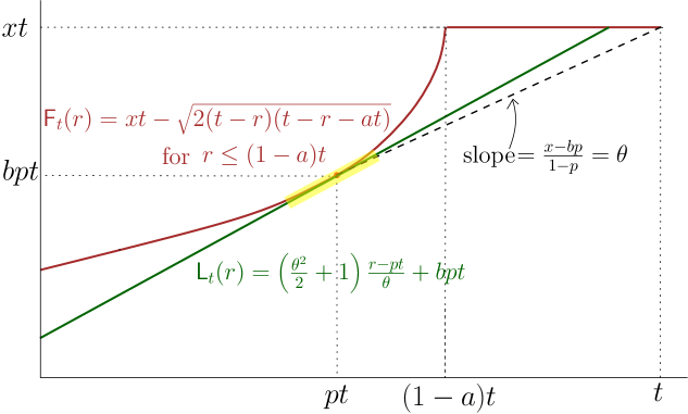
Figure 1. The functions $\mathsf{F}_{t}$ and $\mathsf{L}_{t}$

Studying the probability of BBM hitting a curve is challenging, while hitting a line is simpler. Our approach is to approximate $\mathsf{F}_{t}$ using its tangent line at the point $(pt,F_{t}(pt))$. Since $\mathsf{F}_{t}(pt)=bpt$, let $\mathsf{L}_{t}$ denote this tangent line at $(pt,bpt)$, see Figure 1. Then

$$\mathsf{L}_{t}(r):=\left(\frac{\theta^{2}}{2}+1\right)\frac{r-pt}{\theta}+bpt\quad\text{ for }r\in[0,t]$$ (1.23)

Observe that the BBM hits the line $\mathsf{L}_{t}$ if and only if there exists $r>0$ and $u\in\mathcal{N}_{r}$ such that $X_{r}(u)=\left(\frac{\theta^{2}}{2}+1\right)\frac{r-pt}{\theta}+bpt$. We define

$$V_{r}(u):=\left(\frac{\theta^{2}}{2}+1\right)r-\theta X_{r}(u)\ \text{ for all }u\in\mathcal{N}_{r},r\geq 0.$$ (1.24)

Since $b=2/\theta$, we can rewrite $X_{r}(u)=\left(\frac{\theta^{2}}{2}+1\right)\frac{r-pt}{\theta}+bpt$ as $V_{r}(u)=-(1-\frac{\theta^{2}}{2})pt$. Set

$$\mathbf{I}:=\min\{V_{t}(u):u\in\mathcal{N}_{r},r\geq 0\}.$$ (1.25)

Thus, the event that the BBM hits the line $\mathsf{L}_{t}$ is equivalent to the event that the global minimum $\mathbf{I}$ of the linearly transformed BBM is smaller than $-(1-\theta^{2}/2)pt$:

$$\{\text{BBM hits }\mathsf{L}_{t}\}=\left\{\mathbf{I}\leq-(1-\frac{\theta^{2}}{2})pt\right\}.$$ (1.26)

In §3 Proposition 3.1, we demonstrate that the probability of the event $\mathscr{L}_{t}(xt)\geq e^{at}/\sqrt{t}$ while $|\mathbf{I}+(1-\frac{\theta^{2}}{2})pt|>z$ is bounded above by $Ce^{-I(a,x)t-z/2}$. And in §4 we show that for fixed $z$, the probability of the event $\mathscr{L}_{t}(xt)\geq e^{at}/\sqrt{t}$ while $\mathbf{I}+(1-\frac{\theta^{2}}{2})pt\in[z,z+1]$ is asymptotically equivalent to $C_{z}e^{-I(a,x)t}$. This implies that (1.26) provides the optimal strategy for the large deviation event $\mathscr{L}_{t}(xt)\geq e^{at}/\sqrt{t}$.

The main challenge in this paper lies in proving Proposition 3.1, which is tackled using the following two key elements: (i) In Lemma 3.2 we provides a tighter upper bound for the large deviation probability than [AHS19] by use of the tail inequality for the martingale limit $W_{\infty}(\theta)$. (ii) A useful but seemingly overlooked inequality (Lemma 2.6) from [HN04] turns out can be combined with the moment estimate (2.8) obtained recently in [CdRM24] and Lemma 3.2 to conclude the desired result. In §4, we apply the widely-used spine decomposition technique along with the results from [CdRM24] on BRW conditioned on an extremely negative global minimum. This approach enables us to prove Theorems 1.1, 1.2, and 1.3.

Notation convention

Through our the paper, we assume $x>0$ and $(1-\frac{x^{2}}{2})_{+}<a<1$. The parameters $\theta,p,b$ are functions of $x,a$ as defined in (1.6). We denote $s:=pt$. Let $\psi=\psi_{\theta}$ represent the log-Laplace transform associated with $(V_{t}(u):u\in\mathcal{N}_{t})$: $\psi(\lambda):=\ln\mathbf{E}\left[\sum_{u\in\mathcal{N}_{1}}e^{-\lambda V_{1}(u)}\right]=\left(\frac{\theta^{2}}{2}\lambda-1\right)\left(\lambda-1\right)$ for $\lambda\in\mathbb{R}$. Let $\kappa$ be the largest zero of $\psi$. Then

$$\kappa=2/\theta^{2},\ \psi^{\prime}(\kappa)=1-{\theta^{2}}/{2}\text{ and }\psi^{\prime\prime}(\kappa)=\theta^{2}.$$ (1.27)

We can then rewrite the event in (1.26) as $\{\mathbf{I}\leq-\psi^{\prime}(\kappa)s\}$.

We use $C$ and $c$ to denote positive constants that may vary between lines. When a constant depends on a parameter $\lambda$, we write $C_{\lambda}$ or $c_{\lambda}$. We write $f\lesssim g$ to indicate that there exists a constant $C>0$ such that $f\leq Cg$, and $f\lesssim_{\lambda}g$ when the constant $C$ depends on $\lambda$. Additionally, we use the standard notation $\Theta(f)$ to denote a non-negative quantity such that $c_{1}f\leq\Theta(f)\leq c_{2}f$ for some constants $c_{1},c_{2}>0$.

2. Preliminaries

2.1. Spine Decomposition

The spinal decomposition is a powerful technique introduced in [LPP95] for studying Galton-Waston processes and generalized to BRWs and BBMs in [Lyo97, Kyp04]. Here we follow [Ber14, Chapter 4]. We will distinguish one particular line of descent from the root, so at each time there will be a marked particle that we will call the spine. By enlarging the probability space to take this extra information into account, we can significantly simplify the description of the process constructed via the probability titling using the additive martingale $(W_{t}(\beta))_{t\geq 0}$ defined by

$$W_{t}(\beta):=\sum_{u\in\mathcal{N}_{t}}e^{\beta X_{t}(u)-(\frac{\beta^{2}}{2}+1)t}$$ (2.1)

First, sample a standard BBM $(X_{t}(u):u\in\mathcal{N}_{t})$ according to $\mathbf{P}$. Conditioned on this BBM, we construct a distinguished line of descent from the root inductively as follows. Let $u_{0}$ denote the root particle in the BBM. For $j\geq 0$, select a child $u_{j+1}$ of $u_{j}$ uniformly at random. For each particle $u$, denote its death time by $d_{u}$ and its life time by $\eta_{v}$, respectively. Define $w_{t}=u_{j}$ for $t\in[d_{u_{j}}-\eta_{u_{j}},d_{u_{j}})$. (Note that $d_{u_{j+1}}=\eta_{u_{j+1}}+d_{u_{j}}$, so $w_{t}$ is well-defined for all $t\geq 0$.) Let $\mathbb{P}^{*}$ denote the law of the pair $(\{X_{t}(u):u\in\mathcal{N}_{t}\},w_{t})_{t\geq 0}$. Write $\Xi_{t}:=X_{t}(w_{t})$ for the position of the spine at time $t$. Let $(s_{j})_{j\geq 1}$ be the times of branching events along the spine, and $n=(n_{t})_{t\geq 0}$ be the corresponding counting process. (In other words $n_{t}=|w_{t}|$, where $|u|$ represents the generation of particle $u$). Then we have

$$\mathop{}\!\mathrm{d}\mathbf{P}^{*}(X,w)=\mathop{}\!\mathrm{d}\mathbb{W}(\Xi)\mathop{}\!\mathrm{d}\mathbb{L}(n)\prod_{j\geq 1}\frac{1}{2}\mathop{}\!\mathrm{d}\mathbf{P}_{\Xi(s_{j})}(X^{(j)}).$$ (2.2)

Above, $\mathbb{W}$ represents the Wiener measure, $\mathbb{L}$ represents the law of Poisson process with rate $1$, $\mathbf{P}_{x}$ is the law of standard BBM starting from $x$, and $X^{(j)}$ denotes the process $\{X_{s_{j}+t}(u)-\Xi(s_{j}):u\in\mathcal{N}^{(v_{j})}_{t}:t\geq 0\}$, where $v_{j}$ is the brother of $w_{s_{j}}$.

Let $(\mathcal{F}_{t})_{t\geq 0}$ and $(\mathcal{F}_{t}^{*})_{t\geq 0}$ denote the natural filtration of the BBM without and with a spine, respectively. Then it is clear that $(e^{\beta\Xi_{t}-{\beta^{2}t}/{2}}e^{-t}2^{n_{t}},\mathcal{F}^{*}_{t})_{t\geq 0}$ is a $\mathbf{P}^{*}$ martingale. Fix a bound stopping time $\tau$ of $(\mathcal{F}^{*}_{t})_{t\geq 0}$, we define the probability measure $(\mathbf{Q}^{\beta,*}_{\tau}\otimes\mathbf{P})$ by

$$\mathop{}\!\mathrm{d}(\mathbf{Q}^{\beta,*}_{\tau}\otimes\mathbf{P})(X,w):=e^{\beta\Xi_{\tau}-(\frac{\beta^{2}}{2}+1)\tau}2^{|w_{\tau}|}\mathop{}\!\mathrm{d}\mathbf{P}^{*}(X,w)$$ (2.3)

$$=e^{\beta\Xi_{\tau}-\frac{\beta^{2}}{2}\tau}\mathop{}\!\mathrm{d}\mathbb{W}(\Xi)e^{-\tau}2^{n_{\tau}}\mathop{}\!\mathrm{d}\mathbb{L}(n)\prod_{j\geq 1}\frac{1}{2}\mathop{}\!\mathrm{d}\mathbf{P}_{\Xi(s_{j})}(X^{(j)}).$$ (2.4)

The construction in (2.4) shows that the process under $\mathbf{Q}^{\beta,*}_{\tau}\otimes\mathbf{P}$ corresponds to the law of a non-homogeneous branching motion with distinguished and randomized spine having the following properties:

• Spine particles behave differently from the ordinary particles before the stopping time $\tau$: They perform a Brownian motion with drift $\beta$ and branch according to their own (independent) exponential clocks with rate $2$. But after the stopping time $\tau$, spine particles follow the same dynamics as the ordinary particles.

• At each branching event of a spine particle, one of its two offspring is chosen uniformly at random to continue as the new spine particle, while the other becomes an ordinary particle.

• Ordinary particles initiate $\mathbf{P}$-BBMs at their space-time point of creation.

Lemma 2.1.

The spinal decomposition can be stated as follows.

1. Under $\mathbf{Q}^{\beta,*}_{\tau}\otimes\mathbf{P}$, $\left(\Xi_{t}-\beta(t\wedge\tau):t\geq 0\right)$ is a standard Brownian motion.

2. Assume that $\tau$ is a bounded stopping time w.r.t. $(\mathcal{F}_{t})$. Then

   $$\mathop{}\!\mathrm{d}(\mathbf{Q}^{\beta,{*}}_{\tau}\otimes\mathbf{P})|_{\mathcal{F}_{\infty}}=W_{\tau}(\beta)\mathop{}\!\mathrm{d}\mathbf{P}.$$ (2.5)

   Moreover, for any particle $u$,

   $$(\mathbf{Q}^{\beta,{*}}_{\tau}\otimes\mathbf{P})(w_{\tau}=u\mid\mathcal{F}_{\infty})=\frac{1}{W_{\tau}(\beta)}\,e^{\beta X_{\tau}(u)-(\beta^{2}/2+1)\tau}\mathbf{1}_{\left\{u\in\mathcal{N}_{\tau}\right\}}.$$ (2.6)

2.2. Global minimum and martingale limits

In this section, we summarize the main results from [CdRM24], which play a key role in the analysis of the large deviation behavior of the level set.

Lemma 2.2 ([CdRM24, Theorem 1.3, Lemmas 3.1 and 3.4]).

Fix $\beta\in(0,\sqrt{2})$ and set $\kappa(\beta):={2}/{\beta^{2}}$. Define $\mathbf{I}^{\beta}_{t}:=\inf_{0\leq r\leq t}\min_{u\in\mathcal{N}_{r}}\{(\frac{\beta^{2}}{2}+1)r-\beta X_{r}(u)\}$, and $\mathbf{I}^{\beta}\equiv\mathbf{I}^{\beta}_{\infty}:=\inf_{t>0}\mathbf{I}^{\beta}_{t}$.

1. For any $z\in\mathbb{R}$, we have

   $$\mathbf{P}(\mathbf{I}^{\beta}\leq-z)\leq e^{-\kappa(\beta)z}.$$ (2.7)

2. There exists a continuous function $C_{\eqref{martmin}}(\beta)$ on $\beta\in(0,\sqrt{2})$ such that for $\delta=\frac{1}{2}$, $t\in[1,\infty]$ and $z\geq 0$,

   $$\mathbf{E}(W_{t}(\beta)^{\kappa(\beta)+\delta};\mathbf{I}^{\beta}_{t}\geq-z)\leq C_{\eqref{martmin}}(\beta)e^{\delta z}.$$ (2.8)

As a result of (i) and (ii), for any $z>0$, we have

$$\mathbf{P}(W_{\infty}(\beta)\geq z) \leq\mathbf{P}(\mathbf{I}^{\beta}\leq-\ln z)+\mathbf{P}(W_{\infty}(\beta)\geq z,\mathbf{I}^{\beta}\geq-\ln z)$$ (2.9)

$$\leq[1+C_{\eqref{martmin}}(\beta)]z^{-\kappa(\beta)}.$$ (2.10)

In the following we state the exact asymptotic order of some probabilities concerned in the above lemma.

Lemma 2.3 ([CdRM24, Theorem 1.1]).

Fix $\beta\in(0,\sqrt{2})$. Then there exists a constant $C_{\mathbf{I}^{\beta}}\in(0,\infty)$ such that as $z\to\infty$,

$$\mathbf{P}(\mathbf{I}^{\beta}\leq-z)\sim C_{\mathbf{I}}\,e^{-\kappa(\beta)z}.$$ (2.11)

Moreover, conditionally on $\{\mathbf{I}^{\beta}\leq-z\}$, we have the following convergence in distribution:

$$\left(\exp(\mathbf{I}^{\beta})W_{\infty}(\beta),\mathbf{I}^{\beta}+z\mid\mathbf{I}^{\beta}\leq-z\right)\Longrightarrow(Z,-U)\text{ as }z\to\infty,$$

where $U$ is an exponential random variable with mean $\kappa(\beta)^{-1}$, and $Z$ is positive random variable independent of $U$.

2.3. High points of BBM

The following lemma is a slightly enhanced version of (1.3). As the result follows directly from the exact same argument used in [GKS18, Theorem 1.1 and Proposition 1.3], the proof is omitted.

Lemma 2.4.

Fix $\beta\in[0,\sqrt{2})$. If $(\delta_{t})_{t>0}$ satisfies $\delta_{t}\to 0$ as $t\to\infty$, then we have

$$\sup_{|\hat{\beta}-\beta|\leq\delta_{t}}\left|\frac{\mathscr{L}_{t}(\hat{\beta}t)}{\mathbf{E}[\mathscr{L}_{t}(\hat{\beta}t)]}-W_{\infty}(\beta)\right|\overset{t\to\infty}{\longrightarrow}0\ \text{ a.s.}$$ (2.12)

Moreover, there exists a constant $c_{\beta}>0$ such that for large $t$ (depending only on $\beta$ and $\delta_{t}$),

$$\sup_{|\hat{\beta}-\beta|\leq\delta_{t}}\mathbf{P}\left(\left|\frac{\mathscr{L}_{t}(\hat{\beta}t)}{\mathbf{E}[\mathscr{L}_{t}(\hat{\beta}t)]}-\frac{\mathbf{E}(\mathscr{L}_{t}(\hat{\beta}t)|\mathcal{F}_{r})}{\mathbf{E}[\mathscr{L}_{t}(\hat{\beta}t)]}\right|\geq 1\right)\leq 4e^{-c_{\beta}r}.$$ (2.13)

Conditionally on the BBM, we choose two individuals $u^{1}_{t}$ and $u^{2}_{t}$ independently and uniformly at random from the level set $\{v\in\mathcal{N}_{t}:X_{t}(v)\geq\beta t\}$. We denote the (annealed) probability that the most recent common ancestor $u^{1}_{t}$ and $u^{2}_{t}$ are born after time $r$ by

$$\mathtt{OL}_{t}(r,\beta):=\mathbf{P}(\mathscr{R}(u^{1}_{t}\wedge u^{2}_{t})\geq r)$$ (2.14)

In the following Lemma we will show that $\mathtt{OL}_{t}(r,\beta)$ converges to a limit $\mathtt{OL}(r,\beta)$ as $t\to\infty$, and that the limit satisfies $\mathtt{OL}(r,\beta)\to 0$ as $r\to\infty$. Jagannath studied the overlap distribution of BRWs with Gaussian increments in [Jag16]. (There is a slight difference between what we are concerned and the standard questions about overlap distribution). Recently, Chataignier and Pain [CP24] discovered an intriguing phase transition in the convergence rate of $\mathtt{OL}_{t}(at,\beta)$ at $\beta=\sqrt{2}/\sqrt{3}$.

Lemma 2.5 (Overlap distribution).

Fix $\beta\in[0,\sqrt{2})$. Assume that $(\delta_{t})_{t\geq 0}$ satisfies $\delta_{t}\to 0$ as $t\to\infty$. Define for each $r\geq 0$,

$$\mathtt{OL}(r;\beta):=\mathbf{E}\left[\sum_{v\in\mathcal{N}_{r}}\left(e^{\beta X_{r}(v)-(\frac{\beta^{2}}{2}+1)r}\frac{W_{\infty}^{(v)}(\beta)}{W_{\infty}(\beta)}\right)^{2}\right].$$ (2.15)

Then for any $r>0$, we have

$$\lim_{t\to\infty}\sup_{|\delta|\leq\delta_{t}}\left|\mathtt{OL}_{t}(r,\beta+\delta)-\mathtt{OL}(r;\beta)\right|\overset{t\to\infty}{\longrightarrow}0.$$ (2.16)

Additionally, we have $\lim_{r\to\infty}\mathtt{OL}(r;\beta)=0$.

2.4. Useful inequalities

The following lemma is borrowed from [HN04], by which the large deviation probabilities for heavy-tailed random walks was studied. In our context, this lemma can be effectively combined with the bound (2.8).

Lemma 2.6 ([HN04, Lemma 3.2]).

Let $S_{n}=\sum_{i=1}^{n}X_{i}$, where $(X_{i})_{i=1}^{n}$ are independent nonnegative r.v.’s with finite expectation. Let $\mu_{n}:=\mathbf{E}(S_{n})$. Then for any $t>0$, and $\lambda>0$, we have

$$\mathbf{P}\left(S_{n}>t\right)\leq\sum_{i=1}^{n}\mathbf{P}\left(X_{i}>\frac{t}{\lambda}\right)+\left(\frac{e\mu_{n}}{t}\right)^{\lambda}.$$ (2.17)

The following are classical Chernoff bounds. See, for example, [Roc24, Theorem 2.4.7].

Lemma 2.7 (Chernoff bounds).

Let $X_{1},\cdots,X_{n}$ be independent Poisson trials with $\mathbf{P}\left(X_{i}=1\right)=p_{i}$. Let $X=\sum_{i=1}^{n}X_{i}$ and $\mu=\mathbf{E}[X]$. Then for $t>\mu$,

$$\mathbf{P}(X\geq t)\leq\left(\frac{e\mu}{t}\right)^{t}.$$ (2.18)

and for $\delta\in(0,1)$

$$\mathbf{P}(X\leq(1-\delta)\mu)\leq\mathrm{e}^{-\mu\delta^{2}/2}.$$ (2.19)

3. The Optimal Strategy

This section is devoted to prove that the optimal strategy for making the size of the level set $\mathscr{L}_{t}(xt)$ exceed $e^{at}/\sqrt{t}$ is to drive the global minimum $\mathbf{I}$ of the linearly transformed BBM $(V_{t}(u):u\in\mathcal{N}_{t})$ towards $-\psi^{\prime}(\kappa)s$. We will prove a slightly bit stronger result that holds uniformly for $(x,a)$. For small $\epsilon>0$, let introduce

$$\mathcal{A}^{\eqref{eq-admissable-xa}}_{\epsilon}:=\left\{(x,a):x\in[2\sqrt{\epsilon},\epsilon^{-1}],(1-{x^{2}}/{2})_{+}+\epsilon\leq a\leq 1-\epsilon\right\}.$$ (3.1)

Proposition 3.1.

Given $\epsilon\in(0,1/4)$. There exists constant $C_{\ref{eq-up2cons}}$ depending only on $\epsilon$ such that for any $(x,a)\in\mathcal{A}^{\eqref{eq-admissable-xa}}_{\epsilon}$, $t\geq 1$, and $0\leq z\leq\ln^{3/2}(t)$,

$$\mathbf{P}\left(\mathscr{L}_{t}(xt)\geq\frac{1}{\sqrt{t}}e^{at},\left|\mathbf{I}+\psi^{\prime}(\kappa)s\right|>z\right)\leq C_{\ref{eq-up2cons}}\,e^{-I(x,a)t}\,e^{-\frac{1}{2}z}.$$ (3.2)

As a result, we have $\mathbf{P}(\mathscr{L}_{t}(xt)\geq\frac{1}{\sqrt{t}}e^{at})\leq C_{\ref{eq-up2cons}}\,e^{-I(x,a)t}$ for any $(x,a)\in\mathcal{A}^{\eqref{eq-admissable-xa}}_{\epsilon}$.

3.1. The road to Proposition 3.1

Out first observation is that, the large deviation probability of $\mathscr{L}_{t}(x)\geq e^{at}/\sqrt{t}$ can be upper bounded by using the tail probability of the additive martingale $W_{\infty}(\theta)$ with $\theta={2(1-a)}/{x}$. We first introduce a set which is slightly larger than (3.1), where the case $a=1-{x^{2}}/{2}>0$ is allowed. For $\epsilon>0$, set

$$\widetilde{\mathcal{A}}^{\eqref{eq-admissable-xa2}}_{\epsilon}:=\{(x,a):x\in[2\sqrt{\epsilon},\epsilon^{-1}],\max\{1-{x^{2}}/{2},\epsilon\}\leq a\leq 1-\epsilon\}.$$ (3.3)

Lemma 3.2.

Given $\epsilon\in(0,1/4)$. Then there exists a constant $C_{\ref{eq-rough-bnd}}(\epsilon)$ (see (3.53) for definition) depending only on $\epsilon$ such that for any $(x,a)\in\widetilde{\mathcal{A}}^{\eqref{eq-admissable-xa2}}_{\epsilon}$ and $t\geq 1$

$$\mathbf{P}\left(\mathscr{L}_{t}(xt)\geq\frac{1}{\sqrt{t}}e^{at}\right)\leq C_{\ref{eq-rough-bnd}}(\epsilon)\exp\left\{-I(x,a)t+\frac{x^{2}}{4(1-a)^{2}}\ln t\right\}.$$ (3.4)

For technical reasons, the upper bound in Lemma 3.2 includes an additional $\ln t$ term, which should not appear when compared to our final result in Theorem 1.1. In the following lemma, we eliminate this extra $\ln t$ term for the moderate deviation case where ${\mathscr{L}_{t}(xt)}/{\mathbf{E}\mathscr{L}_{t}(xt)}\geq e^{\ell(t)}$ where $\ell(t)=o(t)$.

Lemma 3.3.

Fix $\beta\in(0,\sqrt{2})$ and define $\mathbf{I}^{\beta}$ as in Lemma 2.2. Assume that $\ell(t)$ and $\delta_{t}$ satisfy $\ell(t)\to\infty$, $\ell(t)/t\to 0$, and $\delta_{t}\downarrow 0$ as $t\to\infty$. Then the following assertions hold.

1. For sufficiently large $t$ depending only on $\beta$, $\ell(t)$ and $\delta_{t}$, the following inequality holds for any $|\delta|\leq\delta_{t}$ and $\frac{\delta^{2}t}{2}\leq y\leq\ell(t)$:

   $$\mathbf{P}\left(\frac{\mathscr{L}_{t}([\beta+\delta]t)}{\mathbf{E}\mathscr{L}_{t}([\beta+\delta]t)}\geq e^{y}\right)\leq 2[1+C_{\eqref{martmin}}(\beta)]e^{-\frac{2}{\beta^{2}}\left(y-\frac{\delta^{2}t}{2}\right)};$$ (3.5)

2. For sufficiently large $t$ depending only on $\beta$, $\ell(t)$ and $\delta_{t}$, the following inequality holds for any $|\delta|\leq\delta_{t}$, $\frac{\delta^{2}t}{2}\leq y\leq\ell(t)$ and $0\leq z\leq y-\frac{\delta^{2}t}{2}$:

   $$\mathbf{P}\left(\frac{\mathscr{L}_{t}([\beta+\delta]t)}{\mathbf{E}\mathscr{L}_{t}([\beta+\delta]t)}\geq e^{y},\mathbf{I}^{\beta}\geq-y+\frac{\delta^{2}t}{2}+z\right)\leq 2C_{\eqref{martmin}}(\beta)e^{-\frac{2}{\beta^{2}}\left(y-\frac{\delta^{2}t}{2}\right)-\frac{1}{2}z}.$$ (3.6)

Remark 3.4.

The upper bound provided in assertion (i) of Lemma 3.3 for the probability $\mathbf{P}\left(\frac{\mathscr{L}_{t}(\beta t)}{\mathbf{E}\mathscr{L}_{t}(\beta t)}\geq e^{\ell(t)}\right)$ is likely not optimal when $\ell(t)\gg\sqrt{t}$. In this case as suggested by Theorem 1.1, the bound should instead be of the form $\exp(-{\ell(t)}/{[\frac{\beta^{2}}{2}-\frac{\ell(t)}{t}]})$. However, the bound provided in Lemma 3.3 is sufficient for our proof.

Now we are ready to prove the main result in this section.

Proof of Proposition 3.1 admitting Lemmas 3.2 and 3.3.

It suffices to show that there is a constant $C>0$ depending only on $\epsilon$ such that for sufficiently large $t$ and for any $(x,a)\in\mathcal{A}^{\eqref{eq-admissable-xa}}_{\epsilon}$, and $z\in[0,\ln^{3/2}(t)]$, the following inequality holds:

$$\mathrm{P}(t,z):=\mathbf{P}\left(\mathscr{L}_{t}(xt)\geq\frac{1}{\sqrt{t}}e^{at},\mathbf{I}\geq-\psi^{\prime}(\kappa)s-z\right)\leq Ce^{-I(x,a)t}e^{-\frac{1}{2}z}.$$ (3.7)

In fact, by using Lemma 2.2 and the facts that $\psi^{\prime}(\kappa)=1-\frac{\theta^{2}}{2}$, $\theta b=2$, $I(x,a)=(\frac{b^{2}}{2}-1)p$, we have

$$\mathbf{P}\left(\mathbf{I}\leq-\psi^{\prime}(\kappa)s\pm z\right)\leq e^{-\frac{2}{\theta^{2}}(\frac{\theta^{2}}{2}-1)s}e^{\pm\frac{2}{\theta^{2}}z}=e^{-I(x,a)t}e^{\pm\frac{2}{\theta^{2}}z}.$$ (3.8)

Recall that $\theta<\sqrt{2}$. Then the proposition can be derived by combining (3.7) and (3.8) with the following inequalities:

$$\mathbf{P}\left(\mathscr{L}_{t}(xt)\geq\frac{1}{\sqrt{t}}e^{at}\right)\leq\mathrm{P}(t,1)+\mathbf{P}\left(\mathbf{I}\leq-\psi^{\prime}(\kappa)s-1\right)\ \text{ and }$$ (3.9)

$$\mathbf{P}\left(\mathscr{L}_{t}(xt)\geq\frac{1}{\sqrt{t}}e^{at},\left|\mathbf{I}+\psi^{\prime}(\kappa)s\right|>z\right)\leq\mathrm{P}(t,z)+\mathbf{P}\left(\mathbf{I}\leq-\psi^{\prime}(\kappa)s+z\right).$$ (3.10)

Now, in order to control $\mathrm{P}(t,z)$, we shall apply Lemma 2.6 to the conditional probability

$$\mathbf{P}\left(\mathscr{L}_{t}(xt)\geq\frac{1}{\sqrt{t}}e^{at},\mathbf{I}\geq-\psi^{\prime}(\kappa)s+z\mid\mathcal{F}_{s}\right).$$ (3.11)

We decompose the BBM at time $s$ as follows. For each $u\in\mathcal{N}_{s}$, let $\mathcal{N}^{(u)}_{r}$ denote the set of particles alive at time $s+r$ that are descendants of $u$. Define $X^{(u)}:=(X^{(u)}_{r}(v):v\in\mathcal{N}^{(u)}_{r})$. Thanks to the branching property, conditioned on $\mathcal{F}_{s}$, $\{X^{(u)}:u\in\mathcal{N}_{s}\}$ are independent BBMs. Define $\Delta_{s}(u):=bs-X_{s}(u)$. Let $M^{(u)}_{r}:=\max_{v\in\mathcal{N}^{(u)}_{r}}X^{(u)}_{r}(v)$ and

$$\mathscr{L}^{(u)}_{r}(y):=\#\{v\in\mathcal{N}^{(u)}_{r}:X^{(u)}_{r}(v)\geq y\}.$$ (3.12)

Note that $\mathbf{I}\leq\inf_{r>0}(\frac{\theta^{2}}{2}+1)(s+r)-\theta M^{(u)}_{r}-\theta X_{s}(u)$. Thus, provided that $\mathbf{I}\geq-(1-\frac{\theta^{2}}{2})s+z$, we have, for any $u\in\mathcal{N}_{s}$,

$$\mathbf{I}^{(u)}:=\inf_{r>0}\left(\frac{\theta^{2}}{2}+1\right)r-\theta M^{(u)}(r)\geq-\theta(bs-X_{s}(u))+z=-\theta\Delta_{s}(u)+z.$$ (3.13)

Then it follows that

$$\mathscr{L}_{t}(xt)\mathbf{1}_{\left\{\mathbf{I}\geq-\psi^{\prime}(\kappa)s-z\right\}}\leq\sum_{u\in\mathcal{N}_{s}}\mathscr{L}^{(u)}_{t-s}(xt-X_{s}(u))\mathbf{1}_{\left\{\mathbf{I}^{(u)}\geq-\theta\Delta_{s}(u)+z\right\}}.$$ (3.14)

Besides, when $\mathbf{I}\geq-(1-\frac{\theta^{2}}{2})s+z$, since $\mathbf{I}\leq\mathbf{I}_{s}\leq(\frac{\theta^{2}}{2}+1)s-\theta X_{s}(u)$ for any $u\in\mathcal{N}_{s}$, by using the fact that $\theta b=2$, we get

$$\Delta_{s}(u)\geq{z}/{\theta}\geq 0,\ \forall\,u\in\mathcal{N}_{s}.$$ (3.15)

Now applying Lemma 2.6 to the right hand side of (3.14), and using of the branching property, it follows that for $\lambda=\frac{2}{\theta^{2}}+\delta$ with $\delta=1/2$, we have

$$\mathbf{P}\left(\mathscr{L}_{t}(xt)\geq\frac{1}{\sqrt{t}}e^{at},\mathbf{I}\geq-\psi^{\prime}(\kappa)s+z\mid\mathcal{F}_{s}\right)$$ (3.16)

$$\leq\sum_{u\in\mathcal{N}_{s}}\underbrace{\mathbf{P}\left(\mathscr{L}^{(u)}_{t-s}(xt-X_{s}(u))\geq\frac{1}{\lambda\sqrt{t}}e^{at},\mathbf{I}^{(u)}\geq-\theta\Delta_{s}(u)+z\mid\mathcal{F}_{s}\right)}_{\mathrm{Pr}_{\ref{eq-one-jump}}(s,u,z)}\mathbf{1}_{\left\{\Delta_{s}(u)\geq z/\theta\right\}}$$ (3.17)

$$\qquad+\underbrace{\left(\frac{e\,\sum_{u\in\mathcal{N}_{s}}\mathbf{E}[\mathscr{L}^{(u)}_{t-s}(xt-X_{s}(u))\mid\mathcal{F}_{s}]}{\frac{1}{\sqrt{t}}e^{at}}\right)^{\lambda}}_{\Sigma_{\ref{eq-many-jumps}}(s)}\mathbf{1}_{\left\{\mathbf{I}_{s}\geq-\psi^{\prime}(\kappa)s+z\right\}}.$$ (3.18)

Taking the expectation on both sides of the inequality gives us

$$\mathrm{P}(t,z)\leq\mathbf{E}\left[\sum_{u\in N_{s}}\mathrm{Pr}_{\ref{eq-one-jump}}(s,u,z)\right]+\mathbf{E}\left[\Sigma_{\ref{eq-many-jumps}}(s);\mathbf{I}_{s}\geq-\psi^{\prime}(\kappa)s+z\right].$$ (3.19)

We claim that there exists constant $C$ depending only on $\epsilon$ such that for large $t$ depending on $\epsilon$ and for all $(x,a)\in\mathcal{A}^{\eqref{eq-admissable-xa}}_{\epsilon}$ and $z\in[0,\ln^{3/2}(t)]$,

$$\mathbf{E}\left[\sum_{u\in N_{s}}\mathrm{Pr}_{\ref{eq-one-jump}}(s,u,z)\right]\leq Ce^{-I(x,a)t-\frac{1}{2}z}.$$ (3.20)

$$\mathbf{E}\left[\Sigma_{\ref{eq-many-jumps}}(s);\mathbf{I}_{s}\geq-\psi^{\prime}(\kappa)s+z\right]\leq Ce^{-I(x,a)t-\frac{1}{2}z}.$$ (3.21)

Then the desired result (3.7) follows from (3.19), (3.20) and (3.21).

Proof of (3.20). We upper bound $\mathrm{Pr}_{\ref{eq-one-jump}}(s,u,z)$, according to the value of $X_{s}(u)$. Firstly notice that by the many-to-one formula and Gaussian tail inequality,

$$\mathbf{E}\left[\sum_{u\in\mathcal{N}_{s}}\mathrm{Pr}_{\ref{eq-one-jump}}(s,u,z)\mathbf{1}_{\left\{X_{s}(u)\leq-2bs\right\}}\right]\leq\mathbf{E}\left[\sum_{u\in\mathcal{N}_{s}}\mathbf{1}_{\left\{X_{s}(u)\leq-2bs\right\}}\right]$$ (3.22)

$$\leq e^{s}\mathbf{P}(N(0,s)\geq 2bs)\leq e^{-(\frac{(2b)^{2}}{2}-1)s}\leq e^{-I(x,a)t-\ln^{3/2}(t)}.$$ (3.23)

So it suffices to bound $\mathrm{Pr}_{\ref{eq-one-jump}}(s,u,z)$ for which $u$ satisfies that $\Delta_{s}(u)\leq 3bs$.

Consider first that $\Delta_{s}(u)\in[\sqrt{s}\ln s,3bs]$. We directly drop the restriction on $\mathbf{I}^{(u)}$ in the expression (3.17) of $\mathrm{Pr}_{\ref{eq-one-jump}}(s,u,z)$ and then apply Lemma 3.2. This yields that

$$\mathrm{Pr}_{\ref{eq-one-jump}}(s,u,z)\leq\mathbf{P}\left(\mathscr{L}^{(u)}_{t-s}(xt-X_{s}(u))\geq\frac{1}{\lambda\sqrt{t}}e^{at}\mid\mathcal{F}_{s}\right)$$ (3.24)

$$\lesssim_{\epsilon}\exp\left\{-\left[\frac{[xt-X_{s}(u)]^{2}}{2(t-s)^{2}(1-\frac{at}{t-s})}-1\right](t-s)+\frac{[xt-X_{s}(u)]^{2}}{4(t-s)^{2}(1-\frac{at}{t-s})^{2}}\ln t\right\}$$ (3.25)

$$=\exp\left\{(t-s)-\frac{[xt-X_{s}(u)]^{2}}{2(t-s-at)}+\frac{[xt-X_{s}(u)]^{2}}{4(t-s-at)^{2}}\ln t\right\}.$$ (3.26)

Here we check the requirements in Lemma 3.2. In fact $(\frac{xt-X_{u}(s)}{t-s},\frac{at}{t-s})\in\widetilde{\mathcal{A}}^{\eqref{eq-admissable-xa2}}_{f(\epsilon)}$ for all $(x,a)\in\mathcal{A}^{\eqref{eq-admissable-xa}}_{\epsilon}$ provided that $f(\epsilon)>0$ sufficiently small because $\frac{xt-X_{u}(s)}{t-s}=\theta+\frac{\Delta_{u}(s)}{t-s}$ and $\frac{a}{1-p}=1-\frac{\theta^{2}}{2}$ and $0<\inf_{(x,a)\in\mathcal{A}^{\eqref{eq-admissable-xa}}_{\epsilon}}\theta<\sup_{(x,a)\in\mathcal{A}^{\eqref{eq-admissable-xa}}_{\epsilon}}\theta<\sqrt{2}$. By applying the many-to-one formula we get that

$$\mathbf{E}\left[\sum_{u\in N_{s}}\mathrm{Pr}_{\ref{eq-one-jump}}(s,u,z)\mathbf{1}_{\left\{\Delta_{s}(u)\geq\sqrt{s}\ln s\right\}}\right] \lesssim_{\epsilon}e^{s}\mathbf{E}\left[e^{(t-s)-\frac{(xt-B_{s})^{2}}{2(t-s-at)}}\,t^{\frac{(xt-B_{s})^{2}}{4(t-s-at)^{2}}}\mathbf{1}_{\left\{bs-B_{s}\geq\sqrt{s}\ln s\right\}}\right]$$ (3.27)

$$=e^{t}\int_{-\infty}^{1-\frac{\ln s}{b\sqrt{s}}}e^{-\frac{(xt-\alpha bs)^{2}}{2(t-s-at)}}\,t^{\frac{(xt-\alpha bs)^{2}}{4(t-s-at)^{2}}}e^{-\frac{\alpha^{2}b^{2}s}{2}}\frac{bs\mathop{}\!\mathrm{d}\alpha}{\sqrt{2\pi s}}.$$ (3.28)

Above, in the equality we rewrite the expectation according to the density of $B_{s}/(bs)$. For $\alpha\in(-\infty,1]$, define

$$H(\alpha) :=\frac{b^{2}\alpha^{2}p}{2}+\frac{(x-\alpha bp)^{2}}{2(1-p-a)}-1=\frac{b^{2}}{2}\alpha^{2}p+\frac{b^{2}}{2}\frac{(1-a-\alpha p)^{2}}{(1-a-p)}-1$$ (3.29)

where in the second equality we used that $x=b(1-a)$. From the computations above we deduce that

$$\mathbf{E}\left[\sum_{u\in N_{s}}\mathrm{Pr}_{\ref{eq-one-jump}}(s,u,z)\mathbf{1}_{\left\{\Delta_{s}(u)\geq\sqrt{s}\ln s\right\}}\right]\lesssim_{\epsilon}\int_{-\infty}^{1-\frac{\ln s}{b\sqrt{s}}}t^{\frac{b^{2}(1-a-\alpha p)^{2}}{4(1-a-p)^{2}}}e^{-H(\alpha)t}\frac{bs\mathop{}\!\mathrm{d}\alpha}{\sqrt{2\pi s}},$$ (3.30)

Note that $H(1)=\frac{b^{2}}{2}p+\frac{(x-bp)^{2}}{2(1-p-a)}-1=(\frac{b^{2}}{2}-1)p=I(x,a)$ since $I(\frac{a}{1-p},\frac{x-bp}{1-p})=0$. We compute that

$$H^{\prime}(\alpha)=-(1-\alpha)\frac{(1-a)b^{2}p}{1-a-p}<0\text{ for }\alpha<1\text{, and }H^{\prime}(1)=0.$$ (3.31)

One see directly from the definition of $H$ that $H^{\prime\prime}(\alpha)\equiv b^{2}(p+p^{2})>0$. It follows from the monotonicity of $H$ and Taylor’s theorem that for large $t$

$$\inf_{-\infty\leq\alpha\leq 1-\frac{\ln s}{b\sqrt{s}}}H(\alpha)=H(1-\frac{\ln s}{b\sqrt{s}})=I(x,a)+\frac{H^{\prime\prime}(1)}{2}\frac{\ln^{2}s}{b^{2}s}\geq I(x,a)+\frac{\ln^{2}(s)}{2t}.$$ (3.32)

Thus it follows from the classical Laplace method that for large $t$ depending only on $\epsilon$,

$$\mathbf{E}\left[\sum_{u\in N_{s}}\mathrm{Pr}_{\ref{eq-one-jump}}(s,u,z)\mathbf{1}_{\left\{\Delta_{s}(u)\geq\sqrt{s}\ln s\right\}}\right]\leq e^{-I(x,a)t-\frac{1}{4}\ln^{2}(t)}.$$ (3.33)

It remains to consider the case where $\Delta_{s}(u)\leq\sqrt{s}\ln s$. By using the many-to-one formula, the Gaussian tail asymptotic, and the fact that $xt-X_{s}(u)=\theta(t-s)+\Delta_{s}(u)$, we compute

$$\mathbf{E}\left[\mathscr{L}^{(u)}_{t-s}(xt-X_{s}(u))\mid\mathcal{F}_{s}\right] =\frac{[1+o(1)]\sqrt{t-s}}{\sqrt{2\pi}[\theta(t-s)+\Delta_{s}(u)]}e^{(t-s)-\frac{(\theta(t-s)+\Delta_{s}(u))^{2}}{2}}$$ (3.34)

$$=\frac{[1+o(1)]\sqrt{t-s}}{\sqrt{2\pi}[\theta(t-s)+\Delta_{s}(u)]}e^{at}e^{-\theta\Delta_{s}(u)}e^{-\frac{\Delta_{s}(u)^{2}}{2(t-s)}},$$ (3.35)

where the term $o(1)$ is deterministic and uniformly in $\Delta_{s}(u)\in[0,\sqrt{s}\ln s]$. Above in the last equality we have used that $at=(1-\frac{\theta^{2}}{2})(t-s)$. As a result of (3.35), we get

$$\mathrm{Pr}_{\ref{eq-one-jump}}(s,u,z)\leq\mathbf{P}\left(\mathscr{L}^{(u)}_{t-s}(xt-X_{s}(u))\geq\frac{1}{\lambda\sqrt{t}}e^{at},\mathbf{I}^{(u)}\geq-\theta\Delta_{s}(u)+z\mid\mathcal{F}_{s}\right)$$ (3.36)

$$\leq\mathbf{P}\left(\frac{\mathscr{L}^{(u)}_{t-s}(\theta(t-s)+\Delta_{s}(u))}{\mathbf{E}[\mathscr{L}^{(u)}_{t-s}(\theta(t-s)+\Delta_{s}(u))\mid\mathcal{F}_{s}]}\geq ce^{\theta\Delta_{s}(u)+\frac{\Delta_{s}(u)^{2}}{2(t-s)}},\mathbf{I}^{(u)}\geq-\theta\Delta_{s}(u)+z\mid\mathcal{F}_{s}\right)$$ (3.37)

where $c:=\frac{2\sqrt{2\pi}}{\lambda}\frac{\theta}{\sqrt{1-p}}>0$. Now we apply part (ii) of Lemma 3.3 (where $\beta$ in Lemma 3.3 is taken to be $\theta$, $t$ in Lemma 3.3 is taken to be $t-s$, $\delta$ is taken to be $\frac{\Delta_{s}(u)}{t-s}$ and $y$ is taken to be $\theta\Delta_{s}(u)+\frac{\Delta_{s}(u)^{2}}{2(t-s)}$). This yields that

$$\mathrm{Pr}_{\ref{eq-one-jump}}(s,u,z)\lesssim_{\epsilon}\exp\left\{-\frac{2}{\theta^{2}}\theta\Delta_{s}(u)-\frac{1}{2}z\right\}=\exp\left\{b(X_{s}(u)-bs)-\frac{1}{2}z\right\}.$$ (3.38)

Above, in the equality we have used that $\theta b=2$. Finally we conclude that

$$\mathbf{E}\left[\sum_{u\in N_{s}}\mathrm{Pr}_{\ref{eq-one-jump}}(s,u,z)\mathbf{1}_{\left\{0\leq\Delta_{s}(u)\leq\sqrt{s}\ln s\right\}}\right]$$ (3.39)

$$\lesssim_{\epsilon}e^{-\frac{1}{2}z}\mathbf{E}\left[\sum_{u\in N_{s}}e^{b(X_{s}(u)-bs)}\right]=e^{-\frac{1}{2}z}e^{-(\frac{b^{2}}{2}-1)s}=e^{-\frac{1}{2}z}e^{-I(x,a)t},$$ (3.40)

where in the last equality we have used that $I(x,a)t=(\frac{b^{2}}{2}-1)s$. This proves (3.20).

Proof of (3.21). On the event that $\mathbf{I}_{s}\geq-\left(1-\frac{\theta^{2}}{2}\right)s+z$, since $\Delta_{s}(u)\geq 0$ for each $u\in\mathcal{N}_{s}$ (see (3.15)), it follows from (3.35) that for large $t$ depending only on $\epsilon$, we have

$$\mathbf{E}[\mathscr{L}^{(u)}_{t-s}(xt-X_{s}(u))\mid\mathcal{F}_{s}]\leq\frac{2}{\sqrt{2\pi(1-p)}\theta\sqrt{t}}e^{at}e^{-\theta\Delta_{s}(u)}.$$ (3.41)

Substituting (3.41) in to the expression (3.18) yields that on the event $\{\mathbf{I}_{s}\geq-\psi^{\prime}(\kappa)s+z\}$ we have

$$\Sigma_{\ref{eq-many-jumps}}(s)\lesssim_{\epsilon}\left(\sum_{u\in N_{s}}e^{\theta X_{s}(u)-2s}\right)^{\frac{2}{\theta^{2}}+\delta}=e^{-(\frac{2}{\theta^{2}}+\delta)(1-\frac{\theta^{2}}{2})s}\left[W_{s}(\theta)\right]^{\frac{2}{\theta^{2}}+\delta}.$$ (3.42)

As a consequence, we deduce that

$$\mathbf{E}\left[\Sigma_{\ref{eq-many-jumps}}(s);\mathbf{I}_{s}\geq-\psi^{\prime}(\kappa)s+z\right]\lesssim_{\epsilon}e^{-(\frac{2}{\theta^{2}}+\delta)(1-\frac{\theta^{2}}{2})s}\mathbf{E}\left[W_{s}(\theta)^{\frac{2}{\theta^{2}}+\delta};\mathbf{I}_{s}\geq-\psi^{\prime}(\kappa)s+z\right]$$ (3.43)

$$\leq C_{\ref{martmin}}(\theta)e^{-(\frac{2}{\theta^{2}}+\delta)(1-\frac{\theta^{2}}{2})s}e^{\delta(1-\frac{\theta^{2}}{2})s-\delta z}=C_{\ref{martmin}}(\theta)e^{-\left(\frac{2}{\theta^{2}}-1\right)s-\delta z}\lesssim_{\epsilon}e^{-I(x,a)t-\delta z}.$$ (3.44)

Above, the second line we have used assertion (ii) of Lemma 2.2, the facts that $\psi^{\prime}(\kappa)=1-\frac{\theta^{2}}{2}$, $\theta b=2$, $(\frac{b^{2}}{2}-1)p=I(x,a)$, $0<\inf_{(x,a)\in\mathcal{A}^{\eqref{eq-admissable-xa}}_{\epsilon}}\theta\leq\sup_{(x,a)\in\mathcal{A}^{\eqref{eq-admissable-xa}}_{\epsilon}}\theta<\sqrt{2}$ and that $C_{\ref{martmin}}(\theta)$ is continuous on $(0,\sqrt{2})$. We now completes the proof of (3.21). ∎

3.2. Proof of Lemmas in Section 3.1

Proof of Lemma 3.2 .

Take arbitrary $t\geq 1$ and $(x,a)\in\widetilde{\mathcal{A}}^{\eqref{eq-admissable-xa2}}_{\epsilon}$. For each $u\in\mathcal{N}_{t}$ let $W^{(u)}_{r}(\theta)=\sum_{v\in\mathcal{N}^{(u)}_{r}}e^{\theta X^{(u)}_{r}(v)-(1+\theta^{2}/2)r}$ denote the additive martingale associated to the sub-BBM $X^{(u)}$. Then by taking limit as $r\to\infty$, we obtain the following decomposition:

$$W_{\infty}(\theta)=\sum_{u\in\mathcal{N}_{t}}e^{\theta X_{t}(u)-\left(1+\frac{\theta^{2}}{2}\right)t}W_{\infty}^{(u)}(\theta).$$ (3.45)

By the branching probability, conditioned on $\mathcal{F}_{t}$, $\{W^{(u)}_{\infty}(\theta):u\in\mathcal{N}_{t}\}$ are i.i.d. with common distribution $W_{\infty}(\theta)$. Thus conditioned on the event $\mathscr{L}_{t}(xt)\geq e^{at}/\sqrt{t}$ we have

$$W_{\infty}(\theta)\overset{\mathrm{stoc}}{\geq}\frac{1}{\sqrt{t}}e^{\theta xt-\left(1+\frac{\theta^{2}}{2}\right)t}\sum_{i=1}^{\exp(at)}W_{\infty}^{(i)}.$$ (3.46)

where $\overset{\mathrm{stoc}}{\geq}$ refers to “stochastically larger than", and $W_{\infty}^{(i)}$ are i.i.d. copies of $W_{\infty}(\theta)$. As a result, for any $M\geq 1$, using the law of total probability, we obtain

$$\mathbf{P}\left(\mathscr{L}_{t}(xt)\geq\frac{1}{\sqrt{t}}e^{at}\right)$$ (3.47)

$$\leq\mathbf{P}\left(W_{\infty}(\theta)\geq\frac{\sqrt{2}-\theta}{M\sqrt{t}}e^{(a+\theta x)t-\left(1+\frac{\theta^{2}}{2}\right)t}\right)+\mathbf{P}\left(\sum_{i=1}^{\exp(at)}W_{\infty}^{(i)}\leq\frac{\sqrt{2}-\theta}{M}e^{at}\right).$$ (3.48)

Next, observe that the random variable $N_{\geq 1}:=\sum_{i=1}^{\exp(at)}\mathbf{1}_{\left\{W_{\infty}^{(i)}\geq\sqrt{2}-\theta\right\}}$ obeys a binomial distribution $\mathrm{Bin}(\exp(a_{t}t),q_{\theta})$, where $q_{\theta}:=\mathbf{P}(W_{\infty}(\theta)\geq\sqrt{2}-\theta)$. We claim that

$$\underline{q}:=\inf_{\theta\in[0,\sqrt{2})}q_{\theta}>0.$$ (3.49)

Indeed, by [Mad16, Theorem 1.1], we have $\lim_{\theta\uparrow\sqrt{2}}\frac{W_{\infty}(\theta)}{\sqrt{2}-\theta}=2D_{\infty}$ in probability, where $D_{\infty}$ is the almost sure limit of derivative martingale and $\mathbf{P}(D_{\infty}>1)>0$. Furthermore, by [Big92, Corollary 3], the mapping $\theta\mapsto W_{\infty}(\theta)$ is almost surely an analytic function on $[0,\sqrt{2})$. Combining these results yields the claim. Now taking $M=2/\underline{q}$ and applying classical Chernoff bounds for the binomial distribution (Lemma 2.7), we have

$$\mathbf{P}\left(\sum_{i=1}^{\exp(at)}W_{\infty}^{(i)}\leq\frac{\sqrt{2}-\theta}{M}e^{at}\right)\leq\mathbf{P}\left(N_{\geq 1}\leq e^{at}\underline{q}/2\right)\leq\exp\{-\underline{q}e^{at}/8\}.$$ (3.50)

Applying the inequality (2.10) to $W_{\infty}(\theta)$, we get

$$\mathbf{P}\left(W_{\infty}(\theta)\geq\frac{\sqrt{2}-\theta}{M\sqrt{t}}e^{(a+\theta x)t-\left(1+\frac{\theta^{2}}{2}\right)t}\right)\leq\frac{2^{2/\theta^{2}}[1+C_{\ref{martmin}}(\theta)]}{[(\sqrt{2}-\theta)\underline{q}]^{2/\theta^{2}}}\,t^{\frac{1}{\theta^{2}}}e^{-t\left[\frac{2x}{\theta}-\frac{2(1-a)}{\theta^{2}}-1\right]}\,.$$ (3.51)

Since $\frac{2x}{\theta}-\frac{2(1-a)}{\theta^{2}}-1=\frac{x^{2}}{2(1-a)}-1=I(x,a)$, for large $t$ , we obtain

$$\mathbf{P}\left(\mathscr{L}_{t}(xt)\geq\frac{1}{\sqrt{t}}e^{at}\right)\leq\frac{2^{2/\theta^{2}}[1+C_{\ref{martmin}}(\theta)]}{[(\sqrt{2}-\theta)\underline{q}]^{2/\theta^{2}}}\,t^{\frac{1}{\theta^{2}}}e^{-I(x,a)t}+e^{-\underline{q}e^{at}/8}$$ (3.52)

Finally, notice that for any $(x,a)\in\widetilde{\mathcal{A}}^{\eqref{eq-admissable-xa2}}_{\epsilon}$, we have $0<\theta<\sqrt{2}$, since $\theta=\sqrt{2}$ implies $a=1-x/\sqrt{2}$ and $1-x/\sqrt{2}\geq\epsilon$ leads to $1-x/\sqrt{2}<1-x^{2}/2\leq a$ which is absurd. Thus there exists a compact interval $J_{\epsilon}\subset(0,\sqrt{2})$ such that $\theta\in J_{\epsilon}$ for all $(x,a)\in\widetilde{\mathcal{A}}^{\eqref{eq-admissable-xa2}}_{\epsilon}$. By Lemma 2.8, $C_{\ref{martmin}}(\cdot)$ is a continuous function on $(0,\sqrt{2})$. This yields that

$$C_{\ref{eq-rough-bnd}}(\epsilon):=2\sup_{\theta\in\sqrt{2}J_{\epsilon}}\frac{2^{2/\theta^{2}}[1+C_{\ref{martmin}}(\theta)]}{[(\sqrt{2}-\theta)\underline{q}]^{2/\theta^{2}}}<\infty.$$ (3.53)

Combining this with (3.52), and noting that $e^{at}\geq e^{\epsilon t}$, conclude that for sufficiently large $t$ (depending only on $\epsilon$),

$$\mathbf{P}\left(\mathscr{L}_{t}(xt)\geq\frac{1}{\sqrt{t}}e^{at}\right)\leq\frac{1}{2}C_{\ref{eq-rough-bnd}}(\epsilon)\,t^{\frac{1}{\theta^{2}}}e^{-I(a,x)t}+e^{-\underline{q}e^{\epsilon t}/8}\leq C_{\ref{eq-rough-bnd}}(\epsilon)\,t^{\frac{1}{\theta^{2}}}e^{-I(a,x)t}.$$ (3.54)

This completes the proof. ∎

Proof of Lemma 3.3.

For simplicity, let us denote $\hat{\beta}:=\beta+\delta$. According to [CdRM24, Proposition 1.1], there exists some constant still denoted by $c_{\beta}$ such that

$$\mathbf{E}|W_{t}(\beta)-W_{\infty}(\beta)|\leq e^{-c_{\beta}t}\,\text{ for large }t.$$ (3.55)

Set $r=\frac{4}{\beta^{2}c_{\beta}}\ell(t)$. By applying inequality (2.13) fromLemma 2.4, we obtain, for large $t$ depending on $\beta$ and $\delta_{t}$,

$$\mathbf{P}\left(\frac{\mathscr{L}_{t}(\hat{\beta}t)}{\mathbf{E}[\mathscr{L}_{t}(\hat{\beta}t)]}\geq y\right)\leq\mathbf{P}\left(\frac{\mathbf{E}(\mathscr{L}_{t}(\hat{\beta}t)|\mathcal{F}_{r})}{\mathbf{E}[\mathscr{L}_{t}(\hat{\beta}t)]}\geq e^{y}-1\right)+4e^{-4\ell(t)^{2}/\beta^{2}}.$$ (3.56)

Let $K:=\sqrt{2(1+c_{\beta})}$. On the event $\{M_{r}\leq Kr,\forall u\in N_{r}\}$, by the branching property, we have for large $t$ such that $\hat{\beta}t-Kr\geq 1$,

$$\mathbf{E}(\mathscr{L}_{t}(\hat{\beta}t)|\mathcal{F}_{r})\mathbf{1}_{\left\{M_{r}\leq Kr\right\}}=\sum_{u\in\mathcal{N}_{r}}\mathbf{E}\left(\mathscr{L}^{(u)}_{t-r}(\hat{\beta}t-X_{r}(u))\mid\mathcal{F}_{r}\right)\mathbf{1}_{\left\{M_{r}\leq Kr\right\}}$$ (3.57)

$$\leq\sum_{u\in\mathcal{N}_{r}}e^{(t-r)}\frac{\sqrt{t-r}}{\sqrt{2\pi}[\hat{\beta}t-X_{r}(u)]}\exp\left\{-\frac{[\hat{\beta}(t-r)+\hat{\beta}r-X_{r}(u)]^{2}}{2(t-r)}\right\}$$ (3.58)

$$=\frac{e^{(1-{\hat{\beta}^{2}}/{2})t}}{\hat{\beta}\sqrt{2\pi t}}\sum_{u\in\mathcal{N}_{r}}\frac{\sqrt{t(t-r)}}{t-X_{r}(u)/\hat{\beta}}\,e^{\hat{\beta}X_{r}(u)-\left(\frac{\hat{\beta}^{2}}{2}+1\right)r}e^{-\frac{(\hat{\beta}r-X_{r}(u))^{2}}{2(t-r)}}.$$ (3.59)

Notice that for large $t$, we have $\frac{e^{(1-\frac{\hat{\beta}^{2}}{2})t}}{\hat{\beta}\sqrt{2\pi t}}\leq 2\mathbf{E}[\mathscr{L}_{t}(\hat{\beta}t)]$ and $\frac{\sqrt{t(t-r)}}{t-X_{r}(u)/\hat{\beta}}\leq 2$ when $X_{r}(u)\leq Kr$. We claim that $\hat{\beta}X_{r}(u)-\left(\frac{\hat{\beta}^{2}}{2}+1\right)r-\frac{(\hat{\beta}r-X_{r}(u))^{2}}{2(t-r)}\leq\beta X_{r}(u)-\left(\frac{\beta^{2}}{2}+1\right)r+\frac{\delta^{2}t}{2}$. Consequently, we get for large $t$,

$$\frac{\mathbf{E}(\mathscr{L}_{t}(\hat{\beta}t)|\mathcal{F}_{r})}{\mathbf{E}[\mathscr{L}_{t}(\hat{\beta}t)]}\mathbf{1}_{\left\{M_{r}\leq Kr\right\}}\leq 4e^{\frac{\delta^{2}t}{2}}\sum_{u\in\mathcal{N}_{r}}e^{\beta X_{r}(u)-\left(\frac{\beta^{2}}{2}+1\right)r}=4e^{\frac{\delta^{2}t}{2}}W_{r}(\beta).$$ (3.60)

To justify the claim, we compute that

$$\hat{\beta}X_{r}(u)-\left(\frac{\hat{\beta}^{2}}{2}+1\right)r=\beta X_{r}(u)-\left(\frac{\beta^{2}}{2}+1\right)r+\delta(X_{r}(u)-\hat{\beta}r)+\frac{\delta^{2}}{2}r.$$ (3.61)

For each $u\in\mathcal{N}_{s}$, we have

$$\delta(X_{r}(u)-\hat{\beta}r)+\frac{\delta^{2}r}{2}-\frac{(\hat{\beta}r-X_{r}(u))^{2}}{2(t-r)}\leq\max_{z\in\mathbb{R}}\left\{\delta z-\frac{z^{2}}{2(t-r)}\right\}+\frac{\delta^{2}r}{2}=\frac{\delta^{2}t}{2}.$$ (3.62)

By combining the last two displayed formulas, the claim follows. Using the inequality (3.60) we deduce

$$\mathbf{P}\left(\frac{\mathbf{E}(\mathscr{L}_{t}(\hat{\beta}t)|\mathcal{F}_{r})}{\mathbf{E}[\mathscr{L}_{t}(\hat{\beta}t)]}\geq e^{y}-1\right)\leq\mathbf{P}\left(W_{r}(\beta)\geq\frac{1}{5}e^{y-\frac{\delta^{2}t}{2}}\right)+\mathbf{P}\left(M_{r}>Kr\right).$$ (3.63)

Since $K^{2}=2(1+c_{\beta})$, we have $\mathbf{P}\left(M_{r}>Kr\right)\leq\exp((K^{2}/2-1)r)\leq e^{-4\ell(t)/\beta^{2}}$ for large $t$. Using inequality (3.55) and Lemma 2.2, we find

$$\mathbf{P}\left(W_{r}(\beta)\geq\frac{1}{5}e^{y-\frac{\delta^{2}t}{2}}\right) \leq\mathbf{P}\left(|W_{r}(\beta)-W_{\infty}(\beta)|\geq 1\right)+\mathbf{P}\left(W_{\infty}(\beta)\geq\frac{1}{6}e^{y-\frac{\delta^{2}t}{2}}\right)$$ (3.64)

$$\leq\mathbf{E}|W_{r}(\beta)-W_{\infty}(\beta)|+[1+C_{\eqref{martmin}}(\beta)]\exp\left\{-\frac{2}{\beta^{2}}(y-\frac{\delta^{2}}{2}t)\right\}.$$ (3.65)

Combining the above results, we conclude that for large $t$ depending on $\beta$, $\delta_{t}$ and $\ell(t)$

$$\mathbf{P}\left(\frac{\mathscr{L}_{t}(\hat{\beta}t)}{\mathbf{E}[\mathscr{L}_{t}(\hat{\beta}t)]}\geq y\right)\leq 2[1+C_{\eqref{martmin}}(\beta)]\exp\left\{-\frac{2}{\beta^{2}}y+\frac{\delta_{t}^{2}t}{\beta^{2}}\right\}$$ (3.66)

for each $\delta^{2}t/2\leq y\leq\ell(t)$, which proves assertion (i).

Next we prove assertion (ii). Using the same arguments as before, we have

$$\mathbf{P}\left(\frac{\mathscr{L}_{t}(\hat{\beta}t)}{\mathbf{E}[\mathscr{L}_{t}(\hat{\beta}t)]}\geq e^{y},\mathbf{I}^{\beta}\geq-y+\frac{\delta^{2}t}{2}+z\right)$$ (3.67)

$$\leq\mathbf{P}\left(W_{\infty}(\beta)\geq\frac{1}{5}e^{y-\frac{\delta^{2}t}{2}},\mathbf{I}^{\beta}\geq-y+\frac{\delta^{2}t}{2}+z\right)+6e^{-4\ell(t)/\beta^{2}}$$ (3.68)

$$\leq e^{-\left(\frac{2}{\beta^{2}}+\delta\right)(y-\frac{\delta^{2}t}{2})}\mathbf{E}\left[W_{\infty}^{\frac{2}{\beta^{2}}+\delta}(\beta);\mathbf{I}^{\beta}\geq-y+\frac{\delta^{2}t}{2}+z\right]+6e^{-4\ell(t)/\beta^{2}},$$ (3.69)

where we have used the Markov inequality. By applying Lemma 2.2, we conclude that for all $0\leq z\leq y-\frac{\delta^{2}t}{2}$,

$$e^{-\left(\frac{2}{\beta^{2}}+\frac{1}{2}\right)(y-\frac{\delta^{2}t}{2})}\mathbf{E}\left[W_{\infty}^{\frac{2}{\beta^{2}}+\frac{1}{2}}(\beta);\mathbf{I}^{\beta}\geq-y+\frac{\delta^{2}t}{2}+z\right]\leq C_{\eqref{martmin}}(\beta)e^{-\frac{2}{\beta^{2}}(y-\frac{\delta^{2}t}{2})-\frac{1}{2}z}.$$ (3.70)

This completes the proof. ∎

4. Sharp Estimate

4.1. Proof of Theorem 1.1: substituting level sets with martingale limits in large deviations

We introduce some notations first. Fix a large time $t>0$ and set $s:=pt$. For each $z\in\mathbb{R}$, define the first passage time of level $-\psi^{\prime}(\kappa)s+z$ for the process $(V_{r}(u):u\in\mathcal{N}_{r})$ by:

$$\tau(z)=\tau(z;t):=\inf\left\{r>0:\ \exists\,u\in\mathcal{N}_{r}\text{ s.t. }V_{r}(u)\leq-\psi(\kappa)s+z\right\}.$$ (4.1)

Clearly, $\tau(z)$ is a $[0,\infty]$-valued stopping time with respect to $(\mathcal{F}_{r})_{r\geq 0}$. We also set

$$\tau_{t}(z):=\min\{\tau(z),t\}.$$ (4.2)

In Lemma 4.5 we will see that in fact $\mathbf{P}(\tau(z)>t)$ is negligible w.r.t. $\mathbf{P}(\mathscr{L}_{t}(xt)\geq e^{at}/\sqrt{t})$.

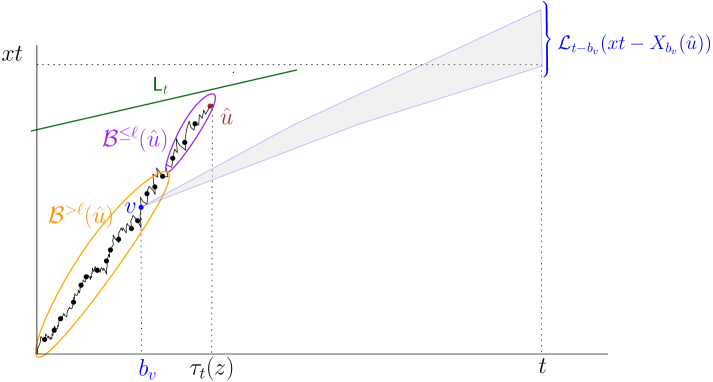
Figure 2. The sets $\mathcal{B}^{>\ell}(\hat{u})$ and $\mathcal{B}^{\leq\ell}(\hat{u})$

For any two particles $u$, $v$ in the BBM. We denote $v\prec u$ if $v$ is an ancestor of $u$; and $v\preceq u$ if either $v\prec u$ or $v=u$. Define

$$\mathcal{B}(u):=\{v:\exists\,u^{\prime}\preceq u\text{ s.t. }v\text{ is the brother of }u^{\prime}\}\cup\{u\}.$$ (4.3)

Let $\hat{u}$ denote the particle alive at time $\tau_{t}(z)$ that has the lowest position, i.e.,

$$\hat{u}=\hat{u}(t,z):=\operatorname*{arg\,min}_{u\in\mathcal{N}_{\tau_{t}(z)}}V_{\tau_{t}(z)}(u).$$ (4.4)

Throughout this section, for each $v\in\mathcal{B}(\hat{u})$, we define

$$b_{v}=b_{v}(\hat{u},\mathcal{B}(\hat{u})):=\begin{cases}\text{the birth time of }v,&\text{ if }v\in\mathcal{B}(\hat{u})\backslash\{\hat{u}\}\\ \tau_{t}(z),&\text{ if }v=\hat{u}.\end{cases}$$ (4.5)

We divide $\mathcal{B}(\hat{u})$ into two subsets according to their genealogical distance to $\hat{u}$ (see Figure 2). For $\ell<\tau_{t}(z)$, define:

$$\mathcal{B}^{>\ell}(\hat{u}) :=\{v\in\mathcal{B}(\hat{u}):b_{v}<\tau_{t}(z)-\ell\}\ ,\text{ and }$$ (4.6)

$$\mathcal{B}^{\leq\ell}(\hat{u}) :=\{v\in\mathcal{B}(\hat{u}):\tau_{t}(z)-\ell\leq b_{v}<\tau_{t}(z)\}.$$ (4.7)

Next, we introduce truncated versions of $\mathscr{L}_{t}[xt,\infty)$ and $W_{\infty}(\theta)$: For $\ell<\tau_{t}(z)$, define:

$$\mathscr{L}_{t}^{>\ell}(xt):=\sum_{v\in\mathcal{B}^{>\ell}(\hat{u})}\mathscr{L}^{(v)}_{t-b_{v}}(xt-X_{b_{v}}(\hat{u}))\ \text{ and }\ W^{>\ell}_{\infty}(\theta):=\sum_{v\in\mathcal{B}^{>\ell}(\hat{u})}e^{-V_{b_{v}}(\hat{u})}W^{(v)}_{\infty}(\theta).$$ (4.8)

In the following, for simplicity, we set $\Gamma[t,z]:=-\psi^{\prime}(\kappa)s+[z,z+1)\ \text{ for }z\in\mathbb{R}$.

Lemma 4.1.

For any fixed $R>0$, the following assertions hold:

1. For any $\epsilon>0$, uniformly in $|z|\leq R$ we have

   $$\lim_{\ell\to\infty}\limsup_{t\to\infty}e^{I(x,a)t}\,\mathbf{P}\left(\mathscr{L}_{t}^{>\ell}(xt)\geq\frac{\epsilon}{\sqrt{t}}e^{at},\mathbf{I}\in\Gamma[t,z]\right)=0,$$ (4.9)

   $$\lim_{\ell\to\infty}\limsup_{t\to\infty}e^{I(x,a)t}\,\mathbf{P}\left(W_{\infty}^{>\ell}(\theta)\geq\epsilon\,e^{\psi^{\prime}(\kappa)s},\mathbf{I}\in\Gamma[t,z]\right)=0.$$ (4.10)

2. For any fixed $K>0$, uniformly in $|z|\leq R$, we have

   $$\lim_{\ell\to\infty}\limsup_{t\to\infty}e^{I(x,a)t}\,\mathbf{P}\left(\min_{v\in\mathcal{B}^{>\ell}(\hat{u})}\{V_{b_{v}}(\hat{u})+\mathbf{I}^{(v)}\}\leq\mathbf{I}+K,\mathbf{I}\in\Gamma[t,z]\right)=0,$$ (4.11)

3. Uniformly in $|z|\leq R$ we have

   $$\lim_{\ell\to\infty}\limsup_{t\to\infty}e^{I(x,a)t}\,\mathbf{P}\bigg{(}\max_{v\in\mathcal{B}^{>\ell}(\hat{u})} \{X_{b_{v}}(\hat{u})+M^{(v)}_{t-b_{v}}\}$$ (4.12)

   $$\geq X_{\tau_{t}(z)}(\hat{u})+\sqrt{2}[t-\tau_{t}(z)],\mathbf{I}\in\Gamma[t,z]\bigg{)}=0.$$ (4.13)

Naturally we define

$$\mathscr{L}_{t}^{\leq\ell}(xt) :=\mathscr{L}_{t}(xt)-\mathscr{L}_{t}^{>\ell}(xt)=\sum_{v\in\mathcal{B}^{\leq\ell}(\hat{u})}\mathscr{L}^{(v)}_{t-b_{v}}(xt-X_{b_{v}}(\hat{u})),$$ (4.14)

$$W_{\infty}^{\leq\ell}(\theta) :=W_{\infty}(\theta)-W^{>\ell}_{\infty}(\theta)=\sum_{v\in\mathcal{B}^{\leq\ell}(\hat{u})}e^{-V(v)}W^{(v)}_{\infty}(\theta).$$ (4.15)

In the following, we use the standard notation $A\operatorname{\triangle}B:=(A\backslash B)\cup(B\backslash A)$.

Lemma 4.2.

Let $c_{\theta}:=\theta\sqrt{2\pi(1-p)}$. Fix $y>0$, $\ell>0$ and $R>0$. For any given small $\epsilon>0$, uniformly in $|z|\leq R$ and $|\lambda_{i}-1|<\epsilon$, $i=1,2$ we have

$$\lim_{\epsilon\downarrow 0}\limsup_{t\to\infty}e^{I(x,a)t}\mathbf{P}\left(\left\{\mathscr{L}_{t}^{\leq\ell}(xt)\geq\frac{\lambda_{1}y\,e^{at}}{\sqrt{t}}\right\}\operatorname{\triangle}\left\{W^{\leq\ell}_{\infty}(\theta)\geq c_{\theta}\lambda_{2}ye^{\psi^{\prime}(\kappa)s}\right\},\mathbf{I}\in\Gamma[t,z]\right)=0.$$ (4.16)

Based on Lemma 4.1 and Lemma 4.2, now we are ready to prove Theorem 1.1.

Proof of Theorem 1.1.

Fix an arbitrary small $\delta>0$ and a value $\lambda\in(0,1)$. According to Proposition 3.1, there exists large constant $R_{\delta}>0$ satisfying that for all $R\geq R_{\delta}$

$$\limsup_{t\to\infty}e^{I(x,a)t}\left|\mathbf{P}\left(\mathscr{L}_{t}(xt)\geq\frac{y}{\sqrt{t}}e^{at}\right)-\sum_{|z|\leq R}\mathbf{P}\left(\mathscr{L}_{t}(xt)\geq\frac{y}{\sqrt{t}}e^{at},\mathbf{I}\in\Gamma[t,z]\right)\right|<\delta.$$ (4.17)

We assert that for each fixed $R>0$ and $|z|\leq R$, as $t\to\infty$

$$\mathrm{Pr}_{\eqref{eq-level-set-min}}(t,z):=e^{I(x,a)t}\mathbf{P}\left(\left\{\mathscr{L}_{t}(xt)\geq\frac{y\,e^{at}}{\sqrt{t}}\right\}\operatorname{\triangle}\left\{W_{\infty}(\theta)\geq c_{\theta}ye^{\psi^{\prime}(\kappa)s}\right\},\mathbf{I}\in\Gamma[t,z]\right)\to 0.$$ (4.18)

As a result of the above and the fact that $|\mathbf{P}(A)-\mathbf{P}(B)|\leq\mathbf{P}(A\operatorname{\triangle}B)$, we can say that uniformly in $|z|\leq R$,

$$\lim_{t\to\infty}e^{I(x,a)t}\mathbf{P}\left(\mathscr{L}_{t}(xt)\geq\frac{y}{\sqrt{t}}e^{at},\mathbf{I}\in\Gamma[t,z]\right)$$ (4.19)

$$=\lim_{t\to\infty}e^{I(x,a)t}\mathbf{P}\left(W_{\infty}(\theta)\geq c_{\theta}ye^{\psi^{\prime}(s)},\mathbf{I}\in-\psi^{\prime}(\kappa)s+(z-1,z]\right)$$ (4.20)

$$=c_{\mathbf{I}}\int_{0}^{1}\mathbf{P}\left(Z\geq c_{\theta}y\,e^{z+1-h}\right)e^{\kappa(z+1-h)}\mathop{}\!\mathrm{d}h=c_{\mathbf{I}}\int_{e^{z}}^{e^{z+1}}\mathbf{P}\left(Z\geq c_{\theta}y\,\gamma\right)\gamma^{\kappa-1}\mathop{}\!\mathrm{d}\gamma.$$ (4.21)

Above, the second equality comes from the following two points: First, by Lemma 2.3,

$$\lim_{t\to\infty}\mathbf{P}\left(W_{\infty}(\theta)\geq c_{\theta}y\,e^{\psi^{\prime}(\kappa)s},\mathbf{I}+\psi^{\prime}(\kappa)s-z-1\in(-1,0]\mid\mathbf{I}\leq-\psi^{\prime}(\kappa)s+z+1\right)$$ (4.22)

$$=\lim_{t\to\infty}\int_{0}^{1}\mathbf{P}\left(e^{\mathbf{I}}W_{\infty}(\theta)\geq c_{\theta}y\,e^{z+1-h},z+1-\mathbf{I}-\psi^{\prime}(\kappa)s\in\mathop{}\!\mathrm{d}h\mid\mathbf{I}\leq-\psi^{\prime}(\kappa)s+z+1\right)$$ (4.23)

$$=\int_{0}^{1}\mathbf{P}\left(Z\geq c_{\theta}y\,e^{z+1-h}\right)e^{-\kappa h}\mathop{}\!\mathrm{d}h.$$ (4.24)

Second, by use of Lemma 2.8 we have

$$\lim_{t\to\infty}e^{I(x,a)t}\mathbf{P}\left(\mathbf{I}\leq-\psi^{\prime}(\kappa)s+z+1\right)=\lim_{t\to\infty}c_{\mathbf{I}}e^{I(x,a)t-\kappa\psi^{\prime}(\kappa)s}e^{\kappa(z+1)}=c_{\mathbf{I}}\,e^{\kappa(z+1)}.$$ (4.25)

Notice that by Lemma 2.3 we have $c_{\mathbf{I}}\mathbf{E}[Z^{\kappa}]=C_{W_{\infty}(\theta)}$, we obtain

$$c_{\mathbf{I}}\sum_{|z|\leq R}\int_{e^{z}}^{e^{z+1}}\mathbf{P}\left(Z\geq c_{\theta}y\gamma\right)\gamma^{\kappa-1}\mathop{}\!\mathrm{d}\gamma\overset{R\to\infty}{\longrightarrow}\frac{c_{\mathbf{I}}}{(c_{\theta}y)^{\kappa}}\mathbf{E}\left[Z^{\kappa}\right]=\frac{C_{W_{\infty}(\theta)}}{(c_{\theta}y)^{\kappa}}.$$ (4.26)

So letting $R\to\infty$ in (4.17), by combining all computations, we arrive at:

$$\frac{C_{W_{\infty}(\theta)}}{(c_{\theta}y)^{\kappa}}-\delta \leq\liminf_{t\to\infty}e^{I(x,a)t}\mathbf{P}\left(\mathscr{L}_{t}(xt)\geq\frac{y}{\sqrt{t}}e^{at}\right)$$ (4.27)

$$\leq\limsup_{t\to\infty}e^{I(x,a)t}\mathbf{P}\left(\mathscr{L}_{t}(xt)\geq\frac{y}{\sqrt{t}}e^{at}\right)\leq\frac{C_{W_{\infty}(\theta)}}{(c_{\theta}y)^{\kappa}}+\delta.$$ (4.28)

By sending $\delta\downarrow 0$, we get Theorem 1.1. Now it remains to prove the claim (4.18).

Let us fix an arbitrary small $\epsilon\in(0,1)$ and an arbitrary small $\delta>0$. Let

$$E_{\ell,\epsilon}:=\left\{\mathscr{L}^{>\ell}_{t}(xt)\leq\frac{\epsilon\,y}{\sqrt{t}}e^{at},W^{>\ell}_{\infty}(\theta)\leq\epsilon c_{\theta}y\,e^{\psi^{\prime}(\kappa)s}\right\}.$$ (4.29)

By use of Lemma 4.1, there is a constant $\ell(\lambda,\delta,R)$ such that for every $\ell\geq\ell(\lambda,\delta,R)$, and for sufficiently large $t$, the following holds

$$e^{I(x,a)t}\,\mathbf{P}\left(E_{\ell,\epsilon}^{c},\mathbf{I}\in\Gamma[t,z]\right)<\delta,\forall\,|z|\leq R.$$ (4.30)

When $E_{\ell,\epsilon}$ occurs, if $\mathscr{L}_{t}(xt)\geq\frac{y\,e^{at}}{\sqrt{t}}$ but $W_{\infty}(\theta)\leq c_{\theta}ye^{\psi^{\prime}(\kappa)s}$, we must have $\mathscr{L}^{>\ell}_{t}(xt)\geq\frac{(1-\epsilon)y}{\sqrt{t}}e^{at}$ and $W_{\infty}^{>\ell}(\theta)\leq c_{\theta}ye^{\psi^{\prime}(\kappa)s}$. Similarly if $\mathscr{L}_{t}(xt)\leq\frac{y\,e^{at}}{\sqrt{t}}$ but $W_{\infty}(\theta)\geq c_{\theta}ye^{\psi^{\prime}(\kappa)s}$, we have $\mathscr{L}^{\leq\ell}_{t}(xt)\leq\frac{y}{\sqrt{t}}e^{at}$ and $W_{\infty}^{\leq\ell}(\theta)\geq c_{\theta}(1-\epsilon)ye^{\psi^{\prime}(\kappa)s}$. In summary, we conclude

$$\mathrm{Pr}_{\eqref{eq-level-set-min}}(t,z) \leq e^{I(x,a)t}\mathbf{P}\left(E_{\ell,\epsilon}^{c},\mathbf{I}\in\Gamma[t,z]\right)$$ (4.31)

$$+e^{I(x,a)t}\mathbf{P}\left(\left\{\mathscr{L}^{\leq\ell}_{t}(xt)\geq\frac{(1-\epsilon)y}{\sqrt{t}}e^{at}\right\}\operatorname{\triangle}\left\{W_{\infty}^{\leq\ell}(\theta)\geq c_{\theta}ye^{\psi^{\prime}(\kappa)s}\right\},\mathbf{I}\in\Gamma[t,z]\right)$$ (4.32)

$$+e^{I(x,a)t}\mathbf{P}\left(\left\{\mathscr{L}^{\leq\ell}_{t}(xt)\leq\frac{y}{\sqrt{t}}e^{at}\right\}\operatorname{\triangle}\left\{W_{\infty}^{\leq\ell}(\theta)\geq c_{\theta}(1-\epsilon)ye^{\psi^{\prime}(\kappa)s}\right\},\mathbf{I}\in\Gamma[t,z]\right).$$ (4.33)

Now by use of Lemma 4.2, taking the limit as $t\to\infty$ followed by $\epsilon\downarrow 0$, we obtain that $\limsup_{t\to\infty}\mathrm{Pr}_{\eqref{eq-level-set-min}}(t,z)\leq\delta$ uniformly in $z\in[-R,R]$. Since $\delta$ is arbitrary, the desired result (4.18) follows. This completes the proof. ∎

4.2. Change of measure

In this section, we apply the change of measure technique outlined in §2.1 with the additive martingale with parameter $b$

$$W_{r}(b)=\sum_{u\in\mathcal{N}_{r}}e^{bX(u)-\left(\frac{b^{2}}{2}+1\right)r}=\sum_{u\in\mathcal{N}_{r}}e^{-\kappa V(u)},\,r>0.$$ (4.34)

We begin by introducing a stopping time for the BBM with a spine ($\{X_{r}(u):u\in\mathcal{N}_{r}\},w_{r})_{r\geq 0}$ defined by

$$\tau^{w}(z):=\inf\{r>0:V_{r}(w)=-\psi^{\prime}(\kappa)s+z\}.$$ (4.35)

Denote by $\hat{w}$ the spine particle at the stopping time $\tau^{w}(z)$ when it is finite, i.e., $\hat{w}:=w_{\tau^{w}(z)}$.

Lemma 4.3.

For any $t>1$, $r\geq 1$, $z\in\mathbb{R}$, and $A\in\mathcal{F}_{\infty}$,

$$e^{I(x,a)t}\mathbf{P}\left(A,\tau(z)<r\right)=e^{\kappa z}(\mathbf{Q}^{b,*}_{\tau^{w}(z)}\otimes\mathbf{P})\left(A,\tau^{w}(z)=\tau(z)<r\right).$$ (4.36)

In the following except for the proof of this lemma, we will omit the parameter $b$ and write $\mathbf{Q}^{b,*}_{\tau^{w}(z)}\otimes\mathbf{P}$ as $\mathbf{Q}^{*}_{\tau^{w}(z)}\otimes\mathbf{P}$, since only this parameter is used.

Proof.

Consider the measure $\mathbf{Q}^{b,*}_{\tau_{r}(z)}\otimes\mathbf{P}$ defined via the stopping time $\tau_{r}(z)=\tau(z)\wedge r$. From the definition of the density (2.4), we have

$$(\mathbf{Q}^{b,*}_{\tau_{r}(z)}\otimes\mathbf{P})(\cdot\cap\{\tau_{n}(z)=\tau^{w}(z)\})=(\mathbf{Q}^{b,*}_{\tau^{w}(z)}\otimes\mathbf{P})(\cdot\cap\{\tau_{r}(z)=\tau^{w}(z)\}).$$ (4.37)

Note that, almost surely, if $\tau(z)<\infty$, exactly one particle of the BBM will reach the line $-\psi^{\prime}(\kappa)s+z$ at time $\tau(z)$. In other words, we have

$$\mathbf{1}_{\left\{\tau(z)<r\right\}}=\sum_{u\in\mathcal{N}_{\tau(z)}}\mathbf{1}_{\left\{\tau^{u}(z)=\tau(z)<r\right\}}\ \text{ a.s.}$$ (4.38)

where $\tau^{u}(z):=\inf\{0<t<d_{u}:V_{t}(u)=-\psi^{\prime}(s)+z\}$ (recall that $d_{u}$ denotes the death time of $u$). By using (2.5) from Lemma 2.1, we deduce that

$$\mathbf{P}\left(A,\tau(z)<r\right)=\mathbf{E}_{\mathbf{Q}^{b,*}_{\tau_{r}(z)}\otimes\mathbf{P}}\left[\sum_{u\in\tau_{r}(z)}\frac{e^{-\kappa V_{\tau_{r}(z)}(u)}}{W_{\tau_{r}(z)}(b)}e^{\kappa V_{\tau_{r}(z)}(u)}\mathbf{1}_{\left\{\tau^{u}(z)=\tau(z)<r\right\}}\mathbf{1}_{\left\{A\right\}}\right].$$ (4.39)

Applying (2.6) of Lemma 2.1 to the inequality above, we obtain that

$$\mathbf{P}\left(A,\tau(z)<r\right) =\mathbf{E}_{\mathbf{Q}^{b,*}_{\tau_{r}(z)}\otimes\mathbf{P}}\left[e^{\kappa V_{\tau^{w}(z)}(w)}\mathbf{1}_{\left\{\tau^{w}(z)=\tau(z)<r\right\}}\mathbf{1}_{\left\{A\right\}}\right]$$ (4.40)

$$=e^{-I(x,a)t+\kappa z}(\mathbf{Q}^{b,*}_{\tau_{r}(z)}\otimes\mathbf{P})\left(\tau^{w}(z)=\tau(z)<r,A\right).$$ (4.41)

Above, we have used the fact that $V_{\tau^{w}(z)}(w)=-\psi^{\prime}(\kappa)s+z$ and $\kappa\psi^{\prime}(\kappa)s=I(x,a)t$. This completes the proof. ∎

Note that on the event $\tau^{w}(z)=\tau(z)<t$ we have $\hat{u}=\hat{w}$. This observation leads us to an immediate and useful corollary of Lemma 4.3.

Corollary 4.4.

For $L\geq 1$, define

$$G_{L}^{1}:=\{|\tau(z)-s|\leq L\sqrt{s}\},\ L\geq 1.$$ (4.42)

Then for any $t>0$, $z\in\mathbb{R}$, and $A\in\mathcal{F}_{\infty}$, we have

$$e^{I(x,a)t}\mathbf{P}\left(A,G^{1}_{L},\mathbf{I}\in\Gamma[t,z]\right)=e^{\kappa z}(\mathbf{Q}^{*}_{\tau^{w}(z)}\otimes\mathbf{P})\left(A,G^{1}_{L}(w),I_{0}^{w}\right).$$ (4.43)

where $G^{1}_{L}(w):=\{|\tau^{w}(z)-s|\leq L\sqrt{s}\}$ and

$$I_{0}^{w} :=\{\mathbf{I}+\psi^{\prime}(\kappa)s\in[z,z+1]\}\cap\{\tau^{w}(z)=\tau(z)\}$$ (4.44)

$$=\{\tau^{w}(z)=\tau(z)\}\cap\bigcap_{v\in\mathcal{B}(\hat{w})}\{\mathbf{I}^{(v)}>V_{\tau^{w}(z)}(w)-1-V_{b_{v}}(w)\}.$$ (4.45)

Lemma 4.5.

For $\ell>0$, $L\geq 1$, define

$$G_{\ell,L}^{2}:=\left\{|\mathcal{B}^{\leq\ell}(\hat{u})|\leq L\right\}\cap\left\{\forall\,r\in[\tau(z)-\ell,\tau(z)],|V_{r}(\hat{u})-V_{\tau(z)}(\hat{u})|\leq L\right\}.$$ (4.46)

Let $G_{\ell,L}:=G_{L}^{1}\cap G_{\ell,L}^{2}$. Then for fixed $\ell>0$, $R>0$ we have

$$\lim_{L\to\infty}\limsup_{t\to\infty}\sup_{|z|\leq R}e^{I(x,a)t}\,\mathbf{P}\left(\mathbf{I}\in\Gamma[t,z],G_{\ell,L}^{c}\right)=0.$$ (4.47)

To prove this lemma, we need to use a well-known fact about the first passage times of Brownian motion:

Lemma 4.6.

Let $(\beta_{t}=\nu t-\sigma B_{t}:t\geq 0)$ where $B_{t}$ is a standard Brownian motion and $\nu,\sigma>0$. Them the first passage time $T(\alpha):=\inf\left\{t>0:\beta_{t}=\alpha\right\}$ for a fixed level $\alpha>0$ by $X_{t}$ is distributed according to an inverse Gaussian $(\frac{\alpha}{\nu},\frac{\alpha^{2}}{\sigma^{2}})$. That is, $T(\alpha)$ has p.d.f.

$$f_{\frac{\alpha}{\nu},\frac{\alpha^{2}}{\sigma^{2}}}(T):=\frac{\alpha}{\sigma\sqrt{2\pi T^{3}}}\exp\left(-\frac{(\alpha-\nu T)^{2}}{2\sigma^{2}T}\right),\ T>0.$$ (4.48)

Proof of Lemma 4.5.

We begin by asserting that

$$\mathrm{Pr}_{\eqref{eq-G-estimate}}(L):=\limsup_{t\to\infty}\sup_{|z|\leq R}e^{I(x,a)t}\,\mathbf{P}\left(\mathbf{I}\in\Gamma[t,z],G^{1}_{L}\right)\lesssim_{R,x,a}e^{-\frac{\psi^{\prime}(\kappa)^{2}}{2\psi^{\prime\prime}(\kappa)}L^{2}}.$$ (4.49)

In fact, since the event $\mathbf{I}\in\Gamma[t,z]$ implies that $\tau(z)<\infty$, it follows from Lemma 4.3 that

$$e^{I(x,a)t}\,\mathbf{P}\left(\mathbf{I}\in\Gamma[t,z],|\tau(z)-s|>L\sqrt{s}\right)\lesssim_{R}(\mathbf{Q}^{*}_{\tau^{w}(z)}\otimes\mathbf{P})\left(|\tau^{w}(z)-s|>L\sqrt{s}\right).$$ (4.50)

Under $\mathbf{Q}^{*}_{\tau^{w}(z)}\otimes\mathbf{P}$, $(V_{r}(w):r\leq\tau^{w}(z))$ is a Brownian motion with drift $-\psi^{\prime}(\kappa)$ and diffusion coefficient $\psi^{\prime\prime}(\kappa)$ stopped upon hitting the line $-\psi^{\prime}(\kappa)s+z$. By applying Lemma 4.6 we obtain

$$e^{I(x,a)t}\,\mathbf{P}\left(\mathbf{I}\in\Gamma[t,z],|\tau(z)-s|>L\sqrt{s}\right)$$ (4.51)

$$\lesssim_{R}\int_{\mathbb{R}_{+}\backslash[s-L\sqrt{s},s+L\sqrt{s}]}\frac{\psi^{\prime}(\kappa)s-z}{\sqrt{2\pi\psi^{\prime\prime}(\kappa)T^{3}}}\exp\left(-\frac{(\psi^{\prime}(\kappa)s-z-\psi^{\prime}(\kappa)T)^{2}}{2\psi^{\prime\prime}(\kappa)T}\right)\mathop{}\!\mathrm{d}T$$ (4.52)

$$\lesssim_{x,a}\int_{(-\sqrt{s},\infty])\backslash[-L,L]}\sqrt{s}\,\frac{\psi^{\prime}(\kappa)s-z}{\sqrt{(s+\lambda\sqrt{s})^{3}}}\exp\left(-\frac{1}{2\psi^{\prime\prime}(\kappa)}\frac{[\psi^{\prime}(\kappa)\lambda+z/\sqrt{s}]^{2}}{1+\lambda/\sqrt{s}}\right)\mathop{}\!\mathrm{d}\lambda.$$ (4.53)

Above, we have made a change of variable $T=s+\lambda\sqrt{s}$. By employing the dominated convergence theorem, we conclude that

$$\mathrm{Pr}_{\eqref{eq-G-estimate}}(L)\lesssim_{R,x,a}\int_{L}^{\infty}e^{-\frac{\psi^{\prime}(\kappa)^{2}}{2\psi^{\prime\prime}(\kappa)}\lambda^{2}}\mathop{}\!\mathrm{d}\lambda\lesssim_{x,a}e^{-\frac{\psi^{\prime}(\kappa)^{2}}{2\psi^{\prime\prime}(\kappa)}L^{2}}.$$ (4.54)

Next, by applying (4.43) and observing that $\hat{u}=\hat{w}$ on $G^{1}_{L}(w)\cap I_{0}^{w}$, we have

$$e^{I(x,a)t}\,\mathbf{P}\left(\mathbf{I}\in\Gamma[t,z],G^{1}_{L}\backslash G^{2}_{\ell,L}\right)\leq e^{\kappa R}(\mathbf{Q}^{*}_{\tau^{w}(z)}\otimes\mathbf{P})\left(G^{1}_{L}(w)\backslash G^{2}_{\ell,L}(w)\right),$$ (4.55)

where $G_{\ell,L}^{2}(w):=\left\{|\mathcal{B}^{\leq\ell}(\hat{w})|\leq L\right\}\cap\left\{\forall\,r\in[\tau^{w}(z)-\ell,\tau^{w}(z)],|V_{r}(w)-V_{\tau^{w}(z)}(w)|\leq L\right\}$. First, observe that for a fixed $\ell$, the law of the random variable $\max\{|V_{r}(w)-V_{\tau^{w}(z)}(w)|:r\in[\tau^{w}(z)-\ell,\tau^{w}(z)]\}$ does not depend on $t,z$ and it is tight. Second, conditioned on $\tau^{w}(z)$ and $\{V_{r}(w):r\leq\tau^{w}(z)\}$, times of branching events along the spine $(b_{v}=b_{v}:v\in\mathcal{B}(\hat{w})\backslash\{\hat{w}\})$ form a Poisson process with rate Poisson process with rate $2$ on $[0,\tau^{w}(z)]$. Thus the number of branching points in the time interval $[\tau^{w}(z)-\ell,\tau^{w}(z)]$ does not depend on $t$ or $z$ and is also tight. Hence, for every $\ell\geq 1$, uniformly in $z$, we have

$$\lim_{L\to\infty}\limsup_{t\to\infty}\sup_{|z|\leq R}(\mathbf{Q}^{*}_{\tau^{w}(z)}\otimes\mathbf{P})\left(G^{1}_{L}(w)\backslash G^{2}_{\ell,L}(w)\right)=0.$$ (4.56)

This, together with (4.49) and (4.55), implies the desired result. ∎

4.3. Proofs of Lemmas in Section 4.1

Proof of Lemma 4.1.

We will first prove (4.9) and (4.13). A similar argument can be applied to prove (4.10) and (4.11) (alternatively, see [CdRM24, Lemmas 3.7 and 3.3] for a proof in the context of branching random walks).

Proof of (4.9). Thanks to Lemma 4.5, it is sufficient to show that for each fixed $L\geq 1$, uniformly in $|z|\leq R$, we have

$$\lim_{\ell\to\infty}\limsup_{t\to\infty}e^{I(x,a)t}\,\mathbf{P}\left(\mathscr{L}_{t}^{>\ell}(xt)\geq\frac{\epsilon}{\sqrt{t}}e^{at},\mathbf{I}\in\Gamma[t,z],G_{L}^{1}\right)=0.$$ (4.57)

Applying (4.43) with $A=\{\mathscr{L}_{t}^{>\ell}(xt)\geq\frac{\epsilon}{\sqrt{t}}e^{at}\}$, the expression above becomes

$$\lim_{\ell\to\infty}\limsup_{t\to\infty}(\mathbf{Q}^{*}_{\tau^{w}(z)}\otimes\mathbf{P})\left(\mathscr{L}_{t}^{>\ell}(xt)\geq\frac{\epsilon}{\sqrt{t}}e^{at},I_{0}^{w},G^{1}_{L}(w)\right)=0.$$ (4.58)

On the event $I_{0}^{w}\cap G^{1}_{L}(w)$, since $\hat{u}=\hat{w}$, we can rewrite $\mathscr{L}_{t}^{>\ell}(xt)$ as $\sum_{v\in\mathcal{B}^{>\ell}(\hat{w})}\mathscr{L}^{(v)}_{t-b_{v}}(xt-X_{b_{v}}(w))$. So it suffices to show that for any fixed $L\geq 1$, uniformly in $|z|\leq R$,

$$\lim_{\ell\to\infty}\limsup_{t\to\infty}(\mathbf{Q}^{*}_{\tau^{w}(z)}\otimes\mathbf{P})\left(\sum_{v\in\mathcal{B}^{>\ell}(\hat{w})}\mathscr{L}^{(v)}_{t-b_{v}}(xt-X_{b_{v}}(w))\geq\frac{\epsilon}{\sqrt{t}}e^{at},I_{0}^{w},G^{1}_{L}(w)\right)=0.$$ (4.59)

We claim that on $I_{0}^{w}\cap G^{1}_{L}(w)$, $xt-X_{r}(w)=\Theta(t)$ for all $r\leq\tau^{w}(z)$. In fact, by definition for every $r\leq\tau^{w}(z)$, we have $V_{r}(w)>-\psi^{\prime}(\kappa)s+z$, which implies $\theta X_{r}(w)\leq(\frac{\theta^{2}}{2}+1)r+\psi^{\prime}(\kappa)s-z\leq 2s+O(\sqrt{s})+R$. Thus, we get $X_{r}(w)\leq bs+O(\sqrt{s})+O(1)$. Next, let $\mathcal{G}^{*}_{\tau^{w}(z)}:=\sigma(V_{r}(w):r\leq\tau^{w}(z),b_{v},v\in\mathcal{B}(\hat{w}))$ denote the $\sigma$-field that contains the information about the movement and branching times of the spine particles up to time $\tau^{w}(z)$. Conditionally on $\mathcal{G}^{*}_{\tau^{w}(z)}$, by using the branching property, the many-to-one formula, and the Gaussian tail inequality $\mathbf{P}(N(0,1)>y)\leq\frac{1}{y\sqrt{2\pi}}e^{-y^{2}/2},\forall\,y>0$, we obtain, on the event $G^{1}_{L}(w)\in\mathcal{G}^{*}_{\tau^{w}(z)}$,

$$\mathbf{E}_{\mathbf{Q}^{*}_{\tau^{w}(z)}\otimes\mathbf{P}}\left(\sum_{v\in\mathcal{B}^{>\ell}(\hat{w})}\mathscr{L}^{(v)}_{t-b_{v}}(xt-X_{b_{v}}(w))\mid\mathcal{G}^{*}_{\tau^{w}(z)}\right)$$ (4.60)

$$\lesssim\sum_{b_{v}\leq\tau^{w}(z)-\ell}\,\frac{\sqrt{t-b_{v}}}{xt-X_{b_{v}}(w)}\exp\left\{(t-b_{v})-\frac{[xt-\mathsf{L}_{t}(b_{v})+\mathsf{L}_{t}(b_{v})-X_{b_{v}}(w)]^{2}}{2(t-b_{v})}\right\}$$ (4.61)

$$\lesssim_{x,a}\frac{1}{\sqrt{t}}e^{at}\sum_{b_{v}\leq\tau^{w}(z)-\ell}\,\exp\left\{-\frac{xt-\mathsf{L}_{t}(b_{v})}{t-b_{v}}[\mathsf{L}_{t}(b_{v})-X_{b_{v}}(w)]\right\}$$ (4.62)

Above in the last inequality, we have used the fact that (see (1.14) for the definition of $\mathsf{F}_{t}$)

$$t-b_{v}-\frac{[xt-\mathsf{L}_{t}(b_{v})]^{2}}{2(t-b_{v})}\leq(t-b_{v})-\frac{[xt-\mathsf{F}_{t}(b_{v})]^{2}}{2(t-b_{v})}=at,$$ (4.63)

as $\mathsf{L}_{t}(r)\leq\mathsf{F}_{t}(r)\ll xt$ for all $r\leq\tau^{w}(z)\leq s+L\sqrt{s}$.

We denote the probability in (4.59) by $Q_{\eqref{eq-distant-relative-2}}(t,\ell)$. By (4.62) and applying Markov’s inequality, we obtain,

$$Q_{\eqref{eq-distant-relative-2}}(t,\ell)\lesssim_{x,a}\frac{1}{\epsilon}\,\mathbf{E}_{\mathbf{Q}^{*}_{\tau^{w}(z)}\otimes\mathbf{P}}\left[\min\left\{1,\sum_{b_{v}\leq\tau^{w}(z)-\ell}\,e^{-\frac{xt-\mathsf{L}_{t}(b_{v})}{t-b_{v}}[\mathsf{L}_{t}(b_{v})-X_{b_{v}}(w)]}\right\}\mathbf{1}_{\left\{G^{1}_{L}(w)\right\}}\right].$$ (4.64)

We choose an arbitrary constant $c_{0}=c_{0}(x,a)>0$ satisfying $0<c_{0}<\psi^{\prime}(\kappa)$. Define

$$G^{4}_{\ell}(w):=\{\forall r\in(\ell,\tau^{w}(z)],V_{\tau^{w}(z)-r}(w)-V_{\tau^{w}(z)}(w)\geq c_{0}r\}.$$ (4.65)

See also Figure 3. We claim that there is deterministic sequence $\{\delta(\ell):\ell\geq 1\}$ with $\delta(\ell)\to 0$ as $\ell\to\infty$ such that

$$(\mathbf{Q}^{*}_{\tau^{w}(z)}\otimes\mathbf{P})\left(G_{L}^{1}(w)\backslash G_{\ell}^{4}(w)\right)\geq 1-\delta(\ell).$$ (4.66)

Then on $G_{L}^{4}(w)$ for any $r\in[0,\tau^{w}(z)-\ell)$ we have $V_{r}(w)+\psi^{\prime}(\kappa)s\geq c_{0}[\tau^{w}(z)-r]+z$. Noting that $\theta[\mathsf{L}_{t}(r)-X_{r}(w)]=V_{r}(w)+\psi^{\prime}(\kappa)s$, this yields $\mathsf{L}_{t}(r)-X_{r}(w)\geq[c_{0}(\tau^{w}(z)-r)+z]/\theta$. Besides, for large $t$, we have $\frac{xt-\mathsf{L}_{t}(r)}{t-r}\geq\frac{\theta}{2}$ for every $r\leq s+L\sqrt{s}$. Thus we conclude

$$Q_{\eqref{eq-distant-relative-2}}(t,\ell)\lesssim_{x,a}(\mathbf{Q}^{*}_{\tau^{w}(z)}\otimes\mathbf{P})(G_{L}^{1}(w)\backslash G_{\ell}^{4}(w))$$ (4.67)

$$\qquad\qquad\qquad+\mathbf{E}_{\mathbf{Q}^{*}_{\tau^{w}(z)}\otimes\mathbf{P}}\left[\sum_{b_{v}\leq\tau^{w}(z)-\ell}\,e^{-\frac{xt-\mathsf{L}_{t}(b_{v})}{\theta(t-b_{v})}[c_{0}(\tau^{w}(z)-b_{v})+z]}\mathbf{1}_{\left\{G_{L}^{1}(w)\cap G^{4}_{\ell}(w)\right\}}\right]$$ (4.68)

$$\leq\delta(\ell)+e^{z/2}\mathbf{E}_{\mathbf{Q}^{*}_{\tau^{w}(z)}\otimes\mathbf{P}}\left[\sum_{b_{v}\leq\tau^{w}(z)-\ell}\,e^{-c_{0}\,(\tau^{w}(z)-b_{v})/2}\right]\leq\delta(\ell)+e^{R/2}\int_{\ell}^{\infty}e^{-c_{0}y/2}\mathop{}\!\mathrm{d}y.$$ (4.69)

Above, we have used that conditioned on $\tau^{w}(z)$, $(b_{v}:v\in\mathcal{B}(\hat{w})\backslash\{\hat{w}\})$ forms a Poisson process with rate $2$ on the interval $[0,\tau^{w}(z)]$. Now we can deduce the desired result (4.9).

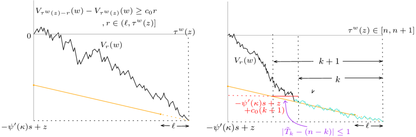
Figure 3. Left: Event $G^{4}_{\ell}(w)$. Right: Event $G^{1}_{L}(w)\backslash G^{4}_{\ell}(w)$.

It remains to show the claim (4.66). In fact, if $G_{L}^{1}(w)\backslash G_{\ell}^{4}(w)$ happen, then there must exist some $k\geq\ell$ such that the process $\{V_{r}(w)\}_{r\geq 0}$ hits the step function $r\mapsto V_{\tau^{w}(z)}(w)+c_{0}\lceil\tau^{w}(z)-r\rceil$ during the time interval $[\tau^{w}(z)-k-1,\tau^{w}(z)-k]$. See Figure 3. Thus the first passaging time at level $V_{\tau^{w}(z)}(w)+c_{0}(k+1)$ by the process $\{V_{r}(w)\}$, say $T^{*}_{k}=T^{V}(-\psi^{\prime}(\kappa)s+z+c_{0}(k+1))$, belongs to $[\tau^{w}(z)-k-1,\tau^{w}(z)-k]$. So if addition $\tau^{w}(z)\in[n,n+1]$, we have $|T^{*}_{k}-(n-k)|\leq 1$ and $V_{n}-V_{T^{*}_{k}}\geq-c_{0}(k+1)$. In conclusion, we can bound $(\mathbf{Q}^{*}_{\tau^{w}(z)}\otimes\mathbf{P})(G_{L}^{1}(w)\backslash G_{\ell}^{4}(w))$ above by

$$\sum_{\begin{subarray}{c}|n-s|\leq L\sqrt{s}\\ \ell\leq k<n\end{subarray}}(\mathbf{Q}^{*}_{\tau^{w}(z)}\otimes\mathbf{P})\left(|T^{*}_{k}-(n-k)|\leq 1,V_{n}(w)-V_{T^{*}_{k}}(w)\geq-c_{0}(k+1),\tau^{w}(z)\in[n,n+1]\right).$$ (4.70)

Let $(W,\mathbf{P})$ denote a Brownian motion with drift $\psi^{\prime}(\kappa)$ diffusion coefficient $\psi^{\prime\prime}(\kappa)$, and let $T^{W}_{k}$ be the first passaging time at level $-\psi^{\prime}(\kappa)s+c_{0}(k+1)$. Since under $\mathbf{Q}^{*}_{\tau^{w}(z)}\otimes\mathbf{P}$, $(V_{r}(w):r\leq\tau^{w}(z))$ has the same law as $W$ stopped upon hitting the line $-\psi^{\prime}(\kappa)s+z$, by using the strong Markov property, we get

$$(\mathbf{Q}^{*}_{\tau^{w}(z)}\otimes\mathbf{P})(G_{L}^{1}(w)\backslash G_{\ell}^{4}(w))$$ (4.71)

$$\leq\sum_{\ell\leq k}\sum_{\begin{subarray}{c}k+1\leq n\\ |n-s|\leq L\sqrt{s}\end{subarray}}\mathbf{P}\left(|T^{W}_{k}-(n-k)|\leq 1\right)\max_{|r|\leq 1}\mathbf{P}\left(W_{k+r}\geq-c_{0}(k+1)\right).$$ (4.72)

By applying the Gaussian tail inequality, we deduce that there exists a constant $c_{1}=c_{1}(x,a)>0$ such that $\max_{|r|\leq 1}\mathbf{P}\left(W_{k+r}\geq-c_{0}(k+1)\right)\lesssim e^{-c_{2}k}$. On the other hand, notice that

$$\sum_{k+1\leq n}\mathbf{P}\left(|T^{W}_{k}-(n-k)|\leq 1\right)\leq 2\sum_{j\geq 1}\mathbf{P}\left(T^{W}_{k}\in[j-1,j]\right)\leq 2.$$ (4.73)

Finally we obtain

$$(\mathbf{Q}^{*}_{\tau^{w}(z)}\otimes\mathbf{P})(G_{L}^{1}(w)\backslash G_{\ell}^{4}(w))\lesssim_{x,a}\sum_{\ell\leq k}e^{-c_{1}k}.$$ (4.74)

as desired. We now completes the proof of (4.9).

Proof of (4.13). Let us define $Q_{\eqref{eq-relative-max-3}}(t,\ell)$ as the following probability:

$$(\mathbf{Q}^{*}_{\tau^{w}(z)}\otimes\mathbf{P})\left(\max_{v\in\mathcal{B}^{>\ell}(\hat{w})}\{X_{b_{v}}(w)+M^{(v)}_{t-b_{v}}\}\geq X_{\tau^{w}(z)}(w)+\sqrt{2}[t-\tau^{w}(z)],I_{0}^{w},G^{1}_{L}(w)\right).$$ (4.75)

As in the proof of (4.9), it is sufficient to show that for any fixed $R>0$, $L\geq 1$, $\lim\limits_{\ell\to\infty}\limsup\limits_{t\to\infty}Q_{\eqref{eq-relative-max-3}}(t,\ell)=0$ uniformly in $|z|\leq R$. We recall a well-known inequality bout the maximal position of the BBM (see [Bra83] or [Aïd13]): $\mathbf{P}(M_{t}\geq\sqrt{2}t+y)\lesssim e^{-\sqrt{2}y}$ for $y\geq 1$. By applying the branching property, conditioned on $\mathcal{G}^{*}_{\tau^{w}(z)}$, for each $v\in\mathcal{B}^{>\ell}(w)$, we have

$$(\mathbf{Q}^{*}_{\tau^{w}(z)}\otimes\mathbf{P})\left(X_{b_{v}}(w)+M^{(v)}_{t-b_{v}}\geq X_{\tau^{w}(z)}(w)+\sqrt{2}[t-\tau^{w}(z)]\mid\mathcal{G}^{*}_{\tau^{w}(z)}\right)\mathbf{1}_{\left\{G^{1}_{L}(w)\right\}}$$ (4.76)

$$\qquad\lesssim_{R}\exp\left\{-\sqrt{2}[\mathsf{L}_{t}(b_{v})-X_{b_{v}}(w)]\right\}\mathbf{1}_{\left\{G^{1}_{L}(w)\right\}},$$ (4.77)

where we have used the facts that $X_{\tau^{w}(z)}(w)=\mathsf{L}_{t}(\tau^{w}(z))-z/\theta$, and hence

$$X_{\tau^{w}(z)}(w)+\sqrt{2}[t-\tau^{w}(z)]-\mathsf{L}_{t}(b_{v})+\mathsf{L}_{t}(b_{v})-X_{b_{v}}(w)$$ (4.78)

$$=\sqrt{2}(t-b_{v})+\frac{(\theta-\sqrt{2})^{2}}{2\theta}\left(\tau^{w}(z)-b_{v}\right)+\mathsf{L}_{t}(b_{v})-X_{b_{v}}(w)-\frac{z}{\theta}.$$ (4.79)

Using the Markov inequality again we finally get

$$Q_{\eqref{eq-relative-max-3}}(t,\ell) \lesssim_{x,a,R}(\mathbf{Q}^{*}_{\tau^{w}(z)}\otimes\mathbf{P})(G_{L}^{1}(w)\backslash G_{\ell}^{4}(w))$$ (4.80)

$$\qquad+\mathbf{E}_{\mathbf{Q}^{*}_{\tau^{w}(z)}\otimes\mathbf{P}}\bigg{[}\sum_{b_{v}\leq\tau^{w}(z)-\ell}\,e^{-\sqrt{2}[c_{0}(\tau^{w}(z)-b_{v})]}\mathbf{1}_{\left\{G_{L}^{1}(w)\cap G^{4}_{\ell}(w)\right\}}\bigg{]}$$ (4.81)

$$\leq\delta(\ell)+e^{R/2}\int_{\ell}^{\infty}e^{-c_{0}y/2}\mathop{}\!\mathrm{d}y.$$ (4.82)

Again we have used that conditioned on $\tau^{w}(z)$, $(b_{v}:v\in\mathcal{B}(\hat{w})\backslash\{\hat{w}\})$ forms a Poisson process with rate $2$ on the interval $[0,\tau^{w}(z)]$. This completes the proof of (4.13). ∎

Proof of Lemma 4.2.

Thanks to Lemma 4.5, it suffices to show that for each fixed $L\geq 1$, uniformly in $|z|\leq R$ and $|\lambda_{i}-1|\leq\epsilon$, $i=1,2$,

$$\lim_{\epsilon\downarrow 0}\limsup_{t\to\infty}e^{I(x,a)t}\mathbf{P}\left(\left\{\mathscr{L}_{t}^{\leq\ell}(xt)\geq\frac{\lambda_{1}e^{at}}{c_{\theta}\sqrt{t}}\right\}\operatorname{\triangle}\left\{W^{\leq\ell}_{\infty}(\theta)\geq\lambda_{2}ye^{\psi^{\prime}(\kappa)s}\right\},\mathbf{I}\in\Gamma[t,z],G_{\ell,L}\right)=0.$$ (4.83)

By applying (4.43) with $A=\{\mathscr{L}_{t}^{\leq\ell}(xt)\geq\frac{\lambda_{1}y}{c_{\theta}\sqrt{t}}e^{at}\}\operatorname{\triangle}\{W^{\leq\ell}_{\infty}(\theta)\geq\lambda_{2}ye^{\psi^{\prime}(\kappa)s}\}\cap G_{\ell,L}^{2}$, to demonstrate (4.83) it is sufficient to show that uniformly in $|z|\leq R$ and $|\lambda_{i}-1|\leq\epsilon$, $i=1,2$,

$$\lim_{\epsilon\downarrow 0}\limsup_{t\to\infty}(\mathbf{Q}^{*}_{\tau^{w}(z)}\otimes\mathbf{P})\left(\left\{\mathscr{L}_{t}^{\leq\ell}(xt)\geq\frac{\lambda_{1}e^{at}}{c_{\theta}\sqrt{t}}\right\}\operatorname{\triangle}\left\{W^{\leq\ell}_{\infty}(\theta)\geq\lambda_{2}ye^{\psi^{\prime}(\kappa)s}\right\},G^{w}_{\ell,L},I_{0}^{w}\right)=0$$ (4.84)

Above we have used the fact that on the event $\{\tau(z)=\tau^{w}(z)<t\}$, we have $\hat{u}=\hat{w}$ and hence $I_{0}^{w}\cap G_{\ell,L}=I_{0}^{w}\cap G_{\ell,L}^{w}$ where

$$G^{w}_{\ell,L}:=G^{1}_{L}(w)\cap\left\{|\mathcal{B}^{\leq\ell}(\hat{w})|\leq L\right\}\cap\left\{\forall\,r\in[\tau^{w}(z)-\ell,\tau^{w}(z)],|V_{r}(w)-V_{\tau^{w}(z)}(w)|\leq L\right\}.$$ (4.85)

Again, on the event $I_{0}^{w}\cap G_{\ell,L}^{w}$, since $\hat{u}=\hat{w}$, we have

$$\mathscr{L}_{t}^{\leq\ell}(xt)=\sum_{v\in\mathcal{B}^{\leq\ell}(w)}\mathscr{L}_{t-b_{v}}^{(v)}(xt-X_{b_{v}}(w)).$$ (4.86)

Let $\mathcal{G}^{*}_{\tau^{w}(z)}:=\sigma(V_{r}(w):r\leq\tau^{w}(z),b_{v},v\in\mathcal{B}(w))$ denote the $\sigma$ field that contains the information about the movement and branching times of the spine particles up to time $\tau^{w}(z)$. We assert that on the event $G^{w}_{\ell,L}\in\mathcal{G}^{*}_{\tau^{w}(z)}$,

$$\mathbf{E}_{\mathbf{Q}^{*}_{\tau^{w}(z)}\otimes\mathbf{P}}\left[\mathscr{L}_{t-b_{v}}^{(v)}(xt-X_{b_{v}}(w))\mid\mathcal{G}^{*}_{\tau^{w}(z)}\right]=\frac{1+h_{b_{v}}(w)}{\theta\sqrt{2\pi(1-p)}}\frac{e^{at}}{\sqrt{t}}e^{V_{\tau^{w}(z)}(w)-V_{b_{v}}(w)}e^{-z},$$ (4.87)

where $\sup_{v\in\mathcal{B}^{\leq\ell}(w)}|h_{b_{v}}(w)|$ is bounded above by a deterministic $o(1)$ term. To show this, $Y_{b_{v}}(w)=xt-X_{b_{v}}(w)-\theta(t-b_{v})$. We compute that for each $v\in\mathcal{B}^{\leq\ell}(w)$,

$$\mathbf{E}_{\mathbf{Q}^{*}_{\tau^{w}(z)}\otimes\mathbf{P}}\left[\mathscr{L}_{t-b_{v}}^{(v)}(xt-X_{b_{v}}(w))\mid\mathcal{G}^{*}_{\tau^{w}(z)}\right]$$ (4.88)

$$=\frac{[1+o(1)]}{\sqrt{2\pi}}\frac{\sqrt{t-b_{v}}}{xt-X_{b_{v}}(w)}\exp\left\{(t-b_{v})-\frac{[xt-X_{b_{v}}(w)]^{2}}{2(t-b_{v})}\right\}$$ (4.89)

$$=\frac{[1+o(1)]}{\sqrt{2\pi}}\frac{\sqrt{t-b_{v}}}{xt-X_{b_{v}}(w)}\exp\left\{(t-b_{v})-\frac{\theta^{2}}{2}(t-b_{v})-\theta Y_{b_{v}}(w)-\frac{Y_{b_{v}}(w)}{2(t-b_{v})}\right\}$$ (4.90)

From the relations $at=(1-\frac{\theta^{2}}{2})(t-s)$, $xt-bs=\theta(t-s)$, $\theta b=2$ and $V_{b_{v}}(w)=(\frac{\theta^{2}}{2}+1)b_{v}-\theta X_{b_{v}}(w)$, we can infer that

$$(t-b_{v})-\frac{\theta^{2}}{2}(t-b_{v})-\theta Y_{b_{v}}(w)$$ (4.91)

$$=at-(1-\frac{\theta^{2}}{2})s-V_{b_{v}}(w)=at+V_{\tau^{w}(z)}(w)-V_{b_{v}}(w)-z.$$ (4.92)

Moreover, on the event $G^{w}_{\ell,L}$, for each time point $b_{v}\in[\tau^{w}(z)-\ell,\tau^{w}(z)]$, we have $|s-b_{v}|\leq|\tau^{w}(z)-s|+\ell\leq L\sqrt{s}+\ell$. Combining this with (4.92) we have

$$|\theta Y_{b_{v}}(w)|\leq|V_{\tau^{w}(z)}(w)-V_{b_{v}}(w)|+|z|+|s-b_{v}|\leq L\sqrt{s}+\ell+R+L,$$ (4.93)

which implies that $\frac{xt-X_{b_{v}}(w)}{(t-b_{v})}=\theta+\frac{Y_{b_{v}}(w)}{t-b_{v}}=\theta+o(1)$. The assertion then follows from the computations above.

For simplicity, we define $\mkern 1.5mu\overline{\mkern-1.5mu\mathscr{L}\mkern-1.5mu}\mkern 1.5mu_{t-b_{v}}^{(v)}(\cdot):={\mathscr{L}_{t-b_{v}}^{(v)}(\cdot)}/{\mathbf{E}[\mathscr{L}_{t-b_{v}}^{(v)}(\cdot)\mid\mathcal{G}^{*}_{\tau^{w}(z)}]}$. Then on the event $I_{0}^{w}\cap G_{\ell,L}^{w}$, we can rewrite

$$\left\{\mathscr{L}_{t}^{\leq\ell}(xt)\geq\frac{\lambda_{1}y}{c_{\theta}\sqrt{t}}e^{at}\right\}=\bigg{\{}\Sigma_{\eqref{eq-rewite-L}}(\ell)\geq\lambda_{1}ye^{z}\bigg{\}}.$$ (4.94)

where

$$\Sigma_{\eqref{eq-rewite-L}}(\ell):=\sum_{v\in\mathcal{B}^{\leq\ell}(w)}e^{V_{\tau^{w}(z)}(w)-V_{b_{v}}(w)}[1+h_{b_{v}}(w)]\mkern 1.5mu\overline{\mkern-1.5mu\mathscr{L}\mkern-1.5mu}\mkern 1.5mu_{t-b_{v}}^{(v)}(xt-X_{b_{v}}(w))$$ (4.95)

By using the branching property and Lemma 2.4, for any fixed $\epsilon>0$, it holds that for every $v\in\mathcal{B}^{\leq\ell}(w)$,

$$(\mathbf{Q}^{*}_{\tau^{w}(z)}\otimes\mathbf{P})\left([1+h_{b_{v}}(w)]\mkern 1.5mu\overline{\mkern-1.5mu\mathscr{L}\mkern-1.5mu}\mkern 1.5mu_{t-b_{v}}^{(v)}(xt-X_{b_{v}}(w))\notin[1-\epsilon,1+\epsilon]W^{(v)}_{\infty}(\theta)\mid\mathcal{G}^{*}_{\tau^{w}(z)}\right)\mathbf{1}_{\left\{G^{w}_{\ell,L}\right\}}$$ (4.96)

$$\leq\mathbf{P}\left(\mathscr{L}_{t^{\prime}}(\theta t^{\prime}+y^{\prime})/W_{\infty}(\theta)\notin[1-2\epsilon,1+2\epsilon]\right)\bigg{|}_{t^{\prime}=t-b_{v},y^{\prime}=Y_{b_{v}}(w)}\mathbf{1}_{\left\{G^{w}_{\ell,L}\right\}}\overset{t\to\infty}{\longrightarrow}0.\text{ a.s. }$$ (4.97)

Thus by employing the bounded convergence theorem, we obtain that for any fixed $\epsilon>0$, the probability

$$Q_{t}(\epsilon):=(\mathbf{Q}^{*}_{\tau^{w}(z)}\otimes\mathbf{P})\left(\exists\,v\in\mathcal{B}^{\leq\ell}(w),\text{ s.t. }\bigg{|}[1+h_{t_{i}}(w)]\frac{\mkern 1.5mu\overline{\mkern-1.5mu\mathscr{L}\mkern-1.5mu}\mkern 1.5mu_{t-t_{i}}^{(v)}(xt-X(v))}{W^{(v)}_{\infty}(\theta)}-1\bigg{|}>\epsilon;G^{w}_{\ell,L}\right)$$ (4.98)

converges to $0$ as $t\to\infty$. Again, on the event $I_{0}^{w}\cap G_{\ell,L}^{w}$, since $\hat{u}=\hat{w}$ we can rewrite

$$\left\{W^{\leq\ell}_{\infty}(\theta)\geq\lambda_{2}ye^{\psi^{\prime}(\kappa)s}\right\}=\bigg{\{}\Sigma_{\eqref{eq-rewite-W}}(\ell)\geq\lambda_{2}ye^{z}\bigg{\}}.$$ (4.99)

where

$$\Sigma_{\eqref{eq-rewite-W}}(\ell):=\sum_{v\in\mathcal{B}^{\leq\ell}(w)}e^{V_{\tau^{w}(z)}(w)-V_{b_{v}}(w)}W^{(v)}_{\infty}(\theta)$$ (4.100)

Note that when $[1+h_{t_{i}}(w)]\frac{\mkern 1.5mu\overline{\mkern-1.5mu\mathscr{L}\mkern-1.5mu}\mkern 1.5mu_{t-t_{i}}^{(v)}(xt-X(v))}{W^{(v)}_{\infty}(\theta)}\in[1-\epsilon,1+\epsilon]$ holds for every $v\in\mathcal{B}^{\leq\ell}(w)$, we must have $\frac{\Sigma_{\eqref{eq-rewite-L}}(\ell,t,z)}{\Sigma_{\eqref{eq-rewite-W}}(\ell)}\in[1-\epsilon,1+\epsilon]$. Thus, if $\Sigma_{\eqref{eq-rewite-W}}(\ell)\geq\lambda_{2}ye^{z}$ but $\Sigma_{\eqref{eq-rewite-L}}(\ell,t,z)\leq\lambda_{1}ye^{z}$, we have $\lambda_{2}\leq\frac{\Sigma_{\eqref{eq-rewite-W}}}{ye^{z}}\leq\frac{\lambda_{1}}{1-\epsilon}$. If $\Sigma_{\eqref{eq-rewite-W}}(\ell)\leq\lambda_{2}ye^{z}$ but $\Sigma_{\eqref{eq-rewite-L}}(\ell,t,z)\geq\lambda_{1}ye^{z}$ we have $\frac{\lambda_{1}}{1+\epsilon}\leq\frac{\Sigma_{\eqref{eq-rewite-W}}}{ye^{z}}\leq\lambda_{2}$. Finally we conclude that for any $|\lambda_{i}-1|<\epsilon$, $i=1,2$,

$$(\mathbf{Q}^{*}_{\tau^{w}(z)}\otimes\mathbf{P})\left(\left\{\mathscr{L}_{t}^{\leq\ell}(xt)\geq\frac{\lambda_{1}e^{at}}{c_{\theta}\sqrt{t}}\right\}\operatorname{\triangle}\left\{W^{\leq\ell}_{\infty}(\theta)\geq\lambda_{2}ye^{\psi^{\prime}(\kappa)s}\right\},I_{0}^{w},G^{w}_{\ell,L}\right)$$ (4.101)

$$\leq(\mathbf{Q}^{*}_{\tau^{w}(z)}\otimes\mathbf{P})\left(\Sigma_{\eqref{eq-rewite-W}}(\ell)\in ye^{z}\left[\frac{1-\epsilon}{1+\epsilon},\frac{1+\epsilon}{1-\epsilon}\right]\right)+Q_{t}(\epsilon).$$ (4.102)

Observe that, indeed, the distribution of $\Sigma_{\eqref{eq-rewite-W}}(\ell):=\sum_{v\in\mathcal{B}^{\leq\ell}(w)}e^{V_{\tau^{w}(z)}(w)-V_{b_{v}}(w)}W^{(v)}_{\infty}$ does not depend on $\tau^{w}(z)$, $t$ or $z$ at all, and it has a probabilistic density function since the martingale limit $W_{\infty}(\theta)$ does. (Indeed [Sti66] demonstrated that for the martingale of a nonextinct GW process limit has a density; [Nev88, Proposition 3] and [Kyp04, Theorem 8] further showed that in fact $W_{\infty}(\theta)$ is the martingale limit for certain GW processes). Now by first sending $t\to\infty$ and then letting $\epsilon\downarrow 0$, we obtain the desired convergence in (4.84). This completes the proof. ∎

4.4. Proofs of Theorem 1.2 and 1.3

Proof of Theorem 1.2.

Step 1. Fix $R>0$. We aim to show that uniformly in $|z|\leq R$, the following holds:

$$\limsup_{t\to\infty}\mathbf{P}\left(\left|\mathscr{R}(u^{1}_{t},u^{2}_{t})-\tau(z)\right|>\ell\mid\mathscr{L}_{t}(xt)\geq\frac{1}{\sqrt{t}}e^{at},\mathbf{I}\in\Gamma[t,z]\right)\overset{\ell\to\infty}{\longrightarrow}0.$$ (4.103)

Note that if $\mathscr{R}(u^{1}_{t},u^{2}_{t})\leq\tau(z)-\ell$, then there must exist $v\in\mathcal{B}^{>\ell}(\hat{u})$ satisfying $v\prec u^{i}_{t}$ for at least one $i\in\{1,2\}$. So we first demonstrate that, uniformly in $|z|\leq R$,

$$\limsup_{t\to\infty}\mathbf{P}\left(\exists\,v\in\mathcal{B}^{>\ell}(\hat{u})\text{ s.t. }v\prec u^{1}_{t}\mid\mathscr{L}_{t}(xt)\geq\frac{1}{\sqrt{t}}e^{at},\mathbf{I}\in\Gamma[t,z]\right)$$ (4.104)

$$=\limsup_{t\to\infty}\mathbf{E}\left(\frac{\mathscr{L}_{t}^{>\ell}(xt)}{\mathscr{L}_{t}(xt)}\mid\mathscr{L}_{t}(xt)\geq\frac{1}{\sqrt{t}}e^{at},\mathbf{I}\in\Gamma[t,z]\right)\overset{\ell\to\infty}{\longrightarrow}0.$$ (4.105)

By applying (4.21) and Lemma 4.1, we have, for any fixed $\epsilon>0$

$$\limsup_{t\to\infty}\mathbf{P}\left(\frac{\mathscr{L}_{t}^{>\ell}(xt)}{\mathscr{L}_{t}(xt)}>\epsilon\mid\mathscr{L}_{t}(xt)\geq\frac{1}{\sqrt{t}}e^{at},\mathbf{I}\in\Gamma[t,z]\right)$$ (4.106)

$$\leq\limsup_{t\to\infty}\frac{\mathbf{P}\left(\mathscr{L}_{t}^{>\ell}(xt)>\frac{\epsilon}{\sqrt{t}}e^{at},\mathbf{I}\in\Gamma[t,z]\right)}{\mathbf{P}\left(\mathscr{L}_{t}(xt)\geq\frac{1}{\sqrt{t}}e^{at},\mathbf{I}\in\Gamma[t,z]\right)}$$ (4.107)

$$\lesssim_{x,a}\limsup_{t\to\infty}e^{I(x,a)t}\mathbf{P}\left(\mathscr{L}_{t}^{>\ell}(xt)>\frac{\epsilon}{\sqrt{t}}e^{at},\mathbf{I}\in\Gamma[t,z]\right)\overset{\ell\to\infty}{\longrightarrow}0.$$ (4.108)

Then the claim (4.105) follows from the inequality $\mathbf{E}(Y)\leq\mathbf{P}(Y>\epsilon)+\epsilon$ for any random variable $Y$ taking values in $[0,1]$.

Next, we show that fixed $\ell>0$ and $R>0$, uniformly in $|z|\leq R$, the following holds:

$$\limsup_{t\to\infty}\mathbf{P}\left(\mathscr{R}(u^{1}_{t},u^{2}_{t})\geq\tau(z)-\ell+2r\mid\mathscr{L}_{t}(xt)\geq\frac{1}{\sqrt{t}}e^{at},\mathbf{I}\in\Gamma[t,z]\right)\overset{r\to\infty}{\longrightarrow}0.$$ (4.109)

Notice that on the event $\{\exists v^{i}\in\mathcal{B}^{\leq\ell}(\hat{u})\text{ s.t. }v^{i}\prec u^{i}_{t},i=1,2\}$, the event $\{\mathscr{R}(u^{1}_{t},u^{2}_{t})\geq\tau(z)-\ell+2r\}$ occurs if and only if there is $v\in\mathcal{B}^{\leq\ell}(\hat{u})$ and $v^{\prime}\in\mathcal{N}^{(v)}_{r}$ such that both $u^{1}_{t}$ and $u^{2}_{t}$ are descendants of $v^{\prime}$, provided that $r>\ell$. By use of (4.21), we obtain

$$\mathbf{P}\left(\begin{array}[]{l}\exists v^{i}\in\mathcal{B}^{\leq\ell}(\hat{u})\text{ s.t. }v^{i}\prec u^{i}_{t},\ \forall i\\ \mathscr{R}(u^{1}_{t},u^{2}_{t})\geq\tau(z)-\ell+2r\end{array}\mid\mathscr{L}_{t}(xt)\geq\frac{1}{\sqrt{t}}e^{at},\mathbf{I}\in\Gamma[t,z]\right)$$ (4.112)

$$\lesssim_{x,a}e^{I(x,a)t}\mathbf{E}\left(\sum_{v\in\mathcal{B}^{\leq\ell}(\hat{u})}\sum_{v^{\prime}\in\mathcal{N}^{(v)}_{r}}\frac{\mathscr{L}^{(v^{\prime})}_{t-b_{v}-r}(xt-X_{b_{v}+r}(v^{\prime}))^{2}}{\mathscr{L}_{t}(xt)^{2}}\mathbf{1}_{\left\{\mathscr{L}_{t}(xt)\geq\frac{1}{\sqrt{t}}e^{at},\mathbf{I}\in\Gamma[t,z]\right\}}\right)$$ (4.113)

$$\leq e^{\kappa z}\mathbf{E}_{\mathbf{Q}^{*}_{\tau^{w}(z)}\otimes\mathbf{P}}\left(\sum_{v\in\mathcal{B}^{\leq\ell}(w)}\sum_{v^{\prime}\in\mathcal{N}^{(v)}_{r}}\frac{\mathscr{L}^{(v^{\prime})}_{t-b_{v}-r}(xt-X_{b_{v}+r}(v^{\prime}))^{2}}{\mathscr{L}_{t}(xt)^{2}}\mathbf{1}_{\left\{G_{\ell,L}^{w}\right\}}\right)+e^{I(x,a)t}\mathbf{P}(G_{\ell,L}^{c}).$$ (4.114)

where in the last step we have applied (4.43). By use of the branching property, we have

$$\mathbf{E}_{\mathbf{Q}^{*}_{\tau^{w}(z)}\otimes\mathbf{P}}\left(\sum_{v^{\prime}\in\mathcal{N}^{(v)}_{r}}\frac{\mathscr{L}^{(v^{\prime})}_{t-b_{v}-r}(xt-X_{b_{v}+r}(v^{\prime}))^{2}}{\mathscr{L}_{t}(xt)^{2}}\mid\mathcal{G}^{*}_{\tau^{w}(z)}\right)\leq\mathtt{OL}_{t-b_{v}}\left(r,\frac{xt-X_{b_{v}}(w)}{t-b_{v}}\right).$$ (4.115)

We have showed in (4.93) that, on the event $G^{w}_{\ell,L}$, there holds $\frac{xt-X_{b_{v}}(w)}{t-b_{v}}=\theta+\frac{Y_{b_{v}}(w)}{t-b_{v}}$ with $|Y_{b_{v}}(w)|\lesssim L\sqrt{s}$. Thus we conclude that

$$\mathbf{P}\left(\begin{array}[]{l}\exists v^{i}\in\mathcal{B}^{\leq\ell}(\hat{u})\text{ s.t. }v^{i}\prec u^{i}_{t},\ \forall i\\ \mathscr{R}(u^{1}_{t},u^{2}_{t})\geq\tau(z)-\ell+2r\end{array}\mid\mathscr{L}_{t}(xt)\geq\frac{1}{\sqrt{t}}e^{at},\mathbf{I}\in\Gamma[t,z]\right)$$ (4.118)

$$\lesssim_{x,a}Le^{R}\times\sup_{|s^{\prime}-s|\leq L\sqrt{s}}\sup_{|\delta|\leq t^{-1/3}}\mathtt{OL}_{t-s^{\prime}}\left(r,\theta+\delta\right)+e^{I(x,a)t}\mathbf{P}(G_{\ell,L}^{c}).$$ (4.119)

Letting $t\to\infty$ first, then $r\to\infty$ and finally $L\to\infty$, and applying Lemmas 2.5 and 4.5 we obtain the desired result in (4.109). Combining (4.109) and (4.105), we conclude (4.103).

Step 2. Fix $R>0$, $|z|\leq R$. By the definition of $\mathfrak{s}$ in (1.15), on the event $\{\mathbf{I}\in\Gamma[t,z]\}$ we have $\tau(z)\leq\mathfrak{s}$. We claim that, uniformly in $|z|\leq R$,

$$\limsup_{t\to\infty}\mathbf{P}\left(\mathfrak{s}-\tau(z)>K\mid\mathscr{L}_{t}(xt)\geq\frac{1}{\sqrt{t}}e^{at},\mathbf{I}\in\Gamma[t,z]\right)\overset{K\to\infty}{\longrightarrow}0.$$ (4.120)

Thanks to (4.21), it suffices to show that

$$\limsup_{t\to\infty}e^{I(x,a)t}\mathbf{P}\left(\mathfrak{s}-\tau(z)>K,\mathbf{I}\in\Gamma[t,z]\right)\overset{K\to\infty}{\longrightarrow}0.$$ (4.121)

For $\ell\geq 1$, define $E^{1}_{\ell}:=\{\exists v\in\mathcal{B}^{>\ell}(\hat{u}),V_{b_{v}}(v)+\mathbf{I}^{(v)}\leq-\psi^{\prime}(s)+z\}$. According to (4.11), for each $\delta>0$ there exists $\ell=\ell(\delta,R),L=L(\delta,R)$ such that

$$\limsup_{t\to\infty}e^{I(x,a)t}\mathbf{P}\left((E^{1}_{\ell}\cap G_{\ell,L})^{c},\mathbf{I}\in\Gamma[t,z]\right)<\delta.$$ (4.122)

Define $E^{1}_{\ell}(w):=\{\exists v\in\mathcal{B}^{>\ell}(\hat{w}),V_{b_{v}}(w)+\mathbf{I}^{(v)}\leq-\psi^{\prime}(s)+z\}$. By making change of measure and apply (4.43), we have

$$e^{I(x,a)t}\mathbf{P}\left(\mathfrak{s}-\tau(z)>K,E^{1}_{\ell},G_{\ell,L},\mathbf{I}\in\Gamma[t,z]\right)$$ (4.123)

$$=e^{\kappa z}(\mathbf{Q}^{*}_{\tau^{w}(z)}\otimes\mathbf{P})\left(\mathfrak{s}-\tau^{w}(z)>K,E^{1}_{\ell}(w),I_{0}^{w},G^{w}_{\ell,L}\right).$$ (4.124)

On the event $E^{1}_{\ell}(w)$, whenever $\mathfrak{s}-\tau^{w}(z)>K$, there must exist $v\in\mathcal{B}^{\leq\ell}(w)$ such that $V_{b_{v}}(w)+\min\{V^{(v)}_{r}(u):u\in\mathcal{N}^{(v)}_{r},r>K\}<V_{\tau^{w}(z)}(w)$. If in addition $G^{w}_{\ell,L}$ occurs, we have $|\mathcal{B}^{\leq\ell}(\hat{w})|\leq L$. Noting that $V_{b_{v}}(w)-V_{\tau^{w}(z)}(w)\geq 0$ and using the branching property, we conclude that

$$(\mathbf{Q}^{*}_{\tau^{w}(z)}\otimes\mathbf{P})\left(\mathfrak{s}-\tau^{w}(z)>K,E^{1}_{\ell}(w),G^{w}_{\ell,L}\mid\mathcal{G}^{*}_{\tau^{w}(z)}\right)$$ (4.125)

$$\leq L\,\mathbf{P}(\min\{V_{r}(u):u\in\mathcal{N}_{r},r>K\}\leq 0)\overset{K\to\infty}{\longrightarrow}0.$$ (4.126)

Above we have used (1.2) and the definition $V_{r}(u):=(\frac{\theta^{2}}{2}+1)r-X_{r}(u)$. Then the bounded convergence theorem yields that uniformly in $|z|\leq R$

$$\limsup_{K\to\infty}\limsup_{t\to\infty}e^{I(x,a)t}\mathbf{P}\left(\mathfrak{s}-\tau(z)>K,E^{1}_{\ell},G_{\ell,L},\mathbf{I}\in\Gamma[t,z]\right)=0.$$ (4.127)

Combining this with (4.122) we get $\limsup\limits_{K\to\infty}\limsup\limits_{t\to\infty}e^{I(x,a)t}\mathbf{P}\left(\mathfrak{s}-\tau(z)>K,\mathbf{I}\in\Gamma[t,z]\right)<\delta$. Since $\delta$ is arbitrary, the desired result (4.121) follows.

Step 3. We now prove (1.16). Combining (4.103) and (4.121) with the fact $\left|\mathscr{R}(u^{1}_{t},u^{2}_{t})-\mathfrak{s}\right|\leq\left|\mathscr{R}(u^{1}_{t},u^{2}_{t})-\tau(z)\right|+\left|\tau(z)-\mathfrak{s}\right|$, we obtain that for a fixed $R>0$, uniformly in $|z|\leq R$,

$$\lim_{K\to\infty}\limsup_{t\to\infty}\mathbf{P}\left(\left|\mathscr{R}(u^{1}_{t},u^{2}_{t})-\mathfrak{s}\right|>K\mid\mathscr{L}_{t}(xt)\geq\frac{1}{\sqrt{t}}e^{at},\mathbf{I}\in\Gamma[t,z]\right)=0.$$ (4.128)

Thanks to Proposition 3.1, we have

$$\lim_{R\to\infty}\limsup_{t\to\infty}\mathbf{P}\left(\left|\mathbf{I}+\psi^{\prime}(\kappa)s\right|>R\mid\mathscr{L}_{t}(xt)\geq\frac{1}{\sqrt{t}}e^{at}\right)=0.$$ (4.129)

Combining (4.129) with (4.128), we conclude that the conditioned law $(\mathscr{R}(u^{1}_{t},u^{2}_{t})-\mathfrak{s}\mid\mathscr{L}_{t}(xt)\geq\frac{1}{\sqrt{t}}e^{at})_{t>0}$ is tight. Agian, by (4.129) and (4.21) and by using the argument above, it remains to show that for a fixed $R>0$, uniformly in $z\in[-R,R]$,

$$\limsup_{t\to\infty}e^{I(x,a)t}\mathbf{P}\left(\left|X_{\mathscr{R}(u^{1}_{t},u^{2}_{t})}(u^{1}_{t})-\mathsf{F}_{t}(\mathscr{R}(u^{1}_{t},u^{2}_{t}))\right|>K,\mathbf{I}\in\Gamma[t,z]\right)\overset{K\to\infty}{\longrightarrow}0.$$ (4.130)

Define $E^{2}_{\ell,r}=\{\exists v^{i}\in\mathcal{B}^{\leq\ell}(\hat{u})\text{ s.t. }v^{i}\prec u^{i}_{t},\mathscr{R}(u^{1}_{t},u^{2}_{t})\leq\tau(z)-\ell+r\}$. By (4.105), (4.109) and Lemma 4.5, for any $\delta>0$, there are large constants $\ell,r,L$ depending on $\delta$ and $R$ such that

$$\limsup_{t\to\infty}e^{I(x,a)t}\mathbf{P}\left((E^{2}_{\ell,r}\cap G_{\ell,L})^{c},\mathbf{I}\in\Gamma[t,z]\right)<\delta.$$ (4.131)

Applying (4.43), since $\hat{u}=\hat{w}$ on $I_{0}^{w}\cap G_{\ell,L}$, we get

$$\limsup_{t\to\infty}e^{I(x,a)t}\mathbf{P}\left(\left|X_{\mathscr{R}(u^{1}_{t},u^{2}_{t})}(u^{1}_{t})-\mathsf{F}_{t}(\mathscr{R}(u^{1}_{t},u^{2}_{t}))\right|>K,\mathbf{I}\in\Gamma[t,z]\right)$$ (4.132)

$$\leq\limsup_{t\to\infty}e^{\kappa z}(\mathbf{Q}^{*}_{\tau^{w}(z)}\otimes\mathbf{P})\left(\left|X_{\mathscr{R}(u^{1}_{t},u^{2}_{t})}(u^{1}_{t})-\mathsf{F}_{t}(\mathscr{R}(u^{1}_{t},u^{2}_{t}))\right|>K,E^{2}_{\ell,r}(w),G^{w}_{\ell,L},I_{0}^{w}\right)+\delta$$

where $E^{2}_{\ell,r}(w)=\{\exists v^{i}\in\mathcal{B}^{\leq\ell}(\hat{w})\text{ s.t. }v^{i}\prec u^{i}_{t},\mathscr{R}(u^{1}_{t},u^{2}_{t})\leq\tau^{w}(z)-\ell+r\}$. Notice that whenever $E^{2}_{\ell,r}(w)$ occurs, we have

$$\left|X_{\mathscr{R}(u^{1}_{t}\wedge u^{2}_{t})}(u^{1}_{t})-X_{\tau^{w}(z)}(w)\right|\leq\sum_{v\in\mathcal{B}^{\leq\ell}(\hat{w})}M^{(v)}_{r}+|X_{b_{v}}(w)-X_{\tau^{w}(z)}(w)|.$$ (4.133)

From definition $\theta X_{\tau^{w}(z)}(w)=\left(1+\frac{\theta^{2}}{2}\right)\tau^{w}(z)-\left(1-\frac{\theta^{2}}{2}\right)s-z$, we get $X_{\tau^{w}(z)}(w)=\mathsf{L}_{t}(\tau^{w}(z))-{z}/{\theta}$. Hence on the event $E^{2}_{\ell,r}(w)\cap G^{w}_{\ell,L}$, we have

$$\left|X_{\tau^{w}(z)}(w)-\mathsf{F}_{t}(\mathscr{R}(u^{1}_{t},u^{2}_{t}))\right|$$ (4.134)

$$\leq\frac{R}{\theta}+\left|\mathsf{L}_{t}(\mathscr{R}(u^{1}_{t},u^{2}_{t}))-\mathsf{F}_{t}(\mathscr{R}(u^{1}_{t},u^{2}_{t}))\right|+\left|\mathsf{L}_{t}(\tau^{w}(z))-\mathsf{L}_{t}(\mathscr{R}(u^{1}_{t},u^{2}_{t}))\right|$$ (4.135)

$$\leq\frac{R}{\theta}+\sup_{|y-s|\leq L\sqrt{t}}|\mathsf{L}_{t}(y)-\mathsf{F}_{t}(y)|+\frac{|\tau^{w}(z)-\mathscr{R}(u^{1}_{t},u^{2}_{t})|}{\theta}\lesssim_{x,a}R+L^{2}+\ell+r.$$ (4.136)

Above, we have used the facts that $|\mathsf{L}_{t}(y)-\mathsf{F}_{t}(y)|\leq\mathsf{F}^{\prime\prime}(s)L^{2}t$ by Taylor’s formula and $\mathsf{F}^{\prime\prime}(s)=\mathsf{f}^{\prime\prime}(p)/t$ by definition (1.14). Finally, from (4.136) and (4.133), we conclude that for large $K$

$$(\mathbf{Q}^{*}_{\tau^{w}(z)}\otimes\mathbf{P})\left(\left|X_{\mathscr{R}(u^{1}_{t},u^{2}_{t})}(u^{1}_{t})-\mathsf{F}_{t}(\mathscr{R}(u^{1}_{t},u^{2}_{t}))\right|>K,E^{2}_{\ell,r}(w),G^{w}_{\ell,L},I_{0}^{w}\right)\leq L\mathbf{P}(M_{r}>K/2).$$ (4.137)

Letting $t\to\infty$ first, then $K\to\infty$ and finally $\delta\to 0$ in (4.132), and the desired result follows because for fixed $r$, $\lim_{K\to\infty}\mathbf{P}\left(M_{r}>K/2\right)=0$.

Step 4. It remains to prove (1.17). First, set $\mathfrak{s}_{\mathbb{N}}:=\mathrm{argmin}_{n\in\mathbb{N}}\min_{v\in\mathcal{N}_{n}}V_{n}(u)$. Using exactly the same argument in step $2$ we obtain that

$$\left\{\mathfrak{s}_{\mathbb{N}}-\tau(z)\mid\mathscr{L}_{t}(xt)\geq\frac{1}{\sqrt{t}}e^{at},\mathbf{I}\in\Gamma[t,z]\right\}_{t>0,|z|\leq R}\text{ is tight.}$$ (4.138)

On the other hand, as a consequence of (4.18), we have, uniformly in $|z|\leq R$,

$$\lim_{t\to\infty}e^{I(x,a)t}\mathbf{P}\left(\frac{\mathfrak{s}_{\mathbb{N}}-s}{\sqrt{s}}\in[A,B],\mathscr{L}_{t}(xt)\geq\frac{1}{\sqrt{t}}e^{at},\mathbf{I}_{\mathbb{N}}\in\Gamma[t,z]\right)$$ (4.139)

$$=\lim_{t\to\infty}e^{I(x,a)t}\mathbf{P}\left(\frac{\mathfrak{s}_{\mathbb{N}}-s}{\sqrt{s}}\in[A,B],W_{\infty}(\theta)\geq c_{\theta}e^{\psi^{\prime}(\kappa)s},\mathbf{I}_{\mathbb{N}}\in\Gamma[t,z]\right)$$ (4.140)

$$=\frac{\psi^{\prime}(\kappa)}{\sqrt{2\pi\psi^{\prime\prime}(\kappa)}}\,\int_{A}^{B}e^{-\frac{\psi^{\prime}(\kappa)^{2}}{2\psi^{\prime\prime}(\kappa)}\lambda^{2}}\mathop{}\!\mathrm{d}\lambda\times C_{\mathbf{I}_{\mathbb{N}}}\int_{e^{z}}^{e^{z+1}}\mathbf{P}(Z>y)y^{\kappa-1}\mathop{}\!\mathrm{d}y.$$ (4.141)

Above, in the last equality we have used [CdRM24, Theorem 1.1]. Recall that $\psi^{\prime}(\kappa)=(1-\theta^{2}/2)$ and $\psi^{\prime\prime}(\kappa)=\theta^{2}$. Then (4.141), together with (4.138) and (4.103), yields that

$$\left(\frac{\mathscr{R}(u^{1}_{t},u^{2}_{t})-s}{\sqrt{s}}\mid\mathscr{L}_{t}(xt)\geq\frac{1}{\sqrt{t}}e^{at}\right)\Rightarrow\frac{\theta}{1-\theta^{2}/2}G.$$ (4.142)

Moreover, the conditional law $\left(X_{\mathscr{R}(u^{1}_{t}\wedge u^{2}_{t})}(u^{1}_{t})-\mathsf{L}_{t}(\mathscr{R}(u^{1}_{t},u^{2}_{t}))\mid\mathscr{L}_{t}(xt)\geq\frac{1}{\sqrt{t}}e^{at}\right)$ is also tight. To see this, simply replace the function $\mathsf{F}_{t}$ in (4.136) and (4.137) with $\mathsf{L}_{t}$. The desired result (1.17) then follows from (4.142) and the relation

$$\mathsf{L}_{t}(\mathscr{R}(u^{1}_{t},u^{2}_{t}))-bs=\left(\frac{\theta}{2}+\frac{1}{\theta}\right)\left(\mathscr{R}(u^{1}_{t},u^{2}_{t})-s\right).$$ (4.143)

This completes the proof of Theorem 1.2. ∎

Proof of Theorem 1.3.

Note that $\mathsf{L}_{t}\left(\tau(z)\right)+\sqrt{2}[t-\tau(z)]=vt+\frac{(\theta-\sqrt{2})^{2}}{2\theta}(\tau(z)-s)$. As a direct consequence of (4.141), (4.138) and (4.103), we have

$$\mathbf{P}\left(\frac{\mathsf{L}_{t}\left(\tau(z)\right)+\sqrt{2}[t-\tau(z)]-vt}{\sqrt{s}}\in\cdot\mid\mathscr{L}_{t}(xt)\geq\frac{1}{\sqrt{t}}e^{at}\text{,}\mathbf{I}\in\Gamma[t,z]\right)\Rightarrow\frac{\sqrt{2}-\theta}{\sqrt{2}+\theta}\,G$$ (4.144)

as $t\to\infty$ for any fixed $z\in\mathbb{R}$. So it suffices to show that for each fixed $\epsilon>0$,

$$\lim_{t\to\infty}\mathbf{P}\left(\left|\frac{M_{t}-\left[\mathsf{L}_{t}\left(\tau(z)\right)+\sqrt{2}(t-\tau(z))\right]}{\sqrt{s}}\right|>\epsilon\mid\mathscr{L}_{t}(xt)\geq\frac{1}{\sqrt{t}}e^{at},\mathbf{I}\in\Gamma[t,z]\right)=0.$$ (4.145)

Since $X_{\tau(z)}(\hat{u})=L_{t}(\tau(z))-{z}/{\theta}$ when $\tau(z)<t$, by use of (4.21), Lemma 4.5 and 4.1, and (4.43), we have only to show that for each fixed $\ell\geq 1$ and $L\geq 1$

$$\lim_{t\to\infty}e^{I(x,a)t}\mathbf{P}\left(\left|\frac{M_{t}-\left[X_{\tau(z)}(\hat{u})+\sqrt{2}(t-\tau(z))\right]}{\sqrt{s}}\right|>\epsilon,E^{3}_{\ell},G_{\ell,L},\mathbf{I}\in\Gamma[t,z]\right)$$ (4.146)

$$=\lim_{t\to\infty}e^{\kappa z}(\mathbf{Q}^{*}_{\tau^{w}(z)}\otimes\mathbf{P})\left(\left|\frac{M_{t}-\left[X_{\tau^{w}(z)}(w)+\sqrt{2}(t-\tau^{w}(z))\right]}{\sqrt{s}}\right|>\epsilon,E^{3}_{\ell}(w),G_{\ell,L}^{w},I_{0}^{w}\right)=0$$

where $E^{3}_{\ell}:=\{\forall v\in\mathcal{B}^{>\ell}(\hat{u}),X_{b_{v}}(\hat{u})+M^{(v)}_{t-b_{v}}\leq X_{\tau_{t}(z)}(\hat{u})+\sqrt{2}[t-\tau_{t}(z)]\}$, and $E^{3}_{\ell}(w):=\{\forall v\in\mathcal{B}^{>\ell}(w),X_{b_{v}}(w)+M^{(v)}_{t-b_{v}}\leq X_{\tau^{w}(z)}(w)+\sqrt{2}[t-\tau^{w}(z)]\}$.

Observing that $M_{t}\geq X_{\tau^{w}(z)}(w)+M^{(\hat{w})}_{t-\tau^{w}(z)}$, by use of the branching property and (1.2) we get that

$$\lim_{t\to\infty}(\mathbf{Q}^{*}_{\tau^{w}(z)}\otimes\mathbf{P})\left(M_{t}\leq X_{\tau^{w}(z)}(w)+\sqrt{2}(t-\tau^{w}(z))-\epsilon\sqrt{s}\mid\mathcal{G}^{*}_{\tau^{w}(z)}\right)\mathbf{1}_{\left\{G_{\ell,L}^{w}\right\}}$$ (4.147)

$$\leq\lim_{t\to\infty}\max_{|r-s|\leq L\sqrt{s}}\mathbf{P}(M_{t-r}\leq\sqrt{2}(t-r)-\epsilon\sqrt{s})=0.$$ (4.148)

Moreover, on the event $E^{3}_{\ell}(w)\cap G_{\ell,L}^{w}$, $M_{t}\geq X_{\tau^{w}(z)}(w)+\sqrt{2}(t-\tau^{w}(z))+\epsilon\sqrt{s}$ holds if and only if there exists $v\in\mathcal{B}^{\leq\ell}(w)$ such that $M^{(v)}_{t-b_{v}}\geq\sqrt{2}(t-\tau^{w}(z))+\epsilon\sqrt{s}-L$. Thus

$$\lim_{t\to\infty}\mathbf{Q}^{*}_{\tau^{w}(z)}\left(M_{t}\geq X_{\tau^{w}(z)}(w)+\sqrt{2}(t-\tau^{w}(z))+\epsilon\sqrt{s}\mid\mathcal{G}^{*}_{\tau^{w}(z)}\right)\mathbf{1}_{\left\{G_{\ell,L}^{w}\right\}}$$ (4.149)

$$\leq\lim_{t\to\infty}L\max_{|r-s|\leq L\sqrt{s}}\mathbf{P}(M_{t-r-\ell}\geq\sqrt{2}(t-r)+\epsilon\sqrt{s}-L)=0.$$ (4.150)

Applying the bounded convergence theorem, the desired result (4.146) then follows from (4.148) and (4.150). We now complete the proof. ∎

Appendix A Proof of Lemmas in Section 2

A.1. Proof of Lemma 2.1

Assertion (i) follows directly from the description of the process under $\mathbf{Q}^{\beta,*}_{\tau}\otimes\mathbf{P}$. To prove assertion (ii), note that $\mathbf{P}=\mathbf{P}^{*}|_{\mathcal{F}_{\infty}}$ and

$$\frac{\mathop{}\!\mathrm{d}(\mathbf{Q}^{\beta,*}_{\tau}\otimes\mathbf{P})|_{\mathcal{F}_{\infty}}}{\mathop{}\!\mathrm{d}\mathbf{P}^{*}|_{\mathcal{F}_{\infty}}}=\mathbf{E}^{*}\left[\frac{\mathop{}\!\mathrm{d}(\mathbf{Q}^{\beta,*}_{\tau}\otimes\mathbf{P})}{\mathop{}\!\mathrm{d}\mathbf{P}^{*}}\mid\mathcal{F}_{\infty}\right]$$ (A.1)

$$=\sum_{u\in\mathcal{N}_{\tau}}e^{\beta X_{\tau}(u)-(\frac{\beta^{2}}{2}+1)\tau}2^{|u|}\mathbf{P}^{*}\left(w_{\tau}=u\mid\mathcal{F}_{\infty}\right)=\sum_{u\in\mathcal{N}_{\tau}}e^{\beta X_{\tau}(u)-(\frac{\beta^{2}}{2}+1)\tau}=W_{\tau}(\beta).$$ (A.2)

Above we have used that $\mathbf{P}^{*}(w_{\tau}=u\mid\mathcal{F}_{\infty})=\mathbf{1}_{\left\{u\in\mathcal{N}_{\tau}\right\}}\frac{1}{2^{|u|}}$. Then we get that $\mathop{}\!\mathrm{d}(\mathbf{Q}^{\beta,{*}}_{\tau}\otimes\mathbf{P})|_{\mathcal{F}_{\infty}}=W_{\tau}(\beta)\mathop{}\!\mathrm{d}\mathbf{P}$. For any $F\in\mathcal{F}_{\infty}$ and a label $u$,

$$(\mathbf{Q}^{\beta,*}_{\tau}\otimes\mathbf{P})\left(\left\{w_{\tau}=u\right\}\cap F\right)=\mathbf{E}^{*}\left(\mathbf{1}_{\left\{w_{\tau}=u\right\}}\mathbf{1}_{\{F\}}e^{\beta\Xi_{\tau}-(\frac{\beta^{2}}{2}+1)\tau}2^{|w_{\tau}|}\right)$$ (A.3)

$$=\mathbf{E}^{*}\left(\mathbf{1}_{\left\{w_{\tau}=u\right\}}\mathbf{1}_{\{F\}}e^{\beta X_{\tau}(u)-(\frac{\beta^{2}}{2}+1)\tau}2^{|u|}\right)=\mathbf{E}\left[\mathbf{1}_{\{u\in\mathcal{N}_{\tau}\}}\mathbf{1}_{\{F\}}e^{\beta X_{\tau}(u)-(\frac{\beta^{2}}{2}+1)\tau}\right]$$ (A.4)

$$=\mathbf{E}_{\mathbb{Q}^{\beta,*}_{\tau}\otimes\mathbf{P}}\left[\mathbf{1}_{\{u\in\mathcal{N}_{\tau}\}}\mathbf{1}_{\{F\}}\frac{1}{W_{\tau}(\beta)}e^{\beta X_{\tau}(u)-(\frac{\beta^{2}}{2}+1)\tau}\right].$$ (A.5)

This completes the proof.

A.2. Proof of Lemma 2.2

We only need to prove the continuity of $C_{\eqref{martmin}}(\beta)$ for $\beta\in(0,\sqrt{2})$ in assertion (ii). The remaining assertions are addressed in [CdRM24, Theorem 1.3, Lemmas 3.1, and 3.4].

As shown in [CdRM24, Lemma 3.1, (B.8), (B.14)], inequality $\eqref{martmin}$ holds provided that $C_{\eqref{martmin}}(\beta)$ is greater than $C_{o}(\beta)$ defined as follows. Define $\psi_{\beta}(\lambda):=\left(\frac{\beta^{2}}{2}\lambda-1\right)(\lambda-1)$. Let $\lambda_{o}:=\operatorname*{arg\,min}\psi_{\beta}(\lambda)=\frac{1}{2}+\frac{1}{\beta^{2}}$ and note that $\psi_{\beta}(\lambda_{o})=-\frac{(2/\beta^{2}-1)^{2}}{8/\beta^{2}}$. Then, with some absolute constant $K$, we set

$$C_{o}(\beta):=K\left(\frac{2}{\beta^{2}}\sum_{n,k,j\geq 0}(n+1)^{\frac{2}{\beta^{2}}}e^{t+n\psi_{\beta}(\lambda_{o})}e^{\psi_{\beta}(\lambda_{o})k}e^{-\frac{\beta^{2}j}{4}}\right)^{\frac{2}{\beta^{2}}}\mathbf{E}[W_{1}(\beta)^{\frac{2}{\beta^{2}}+\frac{1}{2}}]\mathbf{E}[W_{\infty}(\beta)^{\frac{2}{\beta^{2}}-\frac{1}{2}}].$$ (A.6)

The dominated convergence theorem yields that the series in the parentheses is a continuous function of $\beta\in(0,\sqrt{2})$. When $p\leq 1$, $\mathbf{E}[W_{\infty}(\beta)^{p}]\leq\mathbf{E}[W_{\infty}(\beta)]=1$. When $\frac{2}{\beta^{2}}-\frac{1}{2}\in(1,2)$, it follows from [Liu00, Lemmas 3.2 and 4.2] that,

$$\mathbf{E}\left[W_{\infty}(\beta)^{p}\right]\leq\frac{\mathbf{E}[W_{1}(\beta)^{p}]}{(1-e^{\psi_{\beta}(p)/(p-1)})^{p-1}}\text{ for }p\in(1,\frac{2}{\beta^{2}})$$ (A.7)

and if $2/\beta^{2}>2$, we have

$$\mathbf{E}\left[W_{\infty}(\beta)^{p}\right]\leq\frac{\mathbf{E}[W_{1}(\beta)^{p}]\mathbf{E}[W_{\infty}(\beta)^{p-1}]}{(1-e^{\psi_{\beta}(p)})^{p-1}}\text{ for }p\in(2,\frac{2}{\beta^{2}}).$$ (A.8)

Using the many-to-one lemma, we can see that $\beta\mapsto\mathbf{E}[W_{1}(\beta)^{f(\beta)}]$ is bounded by a continuous function on $(0,\sqrt{2})$, provided $f:(0,\sqrt{2})\to\mathbb{R}{+}$ is continuous. Hence, there exists a continuous function $C_{\eqref{martmin}}(\beta)$ on $(0,\sqrt{2})$ such that $C_{\eqref{martmin}}(\beta)\geq C_{0}(\beta)$. This completes the proof.

A.3. Proof of Lemma 2.5

For simplicity we write $\hat{\beta}=\beta+\delta$. Fix $r>0$. Notice that $\mathscr{R}(u^{1}_{t}\wedge u^{2}_{t})\geq r$ holds if and only if $u^{1}_{t}$ and $u^{2}_{t}$ share a common ancestor at time $r$. Thus conditioned on $\mathcal{F}_{r}$, we have

$$\mathbf{P}(\mathscr{R}(u^{1}_{t}\wedge u^{2}_{t})\geq r\mid\mathcal{F}_{r})=\mathbf{E}\left(\frac{\sum_{v\in\mathcal{N}_{r}}\left[\mathscr{L}^{(v)}_{t-r}(\hat{\beta}t-X_{r}(v))\right]^{2}}{\left[\sum_{v\in\mathcal{N}_{r}}\mathscr{L}^{(v)}_{t-r}(\hat{\beta}t-X_{r}(v))\right]^{2}}\mid\mathcal{F}_{r}\right).$$ (A.9)

Since $\mathbf{E}[\mathscr{L}_{t-r}(\hat{\beta}t-X_{r}(v))\mid\mathcal{F}_{r}]/\mathbf{E}[\mathscr{L}_{t-r}(\hat{\beta}t)]=(1+o(1))e^{\beta X_{r}(v)}$ as $t\to\infty$, by use of Lemma 2.4 and the branching property, we obtain that

$$\lim_{t\to\infty}\sup_{\delta\leq\delta_{t}}\left|\frac{\mathscr{L}^{(v)}_{t-r}(\hat{\beta}t-X_{r}(v))}{\mathbf{E}\left[\mathscr{L}_{t-r}(\hat{\beta}t)\right]}-e^{\beta X_{r}(v)}W^{(v)}_{\infty}(\beta)\right|=0,\ \forall\,v\in\mathcal{N}_{r},\ \mathbf{P}(\cdot|\mathcal{F}_{r})\text{-a.s. }$$ (A.10)

Recall that $W_{\infty}(\beta)=\sum_{v\in\mathcal{N}_{r}}e^{\beta X_{r}(v)-(\frac{\beta^{2}}{2}+1)r}W_{\infty}^{(v)}(\beta)$. Now, employing the bounded convergence theorem, we deduce that

$$\lim_{t\to\infty}\sup_{\delta\leq\delta_{t}}\left|\mathbf{P}(\mathscr{R}(u^{1}_{t}\wedge u^{2}_{t})\geq r\mid\mathcal{F}_{r})-\sum_{v\in\mathcal{N}_{r}}\left(e^{\beta X_{r}(v)-(\frac{\beta^{2}}{2}+1)r}\frac{W_{\infty}^{(v)}(\beta)}{W_{\infty}(\beta)}\right)^{2}\right|=0\ \text{ a.s. }$$ (A.11)

The desired result (2.16) then follows by using the bounded convergence theorem again.

It remains to show that $\mathtt{OL}(r;\beta)\to 0$ as $r\to\infty$. Fix an $\epsilon>0$. We say an individual $u\in\mathcal{N}_{t}$ with position $X_{t}(u)\geq\beta t$ is good, if for any $t^{\prime}\in[r,t]$, $X_{t^{\prime}}(u)\leq(\beta+\epsilon)t^{\prime}$. Let $\mkern 1.5mu\overline{\mkern-1.5mu\mathscr{L}\mkern-1.5mu}\mkern 1.5mu_{t,r}(\beta t)$ denote the number of good individuals at time $t$. And for each $v\in\mathcal{N}_{r}$, let $\mkern 1.5mu\overline{\mkern-1.5mu\mathscr{L}\mkern-1.5mu}\mkern 1.5mu_{t,r}^{(v)}(\beta t)$ denote the number of descendants of $v$ at time $t$ that is good. Then

$$\mathbf{P}(u^{i}_{t}\text{ is not good}\mid\mathcal{F}_{r})=\frac{\mathscr{L}_{t}(\beta t)-\mkern 1.5mu\overline{\mkern-1.5mu\mathscr{L}\mkern-1.5mu}\mkern 1.5mu^{(v)}_{r,t}(\beta t)}{\mathscr{L}_{t}(\beta t)},i=1,2\quad\text{and }$$ (A.12)

$$\mathbf{P}(\mathscr{R}(u^{1}_{t}\wedge u^{2}_{t})\geq r,u^{i}_{t}\text{ is good},i=1,2\mid\mathcal{F}_{r})\leq\sum_{v\in\mathcal{N}_{r}}\frac{\mkern 1.5mu\overline{\mkern-1.5mu\mathscr{L}\mkern-1.5mu}\mkern 1.5mu^{(v)}_{r,t}(\beta t)^{2}}{\mathscr{L}_{t}(\beta t)^{2}}.$$ (A.13)

By law of total probability, we have, for any $\lambda\in(0,1)$

$$\mathbf{P}(\mathscr{R}(u^{1}_{t}\wedge u^{2}_{t})\geq r) \leq\mathbf{P}\left(\mathscr{L}_{t}(\beta t)\leq\lambda\mathbf{E}[\mathscr{L}_{t}(\beta t)]\right)+2\frac{\mathbf{E}[\mathscr{L}_{t}(\beta t)-\mkern 1.5mu\overline{\mkern-1.5mu\mathscr{L}\mkern-1.5mu}\mkern 1.5mu^{(v)}_{r,t}(\beta t)]}{\lambda\mathbf{E}[\mathscr{L}_{t}(\beta t)]}$$ (A.14)

$$\quad+\mathbf{E}\left(\sum_{v\in\mathcal{N}_{r}}\frac{\mkern 1.5mu\overline{\mkern-1.5mu\mathscr{L}\mkern-1.5mu}\mkern 1.5mu^{(v)}_{r,t}(\beta t)^{2}}{\lambda^{2}[\mathbf{E}\mathscr{L}_{t}(\beta t)]^{2}}\right).$$ (A.15)

It then follows from [GKS18, Lemmas 2.3 and 2.4] respectively that for large $r$ and large $t$ depending on $r$,

$$\frac{\mathbf{E}[\mathscr{L}_{t}(\beta t)-\mkern 1.5mu\overline{\mkern-1.5mu\mathscr{L}\mkern-1.5mu}\mkern 1.5mu^{(v)}_{r,t}(\beta t)]}{\mathbf{E}[\mathscr{L}_{t}(\beta t)]}\leq\exp\left(-\frac{\epsilon^{2}}{4}r\right)\text{ and }\mathbf{E}\left(\sum_{v\in\mathcal{N}_{r}}\frac{\mkern 1.5mu\overline{\mkern-1.5mu\mathscr{L}\mkern-1.5mu}\mkern 1.5mu^{(v)}_{r,t}(\beta t)^{2}}{[\mathbf{E}\mathscr{L}_{t}(\beta t)]^{2}}\right)\leq\exp\left(-\frac{1-2\beta^{2}}{4}r\right).$$ (A.16)

Applying these two inequalities along with (1.3) to the inequality (A.15) yields that

$$\limsup_{t\to\infty}\mathbf{P}(\mathscr{R}(u^{1}_{t}\wedge u^{2}_{t})\geq r)\leq\mathbf{P}\left(W_{\infty}(\beta)\leq\lambda\right)+\frac{1}{\lambda}e^{-\frac{\epsilon^{2}}{4}r}+\frac{1}{\lambda^{2}}e^{-\frac{1-2\beta^{2}}{4}r}.$$ (A.17)

Letting $r\to\infty$ first and then $\lambda\downarrow 0$, since $\mathbf{P}\left(W_{\infty}(\beta)=0\right)=0$, the desired result follows.

References

- [AB14] Najmeddine Attia and Julien Barral. Hausdorff and packing spectra, large deviations, and free energy for branching random walks in . Commun. Math. Phys., 331(1):139–187, 2014.
- [AB22] Yoshihiro Abe and Marek Biskup. Exceptional points of two-dimensional random walks at multiples of the cover time. Probab. Theory Relat. Fields, 183(1-2):1–55, 2022.
- [ABF13] Louigi Addario-Berry and Kevin Ford. Poisson-Dirichlet branching random walks. Ann. Appl. Probab., 23(1):283–307, 2013.
- [AHK22] Louis-Pierre Arguin, Lisa Hartung, and Nicola Kistler. High points of a random model of the riemann-zeta function and gaussian multiplicative chaos. Stochastic Processes and their Applications, 151:174–190, 2022.
- [AHS19] E. Aïdékon, Yueyun Hu, and Zhan Shi. Large deviations for level sets of a branching Brownian motion and Gaussian free fields. J. Math. Sci., New York, 238(4):348–365, 2019.
- [Aïd13] Elie Aïdékon. Convergence in law of the minimum of a branching random walk. The Annals of Probability, 41(3A):1362 – 1426, 2013.
- [Arg16] Louis-Pierre Arguin. Extrema of log-correlated random variables: Principles and examples. In Pierluigi Contucci and CristianEditors Giardinà, editors, Advances in Disordered Systems, Random Processes and Some Applications, page 166–204. Cambridge University Press, 2016.
- [BDZ16] Maury Bramson, Jian Ding, and Ofer Zeitouni. Convergence in law of the maximum of nonlattice branching random walk. Annales de l’Institut Henri Poincaré, Probabilités et Statistiques, 52(4):1897 – 1924, 2016.
- [Ber14] Julien Berestycki. Topics on branching brownian motion, 2014. Oxford Probability Lecture notes.
- [Big79] J. D. Biggins. Growth rates in the branching random walk. Z. Wahrscheinlichkeitstheor. Verw. Geb., 48:17–34, 1979.
- [Big92] J. D. Biggins. Uniform Convergence of Martingales in the Branching Random Walk. The Annals of Probability, 20(1):137 – 151, 1992.
- [BK22] E. C. Bailey and J. P. Keating. Maxima of log-correlated fields: some recent developments. J. Phys. A, Math. Theor., 55(5):76, 2022. Id/No 053001.
- [BL19] Marek Biskup and Oren Louidor. On intermediate level sets of two-dimensional discrete Gaussian free field. Annales de l’Institut Henri Poincaré, Probabilités et Statistiques, 55(4):1948 – 1987, 2019.
- [Bra83] Maury Bramson. Convergence of solutions of the Kolmogorov equation to travelling waves, volume 285 of Mem. Am. Math. Soc. Providence, RI: American Mathematical Society (AMS), 1983.
- [CdRM24] Xinxin Chen, Loïc de Raphélis, and Heng Ma. Branching random walk conditioned on large martingale limit, 2024. arXiv:2408.05538.
- [CP24] Louis Chataignier and Michel Pain. Asymptotics of the overlap distribution of branching brownian motion at high temperature, 2024. arXiv:2407.21014.
- [Dev87] L. Devroye. Branching processes in the analysis of the heights of trees. Acta Inf., 24:277–298, 1987.
- [GKS18] Constantin Glenz, Nicola Kistler, and Marius A. Schmidt. High points of branching Brownian motion and McKean’s Martingale in the Bovier-Hartung extremal process. Electronic Communications in Probability, 23(none):1 – 12, 2018.
- [HN04] Y. Hu and H. Nyrhinen. Large deviations view points for heavy-tailed random walks. J. Theor. Probab., 17(3):761–768, 2004.
- [HS09] Yueyun Hu and Zhan Shi. Minimal position and critical martingale convergence in branching random walks, and directed polymers on disordered trees. The Annals of Probability, 37(2):742 – 789, 2009.
- [Jag16] Aukosh Jagannath. On the overlap distribution of branching random walks. Electron. J. Probab., 21:16, 2016. Id/No 50.
- [Jeg20] Antoine Jego. Planar Brownian motion and Gaussian multiplicative chaos. The Annals of Probability, 48(4):1597 – 1643, 2020.
- [Kis14] Nicola Kistler. Derrida’s random energy models. from spin glasses to the extremes of correlated random fields, 2014.
- [Kyp04] A.E. Kyprianou. Travelling wave solutions to the k-p-p equation: alternatives to simon harris’ probabilistic analysis. Annales de l’Institut Henri Poincare (B) Probability and Statistics, 40(1):53–72, 2004.
- [Liu00] Quansheng Liu. On generalized multiplicative cascades. Stochastic Processes and their Applications, 86(2):263–286, 2000.
- [LMW24] Shuwen Lai, Heng Ma, and Longmin Wang. Multifractal spectrum of branching random walks on free groups, 2024. arXiv:2409.01346.
- [LPP95] Russell Lyons, Robin Pemantle, and Yuval Peres. Conceptual proofs of criteria for mean behavior of branching processes. Ann. Probab., 23(3):1125–1138, 1995.
- [Lyo97] Russell Lyons. A simple path to Biggins’ martingale convergence for branching random walk. In Classical and modern branching processes. Proceedings of the IMA workshop, Minneapolis, MN, USA, June 13–17, 1994, pages 217–221. New York, NY: Springer, 1997.
- [Mad16] Thomas Madaule. First order transition for the branching random walk at the critical parameter. Stochastic Processes and their Applications, 126(2):470–502, 2016.
- [Nev88] J. Neveu. Multiplicative martingales for spatial branching processes. In E. Çinlar, K. L. Chung, R. K. Getoor, and J. Glover, editors, Seminar on Stochastic Processes, 1987, pages 223–242. Birkhäuser Boston, Boston, MA, 1988.
- [Öz20] Mehmet Öz. Large deviations for local mass of branching Brownian motion. ALEA, Lat. Am. J. Probab. Math. Stat., 17(2):711–731, 2020.
- [Pit94] Boris Pittel. Note on the heights of random recursive trees and random -ary search trees. Random Struct. Algorithms, 5(2):337–347, 1994.
- [Rob13] Matthew I. Roberts. A simple path to asymptotics for the frontier of a branching brownian motion. The Annals of Probability, 41(5):3518–3541, 2013.
- [Roc24] Sébastien Roch. Modern discrete probability. An essential toolkit, volume 55 of Camb. Ser. Stat. Probab. Math. Cambridge: Cambridge University Press, 2024.
- [Sti66] Bernt P. Stigum. A Theorem on the Galton-Watson Process. The Annals of Mathematical Statistics, 37(3):695 – 698, 1966.
- [Zei12] Ofer Zeitouni. Lecture notes on Branching random walks and the Gaussian free field. 2012. https://www.wisdom.weizmann.ac.il/ zeitouni/pdf/notesBRW.pdf.
- [Zha23] Shuxiong Zhang. Lower deviation probabilities for level sets of the branching random walk. J. Theor. Probab., 36(2):811–844, 2023.