Magnetogenesis and baryogenesis during and after electroweak phase transition

Abstract

In this paper, we investigate the generation of baryon asymmetry of the universe (BAU) following the first-order electroweak phase transition. Our study indicates that the presence of CP-violating operators can lead to the generation of the helical magnetic field, which further induces the growth of the lepton asymmetry and the generation of the BAU as the Universe cools down. This process can yield the observed BAU when the new physics scale is lower than 700 GeV.

October 5, 2024

I Introduction

The origin of the baryon asymmetry in the present Universe is one of the biggest problems in cosmology and particle physics. The prevailing belief is that generating baryon asymmetry within the Standard Model (SM) of particle physics is almost impossible because it is hard to provide the departure of thermal equilibrium environment, i.e., one of the three Sakharov’s conditions [1]. First-order electroweak phase transition (EWPT) can lead to the departure of the thermal equilibrium, which is generally predicted in many new physics models indicating the discovery of new physics beyond the SM, such as SM extended with a dimensional-six operator $(\phi^{\dagger}{\phi})^{3}/\Lambda^{2}$ [2, 3], xSM [4, 5, 6, 7], 2HDM [8, 9, 10, 11, 12, 13], George-Macheck model [14], and NMSSM [15, 16]. Besides the generation of stochastic gravitational waves (GWs) [17, 18, 19] in a first-order phase transition, it has also been proposed to generate magnetic fields (MFs) that may seed cosmological MFs [20, 21], which have been observed through extensive astronomical observations [22, 23].

Many studies have investigated the connection between a primordial magnetic field (PMF) and baryon asymmetry of the Universe (BAU). Previously, the generation of baryon asymmetry in the universe has been extensively studied by hypothesizing the existence of an observable magnetic field as an initial condition in the early universe. Early studies show that a helical hypermagnetic field can arise in the symmetric phase of the EW plasma due to a preexisting lepton asymmetry carried by right-chiral electrons [24, 25], and the preexisting stochastic hypermagnetic field would induce generation of baryon number isocurvature fluctuations [26, 27, 28, 29]. Later, more detailed studies revealed the relationship between helical magnetic fields in the early Universe and lepton asymmetry after taking into account the evolution of magnetic fields [30, 31, 32, 33, 34, 35, 36, 37, 38, 39, 40, 41, 42, 43, 44]. Ref. [45] modified magnetohydrodynamics (MHD) after EWPT to consider the evolution of lepton asymmetry.

Previous studies show that the BAU can be generated before the EWPT epoch [46, 42, 44, 47, 32, 48], and Ref. [49] perform a more system study after taking into account the electroweak crossover effect. While these studies all assume a pre-existing helical magnetic field. In this paper, we study the generation of the helical MF from first-order EWPT when a dimension-six CP-violating operator appears. We further study the relation between the generated MF and the baryon asymmetry. We investigate the dynamical evolution of the generated magnetic fields after the EWPT during the expansion of the universe. Wherein, we consider the system of extended MHD equations after taking into account the effect of chiral anomaly [26]. Because of parity violation, magnetic fields are helical. We find that the baryogenesis can occur because of the appearance of these helical magnetic fields generated by the EWPT, which is tightly connected with the change of Chern-Simons number [50].

The paper is organized as follows. In Sec.II, we study magnetic field production from bubble collision. In Sec.III we derived the evolution of the magnetic fields in the broken phase and the baryon asymmetry purely induced by the change of the Chern-Simons number. In Sec.IV we numerically solve the MHD equations with chiral anomaly, and evaluate the predicted behavior of relevant variables that lead to observable baryon asymmetry. Sec. V is devoted to presenting the cosmic observation of the helical magnetic field generated by the EWPT. We then conclude with a summary and discussion in Sec. VI.

II Magnetic field production

We consider the Standard Model extended by two dimension-six operators, i.e., $(\Phi^{\dagger}\Phi)^{3}/\Lambda^{2}$ and $\frac{\phi^{\dagger}\phi}{\Lambda^{2}}B_{\mu\nu}\tilde{B}^{\mu\nu}$ with the $\Lambda$ indicating the new physics scale. Where the first operator can provide a first-order EWPT when $\Lambda\sim[600,800]$ GeV [51] and the second one seed the helical magnetic field as will be explored in the next section. The dimension-six operators modify the equations of motion for the Higgs and isospin gauge fields, see Appendix. A for details. The system under study has an $O(2)$ symmetry in the spatial coordinate, we follow the analysis in Ref. [52] and express the EOM in a coordinate $(\tau,z)$ which has an O(2) symmetry.

The Higgs doublet in the Unitary gauge takes the form of

$$\Phi(x)=\left(\begin{array}[]{clcr}0\\ \phi(x)\end{array}\right)\;,$$ (1)

To consider the effects of bubble collision during the MF production, we use the definitions of

$$\phi(x)\equiv\rho(x)e^{i\Theta(x)},$$ (2)

$$|\phi(x)|^{2}=\rho(x)^{2}.$$

where $\Theta(x)$ is the phase of the Higgs field, and $\rho(x)$ is its magnitude. To obtain the magnetic field generated by two bubble collisions, we solve the equation of the phase $\Theta$ in the coordinate $(\tau,z)$.

$$\frac{2}{\tau}\frac{\partial\Theta}{\partial\tau}+\frac{\partial^{2}\Theta}{\partial^{2}\tau}-\frac{\partial^{2}\Theta}{\partial z^{2}}+\frac{2}{\rho(x)}\frac{\partial\rho(x)}{\partial\tau}\frac{\partial\Theta}{\partial\tau}-\frac{2}{\rho(x)}\frac{\partial\rho(x)}{\partial z}\frac{\partial\Theta}{\partial z}=0$$ (3)

We assume that before the bubble collision occurs, the Higgs phase for a single bubble is constant throughout the bubble and the two bubbles have different phases. the boundary conditions of $\Theta$ are given by

$$\Theta(\tau=t_{col},z)=\Theta_{0}\epsilon(z),\leavevmode\nobreak\ \leavevmode\nobreak\ \frac{\partial}{\partial\tau}\Theta(\tau=t_{col},z)=0.$$ (4)

where $\epsilon(z)$ is the sign of $z$ and $0<\Theta_{0}<\pi/2$ is the initial Higgs phase in one of the colliding bubbles. Here, we consider the simplest case: two identical bubbles nucleate simultaneously. We define $\rho(x)$ as follows for such a scenario,

$$\rho =\frac{v}{2}(1-\tanh(\frac{|z-v_{\rm w}t_{col}|-\tau}{l_{\rm w}}))+\frac{v}{2}(1-\tanh(\frac{|z+v_{\rm w}t_{col}|-\tau}{l_{\rm w}})).$$ (5)

where $\tau=\sqrt{v_{\rm w}^{2}t^{2}-r^{2}}$ with $r^{2}=x^{2}+y^{2}$, $r$ is the radius of the bubble in the $(x,y)$ plane. One bubble locates at $(t,x,y,z)=(0,0,0,v_{\rm w}t_{col})$, and the other one locates at the position of $(t,x,y,z)=(0,0,0,-v_{\rm w}t_{col})$, where $v_{\rm w}$ is bubble velocity, $t_{col}$ is collision time, and $l_{\rm w}$ is the thickness of a bubble. We suppose they are expanding with the same velocity $v_{\rm w}$ so that they will be a collision at the position $z=0$, thus the collision time is $t_{col}$ and $v=246$ GeV is the expectation value of the Higgs vacuum. See Fig. 1 for illustration of the solution of Eq. 3 accompanied with the $\rho$ described by Eq. 5 when $\Lambda=600$ GeV, here the bubble velocity has been calculated to be $v_{\rm w}=0.7$, and the bubble wall width at the nucleation is $l_{\rm w}=0.025/{\rm GeV}$, see Appendix B.

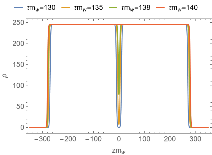
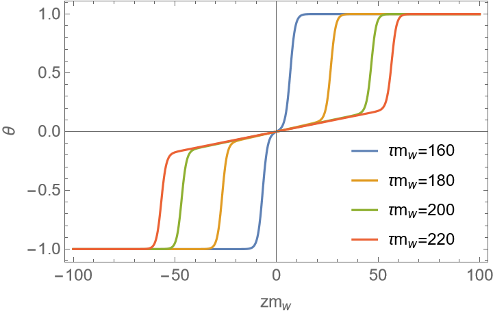
Figure 1: Left: Parameterized form for the scalar field of two colliding bubbles expending about their centers and coalescing Eq. (5) in the case of $t_{col}m_{\rm w}=200$; Right: We solve the Eq. (3) numerically, Higgs phase $\Theta$ is the field is shown as a the function of distance z along the axis of collision for $\tau m_{\rm w}=160,180,200,220$, with $\Theta_{0}=1$.

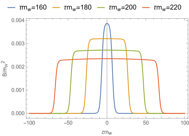
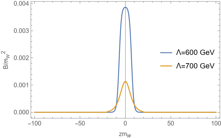
Figure 2: Left: The strength of the MFs as a function of the distance $z$ along the axis of collision at $\tau m_{\rm w}=160,180,200,220$ when $v_{\rm w}=0.7,\leavevmode\nobreak\ l_{\rm w}=0.025,\leavevmode\nobreak\ \Lambda=600$ GeV. Right: The strength of the MFs at $\tau m_{\rm w}=160$ for $\Lambda=600$ GeV, and $v_{\rm w}=0.33,\leavevmode\nobreak\ l_{\rm w}=0.048$ for $\Lambda=700$ GeV.

Then, the $j_{\nu}^{em}(x)$ as presented in Eq. (54) take the form

$$j_{\nu}^{em}(x)=(j_{z}(\tau,z),x_{\alpha}j(\tau,z)).$$ (6)

Where

$$j_{z}(\tau,z)=-(\frac{c_{1}}{g}+c_{2})\frac{8\rho(x)((\nabla_{z}\times\vec{E}_{1}))}{\Lambda^{2}}-\frac{g^{\prime}}{c_{2}}\rho{(x)}^{2}\frac{\partial\Theta(\tau,z)}{\partial z},$$ (7)

$$j(\tau,z)=-(\frac{c_{1}}{g}+c_{2})\frac{8\rho(x)\frac{\partial\rho(x)}{\partial\tau}B_{1}}{\Lambda^{2}}-\frac{g^{\prime}}{c_{2}}\rho{(x)}^{2}\frac{1}{\tau}\frac{\partial\Theta(\tau,z)}{\partial\tau}.$$

and $x_{\alpha}=(v_{\rm w}t,-x,-y)$. The electromagnetic field is similar in form to the electromagnetic current.

$$A_{\nu}^{em}=(a_{z}(\tau,z),x_{\alpha}a(\tau,z)),$$ (8)

By taking the axial gauge, Maxwell’s equations become

$$-\frac{\partial^{2}a(\tau,z)}{\partial z^{2}}=j(\tau,z),$$ (9)

By applying the boundary conditions, specifically: $a(\tau_{0},z)=0$, and $\partial_{z}a(\tau=0,z)=0$, we have

$$a(\tau,z)=-\int_{-\infty}^{z}dz^{\prime}\int_{-\infty}^{z^{\prime}}j(\tau,z)dz^{\prime\prime}.$$ (10)

Then, applying Eq. (56). Finally, we have determined the numerical value of the magnetic field resulting from bubble collisions in Fig. 2.

III Magnetic fields Evolution and baryogenesis

In this section, we first investigate the MF evolution with the MF produced during EWPT. And, we will further study the helical magnetic field effects on the lepton asymmetry and baryon asymmetry generation.

III.1 MF evolution without chiral anomaly

After the magnetic field is generated at PT, the qualitative picture of the evolution of magnetic fields and the primordial plasma is governed by the magnetohydrodynamic(MHD) equations. We first consider the scenario without Lepton asymmetry, in this case, the MHD equations read,

$$\frac{\partial{\bf B}}{\partial\eta}=-\nabla\times{\bf E},\leavevmode\nobreak\ \frac{\partial{\bf E}}{\partial\eta}+{\bf J}=\nabla\times{\bf B},$$ (11)

$${\bf J}=\sigma({\bf E}+{\bf v}\times{\bf B}),\nabla\cdot{\bf B}=0,\nabla\cdot{\bf E}=0.$$

Where, the conformal time is $\eta=M_{0}/T$, with $M_{0}=(90/8\pi^{3}g_{\star})^{1/2}M_{pl}$, $M_{pl}$ is the reduced Planck mass, and $g_{\star}\approx 106.75$. The current ${\bf J}$ is denoted as $\vec{j}^{em}$ in Eq. (56), ${\bf v}$ is the fluid velocity of the plasma and $\sigma=70T$ [53] is its conductivity. Neglecting the $\partial_{\eta}\bf E$ term, which remains small in the MHD approximation, so from Eq. (11) we can obtain

$$\frac{\partial\bf B}{\partial\eta}=\nabla\times({\bf v}\times{\bf B})+\frac{1}{\sigma}\nabla^{2}{\bf B}.$$ (12)

where ${\bf v}\times{\bf B}$ is the coupling term of plasma and magnetic field, which vanishes without vorticity.

Choosing the simplest nontrivial configuration of the magnetic field, which is

$$Y_{x}=Y(t)\sin k_{0}z,\leavevmode\nobreak\ Y_{y}=Y(t)\cos k_{0}z$$ (13)

$$Y_{z}=Y_{0}=0,$$

Thus the simple choice of wave configuration we obtain

$$(\nabla\times{\bf B})\cdot{\bf B}=k_{0}B(t)^{2},\leavevmode\nobreak\ {\bf B}=\nabla\times{\bf Y},$$ (14)

$${\bf B}^{2}=B(t)^{2},\leavevmode\nobreak\ \nabla^{2}{\bf B}=-k_{0}^{2}B(t),$$

where, $B(t)=k_{0}Y(t)$ is the magnetic field amplitude, and $k_{0}$ is the maximum wave number surviving Ohmic dissipation. Finally, we solve Eq. (12)

$$B(T)\simeq B_{0}\exp(\frac{-k_{0}^{2}M_{0}}{210T^{3}}).$$ (15)

where $B_{0}$ are the initial values of the magnetic field given by Eq. (56), and $T=100$ GeV is the initial temperature.

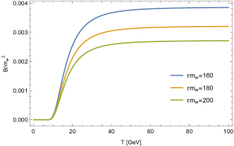
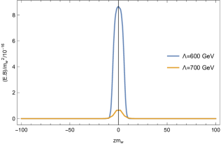
Figure 3: We obtain the numerical solution of Eq. (15) in units of $m_{\rm w}^{2}$. Left: The evolution of the magnetic field with temperature from 100 GeV to 150 MeV when $k_{0}=10^{-6}$, $\Lambda=600$ and the initial values for $\tau m_{\rm w}=160,\leavevmode\nobreak\ 170,\leavevmode\nobreak\ 180$. Right: CP violation as a function of the distance z along the axis of collision from the axis of collision at $\tau m_{\rm w}$ = 160 for $\Lambda$ = 600 GeV, 700 GeV.

The MF helicity is defined as the volume integral

$$\mathcal{H}\equiv\int_{V}d^{3}x{\bf A}\cdot{\bf B}\;.$$ (16)

with ${\bf A}$ being the vector potential and ${\bf B}\equiv\nabla\times{\bf A}$. The helical density of the MF is given by $h=<{\bf A}\cdot{\bf B}>$. The time derivative of the helicity density is [46]

$$\dot{h}=\lim_{V\rightarrow\infty}\frac{2}{V}\int_{V}d^{3}x\epsilon_{ijk}\dot{A_{i}}\partial_{j}A_{k}=-a^{2}\frac{2}{\sigma}<{\bf B}\cdot(\nabla\times{\bf B})>\simeq a^{3}\frac{4\pi}{\sigma}\frac{B^{2}}{\lambda_{B}},$$ (17)

where

$$\lambda_{B} \simeq v_{A}t\simeq\frac{B}{2H}\sqrt{\frac{3}{4\rho_{ch}}}=\frac{45BM_{pl}/T^{4}}{2\pi^{2}\sqrt{g_{\star}^{tot}g_{\star}^{ch}}}\;.$$ (18)

The magnetic field is obtained from Eq. (56), $\lambda_{B}$ is the physical length of the magnetic field with $g_{\star}^{tot}$ and $g_{\star}^{ch}$ being the number of degrees of freedom of all the particles in the thermal bath and the charged particles $U(1)$, respectively. We present the evolution of the MF helicity density directly calculated from the numerical solution of Eq. (17).

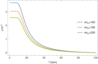
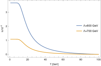
Figure 4: We show the temperature evolution of the total electromagnetic helicity (top panel). Left: Concerning the temperature for various initial values for $\tau m_{\rm w}=160,\leavevmode\nobreak\ 180,\leavevmode\nobreak\ 200$. Right: About temperature for $\Lambda=600$ GeV, 700 GeV.

The density of the Chern-Simons number $n_{CS}$ after the EWPT can be calculated to be [37]:

$$\bigtriangleup{n_{CS}}=-\frac{g^{\prime 2}}{2\pi^{2}}\int_{t_{0}}^{t_{\rm EW}}{\bf E}\cdot{\bf B}dt,$$ (19)

Because the phase transition is strongly first-order, the Chern-Simons number released before the EWPT will not be destroyed by the sphaleron process. This is because after the electroweak symmetry breaking, due to the appearance of the Higgs field, this process is suppressed [54]. Therefore, the baryon number $\eta_{B}$ is

$$\eta_{B}=\frac{3}{2s}\bigtriangleup{n_{CS}}\;,$$ (20)

where $s=\frac{2\pi^{2}g_{\star}^{2}T^{3}}{45}$ is the entropy density. In Fig. 5, we show that one cannot obtain an observable BAU solely considering the effect of the helical MF during post-EWPT evolution. In the next section, we propose to extend the system of MHD equations to incorporate the effect of the chiral anomaly for lepton currents after the EWPT.

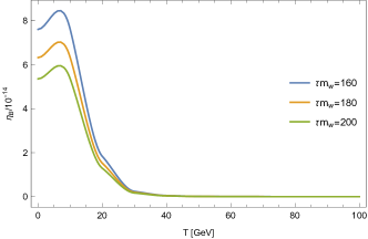
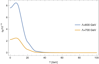
Figure 5: The two figures above are the numerical solution of Eq. (33), and the magnetic field also in units of $m_{\rm w}^{2}$. Left: The baryonic number $\eta_{B}$ as a function of temperature for $\Lambda=600$ GeV, and various initial values for $\tau m_{\rm w}=160,\leavevmode\nobreak\ 170,\leavevmode\nobreak\ 180$. Right: The baryonic number $\eta_{B}$ as a function of temperature for different various initial values of $\Lambda=600$, 700 GeV.

III.2 Baryogenesis from helical MF through chiral anomaly

The appearance of the helical MF leads to a change of the average number density of the left and right chiral electrons $n_{L}-n_{R}$ through the quantum effect of chiral anomaly [45]:

$$\frac{d(n_{L}-n_{R})}{dt}=-\frac{2\alpha}{\pi}\frac{1}{V}\int{\bf E}\cdot{\bf B}d^{3}x=\frac{\alpha}{\pi}\frac{d\mathcal{H}}{dt},$$ (21)

where $\alpha$ is the fine-structure constant, $n_{L,R}=\mu_{L,R}T^{2}/6$. Therefore, we can rewrite Eq. (21) as

$$\frac{d\Delta\mu}{dt}=-\frac{6\alpha}{\pi T^{2}}\frac{d\mathcal{H}}{dt}\;.$$ (22)

with $\Delta\mu=\mu_{R}-\mu_{L}$ is the difference between right and left chemical potentials. The chiral anomaly leads to an additional contribution to the current in Maxwell’s equations

$$\leavevmode\nobreak\ \frac{\partial{\bf E}}{\partial t}+{\bf J}+\frac{\alpha\Delta\mu(t){\bf B}}{\pi}=\nabla\times{\bf B},\leavevmode\nobreak\ {\bf J}=\sigma{\bf E}+{\bf v}\times{\bf B},$$ (23)

$$\frac{\partial{\bf B}}{\partial t}=-\nabla\times{\bf E},\leavevmode\nobreak\ \nabla\cdot{\bf E}=0,\leavevmode\nobreak\ \nabla\cdot{\bf B}=0,$$

Neglecting the displacement current, $\partial_{t}{\bf E}$, which remains small in the approximation. In our work, we neglect the effects of fluid velocity, deferring the broader question of the interaction between turbulence and chiral asymmetry to future research. From Eq. (23), we obtain:

$$\frac{\partial B}{\partial t}=\frac{\alpha}{\pi}\frac{\Delta\mu}{\sigma}\nabla\times B+\frac{1}{\sigma}\nabla^{2}B.$$ (24)

We assume that the fields are slowly varying and neglect the effects depending on the velocity field. Similarly, we use conformal quantities to explain the evolution of the magnetic field in an expanding universe. From Eq. (24) we can obtain the evolution equations for the real binary products in the Fourier space, with $\rho_{B}(\eta)=\int dk\rho_{k}(k,\eta)=B(\eta)^{2}/2$ is the magnetic energy density and $\mathcal{H}(\eta)=\int dk\mathcal{H}_{k}(k,\eta)$ is the magnetic helicity density, and satisfy the inequality $\rho_{B}(\eta)\geq k|\mathcal{H}_{k}(\eta)|/2$, which becomes saturated for field configurations termed maximally helical fields $\rho(k,\eta)=k|\mathcal{H}_{k}(k,\eta)|/2$ given by $\rho_{B}(\eta)=B(\eta)^{2}/2$. For convenience, When we discuss $k$ in the following sections, $k$ represents the conformal form.

The general system of evolution equations for the spectra of the helicity density $\mathcal{H}_{k}(k,\eta)$ and the energy density $\rho_{B}(k,\eta)$ in the conformal coordinates reads [30]

$$\frac{d\rho_{B}(k,\eta)}{d\eta}=-\frac{2k^{2}}{\sigma}\rho_{B}(k,\eta)+\frac{\alpha\Delta\mu k^{2}}{2\pi\sigma}\mathcal{H}_{k}(k,\eta),$$ (25)

$$\frac{d\mathcal{H}_{k}(k,\eta)}{d\eta}=-\frac{2k^{2}}{\sigma}\mathcal{H}_{k}(k,\eta)+\frac{2\alpha\Delta\mu}{\pi\sigma}\rho_{B}(k,\eta),$$

$$\frac{d\Delta\mu(\eta)}{d\eta}=-\frac{6\alpha}{\pi}\int dk\frac{\partial\mathcal{H}_{k}(k,\eta)}{\partial\eta}-\Gamma_{f}\Delta\mu(\eta),$$

Where $\Gamma_{f}$ is the chirality flip rate, and instead of Higgs inverse decays, the dominant contribution to chirality flips now comes from weak and electromagnetic scattering processes. Although the chirality flipping rate $\Gamma_{f}$ is suppressed compared to the rate of chirality preserving weak and electromagnetic processes, it is still faster than the Hubble expansion rate $H(T)$. Therefore, we need to take chirality flipping processes into account at lower temperatures, So we obtain [55]:

$$\Gamma_{em}\simeq 1.17\times\alpha\frac{m_{e}^{2}}{T}\,\qquad \Gamma_{{\rm w}}\simeq G_{F}^{2}T^{5}(\frac{m_{e}}{3T})^{2}\;.$$ (26)

Where, $G_{F}$ is the Fermion constant, both chirality flipping rates in the broken phase are given by $\Gamma_{f}=\Gamma_{em}+\Gamma_{\rm w}$. Here, we do not consider the sphaleron effect because it is suppressed after the electroweak phase transition in Ref. [51]

The solution of the second equation in Eq. (25) takes the form:

$$\mathcal{H}_{k}(k,\eta)=\mathcal{H}_{k}(k,\eta_{0})\exp(\frac{2k}{\sigma}(\frac{\alpha}{2\pi}\int_{\eta_{0}}^{\eta}\Delta\mu(\eta^{\prime})d\eta^{\prime}-k(\eta-\eta_{0}))),$$ (27)

where $\mathcal{H}_{k}(k,\eta_{0})$ is helical magnetic field initial spectrum, and initial conditions at the time $\eta_{0}=7\times 10^{15}$ when the EWPT occurs. For convenience, one can use the notation of

$$\mathcal{H}_{k}(k,\eta)=\mathcal{H}_{k}(k,\eta_{0})\exp(A(\eta)k-B(\eta)k^{2})\;,$$ (28)

with

$$A(\eta)=\frac{\alpha}{\sigma\pi}\int_{\eta_{0}}^{\eta}\Delta\mu(\eta^{\prime})d\eta^{\prime},\leavevmode\nobreak\ B(\eta)=\frac{2}{\sigma}(\eta-\eta_{0})\;.$$ (29)

For the continuous spectrum, the helicity density is therefore obtained as,

$$\mathcal{H}_{k}(\eta)=\int_{k_{min}}^{k_{max}}\mathcal{H}_{k}(k,\eta)dk$$ (30)

For the initial spectrum $\mathcal{H}_{k}(k,\eta_{0})=Ck^{n_{s}}=2\rho(k,\eta_{0})/k$ with $n_{s}\geq 3$, the $\Delta\mu$ will decay more slowly, and the constant C can be estimated using the relation for the full helical field. Using the initial magnetic field energy density formula $\rho_{B}(\eta_{0})=\int\rho_{B}(k,\eta_{0})dk=B_{0}^{2}/2$, we obtain

$$C=\frac{2\rho_{B}^{2}(\eta_{0})(n_{s}+2)}{k_{max}^{n_{s}+2}-k_{min}^{n_{s}+2}}\;.$$ (31)

For $k\rightarrow 0$ violates the causal lower limit, $k>k_{min}=l_{H}^{-1}=10^{-16}$ at $T\sim 100$ GeV, $k_{max}$ is an arbitrary wave number parameter constrained by the conditions previously discussed. Therefore, we will ignore the $k_{min}$ term in the following calculations. Meanwhile, the last section suggests that the initial magnetic energy density $\rho_{B}(\eta_{0})=\frac{B_{0}^{2}}{2}\simeq 3\times 10^{-6}$ and $\xi_{e}(\eta_{0})=\Delta\mu(\eta)/T\simeq 10^{-12}$. Finally, the helicity density for the continuous spectrum is obtained as [42]:

$$\mathcal{H}_{k}(\eta)=C\int_{0}^{k_{max}}k^{n_{s}}\exp(A(\eta)k-B(\eta)k^{2})dk\;.$$ (32)

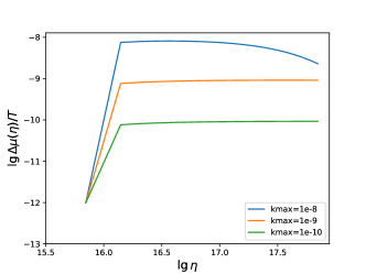
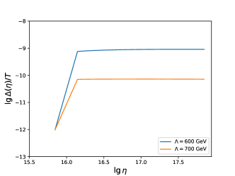
Figure 6: The evolution of the chemical potential in logarithmic scale for the continuous spectrum and $n_{s}=3$. Left: the growth of the chemical potential for the initial value $\Delta\mu(\eta_{0})=10^{-10}$ for the different wave number $k_{max}=10^{-8},\leavevmode\nobreak\ 10^{-9},\leavevmode\nobreak\ 10^{-10}$. Right: the growth of the chemical potential for $\Lambda=600$ GeV, 700 GeV when $k_{max}=10^{-9}.$

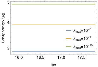
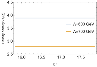
Figure 7: Conservation of the magnetic field helicity density for continuous spectrum $\mathcal{H}_{k}(k,\eta_{0})\propto k^{3}$. Left: the approximation of the spectrum by different $k_{max}=10^{-8},\leavevmode\nobreak\ 10^{-9},\leavevmode\nobreak\ 10^{-10}$. Right: helicity density with conformal time for $\Lambda=600$ GeV, 700 GeV when $k_{max}=10^{-9}$.

We numerically solved the system equations of Eqs. (25). In Fig. 6, We demonstrate the evolution of the asymmetry difference between left-handed and right-handed leptons $\Delta\xi_{e}(\eta)=\xi_{eR}(\eta)-\xi_{eL}(\eta)$, which is the import initial parameter for the chiral magnetic effect after the EWPT, $\Delta\xi_{e}(\eta_{EW})=\Delta\mu(\eta_{EW})/T$ [30]. The growth of $\Delta\xi_{e}(\eta)$ due to the Abelian anomaly and its tendency to reach a constant value is obtained in [42], particularly in the context of a monochromatic helicity density spectrum. Here, we obtain a similar time independence of the saturation values of $\Delta\xi_{e}(\eta)$ for a continuous helicity density spectrum. As indicated in the left Fig. 7, in the case of the continuous spectrum $n_{s}=3$ the helicity density $\mathcal{H}_{k}(\eta)$ is almost conserved for the fully helical case at lower $k>k_{min}=l_{H}^{-1}=10^{-16}$. On the right panel, we demonstrate the conservation values of different helical densities corresponding to various new physical scales for $k_{max}=10^{-9}$.

We now discuss the generation of the BAU. After considering ’t Hooft’s conservation law $\eta_{B}(t)/3-L_{e}(t)=$ const ( $\eta_{B}=(n_{B}-n_{\bar{B}})/s$ and $L_{l}=(n_{l}-n_{\bar{l}})/s$ are the baryon and lepton numbers correspondingly), and, Thus [44],

$$\frac{\partial(n_{B}-n_{\bar{B}})/s}{\partial t}=\frac{3g^{\prime 2}}{8\pi^{2}s}{\bf E}\cdot{\bf B};,$$ (33)

Combining with the third equation of Eq. 25, comparing the result with Eq. 33, and in conformal variables, we have

$$\eta_{B}(\eta)=\int_{\eta_{0}}^{\eta}-\frac{135g^{\prime 2}}{32\pi^{4}g_{\star}}\frac{d\mathcal{H}(\eta^{\prime})}{d\eta^{\prime}}d\eta^{\prime}\;.$$ (34)

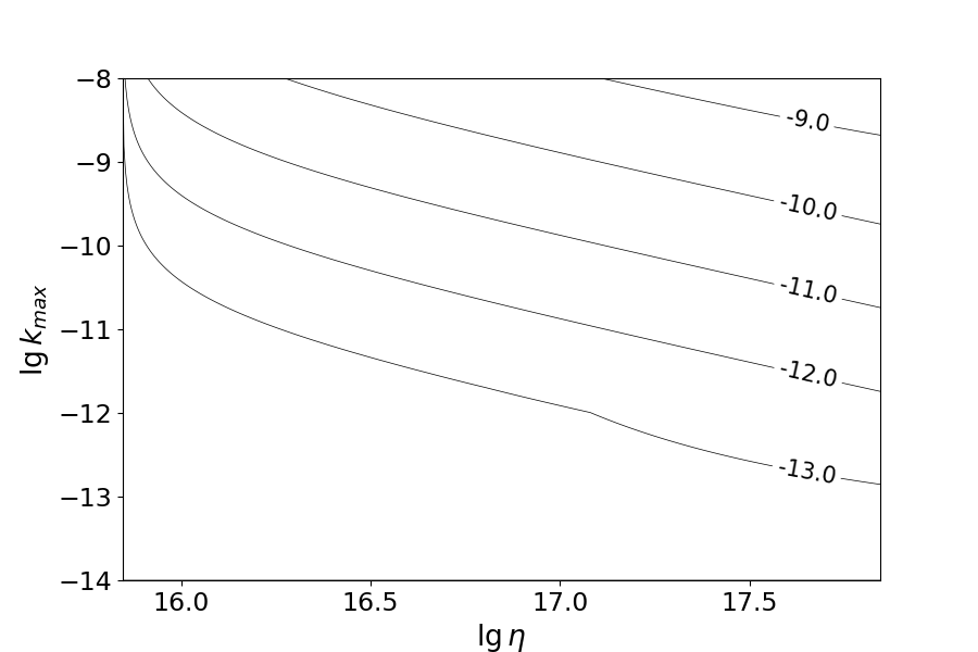
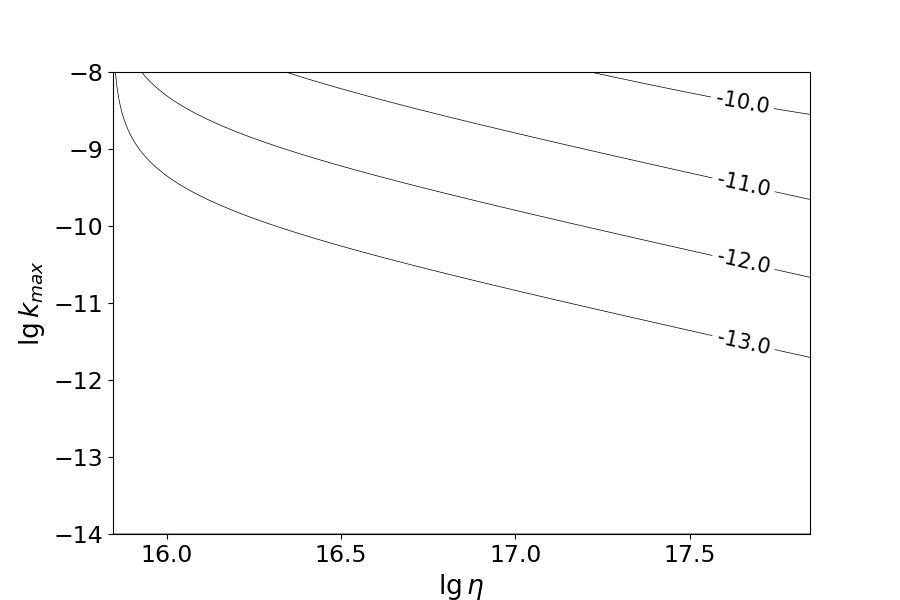
Figure 8: The two figures above are the numerical solution of Eq. (25) and Eq. (34), the baryon asymmetry of university evolution after EWPT is dependent on the conformal time $\eta$ and different larger wave numbers value $k_{max}$ for the continuous spectrum ($n_{s}=3$). Left: $\Lambda=600$ GeV. Right: $\Lambda=700$ GeV.

In Fig. 8, we show the growth of the BAU driven by the chiral asymmetry in the electromagnetic field. The growth of positive BAU with the increase of $k_{max}$ and the conformal time $\eta$ is the generic feature. We have provided a clearer representation of the range of $k_{max}$ values, from the minimum to the maximum, where the BAU can reach the observed value $\eta_{B}\sim 10^{-10}$ with different energy scales of new physics of $\Lambda=600$ GeV and $\Lambda=700$ GeV.

IV Cosmological observation of the Magnetic field

Here, we briefly discuss cosmic observations for these MF generated during the EWPT. Since the phase transition type is of first-order, its correlation scale which is of the order of the size of mean bubble separation at coalescence, which is of the order of comoving correlation length $\lambda\simeq 0.01l_{H}$ [20], $l_{H}$ denotes the comoving Hubble scale being given by [56]:

$$l_{H}=5.8*10^{-10}{\rm Mpc}(100{\rm GeV}/T)(100/g_{\star})^{1/6}\;,$$ (35)

where $T$ is at the electroweak phase transition temperature. The physical magnetic field amplitudes scale with the expansion of the universe as

$$B_{\star}=(\frac{a_{\star}}{a_{0}})^{2}B(T)\;,$$ (36)

where $B(T)$ is given by Eq. (15), with the time-temperate relation being [57]:

$$\frac{a_{\star}}{a_{0}}\simeq 8*10^{-16}(100{\rm GeV}/T)(100/g_{\star})^{1/3}\;,$$ (37)

which is the ratio of the scale factor at the time of MF generation to that at present. The simulation of the evolution of hydromagnetic turbulence from the EWPT until today suggests that the root-mean-squared (nonhelical and helical) MF amplitude and the correlation length satisfy the following relation [57]:

$$B_{rms}=B_{\star}(\lambda_{B}/\lambda)^{-(\beta+1)/2}\;.$$ (38)

Where, $\beta=0$ is for the helical MF case, $\beta=1,2$ for the non-helical MF case, and the fractionally helical MF case with $\epsilon_{M}=10^{-3}$ [57], and $\lambda_{B}$ is the correlation length. As studied in previous sections, the generated MF during the EWPT under study will reach a fully helical case, and cannot be probed currently, see Fig. 9.

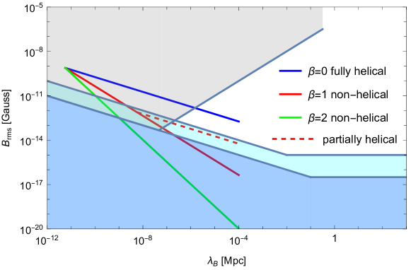
Figure 9: MF strength $B_{rms}$ versus the correlation length $\lambda_{B}$ for the fully helical case (blue), fractionally helical case (red dash lines), and non-helical case (red and green). The gray region shows the upper bound on the MF strength considering the MHD evolution [58, 59], the cyan and blue regions are plotted to consider the bounds set by the Blazars given in Refs.[60, 58].

V Conclusion

We perform a thorough study of the the generation from the helical MF to the baryon asymmetry of the Universe. We utilize the model of the SM extended by dimension-six operators, where the CP-even operator ensures bubble collision occurs during the first-order EWPT, and the MF generated during bubble collision is found to be helical when the assistant of the CP-odd operator appears. The helical MF can induce the Chern-Simons number change and produce the baryon number, while the generated baryon asymmetry is far smaller than the observed BAU. We further demonstrate that the evolution of magnetic fields in a primordial plasma containing Standard Model particles is strongly affected by the quantum chiral anomaly. As a result, this leads to the generation of lepton asymmetry which is proportional to the new physics scale. When the new physics scale $\Lambda\lesssim 700$ GeV, the generated lepton asymmetry can reach $\Delta\mu/T\gtrsim 10^{-10}$ and therefore ensure enough generation of the baryon number to explain the BAU puzzle. This is the first time to study the baryogenesis by providing a specific source of the MF rather than hypothesizing about the origin and magnitude of the magnetic field. Meanwhile, we observe that only for large wavenumbers $k_{max}\leavevmode\nobreak\ (k_{max}\gtrsim 10^{-10})$ of the MF helicity density does the baryon asymmetry grow significantly and exceed the observable BAU value of $\eta_{B}\sim 10^{-10}$.

VI Acknowledgements

This work is supported by the National Key Research and Development Program of China under Grant No. 2021YFC2203004. L.B. is supported by the National Natural Science Foundation of China (NSFC) under Grants Nos. 12075041, 12147102, 12322505. L.B. also acknowledges Chongqing Natural Science Foundation under Grant No. CSTB2024NSCQ-JQX0022 and Chongqing Talents: Exceptional Young Talents Project No. cstc2024ycjh-bgzxm0020.

Appendix A Equation of motions

This Lagrangian under study is of the form:

$$L_{EW}=L_{1}+L_{2}-V(\phi)+c_{6}\phi^{\dagger}\phi B_{\mu\nu}\tilde{B}^{\mu\nu}$$ (39)

with

$$L_{1}=-\frac{1}{4}W_{\mu\nu}^{i}W^{i\mu\nu}-\frac{1}{4}B_{\mu\nu}^{i}B^{i\mu\nu}$$

$$W_{\mu\nu}^{i}=\partial_{\mu}W_{\nu}^{i}-\partial_{\nu}W_{\nu}^{i}-g\epsilon_{ijk}W_{\mu}^{j}W_{\nu}^{k}$$

$$B_{\mu\nu}=\partial_{\mu}B_{\nu}-\partial_{\nu}B_{\nu}$$

$$L_{2}=|i\partial_{\mu}-\frac{g}{2}\tau\cdot W_{\mu}-\frac{g^{\prime}}{2}B_{\mu}\Phi|$$ (40)

$$V(\phi)=\mu_{h}^{2}\Phi^{\dagger}\Phi+\lambda(\Phi^{\dagger}\Phi)^{2}+c_{6}(\Phi^{\dagger}\Phi)^{3}$$

where the $W^{i}$, with ${i=(1,2)}$, are the $W^{\pm}$fields, the $U(1)_{Y}$ hypercharge gauge field $B_{\mu}$, $\Phi$ is the Higgs field, $\tau^{i}$is the SU(2) generator, $B_{\mu\nu}$ is electromagnetic field strength tensor, $c_{6}=\Lambda^{-2}$ and $\tilde{B}^{\mu\nu}$ is the dual tensor, and $\Lambda$ is the energy scale of new physics that suppresses the dimension-six CP-violating operator. The electromagnetic field strength tensor is given:

$$B^{\mu\nu}=\begin{pmatrix}0&E_{x}&E_{y}&E_{z}&\\ -E_{x}&0&-B_{z}&-B_{y}&\\ -E_{y}&-B_{z}&0&B_{x}&\\ -E_{z}&B_{y}&-B_{z}&0&\end{pmatrix}$$

And, the electromagnetic and Z fields are defined as

$$A_{\mu}^{EM}=\frac{1}{\sqrt{g^{\prime 2}+g^{2}}}(g^{\prime}W_{\mu}^{3}+gB_{\mu})$$ (41)

$$Z_{\mu}=\frac{1}{\sqrt{g^{\prime 2}+g^{2}}}(gW_{\mu}^{3}-g^{\prime}B_{\mu})$$ (42)

The effective Higgs potential $V(\Phi)$ is not relevant to this paper. $g=\frac{e}{\sin(\theta_{w})}=0.646,g^{\prime}=g\tan(\theta_{w})=0.343$, and the paper units are such that $\hbar=c=1$. Equations of motion from the Lagrangian given by Eq. (39) can be obtained by applying the principle of least action $\delta\int d^{4}xL_{EW}=0$. The modulus $\rho$ of the Higgs field satisfies the $\rho$-equation

$$0 =\partial^{2}\rho(x)-\frac{g^{2}}{4}\rho(x)[{W}^{1}\cdot{W}^{1}+{W}^{2}\cdot{W}^{2}]-\rho(x)\psi_{\nu}\psi^{\nu}+\rho(x)\frac{\partial V}{\partial\rho^{2}}-\frac{\rho(x)B_{\mu\nu}\tilde{B}^{\nu\mu}}{\Lambda^{2}}$$ (43)

Where the quantity $\psi_{\nu}$ is defined in terms of the phase of the Higgs field and the Z field. The B field satisfies a $B$-equation.

$$\partial^{2}B_{\nu}-\partial_{\nu}\partial\cdot B+g^{\prime}\rho(x)^{2}\psi_{\nu}(x)=\frac{4\partial^{\mu}(\rho(x)^{2})\tilde{B}_{\nu\mu}}{\Lambda^{2}}\;,$$ (44)

where the $\psi_{\nu}$ is

$$\psi_{\nu}(x)\equiv\partial_{\nu}\Theta-\frac{\sqrt{g^{2}+g^{\prime 2}}}{2}Z_{\nu}\;,$$ (45)

and satisfies

$$\partial^{\nu}\left(\rho(x)^{2}\psi_{\nu}(x)\right)=0\;.$$ (46)

For $i=3$, gauge field $W^{i}$ satisfies the following $W$-equation

$$\partial^{2}W^{3}_{\nu}-\partial_{\nu}\partial\cdot W^{3}-g\rho(x)^{2}\psi_{\nu}(x)=j^{3}_{\nu}(x)\;,$$ (47)

and, for $i=1,2$, we have

$$\partial^{2}W^{i}_{\nu}-\partial_{\nu}\partial\cdot W^{i}+m_{W}(x)^{2}W^{i}_{\nu}=j^{i}_{\nu}(x)\;,$$ (48)

with $m_{W}(x)^{2}=g^{2}\rho(x)^{2}/2$, and $j^{i}_{\nu}(x)$ is,

$$j^{i}_{\nu}(x)\equiv g\epsilon_{ijk}(W^{k}_{\nu}\partial\cdot W^{j}+2W^{j}\cdot\partial W^{k}_{\nu}-W^{j}_{\mu}\partial_{\nu}W^{k\mu})-g^{2}\epsilon_{klm}\epsilon_{ijk}W^{j}_{\mu}W^{l\mu}W^{m}_{\nu}\;.$$ (49)

The EOM for $A^{em}$ casts the form of,

$$\partial^{2}A^{em}_{\nu}-\partial_{\nu}\partial\cdot A^{em}=j^{em}_{\nu}(x)\;,$$ (50)

with

$$c_{1}=\frac{g^{\prime}}{\sqrt{g^{2}+g^{\prime 2}}},\leavevmode\nobreak\ \leavevmode\nobreak\ c_{2}=\frac{g}{\sqrt{g^{2}+g^{\prime 2}}}$$ (51)

$$j^{em}_{\nu}(x)=c_{1}\times j^{3}_{\nu}(x)+c_{2}\times\frac{4\partial^{\mu}(\rho(x)^{2})\tilde{B}_{\nu\mu}}{\Lambda^{2}}\;.$$

And, the EOM for the $Z$ field is obtained as,

$$\partial^{2}Z_{\nu}-\partial_{\nu}\partial\cdot Z-\rho(x)^{2}\sqrt{g^{2}+g^{\prime 2}}\psi_{\nu}(x)-c_{2}\times j_{\nu}^{3}+\frac{4c_{1}}{\Lambda^{2}}\partial^{\mu}(\rho(x)^{2})\tilde{B}_{\nu\mu}=0\;.$$ (52)

Utilizing the thermal erasure [61] of $\langle Z\rangle=0$. Applying the ensemble averaging to Eq. (50), we can obtain

$$\langle j^{em}_{\nu}\rangle=(\frac{c_{1}}{g}+c_{2})\frac{4\partial^{\mu}(\rho(x)^{2})\tilde{B}_{\nu\mu}}{\Lambda^{2}}-\frac{g^{\prime}}{c_{2}}\rho{(x)}^{2}\times\partial_{\nu}\Theta(x)\;$$ (53)

Consequently, the Eq. (50) recasts the form of the Maxwell equation,

$$\partial^{2}A_{\nu}-\partial_{\nu}\partial\cdot A=j_{1}(x)+j_{2}(x)$$ (54)

where

$$j_{1}(x)=-(\frac{c_{1}}{g}+c_{2})\frac{8\rho(x)(\frac{\partial\rho(x)}{\partial t}{\vec{B}_{1}}+(\nabla\rho(x))\times{\vec{E_{1}}})}{\Lambda^{2}}, j_{2}(x)=-\frac{g^{\prime}}{c_{2}}\rho{(x)}^{2}\times\partial_{\nu}\Theta(x);$$ (55)

Specifically, ${\vec{B}_{1}}$ and ${\vec{E}_{1}}$ from magnetic field tensor $B^{\mu\nu}$, with its magnitude determined by the contribution of Higgs phase $\theta(x)$ from the current $j_{2}(x)$. Due to the magnetic field $\vec{B}=\vec{\nabla}\times\vec{A}^{em}$. When the Higgs fields of the colliding bubbles differ in phase before the collision, $\partial_{\nu}\Theta(x)$ develops a non-zero value within the bubble overlap region after the collision. The electromagnetic current $j^{em}_{\nu}(x)$ then develops a non-zero value there and magnetic fields will form. So we can calculate the strength of the magnetic field after obtaining the electromagnetic current through and the magnetic field in units of $m_{w}^{2}$

$$\nabla^{2}\vec{B}=\vec{\nabla}\times\vec{j}^{em}\;.$$ (56)

Appendix B Chern-Simons density

We study the Chern-Simons density in the Standard Model Effective Theory with the dimensional reduction (DR) in this part. The original $4d$ Lagrangian is given in Eq. (39). The operator $\Phi^{{\dagger}}\Phi B_{\mu\nu}\tilde{B}^{\mu\nu}$ will change the wave function renormalization, but this change is at order $\mathcal{O}(g^{4})$ due to the power counting $c_{6}\sim g^{4}/\Lambda^{2}$ [51]. This leads to a higher order than $\mathcal{O}(g^{4})$ in the 3d coupling matching, and it should be ignored in the study of phase transition dynamic. After integrating out super heavy mode, the effective theory has the form [51, 62]

$$\mathcal{L}^{heavy}_{3d}=\frac{1}{4}W_{ij}^{a}W_{ij}^{a}+\frac{1}{4}B_{ij}B_{ij}+\frac{1}{2}(D_{i}W_{0}^{a})^{2}+\frac{1}{2}(\partial_{i}B_{0})^{2}+\frac{1}{2}(D_{i}C_{0}^{\alpha})^{2}+(D_{i}\Phi)^{\dagger}(D_{i}\Phi)+V^{heavy}_{3d}\;,$$ (57)

where $W^{a}_{ij}=\partial_{i}W^{a}_{j}-\partial_{j}W^{a}_{i}+g_{3}\epsilon^{abc}W_{i}^{b}W_{j}^{c}$, $B_{ij}=\partial_{i}B_{j}-\partial_{j}B_{i}$ and $D_{i}\Phi=(\partial_{i}-ig_{3}\tau^{a}W_{i}^{a}/2-ig^{\prime}_{3}B_{i}/2)\Phi$ with $\tau^{a}$ being the Pauli matrices. The heavy scalar potential has the form

$$V^{heavy}_{3d}= \mu_{h,3}^{2}\Phi^{\dagger}\Phi+\lambda_{3}(\Phi^{\dagger}\Phi)^{2}+c_{6,3}(\Phi^{\dagger}\Phi)^{3}+\frac{1}{2}m_{D}^{2}\,W^{a}_{0}W^{a}_{0}+\frac{1}{2}m_{D}^{\prime 2}\,B_{0}^{2}+\frac{1}{2}m_{D}^{\prime\prime 2}\,C^{\alpha}_{0}C^{\alpha}_{0}$$ (58)

$$+\frac{1}{4}\kappa_{1}(W^{a}_{0}W^{a}_{0})^{2}+\frac{1}{4}\kappa_{2}B_{0}^{4}+\frac{1}{4}\kappa_{3}W^{a}_{0}W^{a}_{0}B_{0}^{2}+h_{1}\Phi^{\dagger}\Phi W^{a}_{0}W^{a}_{0}+h_{2}\Phi^{\dagger}\Phi B_{0}^{2}+\kappa_{0}B_{0}$$

$$+h_{3}B_{0}\Phi^{\dagger}{W}_{0}^{a}\tau^{a}\Phi+h_{4}\Phi^{\dagger}\Phi C^{\alpha}_{0}C^{\alpha}_{0}+\rho\Phi^{\dagger}W_{0}^{a}\tau^{a}\Phi+\rho^{\prime}\Phi^{\dagger}\Phi B_{0}+\rho_{G}B_{0}W_{0}^{a}W_{0}^{a}$$

$$+\alpha_{0}\epsilon_{ijk}\left(W_{i}^{a}W_{jk}^{a}-\frac{i}{3}g_{3}\epsilon^{abc}W_{i}^{a}W_{i}^{b}W_{k}^{c}\right)+\alpha^{\prime}\epsilon_{ijk}B_{i}B_{jk}\;,$$

where $m_{D},m_{D}^{\prime},m_{D}^{\prime\prime}$ are the Debye masses of the time component of gauge fields. The parameters of heavy scalar potential Eq. (58) are defined in Ref. [51]. The Chern-Simons terms $\alpha_{0}$ and $\alpha^{\prime}$ are defined as

$$\alpha_{0}=\frac{g^{2}}{32\pi^{2}}(N_{f}\mu_{B}+\sum_{i=1}^{3}\mu_{L_{i}}),\quad\alpha^{\prime}= -\frac{g^{\prime 2}}{32\pi^{2}}(N_{f}\mu_{B}+\sum_{i=1}^{3}\mu_{L_{i}})\;,$$ (59)

where the $N_{f}$ is the number of families, and $\mu_{B},\mu_{L_{i}}$ are the baryon and lepton chemical potential respectively. The relation $(N_{f}\mu_{B}+\sum_{i=1}^{3}\mu_{L_{i}})$ can be obtained by assuming the left- and right-hand fermion has the same chemical potential, and it vanished by defining [51] [62]

$$\mu_{B}=\frac{1}{N_{f}}\sum_{i=1}^{N_{f}}\mu_{i},\quad\mu_{L_{i}}=-\mu_{i}\;.$$ (60)

However, the lepton chemical potential is not equal to each other($\mu_{L_{i}}\neq\mu_{R_{i}}$) since the lepton asymmetry, where $\mu_{L_{i}}$ is the chemical potential of left-hand lepton and $\mu_{R_{i}}$ is the chemical potential of right-hand lepton. Then the Chern-Simons term with the lepton asymmetry has the form [63]

$$c_{E}\epsilon_{ijk}\biggr{(}W_{i}^{a}W_{jk}^{a}- \frac{i}{3}g_{3}\epsilon^{abc}W_{i}^{a}W_{i}^{b}W_{k}^{c}\biggr{)}+c_{E}^{\prime}\epsilon_{ijk}B_{i}B_{jk},$$ (61)

$$c_{E}=3N_{f}\mu_{B}+\sum_{i=1}^{N_{f}} \mu_{L_{i}},\quad c_{E}^{\prime}=-c_{E}+2\sum_{i=1}^{N_{f}}(\mu_{L_{i}}-\mu_{R_{i}}).$$ (62)

The rate of $B+L$ violation is significantly larger than the Hubble rate, and the system can pass over the barrier between the different vacua instead of penetrating through the barrier since the rate of the anomalous non-conservation of the fermion number can be unsuppressed in this system [63, 64]. For this reason, the abnormal processes are perfectly in thermal equilibrium, and the chemical potential should be set to zero $\mu_{B+L}=3N_{f}\mu_{B}+\sum_{i=1}^{N_{f}}\mu_{L_{i}}=0$ and $c_{E}$ vanishes.

But the $c_{E}^{\prime}$ does not vanish because the right-hand lepton($e_{R}$) is coupled with the $U(1)_{Y}$ hypercharge gauge field. This interaction does not change the quantum numbers or generation, while the Yukawa interaction can change the quantum numbers or generation. The Yukawa interaction between the Higgs and electron is very weak for the tiny electron mass. That leads to the $e_{R}$ coming into chemical equilibrium at temperature $T\simeq 1$ TeV. Since the sphaleron process falls out of equilibrium near this temperature, the $e_{R}$ may not be transformed into $e_{L}$ soon enough, and the initial $e_{R}$ asymmetry is not washed out [25, 65].

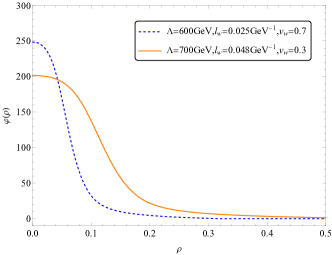
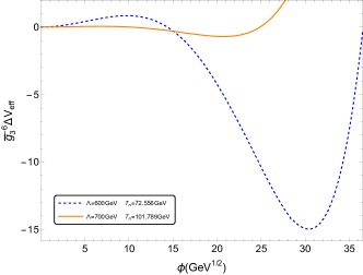
Figure 10: The initial bubble profiles (left) and the corresponding effective thermal potential at the nucleation temperature (right).

The Fig. 10 shows the effective potential $\Delta V_{eff}$ and bounce profile at temperature $T_{n}$ with the $\Lambda=600$ GeV and $700$ GeV. The $\Delta V_{eff}=V_{eff}(\phi)-V_{eff}(0)$ is calculated in light scale and has dimension GeV³, and $\overline{g}_{3}^{2}$ is the $SU(2)$ gauge coupling in the light scale with dimension GeV² [51]. The nucleation temperature $T_{n}$ is obtained when the bubble nucleation rate $\Gamma=A\exp[-S_{c}]$ is equal to Hubble parameter $\Gamma\sim H$, i.e., $S_{c}\approx 140$ [66]. The Euclidean action is

$$S_{c}=\int\bigg{[}\frac{1}{2}(\partial_{i}\phi)^{2}+V_{eff}(\phi,T)\bigg{]}d^{3}x.$$ (63)

The action can be obtained by solving the bounce function:

$$\frac{d^{2}\phi}{d\rho^{2}}+\frac{2}{\rho}\frac{d\phi}{d\rho}=\frac{dV_{eff}(\phi,T)}{d\phi}\;,$$ (64)

with the boundary condition

$$\phi(\rho\rightarrow\infty)=0,\quad\left.\frac{d\phi}{d\rho}\right|_{\rho=0}=0\;,$$ (65)

and we use code “findbounce” to solve this equation and obtain the nucleation temperature $T_{n}$ and the corresponding background field value $\phi_{n}$ [67]. The $l_{w}$ in SMEFT has the form [68]

$$l_{w}=\sqrt{\frac{\phi_{n}^{2}}{4V_{h}}},\quad V_{h}=\Delta V_{eff}^{max}-\Delta V_{eff}^{min},$$ (66)

where $V_{h}$ is the height of the potential barrier. The bubble wall velocity is defined as [68]

$$v_{w}=\begin{cases}\sqrt{\frac{\Delta V}{\alpha_{n}\rho_{r}}}&,\quad\sqrt{\frac{\Delta V}{\alpha_{n}\rho_{r}}}<v_{J}(\alpha_{n})\\ 1&,\quad\sqrt{\frac{\Delta V}{\alpha_{n}\rho_{r}}}\geq v_{J}(\alpha_{n})\end{cases}$$ (67)

with the $\Delta V$ being the difference between the broken phase and symmetric phase and the Jouguet velocity $v_{J}(\alpha_{n})$ is [68, 69]

$$v_{J}=\frac{1}{\sqrt{3}}\frac{1+\sqrt{3\alpha_{n}^{2}+2\alpha_{n}}}{1+\alpha_{n}}\;,$$ (68)

where $\alpha_{n}$ is the strength of phase transition.

We calculate the Chern-Simons density of $U(1)_{Y}$ gauge field $B_{\mu}$ with the configuration of gauge and Higgs fields

$$g^{\prime}B_{i}dx^{i} =(1-f_{0}(\xi))F_{3},$$ (69)

$$gW_{i}^{a}\tau^{a}dx^{i} =(1-f(\xi))(F_{1}\tau^{1}+F_{2}\tau^{2})+(1-f_{3}(\xi))F_{3}\tau^{3},$$

$$\phi =\frac{v(T)}{\sqrt{2}}\begin{pmatrix}0\\ h(\xi)\end{pmatrix},$$

where the function $F_{i}$’s are defined in Ref. [51]. The function $f(\xi),h(\xi),f_{0}(\xi)$ and $f_{3}(\xi)$ can be obtained by solve Eq. (70)

$$f^{\prime\prime}+\frac{1-f}{4\xi^{2}}\left[8\sin^{2}\nu(f(f-2)+f_{3}+f_{3}^{2})+\xi^{2}h^{2}\right]=0,$$ (70)

$$f^{\prime\prime}_{3}-\frac{2}{\xi^{2}}\sin^{2}\nu\left[3f_{3}+f(f-2)(1+2f_{3})\right]-\frac{h^{2}}{4}(f_{3}-f_{0})=0,$$

$$f^{\prime\prime}_{0}+\sin^{2}\nu\frac{g^{\prime 2}}{4g^{2}}h^{2}(f_{3}-f_{0})+2\frac{1-f_{0}}{\xi^{2}}=0,$$

$$h^{\prime\prime}+\frac{2}{\xi}h^{\prime}-\sin^{2}\nu\frac{2}{3\xi^{2}}h\left[2(f-1)^{2}+(f_{3}-f_{0})^{2}\right]-\frac{1}{g^{2}v(T)^{4}}\frac{\partial V(h,T)}{\partial h}=0$$

with boundary condition

$$f(\xi)=0,h(\xi)=0,f_{3}(\xi)=0,f_{0}(\xi)=1 ,\qquad\xi\rightarrow 0$$ (71)

$$f(\xi)=1,h(\xi)=1,f_{3}(\xi)=1,f_{0}(\xi)=1 ,\qquad\xi\rightarrow\infty$$

The effective potential $V$ in Eq. (70) is calculated by dimensional reduction at 2-loop order with the dimension-six operator $(\phi^{\dagger}\phi)^{3}/\Lambda^{2}$. In fact, the operator $\Phi^{{\dagger}}\Phi B_{\mu\nu}\tilde{B}^{\mu\nu}$ will modify the sphaleron energy with a $h^{2}f_{0}^{\prime}$ term and change the equations. (70). As shown in Figure.15 in Ref. [51], this change is not significant since the $f_{0}\sim 1,f_{0}^{\prime}\sim 0$.

The $U(1)_{Y}$ “anomalous” Chern-Simons density $n_{CS}^{\prime}$ read [63]

$$n_{CS}^{\prime}=\frac{g^{\prime 2}}{32\pi^{2}}\epsilon_{ijk}B_{i}B_{jk}=\frac{g^{\prime 2}}{32\pi^{2}}2B_{i}B^{\prime}_{i}=\frac{f_{0}(r)-1}{4\pi^{2}r^{2}}\sin^{2}{\theta}\sin^{2}{\nu}f_{0}^{\prime}(r),$$ (72)

where $\epsilon_{ijk}B_{jk}=\epsilon_{ijk}(\partial_{j}B_{k}-\partial_{k}B_{j})$. Then the Chern-Simons number $N_{CS}^{\prime}$ has the form($\xi=gvr$)

$$N_{CS}^{\prime}=\int drd\theta d\phi\left[r^{2}\sin{\theta}n_{CS}^{\prime}\right]=\frac{4\pi v}{g}\int d\xi\left[\frac{g^{2}}{6\pi^{2}}(f_{0}(\xi)-1)\sin^{2}{\nu}f_{0}^{\prime}(\xi)\right].$$ (73)

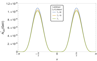
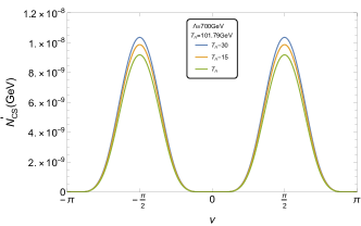
Figure 11: The $N_{CS}^{\prime}$ as function of $\nu$ at different temperature. These figures plot the value of $N_{CS}^{\prime}$ with $\Lambda=600$ GeV(Left), and $700$ GeV(Right) at different temperatures. The renormalization scale is set to $4\pi e^{-\gamma_{E}}T$.

The Fig. 11 shows the Chern-Simons number $N_{CS}^{\prime}$ as a function of $\nu$ at different temperatures. There is a periodic structure of $N_{CS}^{\prime}$ since the $N_{CS}^{\prime}$ is proportion to $\sin^{2}\nu$. The $N_{CS}^{\prime}$ decreases with increasing temperature, and this change is more pronounced at large $\Lambda$.

References

- Sakharov [1967] A. D. Sakharov, Violation of CP Invariance, C asymmetry, and baryon asymmetry of the universe, Pisma Zh. Eksp. Teor. Fiz. 5, 32 (1967).
- Grojean et al. [2005] C. Grojean, G. Servant, and J. D. Wells, First-order electroweak phase transition in the standard model with a low cutoff, Phys. Rev. D 71, 036001 (2005), arXiv:hep-ph/0407019 .
- Grojean and Servant [2007] C. Grojean and G. Servant, Gravitational Waves from Phase Transitions at the Electroweak Scale and Beyond, Phys. Rev. D 75, 043507 (2007), arXiv:hep-ph/0607107 .
- Zhou et al. [2020] R. Zhou, L. Bian, and H.-K. Guo, Connecting the electroweak sphaleron with gravitational waves, Phys. Rev. D 101, 091903 (2020), arXiv:1910.00234 [hep-ph] .
- Bian et al. [2020] L. Bian, H.-K. Guo, Y. Wu, and R. Zhou, Gravitational wave and collider searches for electroweak symmetry breaking patterns, Phys. Rev. D 101, 035011 (2020), arXiv:1906.11664 [hep-ph] .
- Alves et al. [2019] A. Alves, T. Ghosh, H.-K. Guo, K. Sinha, and D. Vagie, Collider and Gravitational Wave Complementarity in Exploring the Singlet Extension of the Standard Model, JHEP 04, 052, arXiv:1812.09333 [hep-ph] .
- Jiang et al. [2016] M. Jiang, L. Bian, W. Huang, and J. Shu, Impact of a complex singlet: Electroweak baryogenesis and dark matter, Phys. Rev. D 93, 065032 (2016), arXiv:1502.07574 [hep-ph] .
- Cline et al. [2011] J. M. Cline, K. Kainulainen, and M. Trott, Electroweak Baryogenesis in Two Higgs Doublet Models and B meson anomalies, JHEP 11, 089, arXiv:1107.3559 [hep-ph] .
- Dorsch et al. [2013] G. C. Dorsch, S. J. Huber, and J. M. No, A strong electroweak phase transition in the 2HDM after LHC8, JHEP 10, 029, arXiv:1305.6610 [hep-ph] .
- Dorsch et al. [2014] G. C. Dorsch, S. J. Huber, K. Mimasu, and J. M. No, Echoes of the Electroweak Phase Transition: Discovering a second Higgs doublet through , Phys. Rev. Lett. 113, 211802 (2014), arXiv:1405.5537 [hep-ph] .
- Bernon et al. [2018] J. Bernon, L. Bian, and Y. Jiang, A new insight into the phase transition in the early Universe with two Higgs doublets, JHEP 05, 151, arXiv:1712.08430 [hep-ph] .
- Andersen et al. [2018] J. O. Andersen, T. Gorda, A. Helset, L. Niemi, T. V. I. Tenkanen, A. Tranberg, A. Vuorinen, and D. J. Weir, Nonperturbative Analysis of the Electroweak Phase Transition in the Two Higgs Doublet Model, Phys. Rev. Lett. 121, 191802 (2018), arXiv:1711.09849 [hep-ph] .
- Kainulainen et al. [2019] K. Kainulainen, V. Keus, L. Niemi, K. Rummukainen, T. V. I. Tenkanen, and V. Vaskonen, On the validity of perturbative studies of the electroweak phase transition in the Two Higgs Doublet model, JHEP 06, 075, arXiv:1904.01329 [hep-ph] .
- Zhou et al. [2019] R. Zhou, W. Cheng, X. Deng, L. Bian, and Y. Wu, Electroweak phase transition and Higgs phenomenology in the Georgi-Machacek model, JHEP 01, 216, arXiv:1812.06217 [hep-ph] .
- Bian et al. [2018] L. Bian, H.-K. Guo, and J. Shu, Gravitational Waves, baryon asymmetry of the universe and electric dipole moment in the CP-violating NMSSM, Chin. Phys. C 42, 093106 (2018), [Erratum: Chin.Phys.C 43, 129101 (2019)], arXiv:1704.02488 [hep-ph] .
- Huber et al. [2016] S. J. Huber, T. Konstandin, G. Nardini, and I. Rues, Detectable Gravitational Waves from Very Strong Phase Transitions in the General NMSSM, JCAP 03, 036, arXiv:1512.06357 [hep-ph] .
- Mazumdar and White [2019] A. Mazumdar and G. White, Review of cosmic phase transitions: their significance and experimental signatures, Rept. Prog. Phys. 82, 076901 (2019), arXiv:1811.01948 [hep-ph] .
- Caprini et al. [2016] C. Caprini et al., Science with the space-based interferometer eLISA. II: Gravitational waves from cosmological phase transitions, JCAP 04, 001, arXiv:1512.06239 [astro-ph.CO] .
- Caprini et al. [2020] C. Caprini et al., Detecting gravitational waves from cosmological phase transitions with LISA: an update, JCAP 03, 024, arXiv:1910.13125 [astro-ph.CO] .
- Durrer and Neronov [2013] R. Durrer and A. Neronov, Cosmological Magnetic Fields: Their Generation, Evolution and Observation, Astron. Astrophys. Rev. 21, 62 (2013), arXiv:1303.7121 [astro-ph.CO] .
- Subramanian [2016] K. Subramanian, The origin, evolution and signatures of primordial magnetic fields, Rept. Prog. Phys. 79, 076901 (2016), arXiv:1504.02311 [astro-ph.CO] .
- Xu and Han [2022] J. Xu and J. L. Han, Evidence for Strong Intracluster Magnetic Fields in the Early Universe, Astrophys. J. 926, 65 (2022), arXiv:2112.01763 [astro-ph.CO] .
- Han et al. [2003] J.-L. Han, R. N. Manchester, G. J. Qiao, and A. G. Lyne, The Large - scale galactic magnetic field structure and pulsar rotation measures, ASP Conf. Ser. 302, 253 (2003), arXiv:astro-ph/0211197 .
- Joyce and Shaposhnikov [1997] M. Joyce and M. E. Shaposhnikov, Primordial magnetic fields, right-handed electrons, and the Abelian anomaly, Phys. Rev. Lett. 79, 1193 (1997), arXiv:astro-ph/9703005 .
- Campbell et al. [1992] B. A. Campbell, S. Davidson, J. R. Ellis, and K. A. Olive, On the baryon, lepton flavor and right-handed electron asymmetries of the universe, Phys. Lett. B 297, 118 (1992), arXiv:hep-ph/9302221 .
- Giovannini and Shaposhnikov [1998a] M. Giovannini and M. E. Shaposhnikov, Primordial hypermagnetic fields and triangle anomaly, Phys. Rev. D 57, 2186 (1998a), arXiv:hep-ph/9710234 .
- Giovannini and Shaposhnikov [1998b] M. Giovannini and M. E. Shaposhnikov, Primordial magnetic fields, anomalous isocurvature fluctuations and big bang nucleosynthesis, Phys. Rev. Lett. 80, 22 (1998b), arXiv:hep-ph/9708303 .
- Giovannini [2000a] M. Giovannini, Hypermagnetic knots, Chern-Simons waves and the baryon asymmetry, Phys. Rev. D 61, 063502 (2000a), arXiv:hep-ph/9906241 .
- Giovannini [2000b] M. Giovannini, Primordial hypermagnetic knots, Phys. Rev. D 61, 063004 (2000b), arXiv:hep-ph/9905358 .
- Boyarsky et al. [2012a] A. Boyarsky, J. Frohlich, and O. Ruchayskiy, Self-consistent evolution of magnetic fields and chiral asymmetry in the early Universe, Phys. Rev. Lett. 108, 031301 (2012a), arXiv:1109.3350 [astro-ph.CO] .
- Boyarsky et al. [2012b] A. Boyarsky, O. Ruchayskiy, and M. Shaposhnikov, Long-range magnetic fields in the ground state of the Standard Model plasma, Phys. Rev. Lett. 109, 111602 (2012b), arXiv:1204.3604 [hep-ph] .
- Rostam Zadeh and Gousheh [2016] S. Rostam Zadeh and S. S. Gousheh, Contributions to the UY(1) Chern-Simons term and the evolution of fermionic asymmetries and hypermagnetic fields, Phys. Rev. D 94, 056013 (2016), arXiv:1512.01942 [hep-ph] .
- Boyarsky et al. [2015] A. Boyarsky, J. Frohlich, and O. Ruchayskiy, Magnetohydrodynamics of Chiral Relativistic Fluids, Phys. Rev. D 92, 043004 (2015), arXiv:1504.04854 [hep-ph] .
- Semikoz and Sokoloff [2004] V. B. Semikoz and D. D. Sokoloff, Large - scale magnetic field generation by alpha-effect driven by collective neutrino - plasma interaction, Phys. Rev. Lett. 92, 131301 (2004), arXiv:astro-ph/0312567 .
- Semikoz and Sokoloff [2005a] V. B. Semikoz and D. D. Sokoloff, Magnetic helicity and cosmological magnetic field, Astron. Astrophys. 433, L53 (2005a), arXiv:astro-ph/0411496 .
- Semikoz and Sokoloff [2005b] V. B. Semikoz and D. D. Sokoloff, Large-scale cosmological magnetic fields and magnetic helicity, Int. J. Mod. Phys. D 14, 1839 (2005b).
- Semikoz et al. [2009] V. B. Semikoz, D. D. Sokoloff, and J. W. F. Valle, Is the baryon asymmetry of the Universe related to galactic magnetic fields?, Phys. Rev. D 80, 083510 (2009), arXiv:0905.3365 [hep-ph] .
- Akhmet’ev et al. [2010] P. M. Akhmet’ev, V. B. Semikoz, and D. D. Sokoloff, Flow of hypermagnetic helicity in the embryo of a new phase in the electroweak phase transition, Pisma Zh. Eksp. Teor. Fiz. 91, 233 (2010), arXiv:1002.4969 [astro-ph.CO] .
- Dvornikov and Semikoz [2012] M. Dvornikov and V. B. Semikoz, Leptogenesis via hypermagnetic fields and baryon asymmetry, JCAP 02, 040, [Erratum: JCAP 08, E01 (2012)], arXiv:1111.6876 [hep-ph] .
- Semikoz et al. [2012] V. B. Semikoz, D. D. Sokoloff, and J. W. F. Valle, Lepton asymmetries and primordial hypermagnetic helicity evolution, JCAP 06, 008, arXiv:1205.3607 [astro-ph.CO] .
- Dvornikov and Semikoz [2013] M. Dvornikov and V. B. Semikoz, Lepton asymmetry growth in the symmetric phase of an electroweak plasma with hypermagnetic fields versus its washing out by sphalerons, Phys. Rev. D 87, 025023 (2013), arXiv:1212.1416 [astro-ph.CO] .
- Semikoz et al. [2013] V. B. Semikoz, A. Y. Smirnov, and D. D. Sokoloff, Hypermagnetic helicity evolution in early universe: leptogenesis and hypermagnetic diffusion, JCAP 10, 014, arXiv:1309.4302 [astro-ph.CO] .
- Semikoz and Smirnov [2015] V. B. Semikoz and A. Y. Smirnov, Leptogenesis in the Symmetric Phase of the Early Universe: Baryon Asymmetry and Hypermagnetic Helicity Evolution, J. Exp. Theor. Phys. 120, 217 (2015), arXiv:1503.06758 [hep-ph] .
- Semikoz et al. [2016] V. B. Semikoz, A. Y. Smirnov, and D. D. Sokoloff, Generation of hypermagnetic helicity and leptogenesis in the early Universe, Phys. Rev. D 93, 103003 (2016), arXiv:1604.02273 [hep-ph] .
- Pavlović et al. [2016] P. Pavlović, N. Leite, and G. Sigl, Modified Magnetohydrodynamics Around the Electroweak Transition, JCAP 06, 044, arXiv:1602.08419 [astro-ph.CO] .
- Fujita and Kamada [2016] T. Fujita and K. Kamada, Large-scale magnetic fields can explain the baryon asymmetry of the Universe, Phys. Rev. D 93, 083520 (2016), arXiv:1602.02109 [hep-ph] .
- Kamada and Long [2016a] K. Kamada and A. J. Long, Baryogenesis from decaying magnetic helicity, Phys. Rev. D 94, 063501 (2016a), arXiv:1606.08891 [astro-ph.CO] .
- Anber and Sabancilar [2015] M. M. Anber and E. Sabancilar, Hypermagnetic Fields and Baryon Asymmetry from Pseudoscalar Inflation, Phys. Rev. D 92, 101501 (2015), arXiv:1507.00744 [hep-th] .
- Kamada and Long [2016b] K. Kamada and A. J. Long, Evolution of the Baryon Asymmetry through the Electroweak Crossover in the Presence of a Helical Magnetic Field, Phys. Rev. D 94, 123509 (2016b), arXiv:1610.03074 [hep-ph] .
- Vachaspati [2001] T. Vachaspati, Estimate of the primordial magnetic field helicity, Phys. Rev. Lett. 87, 251302 (2001), arXiv:astro-ph/0101261 .
- Qin and Bian [2024] R. Qin and L. Bian, First-order electroweak phase transition at finite density, JHEP 08, 157, arXiv:2407.01981 [hep-ph] .
- Yang and Bian [2022] J. Yang and L. Bian, Magnetic field generation from bubble collisions during first-order phase transition, Phys. Rev. D 106, 023510 (2022), arXiv:2102.01398 [astro-ph.CO] .
- Baym and Heiselberg [1997] G. Baym and H. Heiselberg, The Electrical conductivity in the early universe, Phys. Rev. D 56, 5254 (1997), arXiv:astro-ph/9704214 .
- Cohen et al. [1993] A. G. Cohen, D. B. Kaplan, and A. E. Nelson, Progress in electroweak baryogenesis, Ann. Rev. Nucl. Part. Sci. 43, 27 (1993), arXiv:hep-ph/9302210 .
- Boyarsky et al. [2021] A. Boyarsky, V. Cheianov, O. Ruchayskiy, and O. Sobol, Evolution of the Primordial Axial Charge across Cosmic Times, Phys. Rev. Lett. 126, 021801 (2021), arXiv:2007.13691 [hep-ph] .
- Kahniashvili et al. [2013] T. Kahniashvili, A. G. Tevzadze, A. Brandenburg, and A. Neronov, Evolution of Primordial Magnetic Fields from Phase Transitions, Phys. Rev. D 87, 083007 (2013), arXiv:1212.0596 [astro-ph.CO] .
- Brandenburg et al. [2017] A. Brandenburg, T. Kahniashvili, S. Mandal, A. Roper Pol, A. G. Tevzadze, and T. Vachaspati, Evolution of hydromagnetic turbulence from the electroweak phase transition, Phys. Rev. D 96, 123528 (2017), arXiv:1711.03804 [astro-ph.CO] .
- Taylor et al. [2011] A. M. Taylor, I. Vovk, and A. Neronov, Extragalactic magnetic fields constraints from simultaneous GeV-TeV observations of blazars, Astron. Astrophys. 529, A144 (2011), arXiv:1101.0932 [astro-ph.HE] .
- Banerjee and Jedamzik [2004] R. Banerjee and K. Jedamzik, The Evolution of cosmic magnetic fields: From the very early universe, to recombination, to the present, Phys. Rev. D 70, 123003 (2004), arXiv:astro-ph/0410032 .
- Ackermann et al. [2018] M. Ackermann et al. (Fermi-LAT), The Search for Spatial Extension in High-latitude Sources Detected by the Large Area Telescope, Astrophys. J. Suppl. 237, 32 (2018), arXiv:1804.08035 [astro-ph.HE] .
- Stevens et al. [2012] T. Stevens, M. B. Johnson, L. S. Kisslinger, and E. M. Henley, Non-Abelian Higgs model of magnetic field generation during a cosmological first-order electroweak phase transition, Phys. Rev. D 85, 063003 (2012).
- Gynther [2003] A. Gynther, Electroweak phase diagram at finite lepton number density, Phys. Rev. D 68, 016001 (2003), arXiv:hep-ph/0303019 .
- Laine [2005] M. Laine, Real-time Chern-Simons term for hypermagnetic fields, JHEP 10, 056, arXiv:hep-ph/0508195 .
- Kuzmin et al. [1985] V. A. Kuzmin, V. A. Rubakov, and M. E. Shaposhnikov, On the Anomalous Electroweak Baryon Number Nonconservation in the Early Universe, Phys. Lett. B 155, 36 (1985).
- Cline et al. [1993] J. M. Cline, K. Kainulainen, and K. A. Olive, On the erasure and regeneration of the primordial baryon asymmetry by sphalerons, Phys. Rev. Lett. 71, 2372 (1993), arXiv:hep-ph/9304321 .
- Linde [1983] A. D. Linde, Decay of the False Vacuum at Finite Temperature, Nucl. Phys. B 216, 421 (1983), [Erratum: Nucl.Phys.B 223, 544 (1983)].
- Guada et al. [2020] V. Guada, M. Nemevšek, and M. Pintar, FindBounce: Package for multi-field bounce actions, Comput. Phys. Commun. 256, 107480 (2020), arXiv:2002.00881 [hep-ph] .
- Lewicki et al. [2022] M. Lewicki, M. Merchand, and M. Zych, Electroweak bubble wall expansion: gravitational waves and baryogenesis in Standard Model-like thermal plasma, JHEP 02, 017, arXiv:2111.02393 [astro-ph.CO] .
- Steinhardt [1982] P. J. Steinhardt, Relativistic Detonation Waves and Bubble Growth in False Vacuum Decay, Phys. Rev. D 25, 2074 (1982).