Transverse voltage in anisotropic hydrodynamic conductors

Abstract

Weak momentum dissipation in ultra-clean metals gives rise to novel non-Ohmic current flow, including ballistic and hydrodynamic regimes. Recently, hydrodynamic flow has attracted intense interest because it presents a valuable window into the electronic correlations and the longest lived collective modes of quantum materials. However, diagnosing viscous flow is difficult as the macroscopic observables of ballistic and hydrodynamic transport such as the average current distribution can be deceptively similar, even if their respective microscopics deviate notably. Based on kinetic Boltzmann theory, here we propose to address this issue via the transverse channel voltage at zero magnetic field, which can efficiently detect hydrodynamic flow in a number of materials. To this end, we show that the transverse voltage is sensitive to the interplay between anisotropic fermiology and boundary scattering, resulting in a non-trivial behavior in narrow channels along crystalline low-symmetry directions. We discuss several materials where the channel-size dependent stress of the quantum fluid leads to a characteristic sign change of the transverse voltage as a new hallmark of the cross-over from the ballistic to the hydrodynamic regime.

Introduction.— Hydrodynamic electron flow is a special transport regime which onsets when a rapid electron-electron scattering rate exceeds all other relaxation mechanisms. In recent years, its fundamental importance became apparent in understanding the longest lived collective modes of correlated electrons [1, 2, 3, 4]. For example, viscous (hydrodynamic) correlations can shed light on electronic collective behavior, on the interacting phase diagram, and reveal unusual characteristics in the electron dynamics [5, 6, 7]. Hydrodynamic electron flow has also been discussed in connection to THz electromagnetic radiation in transistors [8, 9, 10], ambipolar transports in semiconductors/semimetals [11, 12, 13] and fluid spintronics [14, 15, 16, 17]. The current conceptual frontiers of interacting Fermi liquids are found in understanding correlations on the nanoscale, either due to extreme scattering rates in strongly correlated electron systems such as high-T_c superconductors, or due to nanoconfinement in heterostructures such as the nanoscopic channel sizes of current transistors. Advancing these goals necessitates experimental approaches sensing momentum diffusion in confined conductors. The last few years saw tremendous experimental progress in the imaging [18, 19, 20, 21, 22, 23] and characterization [24, 25, 26, 4] of the crossover regime between hydrodynamic and ballistic flow. At the same time, these efforts have also revealed that the actual flow profile of a quantum fluid in thin channels is rather ambiguous with respect to the dominant relaxation mechanism [27]. While it is possible to alleviate this issue by choosing other geometries [28, 29, 21, 30] or measure at finite magnetic field [31, 32], identifying more easily accessible characteristics which are sensitive to the ballistic-hydrodynamic crossover is highly sought after. The key point of this paper is to establish the transverse channel voltage in anisotropic conductors as such an accessible characteristic.

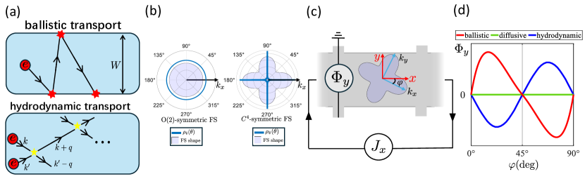
Figure 1: (a) Ballistic and hydrodynamic transport regimes. The red star represents scattering events with the boundary, while a yellow one represents the MC two-body scattering between electrons. (b) Representative Fermi surfaces with continuous rotational symmetry and with anisotropy. $\rho_{\hat{v}}$ denotes the distribution of Fermi velocity directions, shown in a polar histogram. (c) A four point geometry for measurements of transverse voltages with misalignment angle $\varphi$ between the crystal principle axis and the channel direction. (d) Schematics of the transverse voltage as a function of misalignment angle in different regimes for a Fermi surface with $C_{4}$ symmetry.

Electron transport in mesoscopic conductors is characterized by three characteristic length scales  [33]: The system size $W$, the momentum-relaxing (MR) mean-free path $\ell_{\mathrm{mr}}$, and the momentum-conserving (MC) mean-free path $\ell_{\mathrm{mc}}$. In very clean systems it holds that $W\ll\ell_{\mathrm{mr}}$ and Ohm’s law no longer describes the local relationship between electric field and current. The system therefore becomes ballistic if $W\ll\ell_{\mathrm{mr}}\ll\ell_{\mathrm{mc}}$ or hydrodynamic if $\ell_{\mathrm{mc}}\ll W\ll\ell_{\mathrm{mr}}$ (Fig. 1a).

In previous studies, the crossover regime (Gurzhi regime) when all three length scales are comparable ($W\approx\ell_{\mathrm{mr}}\approx\ell_{\mathrm{mc}}$) has been studied theoretically by a Boltzmann kinetic approach with a Callaway two-rate ansatz for isotropic Fermi surfaces  [34, 33, 35, 32]. The implicit assumption for this starting point is that the simplified isotropic description ought to capture the qualitative features of the ballistic-hydrodynamic crossover. However, this is far from obvious: From the point of view of theory, the limited attention to anisotropic effects means that essential parts of the kinetic approach have never been developed to take into account viscous correlations in an anisotropic system. Experimentally, it is important to investigate the sensitivity of observables such as flow profiles against inevitable misalignments between the channel and the crystal axes. Since several candidate materials with hydrodynamic electronic transport are in fact metals with anisotropic Fermi surfaces [24, 36, 19], it is critical to investigate the effect of symmetry breaking through the channel walls on the often subtle signatures of hydrodynamic flow. One might even ask if the Fermi surface shape can provide valuable insight for the ballistic-hydrodynamic crossover of a quantum fluid. Theoretical efforts to explore anisotropic effects in hydrodynamic conductors include broadband microwave spectroscopy [37, 38], a non-monotonic temperature and width dependence of the channel conductance [39], and viscous flow profiles on a Corbino disk [40].

Here, we address this question by examining the transverse voltage in the absence of magnetic field. Our main focus is anisotropic systems (Fig. 1b) lacking mirror symmetry due to a directional mismatch between the high symmetry axis of the Fermi surface and the geometric axis of the channel (Fig. 1c). To describe these systems, we generalise the Callaway ansatz to any two-dimensional anisotropic system, finding that a transverse voltage emerges at zero magnetic field which is strongly sensitive to the microscopic scattering mechanism. In particular, we show that the sign of the transverse voltage depends both on the Fermi surface shape and also the MC scattering rate. Under certain conditions, a sign reversal can indicate that the system crosses over from ballistic to hydrodynamic flow (Fig. 1d), which can serve as a sensitive observable for the crossover. We explain these subtle changes as the result of a competition of the transverse stress induced by the boundaries against the stress resulting from the bulk MR scattering. Using the sign to identify the onset of hydrodynamic regimes offers several advantages. Firstly, it only requires a non-spatially resolved transport measurement of a single device. Secondly, the sign change of the transverse voltage is uncommon outside the hydrodynamic context, as in other regimes, it typically only relates to the carrier type of the material. Although the sign change strongly suggests a crossover, it does not mark a precise boundary between the ballistic and hydrodynamic regimes, as this is not a phase transition. In short, we suggest the signature of the transverse voltage as a relatively straightforward experimental observable for detecting non-local hydrodynamic transport. Additionally, our work establishes a general framework to treat anisotropic ballistic and hydrodynamic transport in systems with $C_{4}$ rotational symmetry or higher.

Collisional invariants for anisotropic Fermi surfaces.— We aim to describe the ballistic-hydrodynamic crossover using semiclassical kinetics. The starting point is the Boltzmann transport equation (BTE) for the distribution function $f$, given by $(\partial_{t}+\mathbf{v}_{\mathbf{k}}\cdot\nabla_{\mathbf{r}}+\mathbf{F}\cdot\nabla_{\mathbf{k}})f(\mathbf{r},\mathbf{p},t)=C[f(\mathbf{r},\mathbf{p},t)]$, where $C$ is the collision integral and $\mathbf{F}$ is the perturbation. It is common to parametrize the deviation from the equilibrium state by writing $f(\mathbf{r},\mathbf{p},t)-f^{0}(\varepsilon_{\mathbf{p}})=-E_{F}\partial_{\varepsilon}f^{0}(\epsilon)h(\mathbf{r},\mathbf{p},t)$, where $E_{F}$ is the Fermi energy and $h$ is dimensionless non-equilibrium distribution function. In the following, we consider the low temperature limit where $\partial_{\varepsilon}f^{0}(\varepsilon)\approx-\delta(\epsilon-E_{F})$. This is a good assumption for materials with a large carrier density since the actual temperature is significantly lower than the Fermi temperature. In experiment, variations in temperature usually have a greater impact on the scattering rate than on the thermal broadening of the distribution function. For the sake of simplicity, we consider a Fermi surface for which a bijection between angular variable $\theta$ and Fermi wave vector $\mathbf{p}_{F}$ exits. This allows to integrate out the radial momentum dependence of $\mathbf{p}$, leaving only an angular momentum variable $\theta$. In more general scenarios, the Fermi surface arclength should be employed instead.

We begin by defining a bra-ket notation for the BTE [41, 39, 37]. Let $g(\mathbf{r},\theta,t)$ be a state function on the Fermi surface. Then the corresponding ket and inner product in two-dimension are defined by

$$\ket{g(\mathbf{r},t)} = \int{d\theta}\sqrt{\frac{p_{F}^{2}(\theta)E_{F}}{{(2\pi\hbar)^{2}|\mathbf{v}_{F}(\theta)\cdot\mathbf{p}_{F}(\theta)|}}}g(\mathbf{r},\theta,t)\ket{\theta}$$ (1)

where $\bra{{\theta}}\ket{{\theta^{\prime}}}=\delta(\theta-\theta^{\prime})$. With this definition , $\expectationvalue{g(\mathbf{r},t)}=\bra{h(\mathbf{r},t)}\ket{g(\mathbf{r},t)}$.

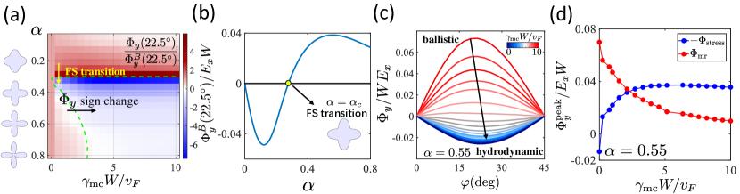
Figure 2: (a)Transverse voltage at $22.5^{\circ}$ normalized by the ballistic value, shown as a function of both Fermi surface anisotropy $\alpha$ and dimensionless MC rate. Green dotted line: interpolated boundary line when transverse voltage is vanishing. Yellow arrow: Fermi surface transition happens at $\alpha\approx 0.3$, corresponding to a sign-change of ballistic transverse voltage, black arrow: a line-cut for a fixed Fermi surface, where transverse voltage changes sign with increase MC rate. (b) Ballistic transverse voltage as a function of $\alpha$. Yellow dot: non-trivial zero of the ballistic transverse voltage signifying the Fermi surface transition. (c) Transverse volatge as a function of misalignment angle $\varphi$, parameters are taken as indicated by the black line cut in (a). From ballistic to hydrodynamic region, the transverse voltage flips its sign. (d) Decomposition of the transverse volatge. As MC rate increases, MR contribution is decreasing to zero and the stress component is dominant.

For convenience, we abbreviate the metric in phase space as $A(\theta)={{p_{F}^{2}(\theta)E_{F}}/{{(2\pi\hbar)^{2}|\mathbf{v}_{F}(\theta)\cdot\mathbf{p}_{F}(\theta)|}}}$ and define the following modes with unit length: A particle mode called $\ket{c}\propto\int d\theta\sqrt{A(\theta)}\ket{\theta}$, corresponding to the particle number, and a momentum mode called $\ket{p_{\mu}}\propto\int d\theta\sqrt{A(\theta)}p_{\mu}(\theta)\ket{\theta}$, which will be relevant for contractions which preserve momentum  [41, 39, 37, 24, 33, 42].

To proceed, we need to make some assumptions about the collision integral $C$. Here, we take the Callaway two-rate ansatz [34] to construct phenomenological collision terms. The idea is to restrict $C$ to an universal subset of eigenmodes which are longest lived. For electron flow in a channel, these long-lived modes derive from particle number which is conserved exactly and momentum, which relaxes with a small scattering rate $\gamma_{\mathrm{mr}}$. Assuming that all other excitations relax at least as fast as these quasi-conserved quantities with rate $\gamma=\gamma_{\mathrm{mc}}+\gamma_{\mathrm{mr}}$ [39, 37], one obtains two collisional integrals,

$$C_{\mathrm{mr}} = -\gamma_{\mathrm{mr}}(\mathbbm{1}-\ket{c}\bra{c}),$$

$$C_{\mathrm{mc}} = -\gamma_{\mathrm{mc}}\left(\mathbbm{1}-\ket{c}\bra{c}-\sum_{\mu}\ket{p_{\mu}}\bra{p_{\mu}}\right).$$ (2)

Importantly, as long as $W\ll v_{F}/\gamma_{\mathrm{mr}}$, this construction guarantees both particle number and (approximate) momentum conservation since $\bra{c}C_{\mathrm{mr/mc}}\ket{h}=0$ and $\bra{p_{\mu}}C_{\mathrm{mc}}\ket{h}=0$.

Let us consider the transverse transport in a long narrow channel geometry (Fig. 1) at zero magnetic field and zero temperature. This geometry is assumed to be translationally invariant in the longitudinal direction (denoted $x$), thus the the distribution function only has a spatial dependence in $y$ direction. As a function of the remaining two parameters $(y,\theta)$,

the Boltzmann equation becomes,

$$D[h]=(C_{\mathrm{mr}}+C_{\mathrm{mc}})\ket{h},$$ (3)

where the drift terms are

$$D[h] = \partial_{y}\ket{v_{y}h}-E_{x}\ket{v_{x}}-E_{y}\ket{v_{y}}.$$ (4)

Here, $E_{x},E_{y}$ are electric fields normalized by the Fermi energy, having the same unit as a wave vector. We assume a fixed longitudinal electric field $E_{x}$ and view $E_{y}(y)$ as a response to the input field $E_{x}$.

Rearranging terms, one obtains

$$C_{0}\ket{h} =\sum_{\mu}E_{\mu}\ket{v_{\mu}}$$

$$+\bigg{[}\gamma\ket{c}\bra{c}+\gamma_{\mathrm{mc}}\sum_{\nu}\ket{p_{\nu}}\bra{p_{\nu}}\bigg{]}\ket{h},$$ (5)

where $C_{0}\ket{h}=\partial_{y}\ket{v_{y}h}+\gamma\ket{h}$. A proper diffusive boundary condition is imposed as $h^{\pm}(\mp W/2,\theta)=0$ and $J_{y}(y)\equiv\bra{v_{y}}\ket{h}=0.$ Here, $h^{\pm}(y,\theta)$ are $h(y,\theta)$ restricted to the the domain $\Theta^{\pm}=\{\theta|\mathrm{sign}[v_{y}(\theta)]=\pm 1\}$ respectively.

In this form, we can solve the BTE self-consistently and obtain the transverse electric field as $E_{y}(y)=\bra{p_{y}}\ket{v_{y}}^{-1}(\bra{p_{y}}C_{0}\ket{h}-\gamma_{\mathrm{mc}}\sum_{\mu}\bra{h}\ket{p_{\mu}}\bra{p_{\mu}}\ket{v_{y}})$. The transverse voltage is the integral $\Phi_{y}=\int dy\,E_{y}(y)$. We can clearly identify two different components in $\Phi_{y}$, which read explicitly $\Phi_{y}=\Phi_{y}^{\mathrm{stress}}+\Phi_{y}^{\mathrm{mr}}$, where

$$\Phi_{y}^{\mathrm{stress}} =\bra{p_{y}}\ket{v_{y}}^{-1}\bra{p_{y}}\ket{v_{y}h}\bigg{|}^{W/2}_{-W/2}$$

$$\Phi_{y}^{\mathrm{mr}} =\bra{p_{y}}\ket{v_{y}}^{-1}\gamma_{\mathrm{mr}}\int_{-W/2}^{W/2}dy\bra{p_{y}}\ket{h}$$ (6)

Here, $\Phi_{y}^{\mathrm{stress}}$ is related to the $yy$ component of the stress tensor $\Pi_{\mu\nu}\equiv\bra{p_{\mu}}\ket{v_{\nu}h}$ of the quantum fluid, whereas $\Phi_{y}^{\mathrm{mr}}$ is proportional to the MR rate $\gamma_{\mathrm{mr}}$.

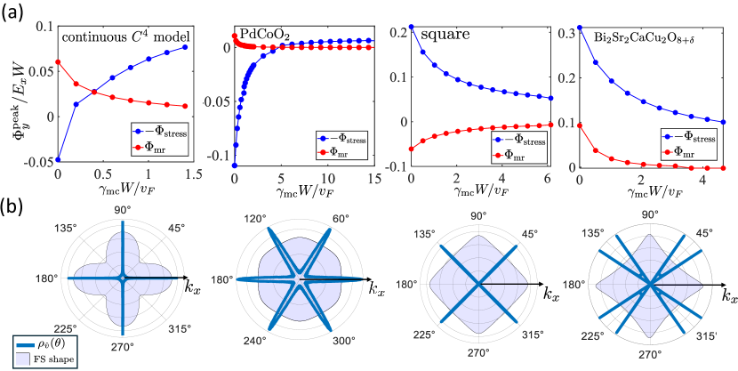
Figure 3: (a) Decomposition of the transverse voltage of different models. Left to right: $C_{4}$ model with a energy dispersion $\varepsilon(k)$ with $\gamma_{\mathrm{mr}}W/v_{F}=0.1$ [42], TB model for $\mathrm{PdCoO_{2}}$ [43] with $\gamma_{\mathrm{mr}}W/v_{F}=0.08$, TB square model with $\gamma_{\mathrm{mr}}W/v_{F}=0.49$ [42],TB model for over-doped cuprate $\mathrm{Bi2212}$ [44] with $\gamma_{\mathrm{mr}}W/v_{F}=0.49$. (b) Fermi velocity direction distribution plotted as a polar histogram plot.

Ballistic-hydrodynamic crossover.— In order to demonstrate the anisotropy effect of Fermi surface in a tractable manner, we use the following parameterization for the Fermi wave vector $k_{F}$ for a $C_{n}$ Fermi surface $k_{F}(\theta;\alpha,\varphi)=k_{F}^{0}\left\{1+\alpha\cos[n(\theta-\varphi)]\right\}$, where $\theta$ is the angle between $\mathbf{k}_{F}$ and the crystal $k_{x}$-axis, $\varphi$ is the angle between the crystal and channel axes as shown in Fig.2a. $\alpha$ is the controlling parameter for the Fermi surface shape. With varying $\alpha$, the Fermi surface goes from circular to cross-shaped, and finally flower-shaped, as shown in Fig.2a for $n=4$.

We mainly focus on non-Ohmic region, so we fix the MR rate $\gamma_{\mathrm{mr}}$ within the limit $\gamma_{\mathrm{mr}}W/v_{F}\lesssim 1$ and change the MC rate $\gamma_{\mathrm{mc}}$ to investigate the ballistic-hydrodynamic crossover. The transverse voltage at the misalignment angle $\varphi=22.5^{\circ}$ which marks the maximal transverse voltage in the ballistic case as a function of both Fermi surface shape and MC scattering rate is studied in Fig.2(a). In order to show the sign change of the transverse voltage, it is best to look at the normalized quantity $\Phi_{y}/\Phi_{B}$ where $\Phi_{B}$ is the ballistic voltage ($\gamma_{\mathrm{mc}}=0$). We observe that for a fixed small $\alpha<\alpha_{c}$, the transverse voltage remains of the same sign irrespective of the value of $\gamma_{\mathrm{mc}}$. At the critical value $\alpha_{c}\approx 0.3$, the increasingly anisotropic Fermi surface leads to a sign change of the ballistic voltage (yellow arrow). We should emphasize that the sign reverses when changing the Fermi surface shape is not due to the hydrodynamic nature, it is a direct consequence of the Fermi velocity distribution of different Fermi surfaces. In the supplemental material [42], we show that this latter sign change is determined by the quantity $\expectationvalue{v_{x}\mathrm{sign}(v_{y})}$. The physical picture is that for a given driven electric field $E_{x}$, the response to it is proportional to $v_{x}$, and $\text{sign}(v_{y})$ indicates the electrons moving to the top or bottom in the transverse direction of the channel.

More interestingly, for a fixed large $\alpha>\alpha_{c}$, with increasing MC scattering rate $\gamma_{\mathrm{mc}}$, the voltage exhibits an additional sign change between the ballistic region and the hydrodynamic region (cf. green dotted line in Fig. 2a). This latter sign change persists for basically all misalignment angles, as is shown in Fig. 2c. We can conclude that during the ballistic-hydrodynamic crossover, some anisotropic Fermi surfaces will cause the modulus of the transverse voltage to first decrease, cross zero smoothly and then increase with opposite sign. We further observe that $\Phi_{y}(\varphi)$ can have a quite asymmetric shape, which changes noticeably as a function of $\gamma_{\mathrm{mc}}$. As mentioned above Eq. (6), we want to understand the underlying mechanism for the transverse voltage by decomposing the voltage as an internal stress contribution and MR contribution. The two contributions to the stress are shown in Fig. 2d for the anisotropy parameter $\alpha=0.55$. $\Phi_{y}$ here is taken as the peak voltage in the whole range of $\varphi$ rotation at a fixed $\gamma_{\mathrm{mr}}$ and varying with $\gamma_{\mathrm{mc}}$. In essence, in the hydrodynamic regime such that $\gamma_{\mathrm{mc}}W/v_{F}\gg 1$, the MR component is vanishing so that the the internal stress of the quantum fluid becomes the dominant contribution to the transverse voltage. Conversely, the dissipative stress dominates at small $\gamma_{\mathrm{mc}}$, therefore there exists a critical $\gamma^{c}_{\mathrm{mc}}$ where the two contributions cancel and the sign of transverse voltage $\Phi_{y}$ reverses.

Material examples.— Here we present some instructive examples of anisotropic Fermi surfaces which additionally contain anisotropic Fermi velocities. We find that both a continuum model and tight-binding(TB) examples can exhibit a behavior very similar to the one discussed for the simplified scenario, thus confirming the robustness of our diagnosis. Namely, we focus on the ultra clean material $\mathrm{PdCoO_{2}}$ [24], and the overdoped strongly correlated cuprate $\mathrm{Bi_{2}Sr_{2}CaCu_{2}O_{8+\delta}(Bi2212)}$ [36], as in both non-Ohmic transport has been observed. For comparison, we also include a square lattice with nearest-neighbor hopping. The model details can be found in the supplemental material [42], the results of these calculations are shown in Fig. 3. Not surprisingly, in all cases the MR component is diminishing when approaching the hydrodynamic limit. Thus in the hydrodynamic region, the only contribution to transverse voltage is the $yy$ component of the stress tensor $\Pi_{\mu\nu}$. For the anisotropic $C_{4}$ model [42], our calculation reveals a sign change of the transverse voltage with increasing MC scattering rate, serving as a direct indicator of hydrodynamic transport. The location of this crossover, however, depends on the Fermi surface shape, the channel width, and the el-el scattering rate. For the Fermi surfaces of the square and Bi2212, for example, such a sign change would occur at extreme scattering rates inaccessible to our numerical implementation. Thus in a real material, these parameters may render the sign change inaccessible for realistic channel sizes.

This diagnostic methodology can be extended to treat those situations, thus greatly expanding its range of applicability. The transverse voltage results from a competition between $\Phi_{y}^{\mathrm{stress}}$ and $\Phi_{y}^{\mathrm{mr}}$, which in general scale differently with the channel misalignment angle $\varphi$ (see asymmetry evolution in Fig. 2c). Hence the transverse voltage difference between two channels symmetrically misaligned by an angle $\pm\delta\varphi$ to mutually adjacent mirror planes is a sensitive probe of emergent hydrodynamics (Fig 4). Its asymmetry is actually most pronounced in the weakly hydrodynamic sector of small $\gamma_{\mathrm{mc}}W/v_{F}$ and a channel width dependence allows a straightforward estimation of $\gamma_{\mathrm{mc}}$ through a transport experiment. The required simple geometry of two canted bars is sketched in Fig. 4a. Varying the channel width by a factor of 10 is straightforward lithographically, which will provide enough range to extract $\gamma_{\mathrm{mc}}$ even when the sign change itself cannot be accessed.

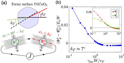
Figure 4: (a) Sketch for measurement of the difference of transverse voltage $\Phi_{y}^{a}-\Phi_{y}^{b}$ at misalignment angle $\varphi_{a}=\delta\varphi$ and $\varphi_{b}=30^{\circ}-\delta\varphi$ for $\mathrm{PdCoO_{2}}$. (b) Difference of transverse voltage as function of MC scattering rate. Inset: $\Phi_{y}^{a}$ and $\Phi_{y}^{b}$ as a function of MC scattering rate.

Conclusion.— By employing a Callaway two-rate ansatz, we have identified a non-vanishing transverse voltage for a wide range of low-symmetry transport configurations. We find that in a $C_{4}$-symmetric system, a sufficiently anisotropic Fermi surface can lead to a sign change in the transverse voltage as the electron fluid crosses over from ballistic to hydrodynamic transport. We therefore propose that measuring the transverse voltage at zero magnetic field can be a viable way to distinguish different types of non-Ohmic transport. The prescribed phenomenology offers an alternative probe for the experimental investigation of unconventional charge transport beyond the analysis of the current flow pattern. We reiterate that the measurement of transverse voltage seems particularly attractive because it does not require an external magnetic field or a local imaging of the current profile. We believe that the sign change is observable with current devices as a function of either gate voltage or temperature using the geometry depicted in Fig. 4. For example, in Ref. [24], the estimated range of $\gamma_{\mathrm{mr}}/\gamma_{\mathrm{mc}}$ is $0.05\sim 0.2$, based on fits of the conductivity to an isotropic model.

As a limitation of our results, let us mention that the simplifications to the collision integral used here cannot capture the intermediate tomographic transport regime  [45, 46, 47, 41]. Further refinements in the treatment of the full collision integral seem needed to treat these and similar effects in anisotropic materials. On the other hand, the methodology developed here can be extended straightforwardly to investigate hydrodynamic crossovers in three-dimensional systems.