Finite-Difference Approximations and Local Algorithms for the Poisson and Poisson–Boltzmann Electrostatics
Abstract
We study finite-difference approximations of both Poisson and Poisson–Boltzmann (PB) electrostatic energy functionals for periodic structures constrained by Gauss’ law and a class of local algorithms for minimizing the finite-difference discretization of such functionals. The variable of Poisson energy is the vector field of electric displacement and that for the PB energy consists of an electric displacement and ionic concentrations. The displacement is discretized at midpoints of edges of grid boxes while the concentrations are discretize at grid points. The local algorithm is an iteration over all the grid boxes that locally minimizes the energy on each grid box, keeping Gauss’ law satisfied. We prove that the energy functionals admit unique minimizers that are solutions to the corresponding Poisson’s and charge-conserved PB equation, respectively. Local equilibrium conditions are identified to characterize the finite-difference minimizers of the discretized energy functionals. These conditions are the curl free for the Poisson case and the discrete Boltzmann distributions for the PB case, respectively. Next, we obtain the uniform bound with respect to the grid size and -error estimates in maximum norm for the finite-difference minimizers. The local algorithms are detailed, and a new local algorithm with shift is proposed to treat the general case of a variable coefficient for the Poisson energy. We prove the convergence of all these local algorithms, using the characterization of the finite-difference minimizers. Finally, we present numerical tests to demonstrate the results of our analysis.
Key words and phrases: Gauss’ law, Poisson’s equation, the Poisson–Boltzmann equation, finite difference, error estimate, local algorithm, convergence, superconvergence.
AMS Subject Class: 49M20, 65N06, 65Z05.
1 Introduction
We consider the following variational problems of minimizing the non-dimensionalized Poisson [24, 23] and Poisson–Boltzmann (PB) [6, 12, 19, 2, 15, 52, 7, 27] electrostatic energy functionals constrained by Gauss’ law for periodic structures:
Here, is a cube, and are given -periodic functions representing the dielectric coefficient and a fixed charge density, respectively, and is an -periodic vector filed of electric displacement. For the PB case, and each is the local concentration of ions of th species, a total of species is assumed. For each , is the charge for an ion in species and is the total amount of concentration of such ions. All , , and are given constants. Here and below denotes the natural logarithm and if
To discretize the energy functionals and Gauss’ law, let us consider the three-dimensional case to be specific and cover with a finite-difference grid of size with the grid point corresponding to the spatial point . We approximate the displacement at half-grid points by and concentrations at grid points by for all The PB energy and the corresponding Gauss’ law at all the grid points are then discretized as
respectively, where and and are similarly defined, and is an approximation of . The mass conservation can be discretized similarly. The finite-difference discretization of the Poisson energy and that of the corresponding Gauss’ law are similar. Note that the discretization of displacement is a classical scheme for Maxwell’s equation for isotropic media [49] (cf. also [34, 30]). If the displacement is given by with an electrostatic potential , then the resulting scheme for is a commonly used, second-order central differencing scheme; cf. e.g., [36, 37].
We are interested in a class of local algorithms for electrostatics [33, 32, 4, 44, 35] that are based on the above formulation of the constrained energy minimization and the corresponding finite-difference discretization. The key idea of such algorithms is to keep Gauss’ law satisfied at each grid point while locally updating the discretized displacement or ionic concentrations one grid at a time, cycling through all the grid points iteratively. For instance, given a finite-difference displacement and a grid box , one updates locally the components of on the edges of the three faces of the grid box sharing the vertex to decrease the Poisson energy . Let us fix such a face to be the square with vertices , , , and To satisfy Gauss’ law at these vertices, we update
with a single parameter that can be readily computed to minimize the perturbed Poisson energy; cf. section 5.1 for more details. For the PB energy, the concentration and the displacement are locally updated at neighboring grids, e.g., and , and at the edge connecting them, respectively, by
with a single parameter that can be computed to minimize the perturbed PB energy. The special forms of these perturbations are determined by the mass conservation and Gauss’ law; cf. section 5.2 for more details.
Let us now briefly describe and discuss our main results.
(1) Existence, uniqueness, characterization, and bounds of minimizers. The constrained Poisson energy is uniquely minimized by , where is the unique solution to Poisson’s equation ; cf. Theorem 2.1.
Similarly, the unique minimizer of the constrained PB energy is given by and the Boltzmann distributions for all , where the electrostatic potential is the unique solution to the charge-conserved PB equation (CCPBE)
Moreover, a variational analysis of the CCPBE using a comparison argument [28] shows that is bounded function. This leads to the uniform positive bounds
(2) Characterization and uniform bounds of finite-difference minimizers. The unique minimizer of the discretized constrained Poisson energy is given by , where is the unique solution to the discretized Poisson’s equation. Moreover, is characterized by the local equilibrium condition and the global constraint
respectively, where is the discrete curl operator; cf. Theorem 3.1. These are analogous to the vanishing of curl and integral of gradient of a smooth and periodic function.
The unique finite-difference solution to the discretized CCPBE is uniformly bounded in the maximum norm with respect to the grid size This is proved using a similar comparison argument. The unique minimizer of the discretized constrained PB energy is then given by the discrete Boltzmann distributions and , where is the discrete gradient. These, together with the uniform positive bounds
with and constants independent of , characterize the discrete minimizer for the PB energy; cf. Theorem 3.2 and Theorem 3.3.
(3) Error estimates. We obtain the -error estimate for the finite-difference approximation of the Poisson energy minimizer
where for any continuous displacement and all , and denotes a generic constant independent of . This follows from the and stability of the inverse of the finite-difference operator for the Poisson equation [37, 36, 5]. By a simple averaging from , we obtain an approximation , a vector-valued grid function, and the superconvergence estimate
improving the existing -superconvergence estimate [30]; cf. Theorem 4.1 and Corollary 4.1.
For the PB case, we first prove the -error estimates for both the displacement and concentrations, relying on the uniform bounds on the discrete concentrations. Such estimates are then used to prove the -error estimate
cf. Theorem 4.2.
(4) A new local algorithm with shift for variable dielectric coefficient. Note that each local update in the local algorithm for relaxing the discrete Poisson energy does not change but will change if is not a constant. Therefore, the local algorithm for Poisson may not converge to the correct limit in this case, as the minimizer should satisfy the global constraint To resolve this issue, we propose a new local algorithm with shift: after a few cycles of local update of the displacement , we shift it by adding a constant vector to so that the shifted new displacement will satisfy the required global constraint; cf. section 5.1.
(5) Convergence of all the local algorithms. The proof relies crucially on the characterization of the finite-difference minimizers and of the discrete Poisson and PB energy functionals, respectively. If is the energy difference after the th local update, then as . Moreover, the amount of local change of the displacement or concentration in a local update is controlled by the energy difference. Therefore, the sequence of such local changes converge to a local equilibrium that satisfies the conditions characterizing the finite-difference minimizer; cf. Theorem 5.1, Theorem 5.2, and Theorem 5.3.
(6) Numerical tests. We present numerical tests to demonstrate the results of our analysis on the error estimates and the convergence of local algorithms; cf. section 6.
We remark that the PB equation [6, 12, 19, 2, 15, 52, 7, 27], with different kinds of boundary conditions, is a widely used continuum model of electrostatics for ionic solutions with many applications, particularly in molecular biology [22, 45, 9, 20, 21, 43, 16, 3, 53]. The periodic boundary conditions for Poisson’s and PB equations are commonly used for simulations of electrostatics not only for periodic charged structures such as ionic crystals but also in molecular dynamics simulations of charged molecules [41, 42, 10, 11, 17, 8, 14].
The local algorithms were initially proposed for Monte Carlo and molecular dynamics simulations of electrostatics and electromagnetics [33, 32, 44, 4, 35]. Such algorithms scale linearly with system sizes and are simple to implement. The Gauss’ law constrained energy minimization model for electrostatics that is the basis for the local algorithms has been extended to model ionic size effects with nonuniform ionic sizes [54, 29, 26]. Recently, the local algorithms have been incorporated into numerical methods for Poisson–Nernst–Planck equations [39, 38, 40]. The linear complexity and locality of the local algorithms make it appealing to combine them with the recently developed binary level-set method for large-scale molecular simulations using the variational implicit solvent model [51, 31, 50, 53].
The rest of this paper is organized as follows: In section 2, we first set up the variational problems of minimizing the Poisson and PB electrostatic energy functionals constrained by Gauss’ law. We then obtain the existence, uniqueness, and bounds in maximum norm of the energy minimizers through the corresponding electrostatic potentials that are the periodic solutions to Poisson’s equation and the CCPBE, respectively. In section 3, we define finite-difference approximations of the Poisson and PB energy functionals, identify sufficient and necessary conditions for the finite-difference energy minimizers, and obtain their uniform bounds in maximum norm independent of the grid size . In section 4, we prove the error estimates for the finite-difference energy minimizers. In section 5, we describe the local algorithms for minimizing the finite-difference functionals, and a new local algorithm with shift for minimizing the Poisson energy with a variable dielectric coefficient. We also prove the convergence of all these algorithms. In section 6, we report numerical tests to demonstrate the results of our analysis. Finally, in Appendix, we prove some properties of the finite-difference operators.
2 Energy Minimization
Let and with or . We denote by and () the spaces of -periodic continuous functions and -periodic -functions on , respectively. Let and We denote by and the spaces of all -periodic functions on such that their restrictions onto are in the Lebesgue space and the Sobolev space , respectively [18, 1, 13]. Note that any can be extended -periodically to after the values of on a set of zero Lebesgue measure are modified if necessary. As usual, two functions in or are the same if and only if they equal to each other almost everywhere with respect to the Lebesgue measure. We define
where for a Lebesgue measurable function defined on a Lebesgue measurable set of finite measure ,
| (2.1) |
We denote and . By Poincaré’s inequality, is a norm of , equivalent to the -norm. We further define
The divergence is understood in the weak sense. The space is a Hilbert space with the corresponding norm [46].
2.1 The Poisson energy
We consider the Poisson electrostatic energy with a given charge density . Denote
| (2.2) | ||||
| (2.3) |
By the periodic boundary condition and the divergence theorem, if and only if Clearly Let . Assume there exist such that
| (2.4) |
We define
| (2.5) | ||||
| (2.6) |
Theorem 2.1.
Let satisfy (2.4) and .
-
(1)
There exists a unique such that Moreover, is the unique weak solution in to Poisson’s equation defined by
(2.7) -
(2)
There exists a unique such that Moreover, the minimizer is characterized by and
(2.8) -
(3)
We have
2.2 The charge-conserved Poisson–Boltzmann equation
Let be an integer, nonzero real numbers, positive numbers, satisfy (2.4), and We shall assume the following:
| (2.9) |
Let us define by [25]
| (2.10) |
Lemma 2.1.
(1) for any and any constant
(2) The functional is strictly convex;
(3) There exist and such that for all
Proof.
(1) This follows from the charge neutrality (2.9).
(2) The integral part of the functional is strictly convex as is a norm on The convexity of the non-integral part of the functional follows from an application of Holder’s inequality and the fact that is an increasing function on
(3) This follows from Jensen’s inequality applied to and Poincaré’s inequality applied to ∎
By formal calculations, the Euler–Lagrange equation for the functional defined in (2.10) is the charge-conserved Poisson–Boltzmann equation (CCPBE)
| (2.11) |
Definition 2.1.
A function is a weak solution to the CCPBE (2.11) if for each and
| (2.12) |
Theorem 2.2.
Remark 2.1.
These results are generally known for the case that for some and for some other [25]. Here we include the case that all or all . Moreover, we present a proof with a key difference. We obtain the -bound of the minimizer by a comparison argument; cf. [28]. The bound allows us to apply the Lebesgue Dominated Convergence Theorem to show that the minimizer is a weak solution to the CCPBE. The comparison method used in obtaining the bound will also be used in section 3.3 to obtain a uniform bound for finite-difference approximations of the solution to CCPBE.
Proof of Theorem 2.2.
The existence of a minimizer follows from Lemma 2.1 and a standard argument by direct methods in the calculus of variations; cf. e.g., [25]. The uniqueness of a minimizer follows from the strict convexity of the functional
We now assume in addition that and prove that Let be the unique weak solution to Poisson’s equation with the periodic boundary condition, defined by
cf. Theorem 2.1. By the regularity theory, [18]. We define
| (2.13) |
Let and set ; cf. (2.1). We verify directly that
| (2.14) |
where If with , then
Thus, is the unique minimizer of and is finite since is.
We show that which implies We consider three cases.
Case 1: there exist such that and . Let and define
| (2.15) |
Clearly, and Since , we have . Therefore, it follows from (2.14), (2.15), and Jensen’s inequality applied to that
| (2.16) |
where
| (2.17) |
Note that for each . Since is finite, we also have for each . Denoting , we have by (2.15) and the fact that that
| (2.18) |
We can verify directly that is convex. Moreover, since and , and . Thus, since , and a.e. , if is large enough. Consequently, it follows from (2.2), (2.2), and an application of Jensen’s inequality that
Hence, , i.e., a.e. . Thus,
Case 2: all In this case, defined in (2.17) is convex and For any , we define now if and if and Clearly, and . Carrying out the same calculations as above with replacing , we get for large enough that
where is the same as in (2.2). Thus, a.e. Since and all , for each Since is the minimizer of defined in (2.13) over , we now have by direct calculations that
Since and is bounded above, for each . Thus, weakly. Consequently, weakly. Hence, and further
Case 3: all This is similar to Case 2.
Finally, since is the unique minimizer of we obtain by routine calculations the equation in (2.12) with By approximations, (2.12) is true. Thus, is a weak solution to the CCPBE with the periodic boundary condition. This also implies that in weak sense. The regularity theory then implies that and finally (2.11) holds true a.e. in
Assume are two weak solutions of the CCPBE. Denote
Each is a convex function. Thus,
Consequently, it follows from (2.12) with and that
Hence, in and the weak solution is unique. ∎
2.3 The Poisson–Boltzmann energy
Let satisfy (2.9). We consider now ionic concentrations and the electric displacements that satisfy the following:
| Nonnegativity: | (2.19) | ||||
| Mass conservation: | (2.20) | ||||
| Gauss’ law: | (2.21) |
We define
| (2.22) | ||||
| (2.23) |
Lemma 2.2.
Let Then, if and only if (2.9) holds true.
Proof.
Let satisfy (2.4). We define by
| (2.24) |
Theorem 2.3.
(1) Let be given by
| (2.25) | ||||
| (2.26) |
where is the unique weak solution to the CCPBE as given in Theorem 2.2. Then is the unique minimizer of
(2) Let . Then if and only if the following conditions are satisfied:
-
(i)
Positive bounds: There exist such that for a.e. and all
-
(ii)
Global equilibrium:
(2.27)
3 Finite-Difference Approximations
We shall focus on the dimension from now on. The case that the dimension is similar and simpler. Moreover, since we focus on the local algorithms and their convergence, we consider for the simplicity of presentation only uniform finite-difference grids.
3.1 Finite-difference operators
Let be an integer. We cover with a uniform finite-difference grid of size Denote . For any (complex-valued) grid function and any , we denote and
We define the discrete forward gradient on and the discrete backward gradient by for all The discrete Laplacian is defined to be with the standard seven-point stencil. Given , we define the discrete forward and backward divergence and respectively, by
A grid function is -periodic, if for all Given two -periodic grid functions , we define
| (3.1) | ||||
| (3.2) |
where an over line denotes the complex conjugate. For any -periodic grid function , we define the discrete average
| (3.3) |
The proof of the following lemma is given in Appendix:
Lemma 3.1.
Let and be -periodic. The following hold true:
-
(1)
The first discrete Green’s identity:
-
(2)
The second discrete Green’s identity: .
-
(3)
The discrete Poincaré’s inequality: if ∎
In what follows, we shall consider real-valued grid functions. We define
| (3.4) | ||||
| (3.5) |
The restriction of any onto , still denoted , is in Let satisfy (2.4). We define a new function on half grid points , and , also denoted , by
| (3.6) |
for all For any , we define by
| (3.7) |
for all Clearly, is a linear operator. If identically, then which is the discrete Laplacian. We denote for any that
The discrete Poincaré’s inequality implies that is an inner product and the corresponding norm of If then these are the same as defined in (3.2).
Let satisfy (2.4) and let Define
As usual, we denote by the maximum-norm on . We use the notation to denote the supremum over for all
Lemma 3.2.
-
(1)
There exists a unique minimizer of
-
(2)
If then the following are equivalent: (i) ; (ii) for all ; and (iii) on
-
(3)
(Uniform discrete and stability [37]) The linear operator is invertible and with independent of If , then with independent of
We define a discretized electric displacement as a vector-valued function with
| (3.8) |
Here, , , and are approximations of the first, second, and third components of a displacement at , , and , the midpoints of the corresponding edges of the grid box, respectively. We denote
| (3.9) |
where is -periodic if for any and Given we denote
We also define the discrete divergence and the discrete curl , respectively, by
Note that the discrete curl at is defined through the three grid faces of the grid box sharing the same grid Each component of the vector represents the total electric displacement, an algebraic sum of the corresponding components of , through the four edges of such a face. For instance, the last component of the curl is the algebraic sum of , , and corresponding to the edges of the face on the plane which is the square with vertices , , and . The signs of the and values in the sum are determined by circulation directions; cf. Figure 3.1. Note also that the components of the discrete curl are and respectively, approximating those of the curl of a differentiable vector field.
![[Uncaptioned image]](/html/2409.15796/assets/x1.png)
Figure 3.1. The face of the grid box sharing the vertex on which the last component of the curl is defined. The counterclockwise direction of the displacement circulation along the edges determines the sign of the displacement components, positive (or negative) if the arrow points to a positive (or negative) coordinate direction.
Let and satisfy (2.4). We define by
| (3.10) |
If , we also define by
| (3.11) |
It follows from the definition of (cf. (3.7)) that
| (3.12) |
Lemma 3.3.
If satisfies on and in then there exists a unique such that with identically.
Proof.
If and , then . Thus is a constant on . Since , this constant must be and hence This is the uniqueness.
Let The periodicity of implies that By Lemma 3.2 with , there exists a unique that minimizes . Moreover, on with We define by with , i.e., by (3.11) with , and replacing , , and , respectively, and with identically. Since , . By (3.12), on By the definition of discrete curl operator and direct calculations using (3.11) with , and replacing , , and , respectively, we have on Denoting , we have on , on , and in We shall show that identically which will imply that , the desired existence.
We first claim that each component of satisfies a discrete mean-value property, or equivalently, is a discrete harmonic function. Let us fix . We consider the two adjacent grid points labeled by and , and also the four faces of grid boxes that share the common edge connecting these two grid points; cf. Figure 3.2. Since and , we have
| (3.13) | ||||
| (3.14) |
Two of the four faces sharing the edge are on the plane , one with the vertices , , , and , and the other , and , respectively. The other two are on the coordinate plane , with vertices , and and , , and , respectively. Since , we have, by keeping the term with a negative sign, the four circulation-free equations on these four faces (cf. Figure 3.2)
| (3.15) | ||||
| (3.16) | ||||
| (3.17) | ||||
| (3.18) |
Consequently, by adding the same sides of all (3.13)–(3.18), we obtain that
| (3.19) |
Since are arbitrary, satisfies the discrete mean-value property, i.e., is a discrete harmonic function. Similarly, and are discrete harmonic functions.
![[Uncaptioned image]](/html/2409.15796/assets/x2.png)
Figure 3.2. The divergence-free of the displacement at the two vertices and (cf. (3.13) and (3.14)) and the zero circulation along the four edges of each of the four faces sharing the edge that result from the curl-free of (cf. (3.15)–(3.18)) lead to the discrete harmonicity of the -component of at the midpoint of the edge (cf. (3.1)). An arrow indicates the sign of a component of , positive (negative) if the arrow points in the positive (negative) coordinate direction. Note that the current from to is counted six times.
To show finally that , it suffices to show identically as we can similarly show that and identically. Let be such that Then, it follows from the mean-value property (3.1) with that also achieves its maximum value at the neighboring points. Applying this argument to these neighboring points, and to the points neighboring each of these points, and so on, we see that all equal the maximum value. Hence is a constant. But, . Hence, identically. ∎
3.2 Approximation of the Poisson energy
Given , we define (cf. (2.2) and (2.3))
| (3.20) | ||||
| (3.21) |
The notation indicates that is a discrete approximation of a fixed ; cf. section 4. Clearly, as is an element in
Lemma 3.4.
Let . Then if and only if
Proof.
Let satisfy (2.4). Define for any
| (3.22) | ||||
| (3.23) |
These are an inner product and the corresponding norm of the finite-dimensional space Let . We define by
| (3.24) |
The following theorem provides some equivalent conditions on a minimizer of the functional that will be used to prove the convergence of local algorithms:
Theorem 3.1.
There exists a unique minimizer of given by , where is the unique minimizer of as in Lemma 3.2. If , then the following are equivalent:
-
(1)
Minimizer:
-
(2)
Global equilibrium: for all
-
(3)
-
(i)
Local equilibrium: is curl free, i.e., on ; and
-
(ii)
Zero total field: in .
-
(i)
Proof.
By Lemma 3.4, Note that is a finite-dimensional inner-product space, is a closed and convex subset of , and is strictly convex. The existence of a unique minimizer, , of follows from standard arguments.
Before proving we first prove that Part (2) implies Part (1). Suppose and for all . With , it follows
Thus is also a minimizer of and hence Thus Part (2) implies Part (1).
We now show that First, it follows from Part (2) of Lemma 3.2 and (3.12) that on Thus, Since Part (2) implies Part (1), it now suffices to show for any Denote and . Then, the components of are given by (3.11). For fixed and , we have by (3.11) and summation by parts that
| (3.25) |
Similar identities hold true for the and components. Summing both sides of all these identities, we obtain by the fact that and the definition (3.22) that Hence,
We now prove that all Part (1), Part (2), and Part (3) are equivalent. If , then for any , attains its minimum at . Hence, , leading to Thus, Part (1) implies Part (2). We already proved above that Part (2) implies Part (1).
If , then is given by (3.11) with replacing . Now by the definition of (cf. (3.10)) and that of the discrete curl operator, we can directly verify that is curl free. Hence, Part (1) implies (i) in Part (3). For any constant , . Since reaches its minimum at , we have These imply (ii) in Part (3). Thus, Part (1) implies Part (3).
3.3 The discrete charge-conserved Poisson–Boltzmann equation
Let and assume (cf. (2.9))
| (3.26) |
Let satisfy (2.4). We define (cf. (2.10) and (3.3))
| (3.27) |
As in section 2.2, we can verify that for any and any constant , the functional is strictly convex, and by the discrete Poincaré inequality (cf. Lemma 3.1), there exist constant and , independent of , such that for all
Theorem 3.2.
There exists a unique such that The minimizer is also the unique solution in to the discrete CCPBE:
| (3.28) |
Moreover, if in addition , then
Proof.
The space is finitely dimensional and the functional on is strictly convex. It then follows that there exists a unique minimizer of Consequently, satisfies
Since by (3.26) and by summation by parts, we obtain (3.28).
Now assume . Let be such that for all cf. Lemma 3.2. By Part (3) of Lemma 3.2, there exists a constant , independent of , such that
| (3.29) |
Define (cf. (2.13))
Let and denote Since and we have by direct calculations that (cf. (2.14))
In particular, if and , then Thus, is the unique minimizer of We show that is bounded uniformly with respect to This will lead to the desired bound for
For convenience, let us denote and . We consider three cases as in the proof of Theorem 2.2.
Case 1: there exist such that and . Let and define
| (3.30) |
We show that there exists sufficiently large and independent of such that for all ,
| (3.31) |
It is clear that and , and hence Consider two neighboring grid points, e.g., and . Let and , and assume . (The case that is similar.) By checking the following six cases, we obtain : (1) ; (2) (3) ; (4) (5) and (6) Thus, on Repeating (2.2) with the summation replacing the integral over , we thus have
| (3.32) |
where and
We claim that there are positive constants and , independent of , such that
| (3.33) |
In fact, by applying Jensen’s inequality to and the fact that , we obtain that Hence, . Note that where is a constant independent of h; cf. (3.29). Since each , we have that each for some constant independent of Thus, (3.33) is true.
Suppose the desired property is not true. Then for any there is some such that with the set We may assume both of these subsets of indices are nonempty as the case that one of them is empty is similar. Set It is clear that is a convex function. Thus, by Jensen’s inequality and the fact that we can continue from (3.3) to get
| (3.34) |
Since and , it follows from (3.33) that for any
The -dependent function is an increasing function of . Moreover, and By (3.29), we can then find sufficiently large and independent of such that
Similarly, there exists sufficiently large and independent of such that
Let It thus follows from (3.3) that
This is impossible. Thus, (3.31) is true for all .
Case 2: all For any , we define now if and if and In this case, the function defined above (below (3.3)) is convex and
where is the same as in (3.33). Thus, is an increasing function of and Thus, carrying out the same calculations as above with replacing , we get on for any large enough and independent of
Since is the minimizer of , it is a critical point of , which implies
where is the same as above (defined below (3.3)). Since for all , is uniformly bounded, and is uniformly bounded above, we have by (3.33) and the uniform -stability of the inverse of the operator (cf. Lemma 3.2) that is also bounded below uniformly with respect to all
Case 3: all This is similar to Case 2. ∎
3.4 Approximation of the Poisson–Boltzmann energy
Let satisfy (2.4) and satisfy (3.26). We consider discrete ionic concentrations and the discrete electric displacement that satisfy the following conditions:
| Nonnegativity: | (3.35) | ||||
| Discrete mass conservation: | (3.36) | ||||
| Discrete Gauss’ law: | (3.37) |
We define (cf. (2.22) and (2.3))
| (3.38) | ||||
| (3.39) |
Lemma 3.5.
If satisfies the condition (3.26), then
Proof.
Let on all the grids and for Define Then, by Lemma 3.4 with replacing , there exists such that on Consequently, . ∎
We define the discrete Poisson–Boltzmann (PB) energy
| (3.40) |
Let be the unique minimizer of the functional as in Theorem 3.2. Define
| (3.41) | ||||
| (3.42) |
cf. (3.11) for the definition of . Denote
Lemma 3.6.
Let be defined as above. Then , on . If in addition , then there exist positive constants and , independent of , satisfying
| (3.43) |
Proof.
Theorem 3.3.
The pair of concentrations and displacement defined in (3.41) and (3.42) is the unique minimizer of . Moreover, if , then the following are equivalent:
-
(1)
;
-
(2)
-
(i)
Positivity: on for all and
-
(ii)
Global equilibrium:
(3.44)
-
(i)
-
(3)
-
(i)
Positivity: on for all and
-
(ii)
Local equilibrium—finite-difference Boltzmann distributions:
, i.e.,
(3.45)
-
(i)
Proof.
Note that, with fixed, the functional is defined on a compact subset of a finitely dimensional space. It is strictly convex and bounded below, and if with respect to any fixed norm on the underlying finitely dimensional space. Therefore, it has a unique minimizer.
Denoting , we show it is the minimizer. We first show that it satisfies the condition of global equilibrium (3.44). Let Then, It follows from the definition of (cf. (3.11)) and summation by parts (cf. (3.25)) that
| (3.46) |
Noting that for all we get by (3.41) that
| (3.47) |
Denoting by the unique minimizer of over and we have by the convexity of , the fact that for all , and the global equilibrium property (3.44) that
| (3.48) |
Thus, is the minimizer of
We now prove that all Part (1)–Part (3) are equivalent. First, we prove that Part (1) implies Part (2). Suppose Part (1) is true: The positivity (i) of Part (2) follows from Lemma 3.6. The condition of global equilibrium (ii) of Part (2) is proved above; cf. (3.46) and (3.47). Thus, Part (2) is true.
The fact that Part (2) implies Part (1) is proved above; cf. (3.4), where only the positivity of instead of the uniform positive boundedness is needed.
We now prove that Part (1) implies Part (3). Let be the minimizer of We need only to prove the local equilibrium property (3.45). Let us fix and a grid point with . Define at all with except and , where is such that Extend periodically. For , we set . Let us also define by setting and everywhere, and everywhere except (extended periodically). We can verify that Let
If then , which is the minimizer of . Thus, With direct calculations, this leads to the first equation in (3.45). The other two equations can be proved by the same argument. Hence, Part (3) is true.
Finally, we prove that Part (3) implies Part (2). Let and assume it satisfies (i) and (ii) of Part (3). We need only to prove the global equilibrium property (3.44). Let Fix and fix . By (3.45) and summation by parts, we have
Similar identities for and hold true. Therefore, it follows from the definition of and the fact that as that
Consequently,
| (3.49) |
For each , we define by for all where Clearly, It follows from (3.45) that
The right-hand side is independent of . So, if , then on , which implies , since . Thus,
4 Error Estimates
We shall denote by a generic positive constant that is independent of the grid size Sometimes we denote by to indicate that the constant can depend on the quantities but is still independent of . A statement is true for all means it is true for all with any Let . Define (cf. (3.4)) by
| (4.1) |
Lemma 4.1.
If , then there exists a constant , independent of , such that
Proof.
Let be any grid box and denote by and its center and vertices, respectively. Denote . Note that , , and the integral of over vanishes. Since , it follows from Taylor’s expansion that
There are a total of grid boxes and, due to the -periodicity of , each grid point is a vertex of grid boxes. Thus, denoting by the sum over all the grid boxes , we have
for any , completing the proof. ∎
Let . We define (cf. (3.9) for the notation ) by
| (4.2) |
Recall that and are defined in (3.11) and (3.7), respectively.
Lemma 4.2.
Proof.
(1) Let and By the definition of and , and Taylor expanding and at , similarly for the and components of , we obtain (4.3) with
for some
We now present the error estimate for the finite-difference approximation of the Poisson energy. Let satisfy (2.4) and . If , then can be readily computed. Clearly, ; cf. (4.1). If (cf. (3.9)), we denote and with cf. (3.22) and (3.23). For any , we define
Theorem 4.1.
Assume satisfies (2.4), satisfies , and . Let , , , and be the unique minimizers of the functionals , , , and , respectively. Assume that and , then there exists a constant , independent of such that
If in addition , then
Proof.
Let us denote
| (4.7) |
By Lemma 4.2, with satisfying on For any , which means , we have by summation by parts that Thus, By Theorem 3.1, . Hence,
| (4.8) |
Since and which means , it follows from Lemma 4.2 that on where satisfies on Since which impiles , it follows that
where satisfies on by Lemma 4.1. Moreover, as is periodic. Thus, by Lemma 3.2, there exists such that with on Let . Then on . Moreover, by summation by parts and the Cauchy–Schwarz inequality,
| (4.9) |
Setting now in (4.8), one then obtains
This, together with (4.9) and the identity
implies
Consequently, we obtain
Assume now and denote the error . By Lemma 4.2 and Lemma 4.1, and on Since and , it follows that on for some with Clearly, . Moreover, letting , we get . Since is linear and invertible, we have , and further for It now follows from Lemma 3.2 that
This, together with (4.3) in Lemma 4.2 and the fact that by Theorem 3.1, implies
where is the same as in (4.3). ∎
For any (cf. (3.9)), we define by
| (4.10) |
for all The following corollary shows that a simple post process of the computed super-approximates the gradient at all the grid points :
Corollary 4.1.
With the same assumptions as in Theorem 3.1, including , there exists a constant , independent of , such that
Proof.
We now present the error estimate for the minimizer of the finite-difference approximation of the PB energy functional that is the same as the finite-difference solution to the discrete charge-conserved PB equation (CCPBE). Let satisfy (2.9). By (4.1) and (2.9),
| (4.11) |
So, can be computed readily. For any , we denote by , where is the norm of
Theorem 4.2.
Remark 4.1.
Proof of Theorem 4.2.
Let us denote
| (4.15) |
By Theorem 2.3 and Theorem 2.2, is given by (2.25) and (2.26) through which is also the unique weak solution to the CCPBE (2.11). By Theorem 3.3 and Theorem 3.2, is given by (3.41) and (3.42) through which is also the unique solution to the discrete CCPBE (3.28).
It follows from Lemma 4.2 that with on Let Summation by parts leads to
| (4.16) |
By (2.25) in Theorem 2.3, for each where . Since (cf. (3.39)), each (cf. (3.5)) and Hence,
| (4.17) |
The combination of (4.16) and (4.17) leads to
| (4.18) |
Let . By Theorem 3.3, satisfies the global equilibrium condition (3.44): . This and (4.18) imply
| (4.19) |
Since and , we have in and on Moreover, by Lemma 4.2, on for some such that on Therefore,
| (4.20) |
Define
Since (cf. (2.22)) and (cf. (3.38)), . Hence . It then follows from (4.20) that
| (4.21) |
where
By Lemma 4.1, on Moreover, , since is periodic and each . Thus, by Lemma 3.2, there exists such that with on Denoting and , we then have by (4.21) that Hence, setting , we have .
Now, plugging the newly constructed in (4.19), we obtain
Consequently, since for all by Lemma 4.1, we have
| (4.22) |
Since on for all and (cf. Theorem 2.3 and Theorem 3.3), we have by the Mean-Value Theorem that
| (4.23) | ||||
| (4.24) |
Moreover, by summation by parts and the Cauchy–Schwarz inequality,
| (4.25) |
It now follows from (4)–(4.25) and the equivalence of the norms and that
leading to (4.12).
By Lemma 4.2 (cf. (4.4)) and the fact that , we have
Since and are in and is constant on , the discrete Poincaré inequality (cf. Lemma 3.1) then implies that
Assume now . Since and are solutions to the CCPBE (2.11) and the discrete CCPBE (3.28), respectively, it follows that
| (4.26) |
By Lemma 4.1, Lemma 4.2, the definition , and (4.11), we have
| (4.27) |
Clearly, Thus, it follows from Theorem 3.2 that and that all , , and are bounded below and above by positive constants independent of Consequently, the Mean-Value Theorem, the Cauchy–Schwarz inequality, and (4.13) together imply that for each
This and Lemma 4.1 imply
| (4.28) |
Denote the error . By (4.27) and (4.28), we can now rewrite (4.26) into
where satisfies on Since for some which lies in between and at each the above equation for the error becomes
| (4.29) |
where and on for some constants and independent of
As is a vector space of dimension , the linear operator defined by
can be represented by a matrix , where is the diagonal matrix with diagonal entries and is the matrix representing the difference operator By (3.7) and (3.6), is strictly diagonally dominant. In fact, if is the entry of in the row and column corresponding to and , respectively, then we can verify that
Therefore, the matrix is invertible and ; cf. [47, 48]. Hence, is invertible and Since on , we have by (4.29) that
| (4.30) |
The proof of the following corollary is similar to that of Corollary 4.1:
Corollary 4.2.
With the same assumptions as in Theorem 3.3, including , there exists a constant , independent of , such that
5 Local Algorithms and Their Convergence
5.1 Minimizing the discrete Poisson energy
Given with and The local algorithm [33, 32] for minimizing the discrete Poisson energy defined in (3.24) consists of two parts. One is the initialization of a displacement such that . The other is the local update of the displacement at each grid box. To construct a desired initial displacement, we first define [4]
where and We extend periodically, and then define It is readily verified that and
We now describe the local update. Let Fix with and consider the grid box cf. Figure 5.1 (Left). We update on the edges of the three faces of that share the vertex , first the face on the plane , then , and finally

Consider the face on the plane , the square of vertices , , , and cf. Figure 5.1 (Right). To update the values , and of on the edges of the face , we define a locally perturbed displacement by everywhere except
where are to be determined. In order for , the discrete Gauss’ law at the vertices should be satisfied. Consequently, and Thus, The optimal value of is set to minimize the perturbed energy , or equivalently, the energy change
where
This is minimized at a unique with the minimum energy change given by
| (5.1) | ||||
| (5.2) |
Therefore, we update by
| (5.3) | ||||
| (5.4) | ||||
| (5.5) | ||||
| (5.6) |
We denote by this updated displacement.
Similarly, we can update the -values on the edges of the face of the grid box on the plane and the plane to get the updated displacement and respectively, by
| (5.7) | ||||
| (5.8) | ||||
| (5.9) | ||||
| (5.10) | ||||
| (5.11) | ||||
| (5.12) | ||||
| (5.13) | ||||
| (5.14) |
Note that the sign of each of the perturbations , , and is defined by (5.11), (5.7), and (5.3), respectively. This follows from the right-hand rule for orientations, i.e., the grid faces used for defining these -values are on the , , and planes, and the convention of using counterclockwise directions for the sign of perturbation along each edge of a face; cf. Figure 5.1 (Right). The optimal perturbations and and the corresponding energy differences and are given by
| (5.15) | ||||
| (5.16) | ||||
| (5.17) | ||||
| (5.18) |
where
Note that
We summarize these calculations in the following lemma:
Lemma 5.1.
Here is the local algorithm for a constant coefficient . In this case, the expressions of all those subscripted and can be simplified.
Local algorithm for minimizing .
Step 1. Initialize a displacement with Set
Step 2. Update
For
End for
Step 3. If for all , then stop.
Otherwise, set and and go to Step 2.
Remark 5.1.
Suppose the local algorithm generates a sequence of displacements converging to some By Theorem 3.1, is the minimizer of if and only and It is expected that which is equivalent to the vanishing of all perturbations, the subscripted , in the update. Each update in the local algorithm does not change but may likely change if is not a constant. It is generally impossible to construct an initial displacement so that at the end Therefore, the above algorithm only works for a constant in general.
Before we present a new algorithm for a variable , we prove the convergence of the local algorithm for a constant dielectric coefficient.
Theorem 5.1.
Le be a positive constant, , and be the unique minimizer of Let be such that and let be the sequence (finite or infinite) of displacements generated by the local algorithm.
-
(1)
If the sequence is finite ending at , then and
-
(2)
If the sequence is infinite, then on and .
Proof.
(1) Since is the terminate update, for all Thus, by Lemma 5.1, is curl free, and which implies since is a constant. Therefore, by Theorem 3.1, and
(2) Note that for each , the iteration from to consists of a cycle of local updates (with on each of the faces of the grid box associated with each grid point and a total of grid points). Let us redefine the sequence of updates, still denoted , by a single-step local update, i.e., is obtained by updating on one of the grid faces. The new and are updates on the same grid face for each . Clearly, the original sequence is a subsequence of the new one. We prove that this new sequence converges to , which will imply that the original sequence converges to
By Lemma 5.1, decreases as increases. Since for all the limit exists and Denoting
| (5.19) |
we have
Hence,
To show , which implies immediately , it suffices to show that the limit of any convergent subsequence of is . Let be such a subsequence and assume Since and for all by Lemma 5.1, and . By Theorem 3.1 it suffices to show that is locally in equilibrium, i.e., which is the same as since is a constant.
Since is an infinite sequence and there are only finitely many grid faces, there exists a grid face with vertices, say, with , on which is updated for infinitely many ’s. Therefore, there exists a subsequence of , not relabelled, such that for each , is updated on that same grid face. Since , , where and are the values as defined in (5.1) with and replacing , respectively. On the other hand, since , Lemma 5.1 implies that . Hence, .
Finally, fix any grid point We show , where these -values are defined as in (5.1), (5.15), and (5.16) with and replacing and , respectively. This will imply that is in local equilibrium, and complete the proof. Note that in the local algorithm a cycle of local updates are done for all the grid faces before next cycle starts. Thus, for each , there exists an integer such that and is updated, with the perturbation , on the grid face parallel to the -plane of the grid box cf. Figure 5.1 (Left). (Since the order of grid points is fixed for local updates, the integer is independent of .) Since , Lemma 5.1 implies that as . Thus,
This and the fact that imply . Consequently, by Lemma 5.1, Similarly, and . ∎
To treat the case of a variable coefficient , we propose a new algorithm, a local algorithm with shift, by adding a step of shifting so that . This is equivalent to a global optimization as indicated by the following lemma whose proof is straightforward and thus omitted:
Lemma 5.2.
Let be such that , , , and
Then for any is the unique minimizer of and the minimum of is
Moreover, ∎
In our local algorithm with shift for minimizing the discrete Poisson energy with a variable coefficient the initial is not necessary to satisfy Moreover, we introduce to control the number of cycles of local updates followed by one global shift.
A local algorithm with shift for minimizing .
Step 1. Initialize a displacement Set
Step 2. Update locally
For
For
End for
End for
Step 3. Shift Compute , and .
Step 4. If for all and ,
then stop. Otherwise, set and . Go to Step 2.
Theorem 5.2.
Let with , , and be the unique minimizer of Let and be the sequence (finite or infinite) generated by the local algorithm with shift.
-
(1)
If the sequence is finite ending at , then and
-
(2)
If the sequence is infinite, then on and .
Proof.
(1) This is similar to the proof of Part (1) of the last theorem.
(2) For any , we define by (5.16), (5.15), and (5.1) at any . We also define with , , and given in Lemma 5.2. Clearly, both and depend on linearly and hence continuously. We claim that
| (5.20) |
Suppose (5.20) is true. We prove that , which implies . It suffices to show the following: assume that is a convergent subsequence of and , then In fact, with such an assumption, , and and by (5.20). Hence, by Lemma 5.1 and by Lemma 5.2. Consequently, by Theorem 3.1.
We now proceed to prove (5.20). Note that for each , the iteration from to consists of cycles of local updates and one global shift. Each cycle consists of local updates on grid faces associated with each grid point and with a total of grid points. For convenience of proof, we redefine the sequence of updates, still denoted , by a single-step local or global update, i.e., is obtained from either by a local update on one of the grid faces or by a global update (i.e., global shift). The order of these local and global updates is kept the same as in the algorithm. Clearly, the original sequence is a subsequence of the new one. We shall prove (5.20) for this new sequence.
By Lemma 5.1 and Lemma 5.2, decreases as increases. Thus, the limit exits. Denoting
we have as before (cf. the proof of Theorem 5.1) and hence
| (5.21) |
Denote and We show that at all as Let us fix and also . By (5.1), is a linear combination of , , , and Each of these values is obtained from some previous local updates or a global update. There are two cases: one is that the last update that determines all these values is local, and the other global.
Consider the first case. Assume the last update that determines all , , , and is a local update from to with some such that (This accounts for a possible global update.) Note that some of the four and -values might have been possibly updated before this last update. Assume also the perturbation associated with this last local update is for some with or or All , , , and depend on and hence , and may not be the same as By Lemma 5.1, (5.21), and the fact that as ,
| (5.22) |
This, together with Lemma 5.1 again, implies
| (5.23) |
Note that, after that last local update from to , all the values of , , , and are not changed before the next update from to . Thus, and Consequently, By (5.1), and depend linearly and hence continuously on and , respectively. Hence, it follows from (5.23) that as This and (5.22) imply as Similarly, and
Now consider the second case: the update from to is global, i.e., By Lemma 5.2 and (5.21), all , , converge to . Therefore, since depends on linearly, . Note that is a linear combination of , , , and . Since the update from to is global, the last update that determines those four values of must be a local update. By case 1 above, we have , and hence . Similarly, and . The first limit in (5.20) is proved.
We now prove the second limit in (5.20). Let If the update from to is global, then as by Lemma 5.2 and (5.21). Suppose the update is local. Then, there exists an integer such that , and with the notation , the update from to is global but all the updates from to are local. It follows from Lemma 5.2, (5.21), and the fact that as that
| (5.24) |
where is a constant independent of and By Lemma 5.1, Lemma 5.2, and (5.21), as Thus, This and (5.24), together with the continuity of on by Lemma 5.2, imply that . ∎
5.2 Minimizing the discrete Poisson–Boltzmann energy
Let satisfy on and satisfy (3.26). The local algorithm for minimizing the discrete Poisson–Boltzmann (PB) energy functional consists of two parts: initialization and local updates. We initialize discrete concentrations by setting for all and Both the positivity condition (3.35) and the conservation of mass (3.36) are satisfied. We then initialize the displacement that satisfies the discrete Gauss’ law in the same way as in the previous local algorithm for minimizing the discrete Poisson energy functional, with the discrete total charge density replacing there. Thus
Let be such that for all and let Fix and . Define to be the same as except
and their corresponding periodic values, where is to be determined. One verifies that and all the components of are still strictly positive. We choose to minimize the perturbed energy , equivalently, the energy change
| (5.25) |
We verify that , and hence is strictly convex, in . Thus, attains its unique minimum at some which is determined by , i.e.,
| (5.26) |
With , , , and (5.2) becomes , where
and it is defined for , and . Clearly, is a continuously differentiable function. Moreover,
Since has a unique solution for and , it follows from the Implicit Function Theorem that depends on uniquely and continuously differentiably. Taking the partial derivative on both sides of we obtain
where . Therefore, , and and hence is Lipschitz-continuous for , and .
By (5.2), (5.2), and the fact that for any , we have
This indicates that the optimal perturbation is bounded by the related change of energy.
To summarize, we update , , and to
| (5.27) | ||||
| (5.28) |
where is determined by (5.2). Similarly, we update , , , and , , , respectively, by
| (5.29) | ||||
| (5.30) | ||||
| (5.31) | ||||
| (5.32) |
where and are uniquely determined, respectively, by
| (5.33) | ||||
| (5.34) |
We solve (5.2), (5.2), and (5.2) using Newton’s iteration with a few steps. Note that for all is equivalent to the local equilibrium condition (3.45) in Theorem 3.3.
We summarize some of the properties of these local updates in the following:
Lemma 5.3.
Let be such that on and let satisfy (3.26). Let satisfy on for all
-
(1)
Let and . Update to by (5.27)–(5.32) with , , and given in (5.2), (5.2), and (5.2), respectively.
-
(i)
Each update keeps the components of to be still positive at all the grid points.
-
(ii)
The perturbations and are Lipschitz-continuous functions of and ; and ; and and , respectively.
-
(iii)
The energy change associated with the three updates from to for given satisfy
-
(i)
-
(2)
The updates of at all the grid points do not further decrease the energy, i.e., for all , if and only if the local equilibrium conditions (3.45) are satisfied. ∎
Local algorithm for minimizing
Step 1. Initialize and set
Step 2. Update
For
For
Update , , and .
End for
For
Update , , and .
End for
For
Update , , and .
End for
End for
Set .
Step 3. If the updates of at all the grid points do not further decrease the energy,
then stop. Otherwise, set and go to Step 2.
In practice, to speed up the convergence, one can add in Step 2 the local updates of the displacement as in the local algorithm for minimizing the discrete Poisson energy (cf. section 5.1). For instance, we can add the following at the end of the loop over to in Step 2:
Note that adding updates of the displacement does not change the concentration and also keeps the discrete Gauss’ law satisfied, and hence produces
Theorem 5.3.
Let be such that on and satisfy (3.26). Let with on for all and let be the sequence (finite or infinite) generated by the local algorithm. Let be the unique minimizer of
-
(1)
If the sequence is finite and the last one is , then .
-
(2)
If the sequence is infinite, then
Proof.
(2) We note that for each the update from to consists of local updates (with a total grid points, updates along the three edges for each grid, and ). For convenience, we redefine the sequence of iterates, still denoted , by the sequence of single-step local update, i.e., for each , is obtained from by one of the updates associated to components of and the three edges connected to one of the grid points. We keep the order of all these updates as in the local algorithm. Note from the local algorithm that the new and are updates on the same component of the concentration and the same edge of grid points. Clearly, the original sequence is a subsequence of the new one. We shall prove the desired convergence for this new sequence. This implies the convergence of the original sequence.
Since is bounded below, the discrete energy functional is bounded below. Since each update in the local algorithm decreases the energy, the sequence decreases monotonically and is bounded below. Thus, exists. Denoting
| (5.35) |
we have all and In particular,
| (5.36) |
Let us denote For any and and any , we define to be the unique solution to (5.2) with , , and replacing those without the superscript . Similarly, we define and ; cf. (5.2) and (5.2). We claim that
| (5.37) |
We shall prove the first convergence as the other two are similar.
Fix and . The values of , , and , which are the only components of and used to define (cf. (5.2)–(5.28)), are possibly obtained by several local updates (instead of just one single update) at grid points nearby and including . Assume that the last local update that determines all , , and is from to where This means that , , and and hence The update is given by
Some of these perturbations , and maybe but at least one of them is nonzero. Assume that this last local update is associated with an edge connecting some grid points and or or and with the species that may be different from If we denote the corresponding optimal perturbation by (cf. (5.2), (5.2), and (5.2)), then we can write
where and at least one of them is nonzero. By Lemma 5.3 (Part (iii) of (1)), is bounded by the energy change resulting from this local update. Consequently, it follows from (5.35), (5.36), and the fact that if that
| (5.38) |
Therefore, by the formulas of local update (cf. (5.27) and (5.28)),
| (5.39) |
By Lemma 5.3 (Part (ii) of (1)), and depend respectively on and Lipschitz-continuously. Therefore, it follows from (5.39) that as Consequently, by (5.38) again, as
We now prove which implies Assume that
| (5.40) |
for a convergent subsequence of and some discrete and vector-valued functions and We show that This will complete the proof. Since clearly , by Theorem 3.3, we need only to show that for all and is in local equilibrium, i.e., it satisfies (3.45).
If there exists such that at some grid point, then by (3.36) and the nonnegativity of , we may assume without loss of generality that but for some Let and . It follows from (5.40) that as ,
By (5.37), . On the other hand, by (5.2), is uniquely determined by
where and are independent of As , the left-hand side of this equation diverges to , while the right-hand side remains . This is a contradiction. Thus for all
6 Numerical Tests
In this section, we conduct three numerical tests to show the finite-difference approximation errors and demonstrate the convergence of the local algorithms. The computational box in all these tests is (i.e., ).
Test 1. The Poisson energy with a constant permittivity. We set
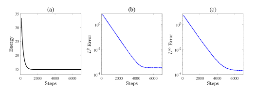
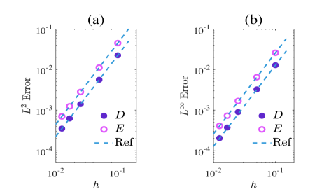
Then is the unique solution to Poisson’s equation with the -periodic boundary condition, and is the unique minimizer of the Poisson energy functional For a finite-difference grid with grid size for some , we denote by the finite-difference displacement that minimizes the discrete energy . We also denote by the iterates produced by the local algorithm. Figure 6.1 plots the discrete energy , -error , and -error vs. the iteration step of local update with the grid size . We observe a fast decrease of the energy at the beginning of iteration and then slow decrease of the energy afterwards. The errors converge to some values that are set by the grid size In Figure 6.2, we plot in the log-log scale the and -errors for the approximation of the exact minimizer and also for the approximation of the electric field , respectively, against the finite-difference grid size We observe the convergence rates as predicted by Theorem 4.1 and Corollary 4.1.
Test 2. The Poisson energy with a variable permittivity. We set
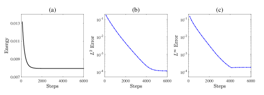
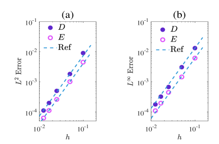
first for and then extend them -periodically to Note that is a -function. We then define and So, is the periodic solution to Poisson’s equation and is the minimizer of As in Test 1, for a finite-difference grid with grid size for some , we denote by the finite-difference displacement that minimizes the discrete energy . We also denote by the iterates produced by the local algorithm with shift. Figure 6.3 plots the discrete energy , -error , and -error vs. the iteration step of local update with the grid size . We again observe a fast decrease of the energy at the beginning of iteration and then slow decrease of the energy afterwards. The errors converge to some values that are set by the grid size In Figure 6.4, we plot in the log-log scale the and errors for the approximation of the exact minimizer and also for the approximation of the electric field , respectively, against the finite-difference grid size We observe the convergence rate as predicted by Theorem 4.1 and Corollary 4.1.
Test 3: The Poisson–Boltzmann (PB) energy with a variable permittivity. We define , , and
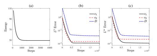
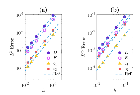
where Note that we do not need to compute the integral that defines . It can be verified that is the unique periodic solution to the CCPBE (2.11), Moreover, is the unique minimizer of For a given finite-difference grid of size , we denote by the unique minimizer of the discrete PB energy functional . We also denote by the iterates produced by the local algorithm. Figure 6.5 plots the discrete energy , -errors and , and -errors and , vs. the iteration step of local update with . We observe the monotonic decrease of all the energy and errors. In fact, the errors converge to some values that are set by the grid size In Figure 6.6, we plot in the log-log scale the and errors for the approximation of and of , and also the approximation of the electric field , respectively, against the finite-difference grid size We observe the convergence rate as predicted by Theorem 4.2 and Corollary 4.2.
Appendix
Proof of Lemma 3.1.
The first discrete Green’s identity follows from an application of summation by parts and the periodicity. The second identity follows from the first one.
Let us use the symbol instead of to denote the imaginary unit: For each grid point we define by
The system is an orthonormal basis for the space of all complex-valued, -periodic, grid functions with respect to the inner product defined in (3.1).
Let be -periodic and satisfy Since is a constant function and , we have
where denotes the sum over all such that and Hence,
Consequently, since are orthonormal, we have
where we used the identity Calculations for the differences and are similar.
It now follows from (3.2) and the definition of that
Note that and that if Hence, if , then Finally, we have
leading to the desired inequality. ∎
Acknowledgment
This work was supported in part by the US National Science Foundation through the grant DMS-2208465 (BL), the National Natural Science Foundation of China through the grant 12171319 (SZ). The authors thank Professor Burkhard Dünweg for helpful discussions and thank Professor Zhenli Xu for his interest in and support to this work. BL and QY thank Professor Zhonghua Qiao for hosting their visit to The Hong Kong Polytechnic University in the summer of 2023 where this work was initiated.
References
- [1] R. Adams. Sobolev Spaces. Academic Press, New York, 1975.
- [2] D. Andelman. Electrostatic properties of membranes: The Poisson–Boltzmann theory. In R. Lipowsky and E. Sackmann, editors, Handbook of Biological Physics, volume 1, pages 603–642. Elsevier, 1995.
- [3] N. A. Baker, D. Sept, S. Joseph, M. J. Holst, and J. A. McCammon. Electrostatics of nanosystems: Application to microtubules and the ribosome. Proc. Natl. Acad. Sci. USA, 98:10037–10041, 2001.
- [4] M. Baptista, R. Schmitz, and B. Dünweg. Simple and robust solver for the Poisson–Boltzmann equation. Phys. Rev. E, 80:016705, 2009.
- [5] J. T. Beale. Smoothing properties of implicit finite difference methods for a diffusion equaiton in maximum norm. SIAM J. Numer. Anal., 47(4):2476–2495, 2009.
- [6] D. L. Chapman. A contribution to the theory of electrocapillarity. Phil. Mag., 25:475–481, 1913.
- [7] J. Che, J. Dzubiella, B. Li, and J. A. McCammon. Electrostatic free energy and its variations in implicit solvent models. J. Phys. Chem. B, 112:3058–3069, 2008.
- [8] T. A. Darden, D. M. York, and L. G. Pedersen. Particle mesh Ewald: an method for Ewald sums in large systems. J. Chem. Phys., 98:10089–10092, 1993.
- [9] M. E. Davis and J. A. McCammon. Electrostatics in biomolecular structure and dynamics. Chem. Rev., 90:509–521, 1990.
- [10] S. W. de Leeuw, J. W. Perram, and E. R. Smith. Simulation of electrostatic systems in periodic boundary conditions. I. Lattice sums and dielectric constants. Proc. R. Soc. Lond. A, 373:27–56, 1980.
- [11] S. W. de Leeuw, J. W. Perram, and E. R. Smith. Simulation of electrostatic systems in periodic boundary conditions. II. Equivalence of boundary conditions. Proc. R. Soc. Lond. A, 373:57–66, 1980.
- [12] P. Debye and E. Hückel. Zur theorie der elektrolyte. Physik. Zeitschr., 24:185–206, 1923.
- [13] L. C. Evans. Partial Differential Equations, volume 19 of Graduate Studies in Mathematics. Amer. Math. Soc., 2nd edition, 2010.
- [14] P. P. Ewald. Die berechnung optischer und elektrostatischer gitterpotentiale. Ann. Phys., 369(3):253–287, 1921.
- [15] M. Fixman. The Poisson–Boltzmann equation and its applications to polyelectrolytes. J. Chem. Phys., 70(11):4995–5005, 1979.
- [16] F. Fogolari, A. Brigo, and H. Molinari. The Poisson–Boltzmann equation for biomolecular electrostatics: a tool for structural biology. J. Mol. Recognit., 15:377–392, 2002.
- [17] D. Frenkel and B. Smit. Understanding Molecular Simulation: From Algorithms to Applications. Academic Press, 1996.
- [18] D. Gilbarg and N. S. Trudinger. Elliptic Partial Differential Equations of Second Order. Springer–Verlag, 2nd edition, 1998.
- [19] M. Gouy. Sur la constitution de la charge électrique a la surface d’un électrolyte. J. Phys. Théor. Appl., 9:457–468, 1910.
- [20] P. Grochowski and J. Trylska. Continuum molecular electrostatics, salt effects and counterion binding—A review of the Poisson–Boltzmann model and its modifications. Biopolymers, 89:93–113, 2008.
- [21] B. Hille. Ion Channels of Excitable Membranes. Sinauer Associates, 3rd edition, 2001.
- [22] B. Honig and A. Nicholls. Classical electrostatics in biology and chemistry. Science, 268:1144–1149, 1995.
- [23] J. D. Jackson. Classical Electrodynamics. Wiley, New York, 3rd edition, 1999.
- [24] L. D. Landau, E. M. Lifshitz, and L. P. Pitaevski. Electrodynamics of Continuous Media. Butterwort-Heinemann, 2nd edition, 1993.
- [25] C.-C. Lee. The charge conserving Poisson–Boltzmann equations: Existence, uniqueness, and maximum principle. J. Math. Phys., 55:051503, 2014.
- [26] B. Li. Continuum electrostatics for ionic solutions with nonuniform ionic sizes. Nonlinearity, 22:811–833, 2009.
- [27] B. Li. Minimization of electrostatic free energy and the Poisson–Boltzmann equation for molecular solvation with implicit solvent. SIAM J. Math. Anal., 40:2536–2566, 2009.
- [28] B. Li., X.-L. Cheng, and Z.-F. Zhang. Dielectric boundary force in molecular solvation with the Poisson–Boltzmann free energy: A shape derivative approach. SIAM J. Appl. Math., 71(10):2093–2111, 2011.
- [29] B. Li, P. Liu, Z. Xu, and S. Zhou. Ionic size effects: Generalized Boltzmann distributions, counterion stratification, and modified Debye length. Nonlinearity, 26:2899–2922, 2013.
- [30] J. Li and S. Shields. Superconvergence analysis of Yee scheme for metamaterial Maxwell’s equations on non-uniform rectangular meshes. Numer. Math., 134:741–781, 2016.
- [31] S. Liu, Z. Zhang, H.-B. Cheng, L.-T. Cheng, and B. Li. Explicit-solute implicit-solvent molecular simulation with binary level-set, adaptive-mobility, and GPU. J. Comput. Phys., 472:111673, 2023.
- [32] A. C. Maggs. Dynamics of a local algorithm for simulating Coulomb interactions. J. Chem. Phys., 117(5):1975–1981, 2002.
- [33] A. C. Maggs and V. Rossetto. Local simulation algorithms for Coulomb interactions. Phys. Rev. Lett., 88:196402, 2002.
- [34] P. Monk and E. Süli. A convergence analysis of Yee’s scheme on nonuniform grids. SIAM J. Numer. Anal., 31(2):393–412, 1994.
- [35] I. Pasichnyk and B. Dünweg. Coulomb interactions via local dynamics: A molecular-dynamics algorithm. J. Phys.: Condens. Matter, 16:S3999, 2004.
- [36] M. Pruitt. Large time step maximum norm regularity of L-stable difference methods for parabolic equations. Numer. Math., 128:551–587, 2014.
- [37] M. Pruitt. Maximum norm regularity of periodic elliptic difference operators with variable coefficients. ESAIM: Math. Model. Numer. Anal., 49:1451–1461, 2015.
- [38] Z. Qiao, Z. Xu, Q. Yin, and S. Zhou. A Maxwell-Ampère Nernst-Planck framework for modeling charge dynamics. SIAM J. Appl. Math., 83:374–393, 2023.
- [39] Z. Qiao, Z. Xu, Q. Yin, and S. Zhou. Structure-preserving numerical method for Maxwell-Ampère Nernst-Planck model. J. Comput. Phys., 475:111845, 2023.
- [40] Z. Qiao, Z. Xu, Q. Yin, and S. Zhou. Local structure-preserving relaxation method for equilibrium of charged systems on unstructured meshes. SIAM J. Sci. Comput., 46(4):A2248–A2269, 2024.
- [41] J. Rauch and L. R. Scott. The charge-group summation method for electrostatics of periodic crystals. SIAM J. Appl. Math., 81(2):694–717, 2021.
- [42] J. B. Rauch and L. R. Scott. The electrostatic potential of periodic crystals. SIAM J. Math. Anal., 53:1474–1491, 2021.
- [43] P. Ren, J. Chun, D. G. Thomas, M. J. Schnieders, M. Marucho, J. Zhang, and N. A. Baker. Biomolecular electrostatics and solvation: a computational perspective. Quarterly Rev. Biophys., 45:427–491, 2012.
- [44] J. Rottler and A. C. Maggs. Local molecular dynamics with Coulombic interactions. Phys. Rev. Lett., 93(17):170201, 2004.
- [45] K. A. Sharp and B. Honig. Calculating total electrostatic energies with the nonlinear Poisson–Boltzmann equation. J. Phys. Chem., 94:7684–7692, 1990.
- [46] R. Temam. Navier–Stokes Equations: Theory and Numerical Analysis. North-Holland, 3rd edition, 1984.
- [47] J. M. Varah. A lower bound for the smallest singular value of a matrix. Linear Algebra Appl., 11:3–5, 1975.
- [48] R. S. Varga. On diagonal dominance arguments for bounding . Linear Algebra Appl., 14:211–217, 1976.
- [49] K. Yee. Numerical solution of initial boundary value problems involving Maxwell’s equations in isotropic media. IEEE Trans. Antennas and Propagation, 14(3):302–307, 1966.
- [50] Z. Zhang and L.-T. Cheng. Binary level-set method for variational implicit solvation model. SIAM J. Sci. Comput., 45:B618–B645, 2023.
- [51] Z. Zhang, C. G. Ricci, C. Fan, L.-T. Cheng, B. Li, and J. A. McCammon. Coupling Monte Carlo, variational implicit solvation, and binary level-set for simulations of biomolecular binding. J. Chem. Theory Comput., 17:2465–2478, 2021.
- [52] H.-X. Zhou. Macromolecular electrostatic energy within the nonlinear Poisson–Boltzmann equation. J. Chem. Phys., 100:3152–3162, 1994.
- [53] S. Zhou, L.-T. Cheng, J. Dzubiella, B. Li, and J. A. McCammon. Variational implicit solvation with Poisson–Boltzmann theory. J. Chem. Theory Comput., 10:1454–1467, 2014.
- [54] S. Zhou, Z. Wang, and B. Li. Mean-field description of ionic size effects with non-uniform ionic sizes: A numerical approach. Phys. Rev. E, 84:021901, 2011.