Improving behavior profile discovery for vehicles

Abstract

Multiple approaches have already been proposed to mimic real driver behaviors in simulation. This article proposes a new one, based solely on the exploration of undisturbed observation of intersections. From them, the behavior profiles for each macro-maneuver will be discovered. Using the macro-maneuvers already identified in previous works, a comparison method between trajectories with different lengths using an Extended Kalman Filter (EKF) is proposed, which combined with an Expectation-Maximization (EM) inspired method, defines the different clusters that represent the behaviors observed. This is also paired with a Kullback-Liebler divergent (KL) criteria to define when the clusters need to be split or merged. Finally, the behaviors for each macro-maneuver are determined by each cluster discovered, without using any map information about the environment and being dynamically consistent with vehicle motion. By observation it becomes clear that the two main factors for driver’s behavior are their assertiveness and interaction with other road users.

I INTRODUCTION

To predict and model interactions of road users during the driving task is still a challenging necessity for automated vehicles (AVs). Different reasons can influence road users’ behavior, producing trajectories that are ultimately distinct from each other. Since the DARPA challenges and the resurgence of AVs as a real technology, multiple methods have been proposed to model road user behaviors and thus make the AV more aware and responsive during driving. Starting from the raw data obtained by the observation of undisturbed intersections, an approach to discover vehicle behaviors in urban conditions is proposed in this work: to extract all differentiable behavior from real data using the longitudinal dynamic information (velocity and acceleration) as the main discriminator.

Given that a sufficient amount of trajectory samples have been observed, the behaviors detected from clustering the set of samples from a single maneuver should represent the totality of the probable behaviors in a specific scenario. They can be used to increase the accuracy and reduce complexity during the prediction of vehicle behavior [1], to compare if an AV generated trajectory is similar to a real one (to avoid trajectories that might startle other drivers) or to power the simulation of agents that behave and interact in a realistic manner during simulation [2]. This last one is the main motivation for the proposed work. For other fields, the general idea of the proposed method can also be useful for the dynamic analysis of human movement during a specific task, or even how different the movements of tools used/hold by surgeons are.

A particular advantage of the presented method is the discovery of every interaction mode for a maneuver, i.e., every behavior produced by a driver due to a response towards other road users (or the absence of interaction as well) is represented by one of the clusters identified. This is an extremely valuable information, obtained without any kind of hypothesis about how or why the agents interacted with others.

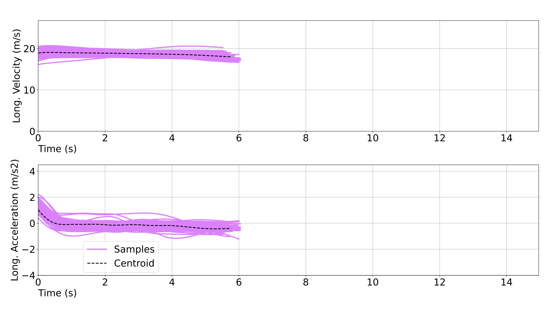
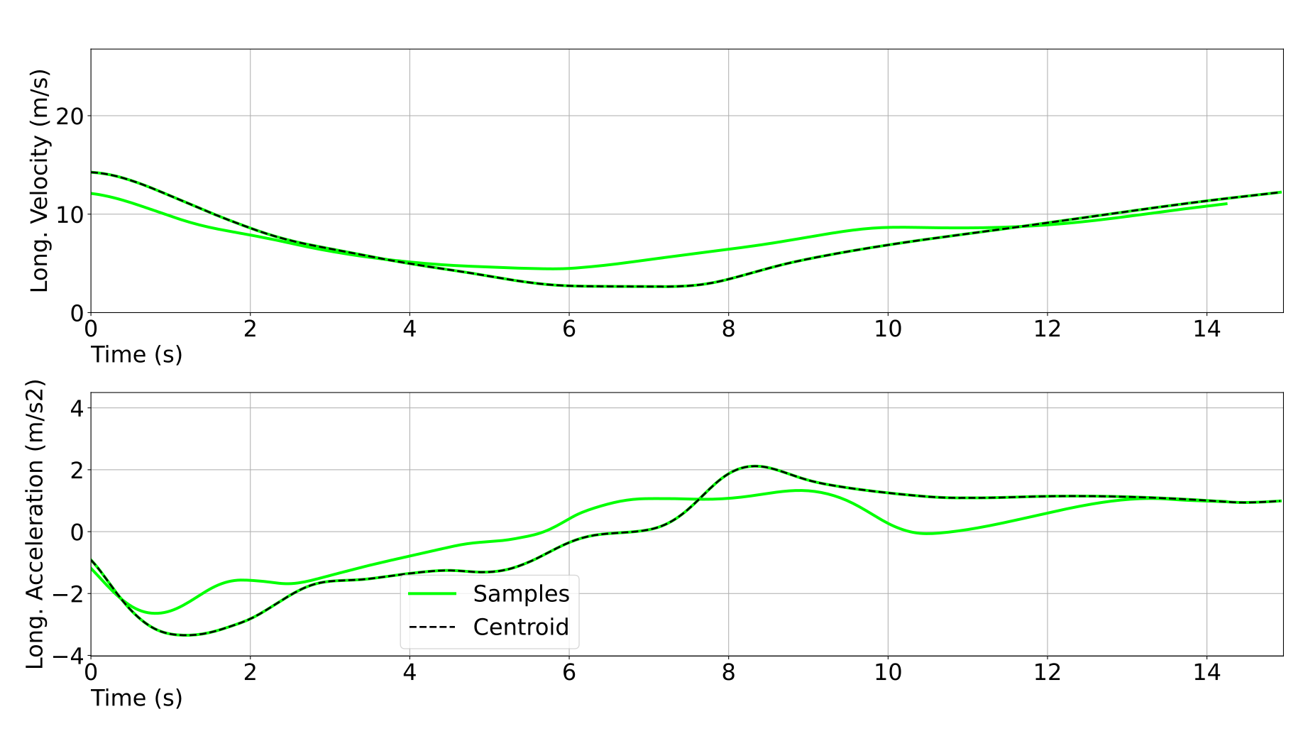
Figure 1: Lon. vel. clusters and centroid heat-maps from 9(b)

I-A Related works

There is a multitude of different motivations leading to the tentative of extracting drivers’ behaviors from raw data, for analysis of the discovered results or just to reproduce them. In [3] an inverse reinforcement learning method is used to learn driving styles from demonstration. Nine different features are considered, including jerk, acceleration, collision avoidance and lane centrality. The main goal was really to reproduce the behavior learned from multiple drivers, not to compare the differences from each driver. Another example of cluster representation approach is [4], where ensembles of trajectories represent modes of intent to be predicted.

Initial attempts to cluster together trajectories using their velocity profiles were made by proposing different comparison metrics. In the first case, [5] proposed to indirectly use the velocity during clustering with a Euclidean distance calculated in a window of points, and then applied it to a nearest neighbor and DTW algorithms. [6] actually cluster the data from different segments of a trajectory to predict the future velocity profile and try to optimize fuel consumption; which is similar to [7], with the only difference that the latter also uses the longitudinal acceleration for the clustering. However, it is known that these kind of methods are not capable of separating the profiles efficiently, as it will be shown in the results. Similar methods can also be seen in [8], where a complete trajectory is separated in parts and then clustered with a DBSCAN-inspired approach. A more complete review of metric methods can be found in [9] and [10].

There are two other general approaches for driver behavior discovery: probabilistic-based and learning-based. In [11], a mixture of Hidden Markov Models (HMM) is used to represent each possible behavior profile. An Expectation-Maximization (EM) algorithm is then used to estimate the mixing coefficient and the parameters of each state for all HMMs. As a drawback this method could have wildly different number of clusters for similar scenarios, and also the meaning of each HMM’s state is a priori unknown. The work in [12] follows the same approach and applies the clusters to predict behaviors at intersection. Specifically, it uses a polynomial regression mixture, where an EM algorithm calculates the allocation of each sample to a specific cluster and then it optimizes the polynomial that represent the cluster’s centroid. [13] generically discover the minimal set of trajectory subsections that can represent its entirety and [14] used a variational Gaussian Mixture Model (GMM) to classify the maneuvers in a highway of the surrounding vehicles with predefined class labels and motion models.

A deep-learning approach to calculate the similarity of trajectories is proposed by [15], where an encoder-decoder architecture is trained to quantitatively evaluate the similarity of urban trajectories that might present noise, missing points or different sampling frequencies; however, this comparison uses a higher view-scale than the one needed in this article. In [16] an end-to-end clustering approach is presented, improving the final results in comparison with the former publication. With an architecture based on the seq2seq publication [17], three different procedures are executed by the network: the trajectory tokenization in the embedding, its reconstruction by the decoder and finally the cluster classification. Following an embedded information approach than an explicit comparison between trajectories, [18] uses two different networks to cluster the behavior of vehicles, the first one an encoder-decoder with a 3D convolution network as encoder to compact the position and time into a single representation and a second RNN-based network where the resulting hidden vector is also combined to cluster the data. And [19] produced a topological map with nine six different parameters (lateral and longitudinal velocities included) from 59 demonstrations on simulation to optimize the t-SNE representation of the results and subsequent clustering using a GMM.

All the cited methods use, in some form, the velocity into its proposed clustering, but none use the dynamic characteristics of a nonholonomic vehicle nor they separate the positional clustering influence from the inherent longitudinal profile each driver may have. Thus, the main contributions of this paper lies in the capability to cluster only the longitudinal information of vehicles to first confirm that drivers adopt a wide range of possible speed / acceleration profiles during the driving task and to (in a procedural manner) obtain such different behaviors. Section II details the similarity measure used while section III explains how the clustering is done. The results are reported in section IV.

II Dynamic analysis of longitudinal clusters

Dealing only with the longitudinal information of trajectories assumes that the data is already structured into different macro-maneuvers. This is the scope considered here: all data used has been already processed into specific maneuvers detected in their respective scenarios. Figure 2 shows the maneuver 0 from scenario 0 of the InD dataset [20]. The clustering method to determine the set of trajectory samples for each maneuver was proposed in [21], which made important improvements over [7].

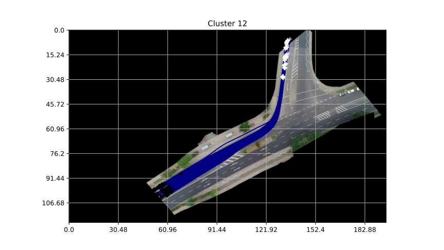
Figure 2: Example of macro-maneuver (from InD dataset [20])

II-A EKF to determine similarity

Each trajectory considered is composed by its position ($s_{x,t},s_{y,t}$), orientation ($\theta_{t}$) and the longitudinal information (velocity and acceleration, $v_{{lon}_{t}},a_{{lon}_{t}}$), as represented in equation (1), where $\mathbb{S}_{k}$ indicates the sample considered and $\mathbb{T}_{j}$ the duration of the trajectory $j$. The state vector $\bm{x}_{j}(t)$ (from now onward represented as $\bm{x}_{t}$) and the control vector $\bm{u}_{j}(t)$ ($\bm{u}_{t}$) are defined in equations (2) and (3), where $\phi_{t}$ represents the steering angle signal.

$$\bm{r}_{j}=\left[\left(s_{x,t},s_{y,t},\theta_{t},v_{\text{lon},t},a_{\text{lon},t}\right)_{j}\right],\forall t\in\mathbb{T}_{j}\text{, }j\in\mathbb{S}_{k}$$ (1)

$$\bm{x}_{j}(t) =\left[s_{x,t},s_{y,t},\theta_{t},v_{\text{lon},t}\right]$$ (2)

$$\bm{u}_{j}(t) =\left[a_{\text{lon},t},\phi_{t}\right]$$ (3)

KF-derived methods are used for prediction under the assumption that observation and measurement noises can be approximated by Gaussians [22], enabling the membership calculation from a trajectory to a certain cluster. Smoothing is also possible, since the entire trajectory is known, but unnecessary given how the EKF will be used and also the higher computational demand in comparison. Equations (4), (5) and (6) through (8) show the EKF framework, with $\bm{z}_{t}$ being the observation vector. Convergence is assured according to [23].

$$\bar{\bm{\mu}}_{t+1} =\mathcal{T}(\bm{\mu}_{t},\bm{u}_{t})$$ (4)

$$\bar{\bm{\Sigma}}_{t+1} =\bm{G}_{t+1}\bm{\Sigma}_{t}\bm{G}_{t+1}^{T}+\bm{R}$$ (5)

$$\bm{K}_{t+1} =\bar{\bm{\Sigma}}_{t+1}\bm{H}_{t+1}^{T}\cdot(\bm{H}_{t+1}\bar{\bm{\Sigma}}_{t+1}\bm{H}_{t+1}^{T}+\bm{Q})^{-1}$$ (6)

$$\bm{\mu}_{t+1} =\bar{\bm{\mu}}_{t+1}+\bm{K}_{t+1}(\bm{z}_{t+1}-\bm{h}(\bar{\bm{\mu}}_{t+1}))$$ (7)

$$\bm{\Sigma}_{t+1} =(\bm{I}-\bm{K}_{t+1}\bm{H}_{t+1})\bar{\bm{\Sigma}}_{t+1}$$ (8)

The prediction model for the task at hand, $\mathcal{T}(\bm{\mu}_{t},\bm{u}_{t})$, can be seen in (9): the kinematic bicycle model without slippage for vehicle nonholonomic movement using front-wheel driving, where $l_{j}$ is the wheelbase of the vehicle. The matrix $G$ in equation (5) is the Jacobian from equation (9) and can be seen in [24] (H as well).

$$\begin{cases}\dot{x}_{t+1}&=v_{t}\cos\theta_{t}\cos\phi_{t}\\ \dot{y}_{t+1}&=v_{t}\sin\theta_{t}\cos\phi_{t}\\ \dot{\theta}_{t+1}&=\frac{v_{t}}{l_{j}}\sin\phi_{t}\\ \dot{v}_{t+1}&=a_{\text{lon,t}}\end{cases}$$ (9)

The comparison is achieved using the trajectory from the sample being considered, $\bm{x}_{t}$, to calculate the steering angle $\phi_{t}$ and the acceleration used in $\bm{u}_{t}$ at equation 4 for the prediction step from the current cluster centroid. Multiple steps are predicted until the update, where the real centroid trajectory serves as observation.

Equations (7) and (8) are the update correction for the prediction. Since the trajectory data used here was acquired with a 25Hz system (drone camera), each data time-step takes 40ms; the EKF prediction is executed in 10ms steps (four predictions between data-points available) and it is updated every 80ms. This design choice is important to propagate the errors from a sample that should not be in the cluster being tested.

To calculate the steering angle, the controller in (10) was implemented from [25]. $k$ is the gain, $d_{\text{lat}}$ is the lateral distance between the current position and the target point, which is the next iteration point and $\theta_{\text{tr}}$ the reference direction (calculate using the current and next point of the trajectory). The controller results in a global asymptotically stable equilibrium at $d_{\text{lat}}=0$ for $v_{\text{lon,t}}>0$ and $0<(\theta_{\text{tr}}-\theta_{t})<\frac{\pi}{2}$ [25].

$$\phi_{t+1}=(\theta_{\text{tr}}-\theta_{t})+\arctan\left(\frac{k\cdot d_{\text{lat}}}{v_{\text{lon,t}}}\right)$$ (10)

II-B Membership calculation

The Mahalanobis distance $d_{M,t}$, equation (11) is calculated after a certain number of sequential predictions, creating a gap between the real centroid state and the one predicted with the sample information. As it happens, this distance is distributed according to the $\chi^{2}_{n}(\delta^{2})$ distribution [26], specifically a centered chi-squared with four degrees of liberty: $\chi^{2}_{4}$. A very practical use of this distance can be seen in [27] where it is used to verify the integrity of a region of interest to detect moving objects using a LIDAR, or in [28], using the distance to increase the robustness of the estimations done by an EKF implementation.

$$d_{M,t}^{2}=(\bm{z}_{t}-\bm{\mu}_{t})^{T}\cdot\bm{\Sigma}_{t}^{-1}\cdot(\bm{z}_{t}-\bm{\mu}_{t})\sim\bm{\chi}^{2}_{n}$$ (11)

The membership of a certain sample trajectory can then be calculated before the update step using the distance given by (11), with $z_{t}$ being the state of the centroid trajectory at the current time-step. At time $t$, the membership probability from the sample to the cluster represented by the centroid $\bm{x}_{c_{i}}$ is given by equation (12). The probability at the right side of (12) is the cumulative distribution function (c.d.f.) from $\chi^{2}_{4}$, representing the probability that the distance between the estimated state and the observed one is higher than what was obtained by the EKF.

$$p(\bm{x}_{t}\in\mathcal{C}_{i}|\bm{x}_{c_{i}})=1-p(d\geq d_{M,t}^{2})$$ (12)

As the final product of the comparison, $p(\bm{x}_{t}\in\mathcal{C}_{i}|\bm{x}_{c_{i}})$ will look something like Figure 3 for the case where the trajectory tested (in red) does not belong to the cluster whose centroid has a longitudinal velocity profile shown in blue. On the opposite, Figure 4 shows a sample trajectory that does belong to the cluster, fact made clear by the high probability calculated and displayed in purple.

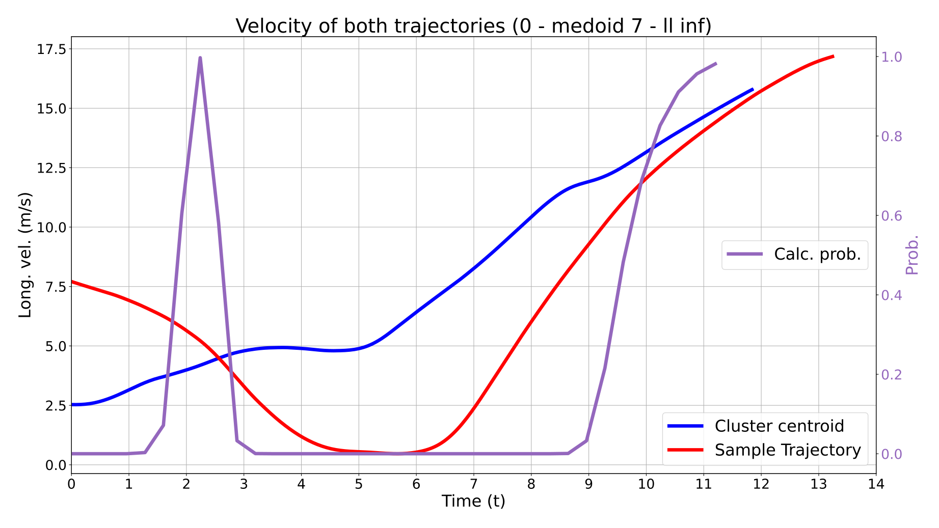
Figure 3: Two trajectories from different clusters

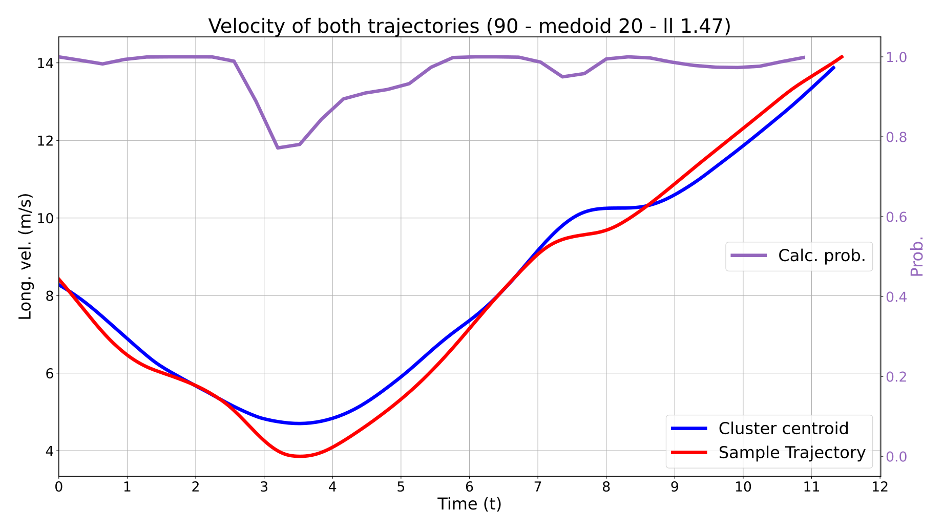
Figure 4: Two trajectories from the same cluster

III Optimizing cluster distribution

Two different quantities will be evaluated by the proposed algorithm: the number of clusters in the studied data and the similarity between each element inside the cluster, which is represented by $p(\bm{x}_{t}\in\mathcal{C}_{i}|\bm{x}_{c_{i}})\text{ , for t}\in\mathbb{T}_{j}$, the probability that at time $t$ the sample is similar to the cluster’s centroid. This membership probability is not a practical metric to work with the expectation-maximization (EM); the negative log-likelihood (equation (13)), with $\bm{x}_{c_{i}}$ being the centroid of $\mathcal{C}_{i}$ ($c_{i}$ indicating the element from $\mathcal{C}_{i}$ that is the centroid), compresses the time series into one scalar.

$$nll(\bm{x}_{j}|\bm{x}_{c_{i}})=\sum_{t=0}^{T}-\ln\left[p(\bm{x}_{t}\in\mathcal{C}_{i}|\bm{x}_{c_{i}})\right]$$ (13)

Another advantage from the equation (13) form is that if the probability at any point in time goes to zero, nll goes to infinity, thus being a clear marker that the sampled trajectory evaluated does not belong in the cluster being tested.

III-A Negative log-likelihood minimization

Following the structure of an EM method, the first step is to minimize $nll(\bm{x}_{j}|\bm{x}_{c_{i}})$ for each sample being considered using all the current centroids. Simply put, to search for the best cluster possible for each sample. Considering $p(\bm{x}_{j}\in\mathcal{C}_{i}|\bm{x}_{c_{k}})$ as the probability that the element $\bm{x}_{j}$ belongs to the cluster $\mathcal{C}_{i}$ given $\bm{x}_{c_{k}}$ as centroid, the EM algorithm consists in the expectation phase, equation (14) and the maximization step in equation 15. Firstly, the expectation of $\bm{x}_{i}$ belonging to cluster $\mathcal{C}_{i}$ given that the centroid used was $\bm{x}_{k}$ is calculated; and finally, with the cluster elements defined the calculated expectation expression is maximized by choosing the optimal centroid $\bm{x}_{k}$ for each cluster [29].

$$\mu_{ll} =\mathbb{E}_{\mathcal{C}_{i}|\bm{x}_{j},\bm{x}_{c_{k}}}\left[\ln p(\bm{x}_{j}\in\mathcal{C}_{i}|\bm{x}_{c_{k}})\right]$$ (14)

$$\bm{x}_{c_{k}} =\operatorname*{arg\,max}_{\bm{x}_{c_{k}}}\left[\mathbb{E}_{\mathcal{C}_{i}|\bm{x}_{j},\bm{x}_{c_{k}}}\ln p(\bm{x}_{j}\in\mathcal{C}_{i}|\bm{x}_{c_{k}})\right]$$ (15)

Since the EKF comparison presented in the subsection II-B calculates $p(x_{j}\in\mathcal{C}_{i}|x_{\mathcal{C}_{i}})$, this operation becomes a hard clustering (in opposition to a soft clustering like C-means, where the samples are assigned multiple partial membership probabilities instead of a single one). Hence, equation (16) displays the allocation of elements in the best cluster possible by minimizing the negative log-likelihood and equation (17) shows the selection of the new centroid by minimizing the sum of log-likelihoods from the other elements of the cluster.

$$\mathcal{C}_{k}(\bm{x}_{j}) =\operatorname*{arg\,min}_{\mathcal{C}_{k}\in\mathcal{C}}\left[-\ln p(\bm{x}_{j}\in\mathcal{C}_{k}|\bm{x}_{c_{k}})\right]\text{, }\forall\bm{x}_{j}\in\mathcal{C}_{k}$$ (16)

$$x_{c_{k}} =\operatorname*{arg\,min}_{x_{\mathcal{C}_{k}}}\left[\sum_{x_{k}}-\ln p_{t}(x_{i},\mathcal{C}_{k}|x_{c_{k}})\right]$$ (17)

From now onward the probability $p(\bm{x}_{j}\in\mathcal{C}_{k}|\bm{x}_{c_{k}})$ will be expressed by $p(\bm{x}_{j}|\bm{x}_{c_{k}})$.

III-B Splitting and merging clusters

Until this point, only half of the problem was covered, hence the uncertainty about the number of clusters needs to be addressed. At the beginning of the allocation-minimization process proposed in subsection III-A, and every time that a cluster member or more have an nll equal to infinity, it is reallocated to the next best cluster. If all possible allocations result in infinity, then another cluster is created just for this element. This is the first mechanism to change the number of clusters.

In addition, two other criteria are necessary, one to split the clusters, and another to merge them. The method that will be proposed came from the realization that one could use the Kullback-Liebler (KL) divergence (equation (18)) to compare the similarity of cluster(s) before and after splitting a cluster (or merging two), as [30] does. In (18) both $P$ and $Q$ are probability distributions defined on the same sample space.

$$D_{\text{KL}}(P||Q)=\sum_{x\in\mathcal{X}}P(x)\cdot\ln\left(\frac{P(x)}{Q(x)}\right)$$ (18)

To test if a cluster should be split in two, the elements are separated using a simplified k-means with k equal to $2$, establishing $\mathcal{C}_{k}^{[0]}$ and $\mathcal{C}_{k}^{[1]}$, equation (19). New centroids are chosen ($\mathcal{C}_{k}^{[0]^{\prime}}$ and $\mathcal{C}_{k}^{[1]^{\prime}}$) for both sets and the membership probabilities are calculated ($Q^{[0]}$ and $Q^{[1]}$). The KL divergence is applied on the distributions $\mathcal{C}_{k}^{[i]}$ and $\mathcal{C}_{k}^{[i]^{\prime}}$ in equation (21), considering that the membership probabilities are actually dependent on time, as indicated by the term $\bm{x}_{t}$ in the probability $p(\bm{x}_{t}|\bm{x}_{\mathcal{C}_{k}^{[i]^{\prime}}})$.

$$\mathcal{C}_{k} =\mathcal{C}_{k}^{[0]}+\mathcal{C}_{k}^{[1]}$$ (19)

$$D_{\text{KL}}^{t}(\mathcal{C}_{k}^{[i]}||\mathcal{C}_{k}^{[i]^{\prime}})=\\ \sum_{\bm{x}_{j}\in\mathcal{C}_{k}^{[i]}}p\left(\bm{x}_{t}|\bm{x}_{c_{k}^{[i]}}\right)\cdot\ln\left(\frac{p\left(\bm{x}_{t}|\bm{x}_{c_{k}^{[i]}}\right)}{p(\bm{x}_{t}|\bm{x}_{c_{k}^{[i]^{\prime}}})}\right)$$ (21)

Finally, if the criteria expressed by equation (22) is respected, the cluster split is accepted and consolidated into the main cluster set. $\overline{D}_{\text{KL}}$ represents the average of $D_{\text{KL}}^{t}$ calculated in equation 21.

$$\left|\overline{D}_{\text{KL}}(\mathcal{C}_{k}^{[0]^{\prime}}||\mathcal{C}_{k}^{[0]})-\overline{D}_{\text{KL}}(\mathcal{C}_{k}^{[1]^{\prime}}||\mathcal{C}_{k}^{[1]})\right|\geq t_{\text{KL}}$$ (22)

The same procedure is done with the merging check-up, but with the value calculated by equation (22) being smaller than the threshold $t_{\text{KL}}$. At the end of the execution loop for equations (16) and (17), all the resulting clusters are tested to check if the pairs that are most similar (nll between their centroids) should be merged. If no changes are detected, the split hypothesis is tested (as depicted in Figure 5), and if there is change, then the EM algorithm is run again. The clustering ends when there are no changes after checking for the split and the merge of all clusters.

Figure 5: Clustering architecture proposed

IV RESULTS AND DISCUSSION

IV-A Methodology

The code used to implement and test the methods proposed was done in Python using scikit-learn and numpy. All calculations were done using a AMD 7950X processor. The noise parameters for the EKF are displayed in equations (23) and (24); the trajectories were obtained from InD dataset scenario 0 (data-batches 00 to 06).

$$R =\begin{bmatrix}0.01&0.01&0.005&0.01\end{bmatrix}\cdot I_{4}$$ (23)

$$Q =\begin{bmatrix}0.05&0.05&0.01&0.1\end{bmatrix}\cdot I_{4}$$ (24)

IV-B Analyzing the common clustering result

In light of this new method to obtain vehicles’ behaviors, the final results from [7] need to be checked. Table I shows the evaluation using the average DB score proposed in [21] and the number of infinite nll clusters.

TABLE I: Results using [7] clustering for maneuver 0

$n_{k}$ Avg. DB nb. inf. nll. $n_{k}$ Avg. DB nb. inf. nll. 2 1.38 74 16 0.7 47 3 0.92 68 17 0.72 33 4 0.90 68 18 0.68 33 8 0.81 71 22 0.64 42 9 0.78 72 23 0.65 41 10 0.83 48 24 0.65 41 13 0.76 48 27 0.67 39 14 0.69 48 28 0.60 40 15 0.71 48 29 0.61 40

There are 146 trajectories for this maneuver, displayed in Figure 2. For any value of $n_{k}$ tested no less than 33 points were considered as having infinite nll, meaning that the distance metric chosen for the clustering is not capable to capture the differences between trajectories. According to the DB score used the optimal number of clusters is 28, but this can be considered as an effect of the high cluster count, not a better clustering since the score decreases progressively with the increase of $n_{k}$.

In Figure 6 one of the worst cases from the agglomerative clustering can be seen ($n_{k}=20$), and it is clear that there are multiple behaviors merged in this simple cluster.

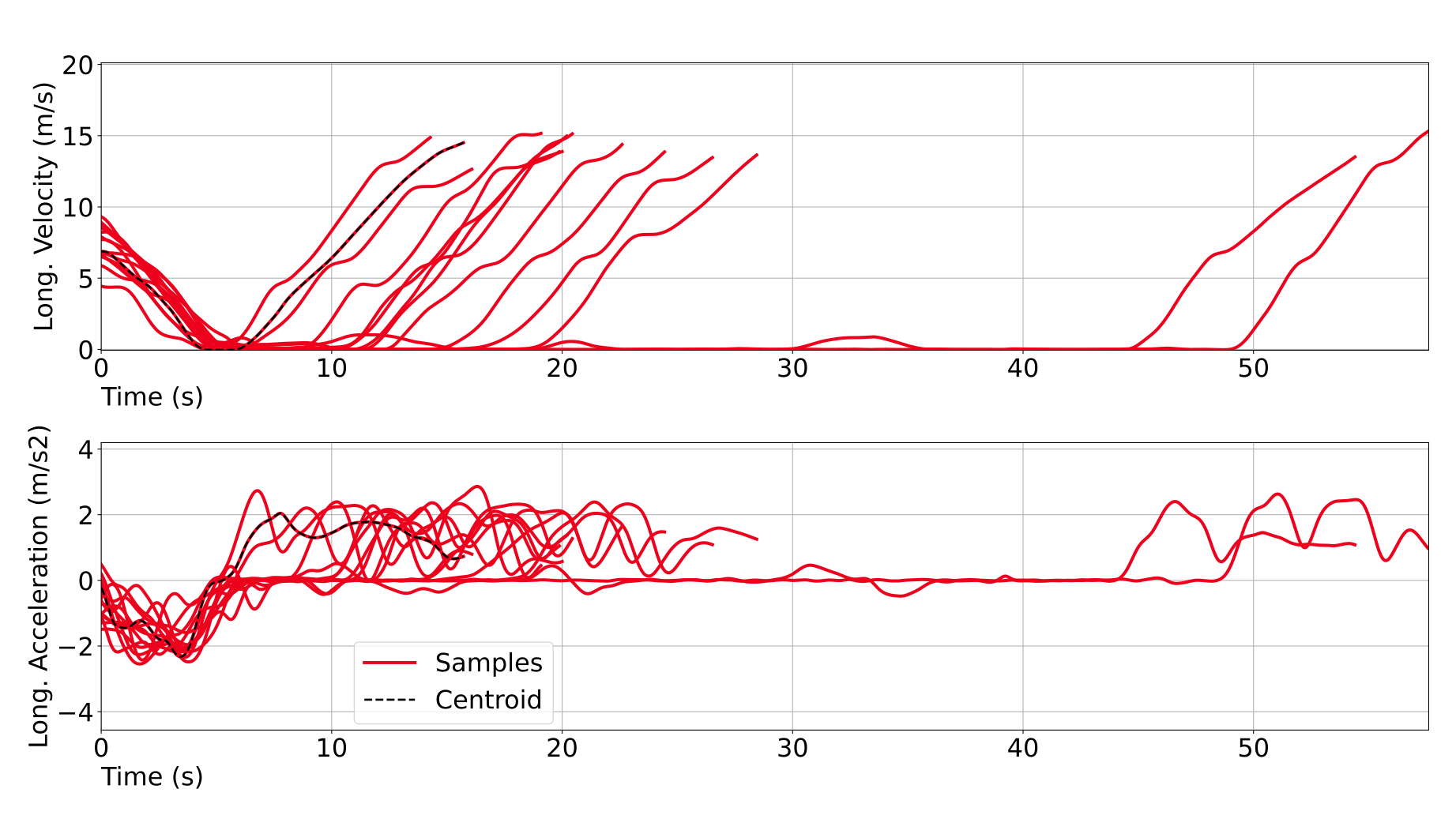
Figure 6: One of the clusters obtained with $n_{k}$ equal to 20 for maneuver 0 using the agglo. clustering

IV-C Full redistribution of samples

Due to space constraints, the analysis will be restricted to only a few maneuvers, starting with the one shown in Figure 2. The methods proposed in sections III and IV depends upon two parameters: the initial clustering organization and the split-merge threshold, $t_{KL}$. As a starting point for the algorithm, four different clustering results were used, obtained with four methods: agglomerative clustering, partition around medoids, dissimilarity matrix clustering [7] and spectral clustering, together with an $t_{KL}$ equal to $4$ and different number of initial clusters, $n^{i}_{k}$. All trajectories were rectified to start and to end at approximately similar points. This allows the algorithm to concentrate on the common parts of each trajectory, and avoid any detection problems from the original video source (from the InD dataset). The symbol $\mu_{ll}$ represents the average nll from all clusters (and $\sigma_{ll}$ the standard deviation) and $n_{k}^{f}$ the final number of clusters after execution (Figure 5).

The best result came from the initial $n_{k}$ equal to 9 from the PAM because it has the lowest $\mu_{ll}$ + $\sigma_{ll}$. It can be seen that there is still an influence from the clustering method as both the starting point and the parameter $t_{KL}$ have an importance on deciding the tightness of each cluster (lower values means more clusters).

TABLE II: Clustering results for maneuver 0 ($n_{k}^{i}$ being the initial $n_{k}$ and $n_{k}^{f}$ the final one)

$n_{k}^{i}$ $\mu_{ll}$ $\sigma_{ll}$ $n_{k}^{f}$ $n_{k}^{i}$ $\mu_{ll}$ $\sigma_{ll}$ $n_{k}^{f}$ $n_{k}^{i}$ $\mu_{ll}$ $\sigma_{ll}$ $n_{k}^{f}$ Agglomerative clustering 2 27.32 38.02 32 6 27.01 41.14 33 10 35.11 49.58 25 3 27.74 41.84 33 7 31.92 43.64 27 11 35.80 50.01 26 4 34.59 46.71 26 8 29.68 42.43 30 12 38.72 55.13 24 5 33.13 46.44 28 9 32.00 43.77 28 - - - - Partition around Medoids (PAM) 2 37.16 51.50 23 6 29.68 41.17 30 10 37.47 50.10 23 3 39.01 53.84 23 7 33.60 48.32 27 11 37.07 50.40 23 4 33.81 43.20 27 8 32.12 42.61 28 12 32.45 56.14 29 5 29.78 44.38 29 9 27.96 33.59 30 - - - - Dissimilarity matrix k-means 2 31.02 43.52 29 6 31.64 42.46 28 10 26.88 39.07 31 3 37.84 48.91 25 7 36.51 49.76 25 11 31.60 43.57 28 4 36.92 53.99 24 8 39.20 51.69 23 12 27.86 46.26 32 5 32.32 42.87 27 9 35.56 50.62 25 - - - - Spectral clustering 2 38.20 52.11 23 6 29.36 40.66 31 10 29.87 42.07 30 3 30.35 43.24 30 7 36.29 50.88 25 11 34.04 48.03 26 4 30.68 43.37 29 8 34.61 48.27 26 12 34.88 46.51 25 5 41.56 50.94 24 9 35.67 45.55 26 - - - -

Three of the clusters are presented in Figure 7 together with their centroids longitudinal velocity in Figure 8 (please refer to the digital version for a better visualization). The differences in velocity between each cluster are clear in the Figure 8, the right most plot displaying a vehicle that stopped before crossing while the leftmost plot shows a direct trajectory, without any interaction. An in-between behavior is presented by the middle plot, reduction in speed but without stopping.

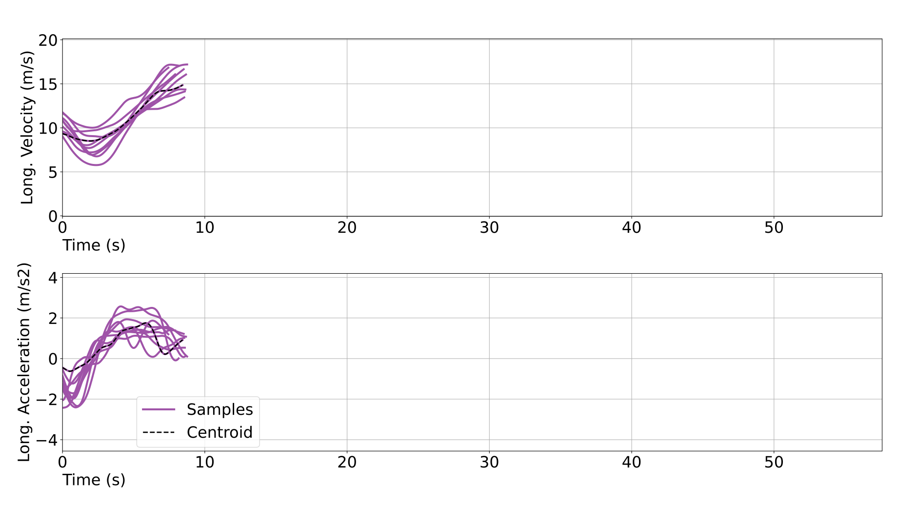
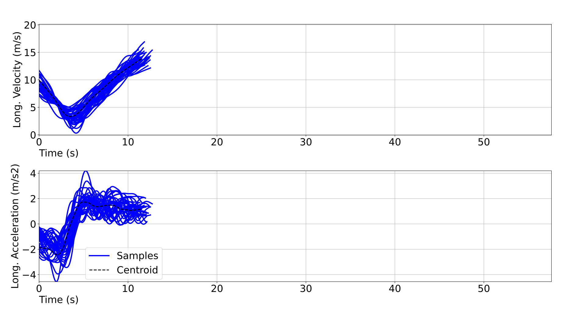
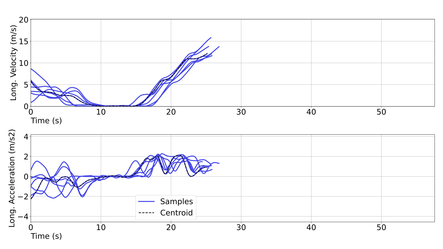
Figure 7: Four clusters from maneuver 0 result

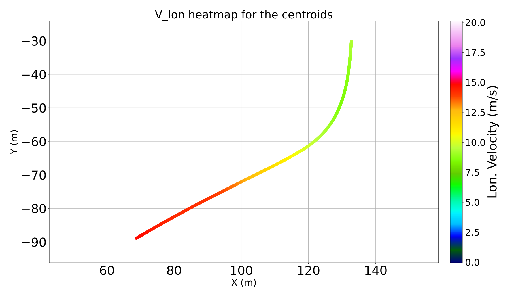
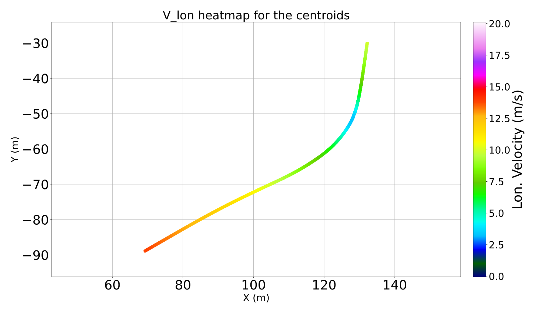
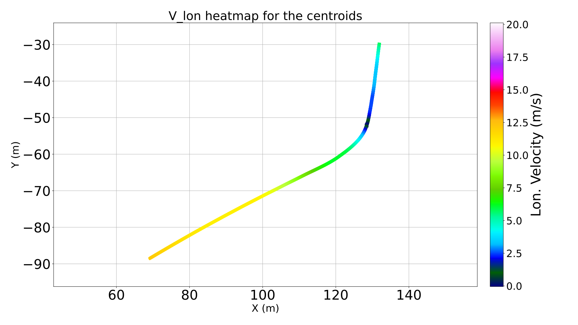
Figure 8: Lon. velocity for the centroids from Figure 7

Two other maneuvers were tested: a turn left (Figure 9(a)) and a straight maneuver (Figure 9(b)). For the turn left the results for the agglomerating starting point are displayed in Table III and two specific clusters are shown in Figure 10.

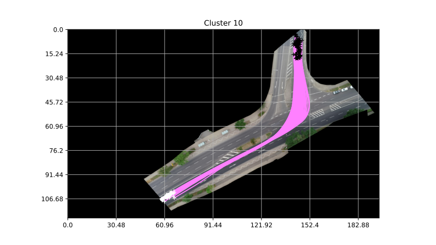
(a) Turn left maneuver

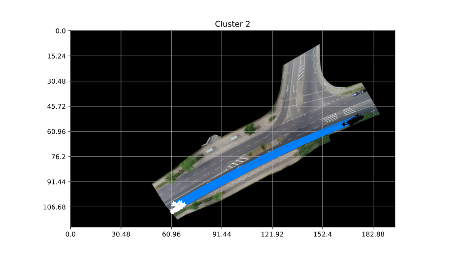
(b) Straight maneuver

Figure 9: Additional maneuvers from scenario 0

TABLE III: Results for the turn left maneuver

$n_{k}^{i}$ $\mu_{ll}$ $\sigma_{ll}$ $n_{k}^{f}$ $n_{k}^{i}$ $\mu_{ll}$ $\sigma_{ll}$ $n_{k}^{f}$ $n_{k}^{i}$ $\mu_{ll}$ $\sigma_{ll}$ $n_{k}^{f}$ 2 22.70 36.63 23 6 23.35 35.56 22 10 29.81 59.96 21 3 23.61 35.24 23 7 35.53 56.08 16 11 21.90 41.26 26 4 29.19 43.63 19 8 39.26 76.56 15 12 24.88 43.00 22 5 27.41 42.60 20 9 39.52 56.61 14 - - - -

In Figure 10(a) all samples stopped before crossing the intersection. Opposite to this behavior, Figure 10(b) displays trajectories that continue only reducing their speed to execute the turn left maneuver.

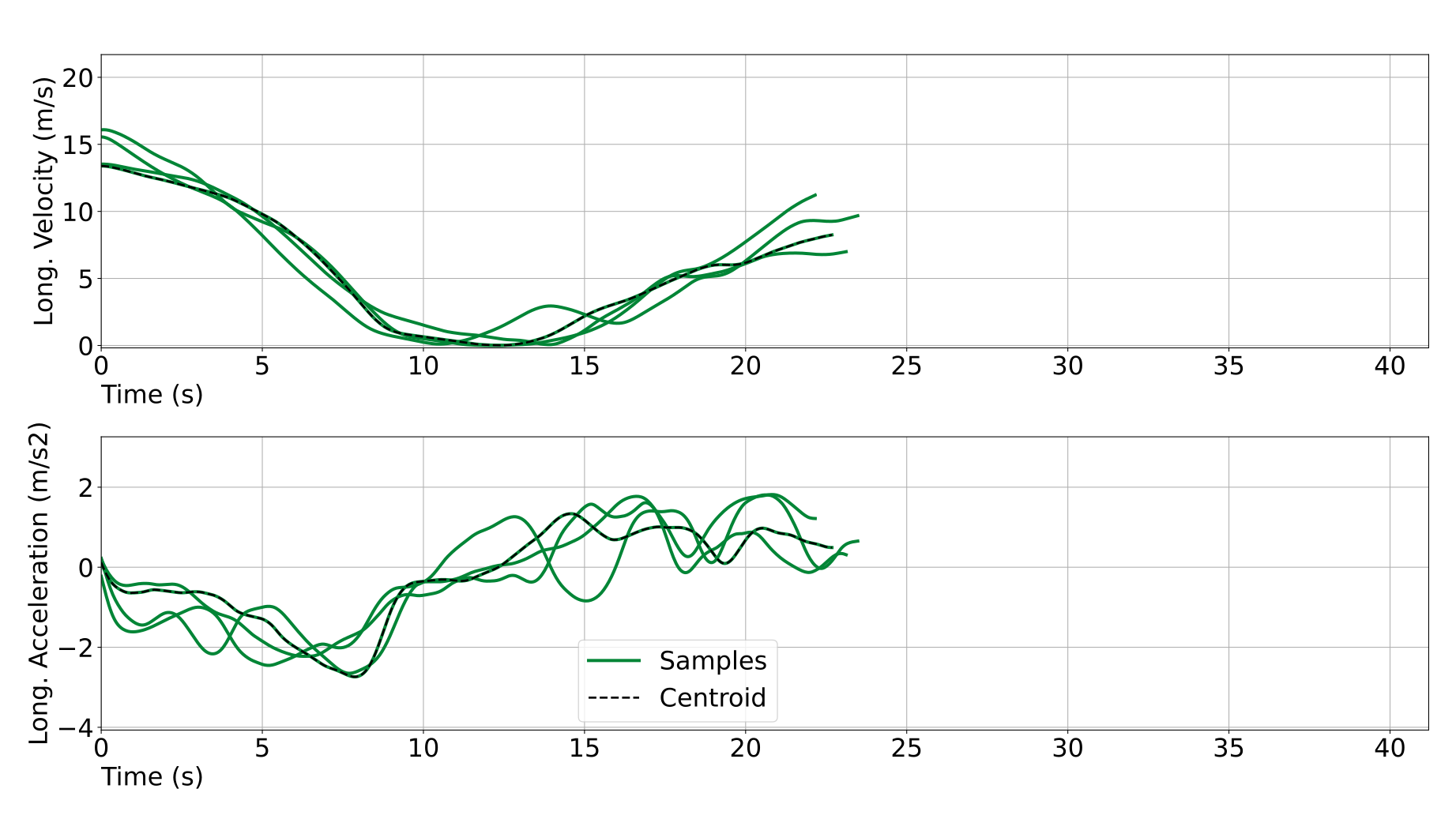
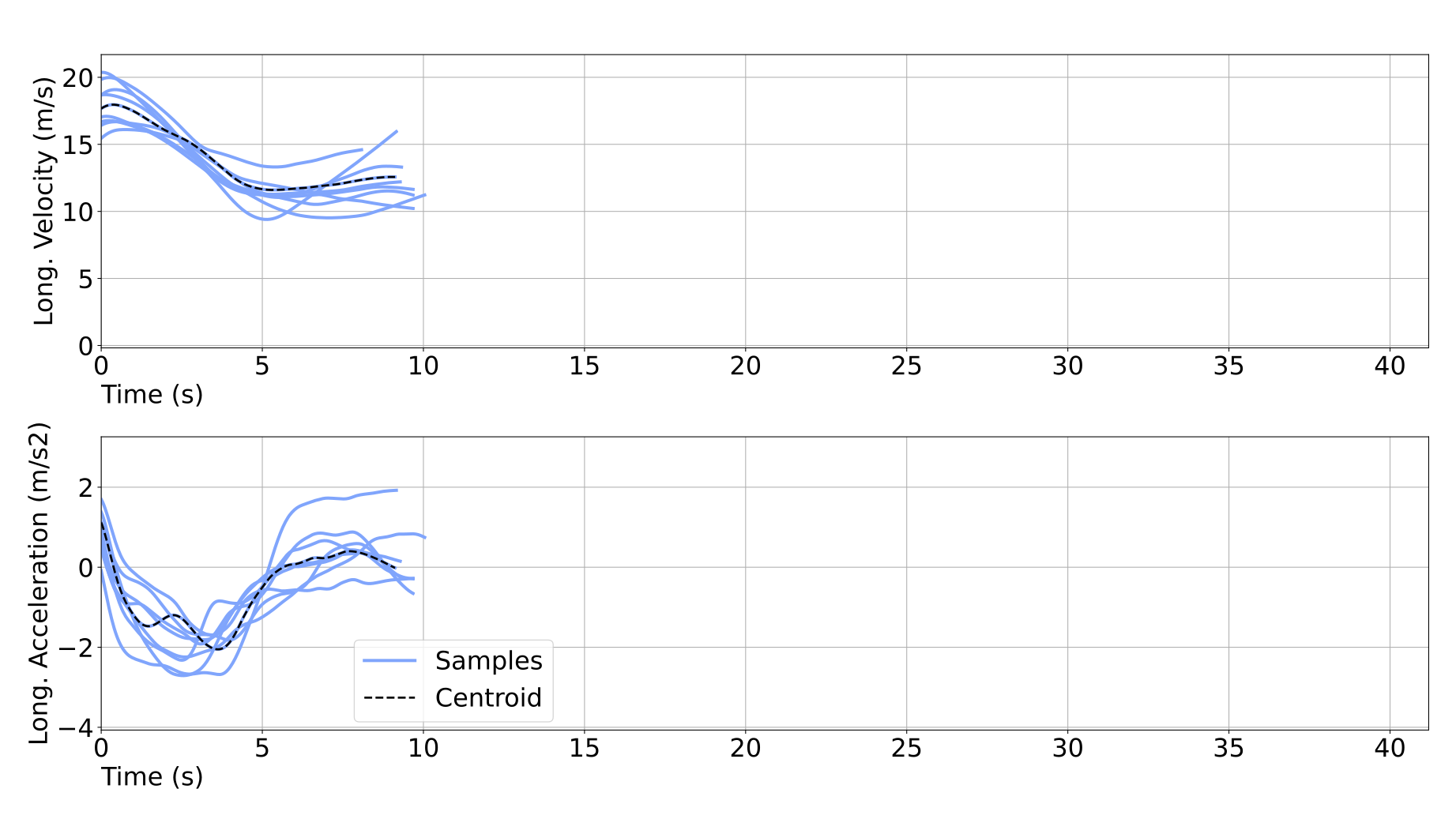
(a) Stop before crossing

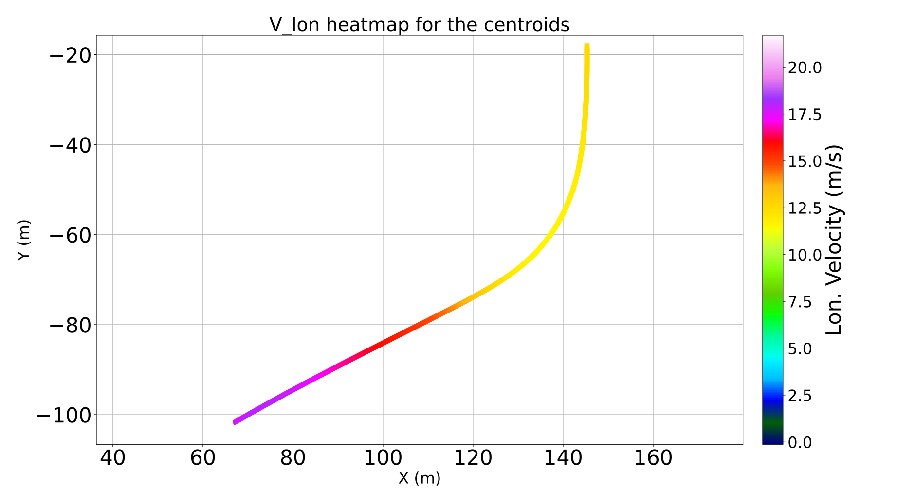
(b) Crossed directly

Figure 10: Lon. velocity profiles and heat-maps from 9(a)

There is no lack of samples for the maneuver in Figure 9(b), containing 532 trajectories. But in this case the agglomerative starting point could not differentiate between the longitudinal characteristics, which made the job of optimize the clustering and determining the best number of clusters a lot harder. The agglomerative method starting point that had the best DB score (8 clusters) was mostly concentrated into one single cluster (541 samples) and the rest only containing one or two samples. Due to this difficulty, the spectral method presented a better starting point for the clustering (Table IV).

TABLE IV: Results for the straight maneuver

$n_{k}^{i}$ $\mu_{ll}$ $\sigma_{ll}$ $n_{k}^{f}$ $n_{k}^{i}$ $\mu_{ll}$ $\sigma_{ll}$ $n_{k}^{f}$ $n_{k}^{i}$ $\mu_{ll}$ $\sigma_{ll}$ $n_{k}^{f}$ Agglomerative clustering 2 4.78 12.98 11 6 5.07 11.41 11 10 4.88 10.23 11 3 3.71 13.21 12 7 5.14 9.51 11 11 3.99 9.85 12 4 4.25 10.08 12 8 7.00 14.89 9 12 4.39 12.03 11 5 5.04 11.26 11 9 5.41 14.39 12 - - - - Spectral clustering 2 5.07 11.41 11 6 3.79 12.50 13 10 4.80 10.80 11 3 2.96 7.32 14 7 3.07 9.05 14 11 5.26 14.49 10 4 5.47 15.60 10 8 6.67 12.84 10 12 4.14 12.92 11 5 7.97 14.38 8 9 9.23 17.20 8 - - - -

The best result according to Table IV was the $n_{k}$ equal to 3. There is a predilection for the spectral cluster initialization for straight line maneuvers actually, since the same type of result was observed for other maneuvers of the same type. As an example, Figure 1 shows two clusters in different extremes, one with high speed and another with a continuous breaking.

IV-D Grouping trajectories in semantic significant behavior

Assuming that the behavior profiles obtained via the clustering discussed are mostly influenced by the assertiveness of a road user and what interaction it describes, all clusters can be structured in function of one of these factors. For the turn left maneuver from Figure 2, all the profiles obtained in Table III (30 clusters) are separated using the centroids obtained previously.

(a) Assertiveness profiles

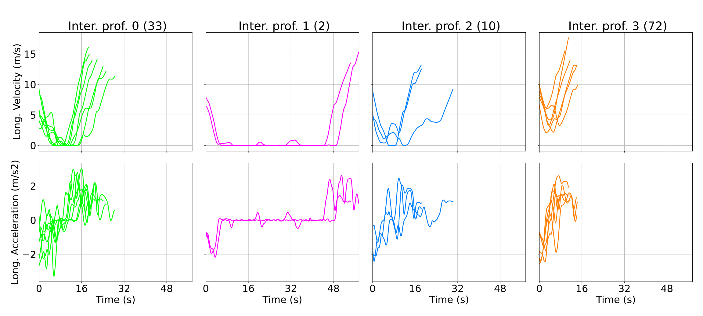
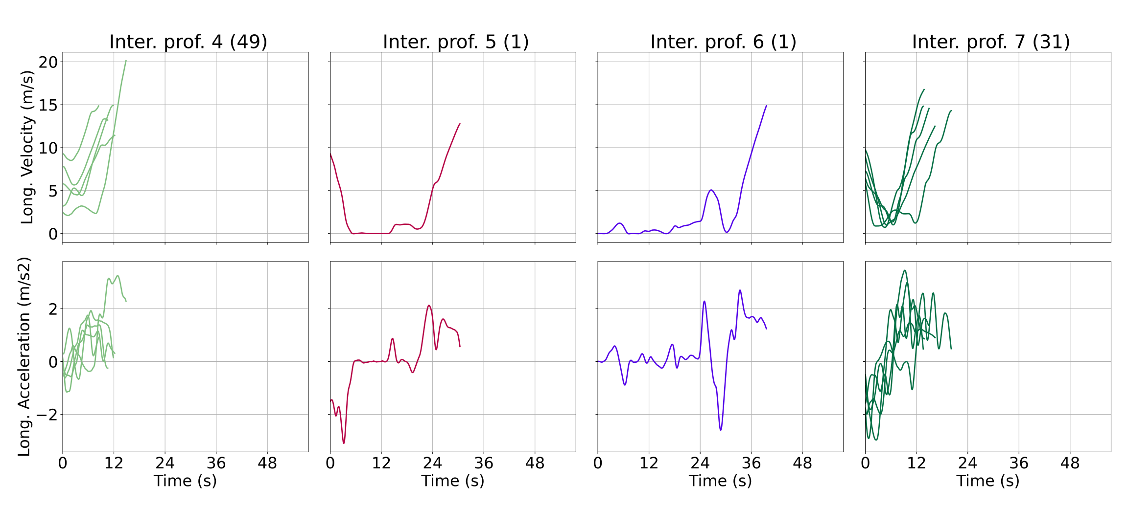
(b) Interaction profiles

Figure 11: Behavior profiles for turn right

Two clustering operations are executed with the centroids, with a fixed $n_{k}^{a}$ for the assertiveness and a certain number of interaction clusters, $n_{k}^{i}$, where $n_{k}^{a}\cdot n_{k}^{i}=n_{k}-c$ ($c$ adjusts the multiplication, all pairings are necessarily observed). There are 30 optimal clusters, defining 4 different assertiveness profiles and 8 interaction ones. The assertiveness clustering was done using three features: the initial longitudinal velocity, the period in witch the longitudinal acceleration stayed below -2 $m/s^{2}$, and lastly, above 1.5 $m/s^{2}$. These three features were normalized and clustered using the agglomeration algorithm, resulting in the Figure 11(a).

All clusters contain a range of different interactions, from slowing down to turn to stop altogether. As expected, the cluster that have a more aggressive result starts with a higher velocity and/or has a higher absolute acceleration while all behaviors on the conservative class got close to stopping or stopped before the intersection. Each name for the assertiveness profiles was given considering the average longitudinal velocity; thus, the order was aggressive, normal 0, normal 1 and conservative. For normal 0 no clusters that stop were detected, meaning that the data possibly did not capture all possible trajectories. As an example, for the turn left, all the behaviors were captured (Figure 12, Table III).

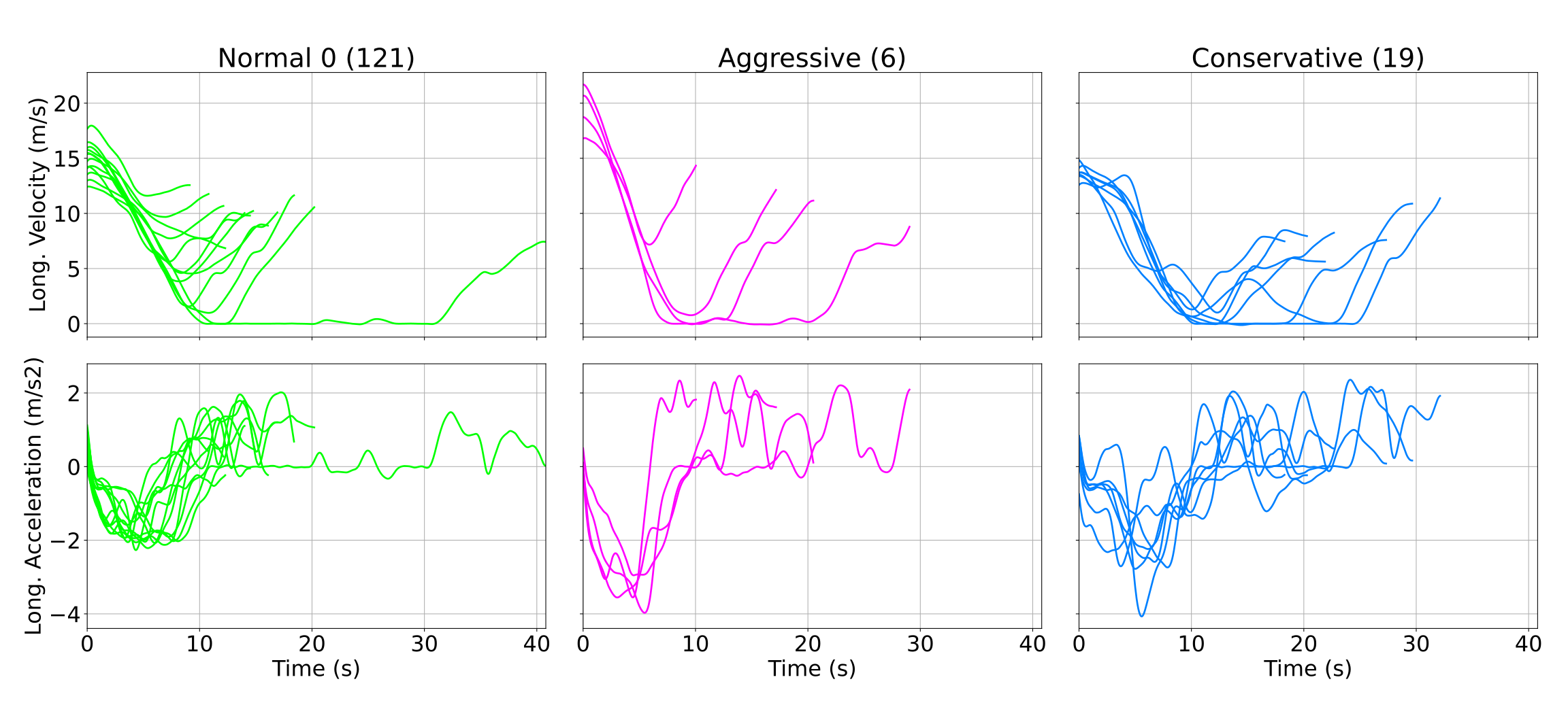
Figure 12: Assertiveness profiles for turn left

To obtain the interaction clusters in Figure 11(b), two features were used, in the same operation: a velocity reduction factor, the minimal velocity from each sample divided by its velocity, and the time below 1 $m/s$. The approach taken here to detect and catalog different interaction profiles concentrated itself on the ego-vehicle, without trying to explain every behavior, providing a wide range of possibilities. In Figure 11 there are multiple instances of interactions, from profiles 4, 3, 7 that reduce their speed to 2, 0, 1 that stopped completely during different times. This approach to obtain all modes of interaction for maneuvers is similar to [31], discovering from data instead of from hand-crafted method as in [32].

IV-E About initialization and convergence

Throughout the procedure, two main points need to be commented: $t_{\text{KL}}$ for each maneuver and the clustering convergence to a local minimum. Since the KL divergence comparison proposed in section III was done using the entire predicted state, i.e. equation (2) and that each trajectory has a range of possible lanes to use, it does make sense to use different values of $t_{\text{KL}}$ per maneuver. A simple exploration process was executed to discover the right interval for this constant. For the turn right it was 4 (Figure 2), given the spread of possible positions at the trajectories’ end, 3 for the turn left and 3.5 for the straight.

Another important point in the clustering procedure is the method’s convergence. According to the algorithm in Figure 5 the final result is obtained only after passing through the merge and split tests without any change in classification. The EM algorithm is guaranteed to converge, but not the split / merge transformation; sometimes the process also ends up in a loop, at which point the result is considered as final. However, given the procedure, only an asymptotic convergence to a local minimal can be assured. And even so, with the samples number increase comes a quadratic computational cost. For example, to cluster the turn right maneuver it took on average $2447.53\pm 949.59$ seconds with $199$ trajectories, while for the straight maneuver it took $28999.2\pm 8982.91$ seconds for 534 trajectories. During the first iterations, the optimized variables $\mu_{nll}$ and $\sigma_{nll}$ decrease rapidly; afterwards the method keeps jumping from different $n_{k}$ values and obtaining only marginal gains. It could be beneficial to set a maximum number of iterations to stop the procedure before this variation. To mitigate this increase in complexity, during the centroid search in Figure 5 only the 30% closest elements are checked if the cluster has more than 100 samples.

Finally, across the four initialization methods tested, there is no clear preference. The same procedure needs to be repeated with different $n_{k}^{i}$ values to obtain an optimal result, given that convergence to a global minimum, where the final values for $\mu_{nll}$, $\sigma_{nll}$ and $n_{k}$ would be always the same, was not observed in our tests. Even the metric being optimized, the sum $\mu_{ll}$ + $\sigma_{ll}$, is not ideal, since it is influenced by the increase on the number of clusters. The merge operation can counterbalance this effect, but it would be better to define a metric that also incorporates the number of clusters.

V CONCLUSIONS

The method proposed here uses the vehicles’ dynamic characteristics to cluster multiple observations into different longitudinal behaviors, together with a probabilistic approach to determine the number of categories that exist. An implementation based on EKF and Mahalanobis distance for the clustering and the KL divergence for the determination on the number of clusters produced for three different maneuvers the distinct longitudinal behaviors expected. However, one drawbacks became evident from the obtained results: the convergence is dependent on $t_{\text{KL}}$, which is itself unique for each maneuver and not easily obtained.

Next steps involve using the obtained clusters to improve the prediction quality of some existent algorithm. Also, these longitudinal clusters will be used to train models for interactive independent agents, creating viable simulations for AV decision making evaluation.

References

- [1] M. Bahari, I. Nejjar, and A. Alahi, “Injecting knowledge in data-driven vehicle trajectory predictors,” Transportation Research Part C: Emerging Technologies, vol. 128, p. 103010, 2021. [Online]. Available: https://www.sciencedirect.com/science/article/pii/S0968090X21000425
- [2] Z. Hu, S. Lou, Y. Xing, X. Wang, D. Cao, and C. Lv, “Review and perspectives on driver digital twin and its enabling technologies for intelligent vehicles,” IEEE Transactions on Intelligent Vehicles, vol. 7, no. 3, pp. 417–440, 2022.
- [3] M. Kuderer, S. Gulati, and W. Burgard, “Learning driving styles for autonomous vehicles from demonstration,” in 2015 IEEE International Conference on Robotics and Automation (ICRA), 2015, pp. 2641–2646.
- [4] Y. Chai, B. Sapp, M. Bansal, and D. Anguelov, “Multipath: Multiple probabilistic anchor trajectory hypotheses for behavior prediction,” 2019. [Online]. Available: https://arxiv.org/abs/1910.05449
- [5] Y. Yanagisawa and T. Satoh, “Clustering multidimensional trajectories based on shape and velocity,” in 22nd International Conference on Data Engineering Workshops (ICDEW’06), 2006, pp. 12–12.
- [6] M. Kerper, C. Wewetzer, H. Trompeter, W. Kiess, and M. Mauve, “Driving more efficiently - the use of inter-vehicle communication to predict a future velocity profile,” in 2011 IEEE 73rd Vehicular Technology Conference (VTC Spring), 2011, pp. 1–5.
- [7] N. de Moura and F. Nashashibi, “Extraction of vehicle behaviors at intersections,” in 2023 IEEE 26th International Conference on Intelligent Transportation Systems (ITSC), 2023, pp. 1779–1786.
- [8] J.-G. Lee, J. Han, and K.-Y. Whang, “Trajectory clustering: a partition-and-group framework,” in Proceedings of the 2007 ACM SIGMOD International Conference on Management of Data, ser. SIGMOD ’07. New York, NY, USA: Association for Computing Machinery, 2007, p. 593–604. [Online]. Available: https://doi.org/10.1145/1247480.1247546
- [9] G. Yuan, P. Sun, J. Zhao, D. Li, and C. Wang, “A review of moving object trajectory clustering algorithms,” Artificial Intelligence Review, vol. 47, no. 1, pp. 123–144, Jan 2017. [Online]. Available: https://doi.org/10.1007/s10462-016-9477-7
- [10] P. C. Besse, B. Guillouet, J.-M. Loubes, and F. Royer, “Review and perspective for distance-based clustering of vehicle trajectories,” IEEE Transactions on Intelligent Transportation Systems, vol. 17, no. 11, pp. 3306–3317, 2016.
- [11] J. Martinsson, N. Mohammadiha, and A. Schliep, “Clustering vehicle maneuver trajectories using mixtures of hidden markov models,” in 2018 21st International Conference on Intelligent Transportation Systems (ITSC), 2018, pp. 3698–3705.
- [12] D. Yi, J. Su, C. Liu, and W.-H. Chen, “Trajectory clustering aided personalized driver intention prediction for intelligent vehicles,” IEEE Transactions on Industrial Informatics, vol. 15, no. 6, pp. 3693–3702, 2019.
- [13] C. Sung, D. Feldman, and D. Rus, “Trajectory clustering for motion prediction,” in 2012 IEEE/RSJ International Conference on Intelligent Robots and Systems, 2012, pp. 1547–1552.
- [14] N. Deo, A. Rangesh, and M. M. Trivedi, “How would surround vehicles move? a unified framework for maneuver classification and motion prediction,” IEEE Transactions on Intelligent Vehicles, vol. 3, no. 2, pp. 129–140, 2018.
- [15] X. Li, K. Zhao, G. Cong, C. S. Jensen, and W. Wei, “Deep representation learning for trajectory similarity computation,” in 2018 IEEE 34th International Conference on Data Engineering (ICDE), 2018, pp. 617–628.
- [16] Z. Fang, Y. Du, L. Chen, Y. Hu, Y. Gao, and G. Chen, “E2dtc: An end to end deep trajectory clustering framework via self-training,” in 2021 IEEE 37th International Conference on Data Engineering (ICDE), 2021, pp. 696–707.
- [17] I. Sutskever, O. Vinyals, and Q. V. Le, “Sequence to sequence learning with neural networks,” 2014. [Online]. Available: https://arxiv.org/abs/1409.3215
- [18] N. Harmening, M. Biloš, and S. Günnemann, “Deep representation learning and clustering of traffic scenarios,” 2020. [Online]. Available: https://arxiv.org/abs/2007.07740
- [19] O. Shouno, “Deep unsupervised learning of a topological map of vehicle maneuvers for characterizing driving styles,” in 2018 21st International Conference on Intelligent Transportation Systems (ITSC), 2018, pp. 2917–2922.
- [20] J. Bock, R. Krajewski, T. Moers, S. Runde, L. Vater, and L. Eckstein, “The ind dataset: A drone dataset of naturalistic road user trajectories at german intersections,” in 2020 IEEE Intelligent Vehicles Symposium (IV). IEEE, 2020, pp. 1929–1934.
- [21] N. de Moura, A. Gervreau-Mercier, F. Garrido, and F. Nashashibi, “Fast maneuver recovery from aerial observation: trajectory clustering and outliers rejection,” in 2024 IEEE Intelligent Vehicles Symposium (IV), 2024. [Online]. Available: https://inria.hal.science/hal-04497008
- [22] S. Thrun, W. Burgard, and D. Fox, Probabilistic Robotics (Intelligent Robotics and Autonomous Agents). The MIT Press, 2005.
- [23] A. J. Krener, “The convergence of the extended kalman filter,” 2002.
- [24] N. D. Moura Martins Gomes, “Governing Automated Vehicle Behavior,” Theses, Sorbonne Université, Jun. 2021. [Online]. Available: https://theses.hal.science/tel-03709568
- [25] G. M. Hoffmann, C. J. Tomlin, M. Montemerlo, and S. Thrun, “Autonomous automobile trajectory tracking for off-road driving: Controller design, experimental validation and racing,” in 2007 American Control Conference, 2007, pp. 2296–2301.
- [26] N. Hashemi and J. Ruths, “Generalized chi-squared detector for lti systems with non-gaussian noise,” in 2019 American Control Conference (ACC), 2019, pp. 404–410.
- [27] S. A. Rodríguez F, V. Frémont, P. Bonnifait, and V. Cherfaoui, “Visual confirmation of mobile objects tracked by a multi-layer lidar,” in 13th International IEEE Conference on Intelligent Transportation Systems, 2010, pp. 849–854.
- [28] G. Chang, “Robust kalman filtering based on mahalanobis distance as outlier judging criterion,” Journal of Geodesy, vol. 88, no. 4, pp. 391–401, Apr 2014. [Online]. Available: https://doi.org/10.1007/s00190-013-0690-8
- [29] G. J. McLachlan and T. Krishnan, The EM algorithm and extensions. John Wiley & Sons, 2007.
- [30] E. F. Saraiva, C. Pereira, and A. K. Suzuki, “A data-driven selection of the number of clusters in the dirichlet allocation model via bayesian mixture modelling,” Journal of Statistical Computation and Simulation, vol. 89, no. 15, pp. 2848–2870, 2019. [Online]. Available: https://doi.org/10.1080/00949655.2019.1643345
- [31] S. Samavi, F. Shkurti, and A. P. Schoellig, “Does unpredictability influence driving behavior?” in 2023 IEEE/RSJ International Conference on Intelligent Robots and Systems (IROS), 2023, pp. 1720–1727.
- [32] T. Gindele, S. Brechtel, and R. Dillmann, “A probabilistic model for estimating driver behaviors and vehicle trajectories in traffic environments,” in 13th International IEEE Conference on Intelligent Transportation Systems, 2010, pp. 1625–1631.