Twist-2 distribution amplitudes of $a_{0}(980)$ and $a_{0}(1450)$

Abstract

Based on QCD sum rules, we investigate the twist-2 distribution amplitudes of the scalar mesons $a_{0}(980)$ and $a_{0}(1450)$. We have derived the moments for these scalar mesons, composed of two constituent valence quarks, to the first order by selecting appropriate correlation functions. Subsequently, we have determined the first two Gegenbauer coefficients of these scalar mesons, employing these moments, we further analyze the twist-2 light-cone distribution amplitudes for the $a_{0}$ meson. The paper concludes with an examination of the weak decay widths for the transitions $B,D\rightarrow a_{0}$.

I Introduction

In the early 1990s, two scalar mesons with properties that challenged the quark model were discovered ${\color[rgb]{0,0,1}[1,2]}$: the mass-degenerate and relatively narrow resonances $f_{0}(980)$ and $a_{0}(980)$. Cribov and colleagues proposed that these could be novel mesons, suggesting their quark-antiquark configurations to be $\frac{u\bar{u}+d\bar{d}}{\sqrt{2}}$ for the isoscalar $f_{0}(980)$ and $\frac{u\bar{u}-d\bar{d}}{\sqrt{2}}$ for the isovector $a_{0}(980)$. Meanwhile, the scalar-meson mass and width patterns led R. L. Jaffe to propose tetraquark assignments for a complete light scalar nonet, potentially explaining the mass degeneracy of $f_{0}(980)$ and $a_{0}(980)$ due to identical four-quark compositions. Despite these scalar mesons—$f_{0}(600)$, $f_{0}(500)$, $K_{0}^{*}(700)$, $f_{0}(980)$ and $a_{0}(980)$—forming a complete light nonet in the current Particle Data Group (PDG) listings, there remains a diversity of perspectives on the $a_{0}(980)$ ${\color[rgb]{0,0,1}[3]}$.

Furthermore, over the past two decades, both theoretical and experimental physicists have achieved significant advancements in the study of $a_{0}(980)$ and $a_{0}(1450)$ ${\color[rgb]{0,0,1}[3-12]}$. Presently, a variety of methods are employed to investigate these particles, including perturbative QCD approaches, QCD sum rules, light-cone sum rules, and phenomenological methods, focusing on aspects such as distribution amplitudes and form factors.

In this paper, we examine the twist-2 distribution amplitudes of the light mesons $a_{0}(980)$ and $a_{0}(1450)$ using the QCD sum rule method. We have calculated the first two non-zero moments of the these two mesons. Additionally, we present the transition form factors for $B,D\rightarrow a_{0}(980),a_{0}(1450)$ decay.

This paper is organised as follow: In Sec. II we derive the general sum rules of moments for twist-2 distribution amplitudes of scalar mesons. In Sec. III we will give the input paraments and the numerical results of the first moments for $a_{0}(980)$ and $a_{0}(1450)$. At the time, the form factors of $B,D\rightarrow a_{0}$ will be obtained. The Sec. IV is devoted to our conclusions.

II QCD sum rule analyses

II.1 Twist-2 distribution amplitudes of scalar mesons

Within the valence quark model, the twist-2 light-cone distribution amplitude $\phi_{s}(x,\mu)$ of scalar mesons $a_{0}$ in the two-quark picture is characterized by the following definition ${\color[rgb]{0,0,1}[13-20]}$

$$\langle S(p)|\bar{q}_{2}(z_{2})\gamma_{\mu}q_{1}(z)|0\rangle=p_{\mu}\int^{1}_{0}dxe^{i(xpz_{2}+\bar{x}pz_{1})}\phi_{s}(x,\mu),$$ (1)

where $x$ represents the momentum fraction of the quark $q_{2}$ within the scalar meson, with $\bar{x}=1-x$. The distribution amplitude $\phi_{s}(x,\mu)$ is subject to the normalization condition

$$\int^{1}_{0}dx\phi_{s}(x,\mu)=f_{s}.$$ (2)

For a light scalar meson, depicted within a two-parton framework, it is capable of coupling to both vector and scalar quark current operators. Consequently, the decay constants can be defined as

$\langle S(p)|\bar{q}_{2}\gamma_{\mu}q_{1}|0\rangle=f_{s}p_{\mu}$,

$\langle S(p)|\bar{q}_{2}q_{1}|0\rangle=m_{s}\bar{f_{s}}$ ,

For charged mesons, the decay constants $f_{s}$ and $\bar{f}_{s}$ are related through the equation of motion

$\mu_{s}f_{s}=\bar{f}_{s}$,

$\mu_{s}=\frac{m_{s}}{m_{2}(\mu)-m_{1}(\mu)}$,

where $m_{1}$, $m_{2}$ and $m_{s}$ denote the masses of $q_{1}$, $q_{2}$ and $a_{0}$, respectively.

Based on the conformal symmetry hidden in the QCD Lagrangin, $\phi_{s}(x,\mu)$ can be expanded in a series of Gengenbauer polynomial $C_{m}^{3/2}$ with increasing conformal spin as

$$\phi_{s}(x,\mu)=\bar{f_{s}}6x(1-x)[1+\mu_{s}\sum_{m=1}^{\infty}B_{m}(\mu)C_{m}^{\frac{3}{2}}(2x-1)].$$ (3)

Here, $C_{m}^{\frac{3}{2}}$ represents the Gegenbaure polynomials.

Utilizing the background field method within QCD, we can compute the moment of the twist-2 distribution amplitude defined in Equation (1). From Equation (1), it is straightforward to deduce

$$\langle 0|\bar{q}_{2}\not{z}(iz\cdot\mathop{D}\limits^{\leftrightarrow}q_{1})^{n}|S(p)\rangle=(z\cdot p)^{n+1}\bar{f}_{s}\langle\xi^{n}\rangle,$$ (4)

with

$$\langle\xi^{n}\rangle=\int_{0}^{1}dx(2x-1)^{n}\phi_{s}(x,\mu).$$ (5)

To calculate the above $\langle\xi^{n}\rangle$ , we consider the following correlation function

$$\Pi_{n}(z,q) =(z\cdot q)^{n+1}I_{n}(q^{2})$$ (6)

$$=i\int d^{4}(x)e^{iqx}\langle 0|T\{O_{n}(x)O^{+}(0)\}|0\rangle,$$

with

$$O_{n}=\bar{q}_{2}\not{z}(iz\cdot\mathop{D}\limits^{\leftrightarrow})^{n}q_{1};\\ O=\bar{q}_{2}q_{1}.$$ (7)

In the deep Euclidean region, the correlation function is calculated using the operator product expansion (OPE), expanded to dimension-6, and presented as

$$I_{n}(q^{2}) =\frac{3}{8\pi^{2}}[5+3\times(-1)^{n}+2n]\frac{1}{(n+1)(n+2)}\ln{\frac{-q^{2}}{\mu^{2}}}[(-1)^{n+1}m_{1}+m_{2}]$$ (8)

$$-\frac{2n+1}{(2n+2)q^{2}}[\langle 0|\bar{q}_{2}q_{2}|0\rangle+(-1)^{n+1}\langle 0|\bar{q}_{1}q_{1}|0\rangle]+\frac{2n+1}{4q^{4}}[m_{2}^{2}\langle 0|\bar{q}_{2}q_{2}|0\rangle+(-1)^{n+1}m_{1}^{2}\langle 0|\bar{q}_{1}q_{1}|0\rangle]$$

$$+\frac{m_{1}m_{2}}{4q^{4}}[\langle 0|\bar{q}_{2}q_{2}|0\rangle+(-1)^{n+1}\langle 0|\bar{q}_{1}q_{1}|0\rangle]-\frac{10+n}{24}\frac{1}{q^{4}}[\langle 0|g\bar{q}_{2}TG\sigma q_{2}|0\rangle+(-1)^{n+1}\langle 0|g\bar{q}_{1}TG\sigma q_{1}|0\rangle]$$

$$-\frac{16(n+1)\pi}{81}\frac{1}{q^{6}}[m_{1}\langle 0|\sqrt{\alpha_{s}}\bar{q}_{2}q_{2}|0\rangle^{2}+(-1)^{n+1}m_{2}\langle 0|\sqrt{\alpha_{s}}\bar{q}_{1}q_{1}|0\rangle^{2}].$$

Conversely, the correlation function may also be evaluated at the hadron level. This involves inserting a complete set of states with quantum numbers matching those of the current operator $O$ into the two-point correlation function. Adopting the definitions

$\langle 0|\bar{q}^{j}_{2}q^{j}_{1}|S(p)\rangle=m_{s}\bar{f}_{s}$,

$\langle 0|\bar{q}^{j}_{1}q^{j}_{2}|S(p)\rangle=0$,

we arrive at the following result for the hadronic representation of the correlation function

$$ImI_{n}^{had}=\pi\delta(s-m_{s}^{2})m_{s}\bar{f}_{s}^{2}\langle\xi^{n}\rangle+\pi\rho^{h}_{s}\theta(s-s_{0}),$$ (9)

where $s_{0}$ is the threshold parameter between ground and excited states. We postulate a density function of the form

$$ImI_{n}^{had}=\pi\delta(s-m_{s}^{2})m_{s}\bar{f}_{s}^{2}\langle\xi^{n}\rangle+\frac{3}{8\pi^{2}}[5+3\times(-1)^{n}+2n]\frac{1}{(n+2)(n+1)}\theta(s-s_{0})$$ (10)

by equating the hadronic and OPE sides, we derive the sum rule

$$I_{n}(q^{2})=\pi\delta(s-m_{s}^{2})m_{s}\bar{f}_{s}^{2}\langle\xi^{n}\rangle+\frac{3}{8\pi^{2}}[5+3\times(-1)^{n}+2n]\frac{1}{(n+2)(n+1)}\theta(s-s_{0}).$$ (11)

Employing the dispersion relation, the correlation function on the hadronic level is matched with the OPE side as follows:

$$\frac{1}{\pi}\int_{0}^{\infty}ds\frac{ImI_{n}(s)}{s-q^{2}}=I^{QCD}_{n}(q^{2}).$$ (12)

To mitigate the impact of higher states—represented by the second term in Equation (12)—we employ the Borel transformation technique, applied uniformly across both sides of the equation. This yields the following expression:

$$\frac{1}{\pi}\frac{1}{M^{2}}\int^{\infty}_{0}dse^{-\frac{s}{M^{2}}}ImI_{n}(s)=B_{M}I^{QCD}_{n}(q^{2}).$$ (13)

where the Borel transform is defined as

$$B_{M}=\lim_{Q^{2},n\rightarrow\inf,\frac{Q^{2}}{n}=M^{2}}\frac{1}{(n-1)!}(Q^{2})^{n}(-\frac{d}{dQ^{2}})^{n}.$$ (14)

Ultimately, the expression for $\langle\xi^{n}\rangle$ is derived as follows

$$\langle\xi^{n}\rangle =\frac{e^{\frac{m^{2}_{s}}{M^{2}}}}{m_{s}\bar{f}^{2}_{s}}\{\frac{3}{16\pi^{2}}[3+(-1)^{n}+2n]\frac{1}{(n+2)(n+1)}[(-1)^{n+1}m_{1}+m_{2}](1+e^{-\frac{s_{0}}{M^{2}}})$$ (15)

$$+\langle 0|\bar{q}_{2}q_{2}|0\rangle+(-1)^{n+1}\langle 0|\bar{q}_{1}q_{1}|0\rangle+\frac{2n+1}{2M^{2}}[m_{2}^{2}\langle 0|\bar{q}_{2}q_{2}|0\rangle+(-1)^{n+1}m_{1}^{2}\langle 0|\bar{q}_{1}q_{1}|0\rangle]$$

$$+\frac{m_{1}m_{2}}{2M^{2}}[\langle 0|\bar{q}_{2}q_{2}|0\rangle+(-1)^{n+1}\langle 0|\bar{q}_{1}q_{1}|0\rangle]-\frac{2n}{3}\frac{1}{M^{2}}[\langle 0|g\bar{q}_{2}TG\sigma q_{2}|0\rangle+(-1)^{n+1}\langle 0|g\bar{q}_{1}TG\sigma q_{1}|0\rangle]$$

$$+\frac{8n\pi}{81}\frac{1}{M^{4}}[m_{1}\langle 0|\sqrt{\alpha_{s}}\bar{q}_{2}q_{2}|0\rangle^{2}+(-1)^{n+1}m_{2}\langle 0|\sqrt{\alpha_{s}}\bar{q}_{1}q_{1}|0\rangle^{2}]\}.$$

For scalar mesons such as the $a_{0}(980)$ and $a_{0}(1450)$, where the quark-antiquark pair is $\bar{u}d$, the aforementioned equation is reformulated as follows

$$\langle\xi^{n}\rangle =\frac{e^{\frac{m^{2}_{s}}{M^{2}}}}{m_{s}\bar{f}^{2}_{s}}\{\frac{3}{16\pi^{2}}[3+(-1)^{n}+2n]\frac{1}{(n+2)(n+1)}[(-1)^{n+1}m_{u}+m_{d}](1+e^{-\frac{s_{0}}{M^{2}}})$$ (16)

$$+\langle 0|\bar{d}d|0\rangle+(-1)^{n+1}\langle 0|\bar{u}u|0\rangle+\frac{2n+1}{2M^{2}}[m_{2}^{2}\langle 0|\bar{d}d|0\rangle+(-1)^{n+1}m_{1}^{2}\langle 0|\bar{u}u|0\rangle]$$

$$+\frac{m_{1}m_{2}}{2M^{2}}[\langle 0|\bar{d}d|0\rangle+(-1)^{n+1}\langle 0|\bar{u}u|0\rangle]-\frac{2n}{3}\frac{1}{M^{2}}[\langle 0|g\bar{d}TG\sigma d|0\rangle+(-1)^{n+1}\langle 0|g\bar{u}TG\sigma u|0\rangle]$$

$$+\frac{8n\pi}{81}\frac{1}{M^{4}}[m_{u}\langle 0|\sqrt{\alpha_{s}}\bar{d}d|0\rangle^{2}+(-1)^{n+1}m_{d}\langle 0|\sqrt{\alpha_{s}}\bar{u}u|0\rangle^{2}]\}.$$

For even values of $n$ , the expression for the even moments is given by

$$\langle\xi^{n}\rangle =\frac{e^{\frac{m^{2}_{s}}{M^{2}}}}{m_{s}\bar{f}^{2}_{s}}\{\frac{3}{16\pi^{2}}[3+4n]\frac{1}{(n+2)(n+1)}[-m_{u}+m_{d}](1+e^{-\frac{s_{0}}{M^{2}}})$$ (17)

$$+\langle 0|\bar{d}d|0\rangle-\langle 0|\bar{u}u|0\rangle+\frac{2n+1}{2M^{2}}[m_{2}^{2}\langle 0|\bar{d}d|0\rangle-m_{1}^{2}\langle 0|\bar{u}u|0\rangle]$$

$$+\frac{m_{1}m_{2}}{2M^{2}}[\langle 0|\bar{d}d|0\rangle-\langle 0|\bar{u}u|0\rangle]-\frac{2n}{3}\frac{1}{M^{2}}[\langle 0|g\bar{d}TG\sigma d|0\rangle-\langle 0|g\bar{u}TG\sigma u|0\rangle]$$

$$+\frac{8n\pi}{81}\frac{1}{M^{4}}[m_{u}\langle 0|\sqrt{\alpha_{s}}\bar{d}d|0\rangle^{2}-m_{d}\langle 0|\sqrt{\alpha_{s}}\bar{u}u|0\rangle^{2}]\}.$$

The analysis of the equation reveals that the contribution from $\langle\xi^{n}\rangle$ is minimal for even values of $n$. Consequently, our focus shifts to the non-vanishing odd moments, specifically $\langle\xi^{1}\rangle$ and $\langle\xi^{3}\rangle$, which are given by

$$\langle\xi^{1}\rangle =\frac{e^{\frac{m^{2}_{s}}{M^{2}}}}{m_{s}\bar{f}^{2}_{s}}\{-\frac{1}{8\pi}[m_{u}+m_{d}](1+e^{-\frac{s_{0}}{M^{2}}})$$ (18)

$$+\langle 0|\bar{d}d|0\rangle+\langle 0|\bar{u}u|0\rangle+\frac{3}{2M^{2}}[m_{2}^{2}\langle 0|\bar{d}d|0\rangle+m_{1}^{2}\langle 0|\bar{u}u|0\rangle]$$

$$+\frac{m_{1}m_{2}}{2M^{2}}[\langle 0|\bar{d}d|0\rangle+\langle 0|\bar{u}u|0\rangle]-\frac{2}{3}\frac{1}{M^{2}}[\langle 0|g\bar{d}TG\sigma d|0\rangle+\langle 0|g\bar{u}TG\sigma u|0\rangle]$$

$$+\frac{8\pi}{81}\frac{1}{M^{4}}[m_{u}\langle 0|\sqrt{\alpha_{s}}\bar{d}d|0\rangle^{2}+m_{d}\langle 0|\sqrt{\alpha_{s}}\bar{u}u|0\rangle^{2}]\},$$

$$\langle\xi^{3}\rangle =\frac{e^{\frac{m^{2}_{s}}{M^{2}}}}{m_{s}\bar{f}^{2}_{s}}\{-\frac{3}{40\pi}[m_{u}+m_{d}](1+e^{-\frac{s_{0}}{M^{2}}})$$ (19)

$$+\langle 0|\bar{d}d|0\rangle+\langle 0|\bar{u}u|0\rangle+\frac{5}{2M^{2}}[m_{2}^{2}\langle 0|\bar{d}d|0\rangle+m_{1}^{2}\langle 0|\bar{u}u|0\rangle]$$

$$+\frac{m_{1}m_{2}}{2M^{2}}[\langle 0|\bar{d}d|0\rangle+\langle 0|\bar{u}u|0\rangle]-\frac{2}{M^{2}}[\langle 0|g\bar{d}TG\sigma d|0\rangle+\langle 0|g\bar{u}TG\sigma u|0\rangle]$$

$$+\frac{8\pi}{27}\frac{1}{M^{4}}[m_{u}\langle 0|\sqrt{\alpha_{s}}\bar{d}d|0\rangle^{2}+m_{d}\langle 0|\sqrt{\alpha_{s}}\bar{u}u|0\rangle^{2}]\}.$$

It should be noted that all parameters within the aforementioned sum rules are defined at the scale of the Borel parameter $M$. The renormalization group equations for the decay constant, quark mass, and condensate are expressed as follows

$\bar{f}_{s}(M)=\bar{f}_{s}(\mu)(\frac{\alpha_{s}(\mu)}{\alpha_{s}(M)})^{\frac{4}{b}}$,

$m_{q;M}=m_{q;\mu}(\frac{\alpha_{s}(\mu)}{\alpha_{s}(M)})^{\frac{4}{b}}$,

$\langle 0|\bar{q}q|0\rangle_{M}=\langle 0|\bar{q}q|0\rangle_{\mu}(\frac{\alpha_{s}(\mu)}{\alpha_{s}(M)})^{\frac{4}{b}}$,

$\langle 0|g\bar{q}TG\sigma q|0\rangle_{M}=\langle 0|g\bar{q}TG\sigma q|0\rangle_{\mu}(\frac{\alpha_{s}(\mu)}{\alpha_{s}(M)})^{\frac{4}{b}}$,

$\langle 0|\sqrt{\alpha_{s}}\bar{q}q|0\rangle^{2}_{M}=\langle 0|\alpha_{s}\bar{q}q|0\rangle^{2}_{\mu}(\frac{\alpha_{s}(\mu)}{\alpha_{s}(M)})^{\frac{4}{b}}$.

Here, $b=\frac{33-2n_{f}}{3}$ and $n_{f}$ and $n_{f}$ represents the number of quark flavors. Additionally, the orthogonality relation for the Gegenbauer polynomials is given by

$$\int^{1}_{0}dxx(1-x)C^{\frac{3}{2}}_{m}(2x-1)C^{\frac{3}{2}}_{n}(2x-1)=\frac{(n+1)(n+2)}{4(2n+3)}\delta_{mn}.$$ (20)

Considering Eq.(3), we can obtain the relation between Gegenbauer coefficients and $\langle\xi^{n}\rangle$

$$B_{1}=\frac{5}{3}\langle\xi^{1}\rangle,$$ (21)

$$B_{3}=\frac{21}{4}\langle\xi^{3}\rangle-\frac{9}{4}\langle\xi^{1}\rangle.$$

The renormalization group equations governing the Gegenbauer moments are articulated as

$$B_{n}(\mu)=B_{n}(\mu_{0})(\frac{\alpha_{s}(\mu_{0})}{\alpha_{s}(M)})^{-\frac{\gamma_{n}-4}{b}},$$ (22)

where the anomalous dimension $\gamma_{n}$ is

$$\gamma_{n}=C_{f}(1-\frac{2}{(n+1)(n+2)})+\sum_{j=2}^{n+1}\frac{1}{j}.$$ (23)

The constant $C_{f}$ is assigned the value of $\frac{4}{3}$, which is pivotal in our subsequent calculations.

II.2 $B/D\rightarrow S$ form factors with the light-cone sum rules

To elucidate the form factors, we construct the two-point correlation function as follows ${\color[rgb]{0,0,1}[21-25]}$

$$\Pi_{1\mu}(p,q)=i\int d^{4}xe^{iqx}\langle S(p)|T\{\bar{q}_{2}(x)\gamma_{\mu}(1+\gamma_{5})Q(x),\bar{Q}(0)i(1+\gamma_{5})q_{1}(0)\}|0\rangle,\\$$ (24)

where $S$ denotes the light scalar mesons, and $Q$ represents either $b$ or $c$ quark. The momentum transfer $q$ is defined as $q=p_{M}-p$, with $p_{M}$ and $p$ being the four-momenta of the initial $B/D$ mesons and final scalar meson $s(P)$, respectively.

Typically, the correlation function is delineated employing two distinct methodologies: 1) the hadronic characteristics, alluding to the phenomenological aspect, and 2) the quark and gluon degrees of freedom, representing the theoretical facet. By aligning these two perspectives and invoking the Borel transformation to mitigate the influence of higher states and the continuum, we derive the sum rule expressions for the form factors.

On the phenomenological front, singling out the mass term of the pseudoscalar $D$ meson yields

$$\Pi_{1\mu}(p,q)=\frac{\langle S(p)|\bar{q}_{2}\gamma_{\mu}\gamma_{5}c|M\rangle\langle M|\bar{c}i\gamma_{5}q_{1}|0\rangle}{m^{2}_{D}-(p+q)^{2}}+higher\quad states,\\$$ (25)

where the pseudoscalar meson $B/D$ is represented as $|M\rangle$ and the form factors are articulated through the matrix elements

$$\langle S(p)|\bar{q}_{2}\gamma_{\mu}\gamma_{5}Q|M\rangle=-2if_{+}^{S}(q^{2})p_{\mu}-i[f_{+}^{S}(q^{2}+f_{-}^{S}(q^{2}))]q_{\mu},$$ (26)

with $f_{+}^{S}$ and $f_{-}^{S}$ being the transition form factors for $B/D\rightarrow S$, $m_{M}$, $m_{S}$, $m_{Q}$ and $m_{q_{1}}$representing the masses of the $B/D$ meson, scalar meson, heavy quark $Q$, and light quark, respectively. Subsequently, the phenomenological side is expressed as

$$\Pi_{1\mu}(p,q)=-\frac{2f_{+}(q^{2})p_{\mu}+[f_{+}(q^{2})+f_{-}(q^{2})]q_{\mu}}{m_{M}^{2}-(p+q)^{2}}\frac{m^{2}_{B/D}f_{M}}{m_{Q}+m_{q_{1}}}+\int_{s_{0}}^{\infty}\frac{\rho(s)ds}{s-(p+q)^{2}},\\$$ (27)

where $f_{M}$ is the decay constant of $B/D$ meson, $\rho(s)$ is the spectral density of the higher states and continuum, and $s_{0}$ is the threshold parameter between the ground and excited states.

On the theoretical side, the computation of the correlation function in the domain of large spacelike momentum is predicated on the expansion of the time-ordered product T near the light cone.

With the propagator of the heavy quark $Q$, formulated as

$$S(x)=-i\int\frac{d^{4}k}{(2\pi)^{4}}e^{-ik\cdot x}\frac{\not{k}+m_{Q}}{m^{2}_{Q}-k^{2}},$$ (28)

and the lgingt-cone distribution amplitude (1), the correlation function on the theoretical side is expressed as

$$\Pi_{1\mu}=2im_{Q}p_{\mu}\int^{1}_{0}dx\frac{\phi_{S}(x,\mu)}{m^{2}_{Q}-(q+up)^{2}},\\$$ (29)

By equating the coefficients of the corresponding Lorentz structures on the phenomenological side with those on the theoretical side and applying the Borel transformation to both, we acquire the sum rules for the form factors

$$f_{+}(q^{2}) =-\frac{m_{Q}+m_{q_{1}}}{m_{M}^{2}f_{M}}m_{Q}\int^{1}_{\Delta}\frac{\phi(x)}{x}dxe^{FF},$$ (30)

$$f_{-}(q^{2}) =\frac{m_{Q}+m_{q_{1}}}{m_{B/D}^{2}f_{B/D}}m_{Q}\int^{1}_{\Delta}\frac{\phi(x)}{x}dxe^{FF},$$

where the function $FF$ is given by

$$FF =-\frac{1}{xM^{2}}(m^{2}_{Q}+u\bar{x}p^{2}-\bar{x}q^{2})+\frac{m^{2}_{M}}{M^{2}},$$ (31)

and $\Delta$ is defined as

$$\Delta =\frac{\sqrt{(s_{0}-m_{S}^{2}-q^{2})^{2}+4(m_{Q}^{2}-q^{2})m_{S}^{2}}\--(s_{0}-m_{S}^{2}-q^{2})}{2m_{S}^{2}}.$$ (32)

III Numerical analyses and discussion

The input parameters involved in the numerical calculation are as follows

$m_{u}=2.16\ \rm{MeV}$

$m_{d}=4.67\ \rm{MeV}$

$m_{a_{0}(980)}=0.98\ \rm{GeV}$

$m_{a_{0}(1450)}=1.474\ \rm{GeV}$

$\langle u\bar{u}\rangle=\langle d\bar{d}\rangle=-0.24^{3}\rm{GeV^{3}}$

$\langle g_{s}\bar{u}\sigma Gu\rangle=\langle g_{s}\bar{d}\sigma Gd\rangle=0.8\times\langle u\bar{u}\rangle=0.8\times\langle d\bar{d}\rangle$

$m_{0}^{2}=0.8\ \rm{GeV^{2}}$

$\alpha_{s}=0.517$

For the $a_{0}(980)$ parameters, the scale is set at $\mu=1\ \rm{GeV}$, and for the $a_{0}(1450)$ parameters, the scale is $\mu=2\ \rm{GeV}$. The Borel parameter and threshold are chosen to be within ranges that adhere to the conventional constraints of sum rule calculations. To delineate the Borel window for $M^{2}$, we present an analysis of the Borel parameter curves and their slopes for the moments in Figures 1 and 2. (Figures 1 and 2 would be included here to illustrate the analysis.)

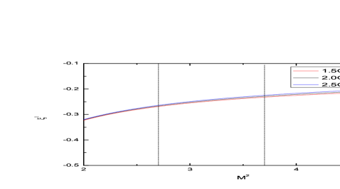
(a) $\xi^{1}$

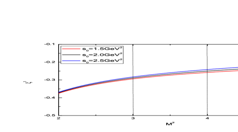
(b) $\xi^{3}$

Figure 1: The first moment (left panel)$\xi^{1}$ and the third moment (right panel) $\xi^{3}$ of the $a_{0}(980)$.

Subsequently, we have identified the Borel windows for the first moment of the $a_{0}(980)$ meson as the interval $[2.7,3.7]\ \rm{GeV^{2}}$, and for the third moment as $[3,4]\ \rm{GeV^{2}}$, as illustrated in Figure 1. It is evident that the dependence of the moments on $M^{2}$ is minimal, indicating that the calculated moments exhibit substantial stability. Additionally, the moments’ reliance on the threshold parameter is found to be nominal. The criterion for selecting the appropriate Borel window is based on the condition that the slope of the curves $\xi^{\prime}(M^{2})$ does not exceed $5\%$.

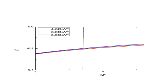
(a) $\xi^{1}$

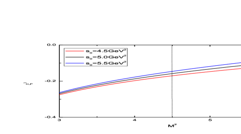
(b) $\xi^{3}$

Figure 2: The first moment (left panel)$\xi^{1}$ and the third moment (right panel) $\xi^{3}$ of the $a_{0}(1450)$.

In an analogous manner, the Borel windows for the initial two moments of the $a_{0}(1450)$ meson have been determined and are presented in Figure 2. The first moment’s Borel window is identified within the range of $[3.7,4.7]\rm{GeV^{2}}$, while the third moment falls between $[4.5,5.5]\rm{GeV^{2}}$. It is also observed that the influence of the threshold parameter on the outcomes derived from the QCD sum rule analysis is marginal.

Additionally, for the $a_{0}(980)$ meson, the moments are calculated with specific values of $M^{2}$ and $s_{0}$. At $M^{2}=3.2\rm{GeV^{2}}$ for $\xi^{1}$ and $M^{2}=3.5\rm{GeV^{2}}$ for $\xi^{3}$, with $s_{0}=2.0\rm{GeV^{2}}$, we find $\xi^{1}=-0.25$, and $\xi^{3}=-0.27$. Employing a parallel approach for the $a_{0}(1450)$ meson, the moments are determined at $M^{2}=4.2\rm{GeV^{2}}$ for $\xi^{1}$ and $M^{2}=5.0\rm{GeV^{2}}$ for $\xi^{3}$, given $s_{0}=5.0\rm{GeV^{2}}$, yielding $\xi^{1}=-0.18$ and $\xi^{3}=-0.13$. Subsequently, the twist-2 distribution amplitudes $\phi$ are derived and depicted in Figure 3.

(a) $a_{0}(980)$

(b) $a_{0}(1450)$

Figure 3: The distribution amplitudes of $a_{0}(980)$ (left panel) and $a_{0}(1450)$ (right panel).

As illustrated in Figure 3, the threshold parameter exerts minimal influence on the $a_{0}(980)$ meson; in contrast, the $a_{0}(1450)$) meson is more significantly influenced by the threshold. Utilizing the determined values of the Gegenbauer coefficients, $B_{1}=-0.718$ and $B_{3}=-0.011$ for the $a_{0}(980)$, and $B_{1}=-0.3$ and $B_{3}=-0.23$ for the $a_{0}(1450)$, we have calculated the form factors for the transitions $B\rightarrow a_{0}(980)$, $B\rightarrow a_{0}(1450)$, $D\rightarrow a_{0}(980)$, and $D\rightarrow a_{0}(1450)$. The results are presented in Table 1, alongside values from other studies for comparative analysis.

Process	$B\rightarrow a_{0}(980)$		$B\rightarrow a_{0}(1450)$		$D\rightarrow a_{0}(980)$		$D\rightarrow a_{0}(1450)$
Form factor	$f_{+}$	$f_{-}$	$f_{+}$	$f_{-}$	$f_{+}$	$f_{-}$	$f_{+}$	$f_{-}$
Our work	0.66	-0.66	0.23	-0.23	0.53	-0.53	0.28	-0.28
S1	0.56	-0.56	0.26	-0.26
S2			0.53	-0.53
LS			0.52	-0.44
pS1	0.39		-0.31
pS2			0.68
LCSR1					0.85	-0.85	0.94	-0.94
LCSR2					1.75	0.31
CCQM					0.55
CLFQM							0.51

IV Summary

In the present study, we have conducted an in-depth analysis of the twist-2 distribution amplitudes for the $a_{0}(980)$ and $a_{0}(1450)$ mesons, grounded in the framework of Quantum Chromodynamics (QCD) sum rules. Concurrently, we performed calculations for the form factors associated with the transitions $D\rightarrow a_{0}(980)$, and $D\rightarrow a_{0}(1450)$. These calculations served to verify the accuracy of the moments obtained in our analysis.

Our findings contribute to a deeper understanding of the scalar mesons’ properties and provide valuable insights for further theoretical and experimental investigations in the field of particle physics.