Analysis of a Class of Two-delay Fractional Differential Equation
Abstract
The differential equations involving two discrete delays are helpful in modeling two different processes in one model. We provide the stability and bifurcation analysis in the fractional order delay differential equation in the -plane. Various regions of stability include stable (S), unstable (U), single stable region (SSR), and stability switch (SS). In the stable region, the system is stable for all the delay values. The region SSR has a critical value of delay that bifurcates the stable and unstable behavior. Switching of stable and unstable behaviors is observed in the SS region.
1 Introduction
Differential equation is a popular tool used in the mathematical modeling of physical systems. If the order of derivative in such a model is a non-integer, it is called a fractional differential equation (FDE) [1, 2]. The basic theory of FDEs is developed in [3, 4, 5, 6, 7, 8]. Luchko and Gorenflo [9] developed an operational method to find analytical solutions to the linear FDEs. Generalization of fractional order can be done in many ways. A few popular fractional order derivatives (FOD) are Grunwald-Letnikov, Riemann-Liouville, and Caputo [1]. The fractional derivative operators are nonlocal, unlike the classical derivatives, and hence the properties and results may be complicated [10, 11]. Numerical methods to solve FDEs are also time-consuming. Diethelm et al. [12] developed a predictor-corrector method to solve FDEs. Daftardar-Gejji et al. [13] improved this method and developed a new predictor-corrector method. Approximate analytical solutions of FDEs on a smaller interval are given by Adomian decomposition method [14, 15], new iterative method [16], homotopy perturbation method [17] and so on. In his seminal work [18], Matignon proposed the stability of the fractional order dynamical systems. The results are further explored by Tavazoei and Haeri [19]. Fractional order counterparts of the popular chaotic systems are well studied in the literature [20, 21, 22, 23, 24, 25]. It is observed that the fractional order systems can show chaos for the system dimension less than three, unlike their classical counterparts. Control methods to synchronize chaos are developed by Zhou and Li [26], Deng [27], Bhalekar and Daftardar-Gejji [28], Martínez-Guerra and Pérez-Pinacho [29] among others.
Hilfer discussed fractional calculus (FC) applications in physics in [30]. Mainardi worked on the FC in the viscoelasticity [31]. Magin [32, 33] presented various applications of FC in bioengineering.
The time delay can also be used to model a memory in the system, like a fractional derivative. The delay differential equations (DDE) are the infinite dimensional dynamical systems with rich dynamics [34, 35]. One can have chaos in a single scalar DDE, unlike its nondelayed counterpart [36, 37, 38]. As we can expect the effect of past states on the present and future, the occurrence of the delay is natural. A variety of applications of DDEs are presented in [34, 39, 40, 41, 42, 43]. If one combines an FDE and a DDE, then the resulting fractional-order delay differential equation (FDDE) may lead to an interesting dynamical system. These systems will be advantageous in the view of applications. At the same time, the analysis of such systems will be challenging. The characteristic equations of FDDEs are transcendental equations containing the terms of the form and making them complicated. Bhalekar [44, 45] presented the stability analysis of . The analysis is further explored by Bhalekar and Gupta in [46, 47, 48, 49]. Numerical schemes to solve FDDEs are developed by Bhalekar and Daftardar-Gejji [50] and Daftardar-Gejji et al. [51]. Chaos in FDDEs is studied in [52, 53, 54, 55]. Bhalekar et al. [56] worked on the fractional order bloch equation arising in NMR.
The DDEs
| (1) |
or their linearization at an equilibrium point
| (2) |
involving two delays and are well-studied dynamical systems. Beuter et al. [57, 58] used these equations to model human neurological diseases. Piotrowska [59] mentioned that the two delays model the two cellular processes, viz. proliferation and apoptosis. Belair et al. [60] studied erythropoiesis using these equations. Braddock and Driessche [61] employed them in the population dynamics. The stability of these equations is analyzed by Hale and Hunag [62], Braddock and Driessche [61], Mahaffy, Joiner and Zak [63], Li, Ruan and Wei [64] among others. Nussbaum [65] studied the periodic solutions in these equations.
The above discussion shows the importance of FDDEs and systems of the form (1) and (2). This motivates us to study the fractional order generalizations
| (3) |
and
| (4) |
Bhalekar [66] studied (4) with . In general, it is challenging to analyze these equations. Therefore, we consider a particular case of the equation (4) by setting and . The paper is organized as below:
2 Preliminaries
Definition 2.1.
A real function is said to be in space if there exists a real number such that , where
Definition 2.2.
A real function , is said to be in space , if
Definition 2.3.
Let and , then the Riemann Liouville integral of of order , is given by
Definition 2.4.
The Caputo fractional derivative of , is defined as
Note that for
2.1 Basic result
Theorem 2.1.
[44]
Suppose is an equilibrium solution of the generalized delay differential equation and
-
1.
If then the stability region of in parameter space is located between the plane and
The equation undergoes Hopf bifurcation at this value.
-
2.
If then is unstable for any .
-
3.
If and then is unstable for any .
3 Main Results
Consider the fractional delay differential equation
| (5) |
where is a Caputo fractional derivative of order is the delay. The characteristic equation of this system can be found using the Laplace transform [68] as below
| (6) |
By multiplying the above equation with to get a new equation with a less number of parameters, we get
| (7) |
3.1 Stability Analysis
We conduct the stability analysis using the same approach outlined in [34].
The system is asymptotically stable if all the roots of (6) satisfy
| (8) |
If , then the condition (8) simplifies to the form
which gives using .
Now, we take and discuss the properties of roots of (6). Note that the sign of will be the same as that of . Therefore, we analyze eq. (7) and provide the properties of eq. (6) using the relation .
We write and find the expressions for the curves which are the boundaries of the stable region in the -plane.
On the boundary of the stable region, the condition
| (9) |
hold. If , the boundary condition 9 will become , which gives (by (7)).
So, is a branch of the boundary curve in the -plane. Since for , is the stability region and is the boundary curve, so , i.e., positive -axis is the region of instability. In the following theorem, we prove that for every , the system will be unstable in the first and fourth quadrants of the -plane.
Theorem 3.1.
Whenever , the fractional delay differential equation
is unstable for all .
Proof.
Consider the modified characteristic equation (7).
Take and
We prove that there always exists a positive real root of (7) whenever , i.e., there always exists a s.t , whenever .
We consider two cases:
Case 1: Assume and (i.e first quadrant).
If and then and
It can be easily seen that and .
Since . Therefore, is monotonic increasing. Also, .
Hence, .
Now, and
Also, we observe that when and . Hence, has a local maxima (say ) and
So,
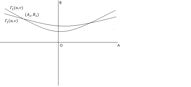
We can conclude that (see Figure 1).
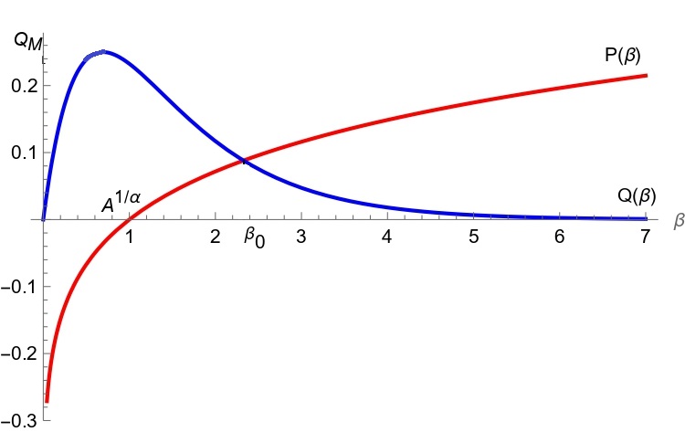
Hence, there always exist some s.t .
This shows that there exists a real positive root to (7). So, the system is unstable in the first quadrant.
Case 2: Assume and (i.e fourth quadrant).
Therefore, we have and
Since the function is independent of ,
the in this case also.
Now, and
Also, we observe that when and Hence, in this case, has a local minima (say ) and
So,
We can conclude that (see Figure 2).
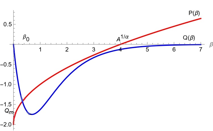
Hence, there always exist some s.t . Note that we can have one, two, or three such intersection points , This shows that a real positive root to (7). So, the system is unstable in the fourth quadrant also.
∎
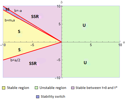
Note: We denote the unstable region in the -plane by the letter ’U’ in Figure 8.
Now, we analyze the stability in the second and third quadrants.
If , then condition (9) gives . Since is also a root of (7), we may take . By putting in and solving for A and B in terms of parameter , the following expressions can be obtained:
| (10) | |||||
| (11) |
In Figure 3, we present the parametric plots of for some values of restricted to second and third quadrants of AB-plane. These restricted subintervals of are given by
Note that, at the left end of each of these subintervals, and at the right end, becomes an unbounded curve. If is very small, there is no intersection between the first and second branches.
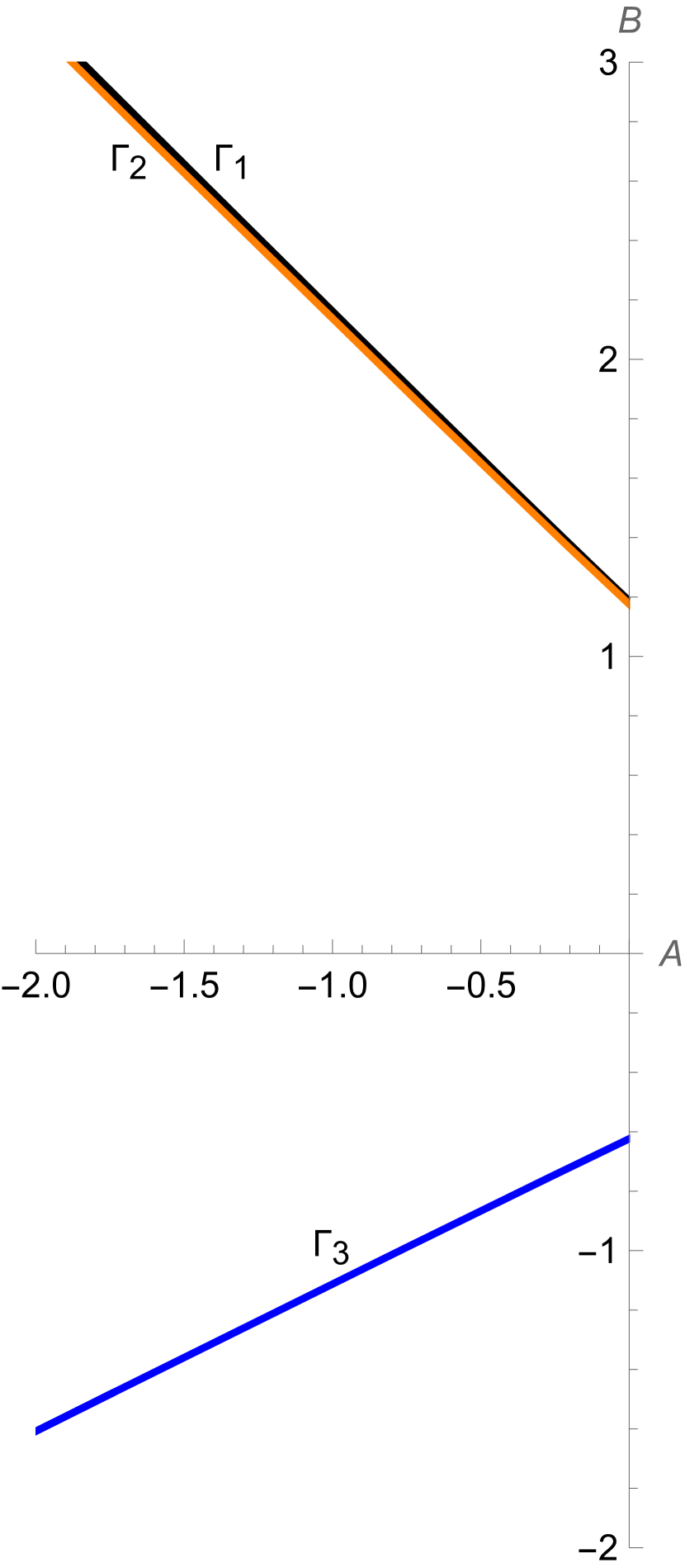
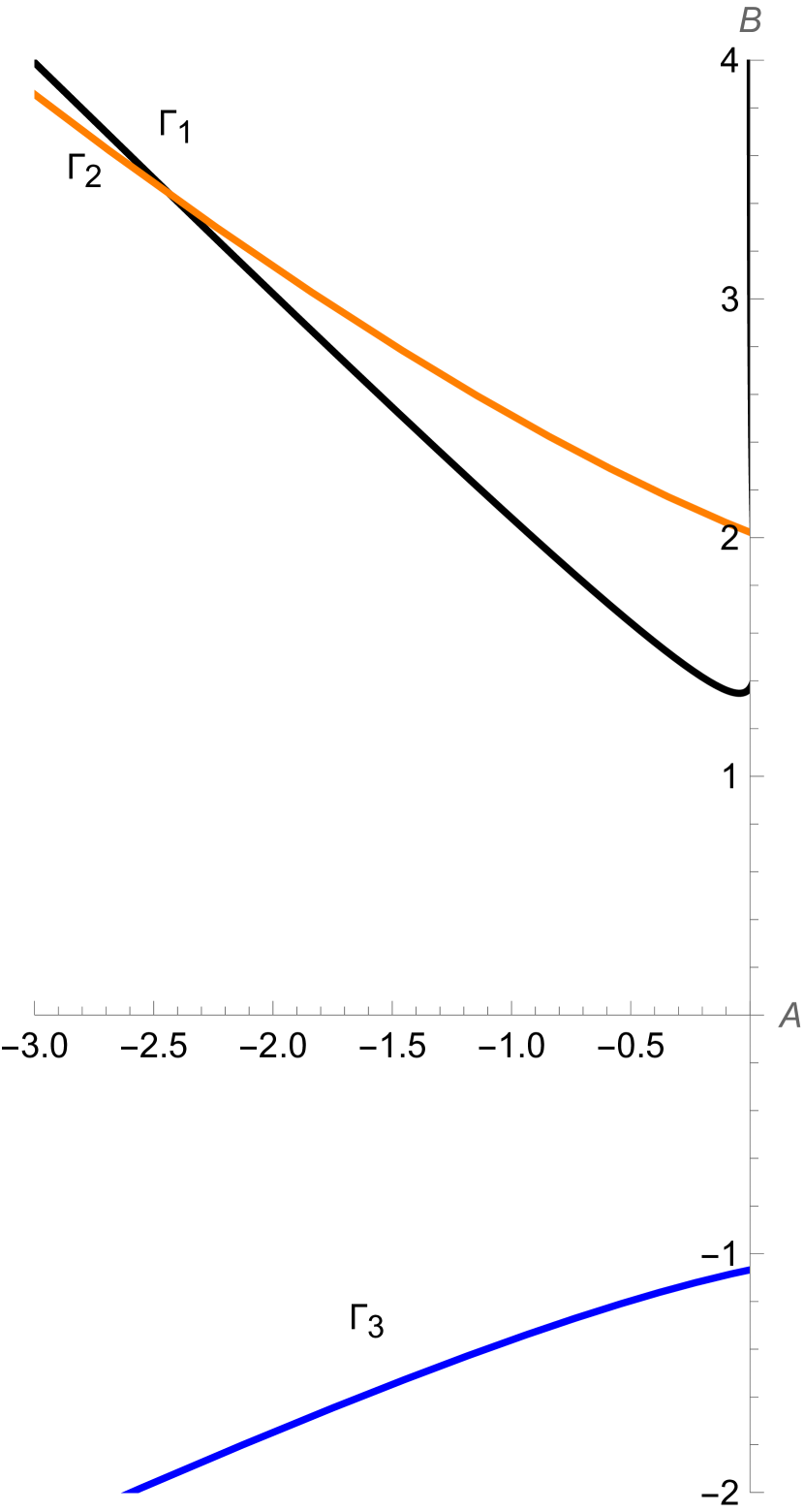
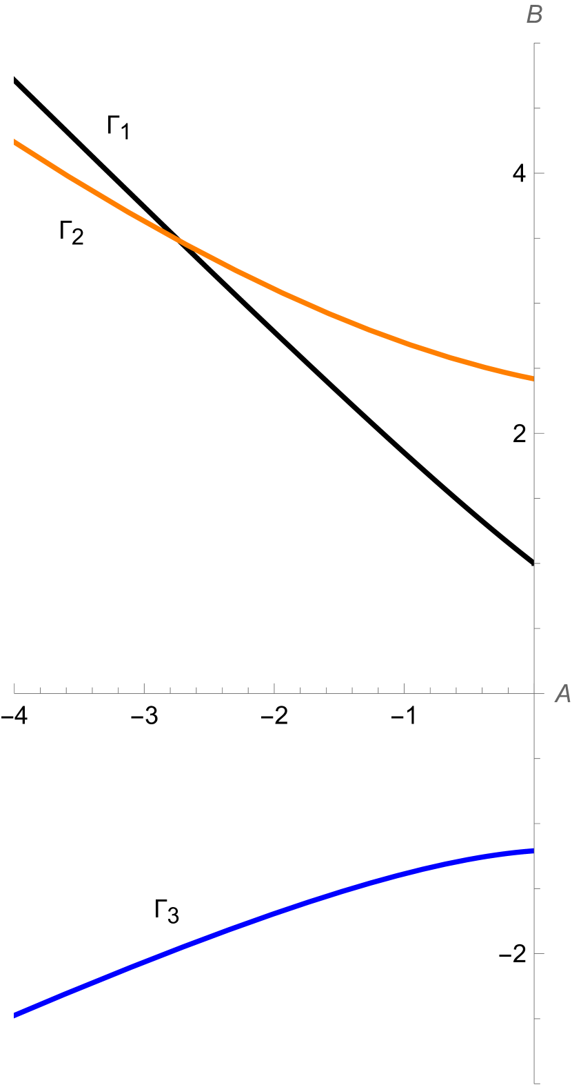
For , the system is stable if , which is the negative A-axis. After this, the stability will change at the branches of curves given in Figure 3.
To get those critical values where the stability will change, we first find the value of corresponding to the critical value of delay. Such values of can be determined by solving
| (12) |
Note that (12) is obtained by using the relations i.e. .
Since this is a transcendental equation, it will have many roots.
By putting different values of and value in the respective quadrants, we get two values of in the second quadrant and one in the third.
Now, in the second quadrant, we have two branches of the curve parametrized by (10) and (11), namely ,
The boundary of the stable region in this quadrant is given by the part of the branch that is closest to the A-axis. We denote the boundary in this quadrant as .
In the third quadrant, there is only one branch of the curve , namely for .
Observations 2.1
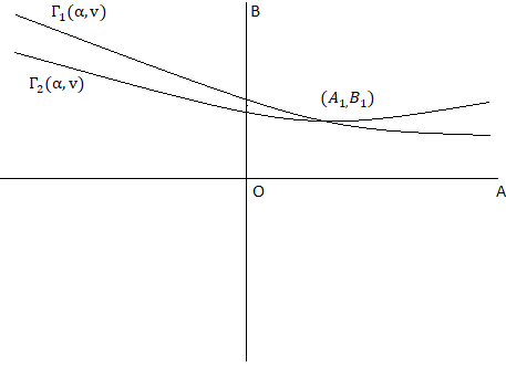
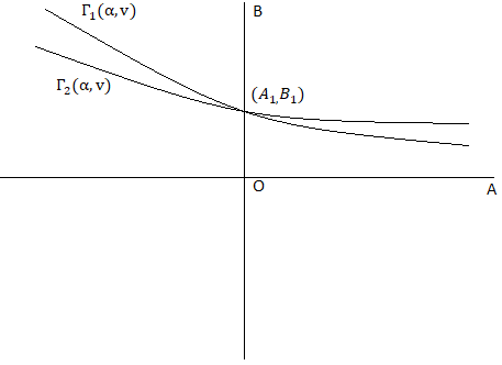
In the second quadrant, bifurcates the two behaviors as follows (see Figure 5):
-
•
If then the second branch is closest to the -axis and hence, it is the boundary of the stable region in the second quadrant (e.g., see Figure 3(a)) i.e.,
-
•
If then the curves and intersect at a point, say (e.g. see Figures 3(b),3(c),3(d)). (see data set 1 for the code to find numerically and Figure 4 for the graph.)
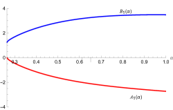
Figure 4: Curves and -
–
If then the boundary is given by ,
-
–
If then gives the boundary.
-
–
i.e.,
| (13) |
At the bifurcation point, the two branches of the boundary curve have an intersection on the B-axis. So, for such that
As already discussed, So,
Therefore, we solve to get the approximate value of the bifurcation point viz.
The stable region is bounded by the curves closest to the negative axis. The region outside the stable region is the unstable one. Thus, Figure 3 show the stable and unstable regions for the modified characteristic equation (7).
Note that the stability in the -plane depends on delay also. In the next section, we discuss such regions in the -plane.
4 Stability diagram in -plane
In this section, we use the analysis in section 3 and provide various stable regions in the -plane for the given DDE (5).
Recall, . For any fixed , we consider the vector
At is at origin in the -plane. As we increase represents an arrow.
We have the following behaviors:
-
1.
For given pair generates an arrow which lies entirely in the unstable region in the -plane. Such pairs form an unstable region in the -plane.
-
2.
For given generates an arrow lying completely in the stable region in the -plane. This gives the stable region in the -plane.
The two regions described above are independent of the delay.
-
3.
There are some pairs such that a part of lies in the stable region and another part in the unstable one.
e.g.,-
•
If such that
stable region and
unstable region.
Then, we get a single stable region (SSR) in the -plane. -
•
If such that
stable region and
unstable region.
Then, we get stability switch (SS) viz. S-U-S in the -plane.
-
•
The critical values are given by the intersection of with and can be expressed as
(by using ).
In this expression, if the boundary is given by then we can find by solving 12.
Expressions for all the critical values are given in data set 2.
The next section provides more details on these critical values and the SS and SSR regions.
4.1 Main Analysis
Note that, by using expressions , we can convert the regions of stability in the -plane to -plane. Both -axis and -axis will convert to -axis and -axis respectively in -plane. Also, any line passing through the origin in -plane, say , will be converted to .
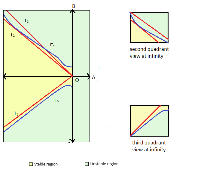
In the second quadrant of the -plane, we observe that the boundary curve has a local minima but no local maxima. As a result, we can find a tangent (in the second quadrant) to , which passes through the origin (denoted as ). After applying the transformations we discussed, the region enclosed by the and the negative -axis will represent the stable region in the -plane. If we consider a line above where and sufficiently small then this line will intersect in two points leading to two critical points and in the SS-region of -plane. As we decrease , the second intersection goes away from the origin and vanishes as we reach (Further details are provided in the subsequent discussion). Thus, the line given by is another boundary in the -plane.
The region bounded by and in the -plane is the SS-region, where we get two critical values and discussed in the previous section. If we decrease further i.e., then the line lies between and the vertical -axis and cuts only at one point. This gives only one critical value of the delay and the region SSR in the -plane.
Also, in the third quadrant, only one branch of the boundary exists. Let us denote by , the tangent line to , passing through the origin. We show that is given by in the following discussion.
So, the region bounded by and negative -axis will be the stable region and the region bounded by and negative -axis will be the
SSR (Single Stable Region) in the -plane after the transformations we discussed (see Figure 6).
4.2 Expressions for
Note that, is tangent to and is tangent to . The line has first intersection with and is tangent to at infinity.
For fixed the equation of tangent to the curve , touching at some point , in parametric form is given by
| (14) |
where .
This tangent line should also pass through the origin, i.e.,
| Eliminating , we get | (15) | ||||
After solving this equation for , we find the slope of tangent line using
| (16) |
Now, by solving (15), we get many values of , but we want the values of v in the intervals and .
-
1.
In (i.e., in the third quadrant), the only permissible value of is for all values of . By putting in (16), we get
Hence, the equation of tangent line is
Using the discussion in this section’s beginning, this tangent becomes in -plane. -
2.
In (i.e., in the second quadrant), we get a bifurcation value such that
- •
-
•
For , which is not constant. Therefore, is also not a constant.
Hence, the equation of tangent line is .The expression for slope is provided in the data set 3.
The bifurcation point can be determined by equating and solving for .
-
3.
Now, is tangent to at its unbounded end.
Note that, becomes unbounded as . Therefore, taking limit in (16), we get Thus, the equation of is given by . will be the corresponding line in the -plane.
-
•
So, and are the same for . Hence, there will be no stability switch for these values of
We present the stability diagrams in -plane in Figure 8, and summarize these results in Theorem 4.1.
Theorem 4.1.
Consider the FDDE
| (17) |
The zero solution of this equation is –
-
1.
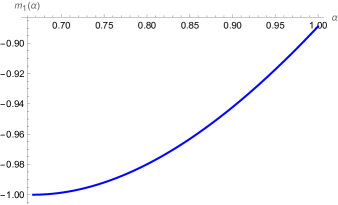
Figure 7: Also, can be approximated as a polynomial of degree 4,i.e.,
-
2.
unstable
-
3.
asymptotically stable for and unstable for , leading to single stable region (SSR), if and , where the critical value is described as below:
If i.e., belongs to the second quadrant then,-
•
If then critical value of delay is given by the intersection of .
-
•
If then we find the point (see data set 1).
– If then will give the critical value of delay.
– If then the critical delay value will be .
If i.e., belongs to the third quadrant, then the critical value will be given by .
The values are given in data set 2. -
•
-
4.
asymptotically stable for , unstable for and again asymptotically stable for , leading to the stability switch (SS), if , and , where is as in case (1) and the constants are mentioned in the data set 2.
5 Illustrative examples
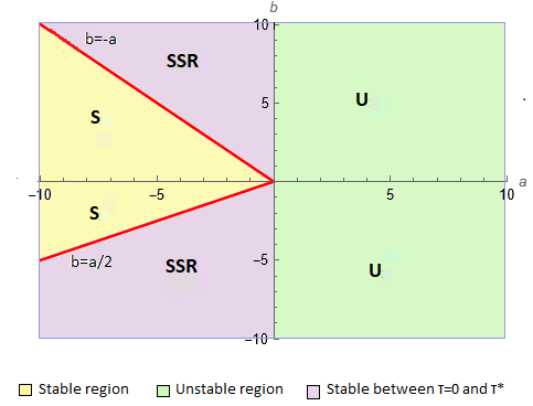
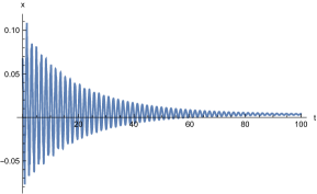
Example 1 Consider the FDDE (5) with . We take different values of and verify the stability regions given in Figure 8(a).
(i)
Consider
Since both . So, region.
Hence, the system is unstable for any .
We sketched an unbounded solution for this case in Figure 9.
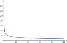
(ii)
Now, consider .
Since SSR.
Furthermore, , thus, based on theorem 4.1, we find the intersection point and get
(see data set 1).
Now,
So, (see data set 2).
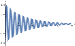
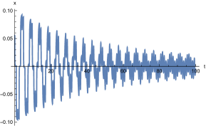
Since , we get the stable solution shown in Figure 10.
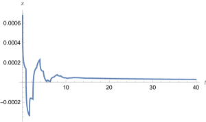
Take the same values of and with .
In this case,
So, (see data set 2).
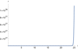
Since , the system is unstable. We get a root with positive real part of the modified characteristic equation (7) supporting this claim.
(iii)
Take .
Since
So,
Hence, we get the stable solution shown in Figure (11).
(iv)
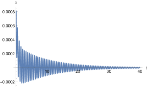
Now, consider and .
Since . So, SSR.
In this case, (see data set 2).
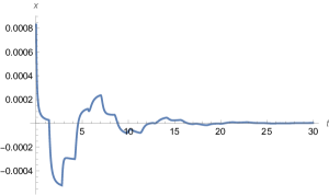
Hence, the system is stable for . We sketched the stable solutions as shown in Figure (12).
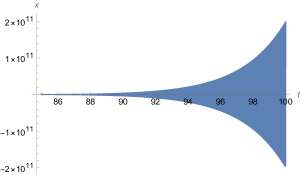
On the other hand, if , then the system is unstable (see Figure 13).
Example 2 Consider the FDDE (5) with . In this case, the stability analysis is provided by Figure 8(b).
(i) If we consider
Then, .
So, region.
Hence, the system is unstable for any . We get an unstable solution shown in Figure 14.
(ii)
Now, take .
Here , so, lies in the SSR region.
Moreover, , so following Theorem 4.1, we determine the intersection point and get (see data set 1).
Now,
So, (see data set 2).
Since , the system will be stable (cf. Figure 15).
Take the same values of and with .
In this case,
So, (see data set 2).
Since , the system is unstable. We get an unstable solution as shown in Figure 16.
(iii)
If we assume .
Here and equation of for is Clearly, the line representing the given value of (a,b) will lie below , i.e., in the stability region.
Hence, the system is stable for any . Stable solutions are sketched in Figure 17.
(iv)
Now, we consider .
Since So,
In this case,
Hence, the system is stable for (cf. Figure 18).
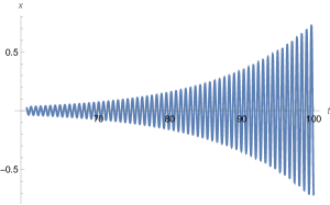
If we consider the same values for and and .
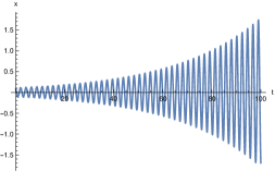
Then, since . The solution trajectory shows unbounded oscillations as shown in Figure 19.
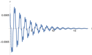
(v)
If we take .
Here , equation of is and equation of is . Hence, the line representing the given value of (a,b) will lie between and i.e., in the region of the stability switch.
So, by putting values of , we will get both the critical values of this region.
and .
So, for , system is stable. Hence, the solution goes to zero as we increase t (see Figure 20).
Now, if i.e , then system will be unstable.
We observed that there is a positive root of the modified characteristic equation (7) validating this assertion.
Also, If we take , then the system is again stable(see Figure 21).
6 Conclusions
We considered the fractional order delay differential equation . We reduced the number of parameters by transforming , . The boundaries of the stable region in the plane are obtained by setting the eigenvalue as a purely imaginary value. This provided stable and unstable regions. Furthermore, we translated these regions to plane. This generated a few more delay-dependent regions, viz. single stable region (SSR), where the system is stable for smaller values of delay and becomes unstable for the larger ones, and stability switch (SS), where we get the intermittent stability behavior as the delay changes. We provided an ample number of examples to support our results. We hope that this work will be an essential step to solve the open problem on the stability analysis of .
Acknowledgment
Pragati Dutta thanks the University of Hyderabad for the non-net fellowship.
References
- [1] Igor Podlubny. Fractional differential equations: an introduction to fractional derivatives, fractional differential equations, to methods of their solution and some of their applications. elsevier, 1998.
- [2] Shantanu Das. Functional fractional calculus, volume 1. Springer, 2011.
- [3] The fundamental solutions for the fractional diffusion-wave equation. Applied Mathematics Letters, 9(6):23–28, 1996.
- [4] A Babakhani and Varsha Daftardar-Gejji. Existence of positive solutions of nonlinear fractional differential equations. Journal of Mathematical Analysis and Applications, 278(2):434–442, 2003.
- [5] Varsha Daftardar-Gejji. Analysis of a system of fractional differential equations. Journal of Mathematical Analysis and Applications, 293(2):511–522, 2004.
- [6] Vangipuram Lakshmikantham and Aghalaya S Vatsala. Basic theory of fractional differential equations. Nonlinear Analysis: Theory, Methods & Applications, 69(8):2677–2682, 2008.
- [7] Bashir Ahmad and Ahmed Alsaedi. Existence and uniqueness of solutions for coupled systems of higher-order nonlinear fractional differential equations. Fixed Point Theory and Applications, 2010:1–17, 2010.
- [8] Yufeng Xu and Zhimin He. Existence and uniqueness results for cauchy problem of variable-order fractional differential equations. Journal of Applied Mathematics and Computing, 43:295–306, 2013.
- [9] YURII Luchko and Rudolf Gorenflo. An operational method for solving fractional differential equations with the caputo derivatives. Acta Math. Vietnam, 24(2):207–233, 1999.
- [10] Sachin Bhalekar and Madhuri Patil. Can we split fractional derivative while analyzing fractional differential equations? Communications in Nonlinear Science and Numerical Simulation, 76:12–24, 2019.
- [11] Changpin Li and Weihua Deng. Remarks on fractional derivatives. Applied mathematics and computation, 187(2):777–784, 2007.
- [12] Kai Diethelm, Neville J Ford, and Alan D Freed. A predictor-corrector approach for the numerical solution of fractional differential equations. Nonlinear Dynamics, 29:3–22, 2002.
- [13] Varsha Daftardar-Gejji, Yogita Sukale, and Sachin Bhalekar. A new predictor–corrector method for fractional differential equations. Applied Mathematics and Computation, 244:158–182, 2014.
- [14] Varsha Daftardar-Gejji and Hossein Jafari. Adomian decomposition: a tool for solving a system of fractional differential equations. Journal of Mathematical Analysis and Applications, 301(2):508–518, 2005.
- [15] S Saha Ray and RK Bera. Analytical solution of the bagley torvik equation by adomian decomposition method. Applied Mathematics and Computation, 168(1):398–410, 2005.
- [16] Varsha Daftardar-Gejji and Hossein Jafari. An iterative method for solving nonlinear functional equations. Journal of mathematical analysis and applications, 316(2):753–763, 2006.
- [17] Ji-Huan He. Homotopy perturbation method: a new nonlinear analytical technique. Applied Mathematics and computation, 135(1):73–79, 2003.
- [18] Denis Matignon. Stability results for fractional differential equations with applications to control processing. In Computational engineering in systems applications, volume 2, pages 963–968. Lille, France, 1996.
- [19] Mohammad Saleh Tavazoei and Mohammad Haeri. Chaotic attractors in incommensurate fractional order systems. Physica D: Nonlinear Phenomena, 237(20):2628–2637, 2008.
- [20] Wajdi M Ahmad and Julien Clinton Sprott. Chaos in fractional-order autonomous nonlinear systems. Chaos, Solitons & Fractals, 16(2):339–351, 2003.
- [21] Chunguang Li and Guanrong Chen. Chaos and hyperchaos in the fractional-order rössler equations. Physica A: Statistical Mechanics and its Applications, 341:55–61, 2004.
- [22] Wei-Ching Chen. Nonlinear dynamics and chaos in a fractional-order financial system. Chaos, Solitons & Fractals, 36(5):1305–1314, 2008.
- [23] Varsha Daftardar-Gejji and Sachin Bhalekar. Chaos in fractional ordered liu system. Computers & mathematics with applications, 59(3):1117–1127, 2010.
- [24] Ivo Petráš and Ivo Petráš. Fractional-order chaotic systems. Fractional-order nonlinear systems: modeling, analysis and simulation, pages 103–184, 2011.
- [25] Eva Kaslik and Seenith Sivasundaram. Nonlinear dynamics and chaos in fractional-order neural networks. Neural networks, 32:245–256, 2012.
- [26] Tianshou Zhou and Changpin Li. Synchronization in fractional-order differential systems. Physica D: Nonlinear Phenomena, 212(1-2):111–125, 2005.
- [27] Weihua Deng. Generalized synchronization in fractional order systems. Physical Review E—Statistical, Nonlinear, and Soft Matter Physics, 75(5):056201, 2007.
- [28] Sachin Bhalekar and Varsha Daftardar-Gejji. Synchronization of different fractional order chaotic systems using active control. Communications in Nonlinear Science and Numerical Simulation, 15(11):3536–3546, 2010.
- [29] Rafael Martínez-Guerra and Claudia Alejandra Pérez-Pinacho. Advances in Synchronization of Coupled Fractional Order Systems: Fundamentals and Methods. Springer, 2018.
- [30] Rudolf Hilfer. Applications of fractional calculus in physics. World scientific, 2000.
- [31] Francesco Mainardi. Fractional calculus and waves in linear viscoelasticity: an introduction to mathematical models. World Scientific, 2022.
- [32] Richard Magin. Fractional calculus in bioengineering, part 1. Critical Reviews™ in Biomedical Engineering, 32(1), 2004.
- [33] Richard L Magin. Fractional calculus models of complex dynamics in biological tissues. Computers & Mathematics with Applications, 59(5):1586–1593, 2010.
- [34] Hal L Smith. An introduction to delay differential equations with applications to the life sciences, volume 57. springer New York, 2011.
- [35] Jack K Hale. Functional differential equations. In Analytic Theory of Differential Equations: The Proceedings of the Conference at Western Michigan University, Kalamazoo, from 30 April to 2 May 1970, pages 9–22. Springer, 2006.
- [36] Muthusamy Lakshmanan and Dharmapuri Vijayan Senthilkumar. Dynamics of nonlinear time-delay systems. Springer Science & Business Media, 2011.
- [37] A Uçar. A prototype model for chaos studies. International journal of engineering science, 40(3):251–258, 2002.
- [38] Michael C Mackey and Leon Glass. Oscillation and chaos in physiological control systems. Science, 197(4300):287–289, 1977.
- [39] Fathalla A Rihan et al. Delay differential equations and applications to biology. Springer, 2021.
- [40] Shigui Ruan. Delay differential equations in single species dynamics. In Delay differential equations and applications, pages 477–517. Springer, 2006.
- [41] Marc R Roussel. The use of delay differential equations in chemical kinetics. The journal of physical chemistry, 100(20):8323–8330, 1996.
- [42] Andrew Keane, Bernd Krauskopf, and Claire M Postlethwaite. Climate models with delay differential equations. Chaos: An Interdisciplinary Journal of Nonlinear Science, 27(11), 2017.
- [43] Rebecca V Culshaw and Shigui Ruan. A delay-differential equation model of hiv infection of cd4+ t-cells. Mathematical biosciences, 165(1):27–39, 2000.
- [44] Sachin Bhalekar. Stability and bifurcation analysis of a generalized scalar delay differential equation. Chaos: An Interdisciplinary Journal of Nonlinear Science, 26(8), 2016.
- [45] Sachin B Bhalekar. Stability analysis of a class of fractional delay differential equations. Pramana, 81(2):215–224, 2013.
- [46] Sachin Bhalekar and Deepa Gupta. Stability and bifurcation analysis of a fractional order delay differential equation involving cubic nonlinearity. Chaos, Solitons & Fractals, 162:112483, 2022.
- [47] Sachin Bhalekar and Deepa Gupta. Can a fractional order delay differential equation be chaotic whose integer-order counterpart is stable? In 2023 International Conference on Fractional Differentiation and Its Applications (ICFDA), pages 1–6. IEEE, 2023.
- [48] Sachin Bhalekar and Deepa Gupta. Stability and bifurcation analysis of two-term fractional differential equation with delay. arXiv preprint arXiv:2404.01824, 2024.
- [49] Deepa Gupta and Sachin Bhalekar. Fractional order sunflower equation: Stability, bifurcation and chaos. arXiv preprint arXiv:2404.17321, 2024.
- [50] SACHIN Bhalekar and VARSHA Daftardar-Gejji. A predictor-corrector scheme for solving nonlinear delay differential equations of fractional order. J. Fract. Calc. Appl, 1(5):1–9, 2011.
- [51] Varsha Daftardar-Gejji, Yogita Sukale, and Sachin Bhalekar. Solving fractional delay differential equations: a new approach. Fractional Calculus and Applied Analysis, 18:400–418, 2015.
- [52] Sachin Bhalekar and Varsha Daftardar-Gejji. Fractional ordered liu system with time-delay. Communications in Nonlinear Science and Numerical Simulation, 15(8):2178–2191, 2010.
- [53] Sachin Bhalekar. Dynamical analysis of fractional order uçar prototype delayed system. Signal, Image and Video Processing, 6:513–519, 2012.
- [54] Liguo Yuan, Qigui Yang, and Caibin Zeng. Chaos detection and parameter identification in fractional-order chaotic systems with delay. Nonlinear Dynamics, 73:439–448, 2013.
- [55] Zhen Wang, Xia Huang, and Guodong Shi. Analysis of nonlinear dynamics and chaos in a fractional order financial system with time delay. Computers & Mathematics with Applications, 62(3):1531–1539, 2011.
- [56] Sachin Bhalekar, Varsha Daftardar-Gejji, Dumitru Baleanu, and Richard Magin. Fractional bloch equation with delay. Computers & Mathematics with Applications, 61(5):1355–1365, 2011.
- [57] Anne Beuter, Jacques Bélair, Christiane Labrie, and Jacques Bélair. Feedback and delays in neurological diseases: A modeling study using gynamical systems. Bulletin of mathematical biology, 55:525–541, 1993.
- [58] Anne Beuter, David Larocque, and Leon Glass. Complex oscillations in a human motor system. Journal of motor behavior, 21(3):277–289, 1989.
- [59] Monika Joanna Piotrowska. Hopf bifurcation in a solid avascular tumour growth model with two discrete delays. Mathematical and Computer Modelling, 47(5-6):597–603, 2008.
- [60] Jacques Bélair, Michael C Mackey, and Joseph M Mahaffy. Age-structured and two-delay models for erythropoiesis. Mathematical biosciences, 128(1-2):317–346, 1995.
- [61] RD Braddock and P Van den Driessche. On a two lag differential delay equation. The ANZIAM Journal, 24(3):292–317, 1983.
- [62] JACK K Hale and WZ Huang. Global geometry of the stable regions for two delay differential equations. Journal of Mathematical analysis and applications, 178(2):344–362, 1993.
- [63] Joseph M Mahaffy, Kathryn M Joiner, and Paul J Zak. A geometric analysis of stability regions for a linear differential equation with two delays. International Journal of Bifurcation and Chaos, 5(03):779–796, 1995.
- [64] Xiangao Li, Shigui Ruan, and Junjie Wei. Stability and bifurcation in delay–differential equations with two delays. Journal of Mathematical Analysis and Applications, 236(2):254–280, 1999.
- [65] Roger D Nussbaum. Differential-delay equations with two time lags, volume 205. American Mathematical Soc., 1978.
- [66] Sachin Bhalekar. Analysing the stability of a delay differential equation involving two delays. Pramana, 93:1–7, 2019.
- [67] Stefan G Samko. Fractional integrals and derivatives. Theory and applications, 1993.
- [68] Weihua Deng, Changpin Li, and Jinhu Lü. Stability analysis of linear fractional differential system with multiple time delays. Nonlinear Dynamics, 48:409–416, 2007.