Reinforcement Leaning for Infinite-Dimensional Systems

Abstract

Interest in reinforcement learning (RL) for massive-scale systems consisting of large populations of intelligent agents interacting with heterogeneous environments has witnessed a significant surge in recent years across diverse scientific domains. However, due to the large-scale nature of the system, the majority of state-of-the-art RL techniques either encounter high computational cost or exhibit compromised performance. To mitigate these challenges, we propose a novel RL architecture along with the derivation of effective algorithms to learn optimal policies for any arbitrarily large system of agents. Specifically, we model such a system as a parameterized control system defined on an infinite-dimensional function space. We then develop a moment kernel transform to map the parameterized system and the value function of an RL problem into a reproducing kernel Hilbert space. This transformation subsequently generates a finite-dimensional moment representation for this RL problem. Leveraging this representation, we develop a hierarchical algorithm for learning optimal policies for the infinite-dimensional parameterized system. We further enhance efficiency of the algorithm by exploiting early stopping at each hierarchy, by which we show the fast convergence property of the algorithm through constructing a convergent spectral sequence. The performance and efficiency of the proposed algorithm are validated using practical examples.

Keywords: Reinforcement learning, parameterized systems, moment kernelization, spectral sequence convergence, control theory

1 Introduction

Reinforcement learning (RL), a prominent machine learning paradigm, has gained recognition as a powerful tool for intelligent agents to learn optimal policies. These policies guide the agents’ decision-making processes toward achieving desired goals by maximizing the expected cumulative rewards. RL exhibits a wide range of applications across various domains, encompassing robotics, game-playing, recommendation systems, autonomous vehicles, and control systems. In this decade, learning optimal policies to manipulate the behavior of large-scale systems of intelligent agents interacting with different environments has attracted increasing attention and is gradually becoming a recurrent research theme in RL society. Existing and potential applications of “large-scale RL” include targeted coordination of robot swarms for motion planning in robotics (Becker and Bretl, 2012; Shahrokhi et al., 2018), desynchronization of neuronal ensembles with abnormal oscillatory activity for the treatment of movement disorders, e.g., Parkinson’s disease, epilepsy, and essential tremor, in neuroscience and brain medicine (Marks, 2005; Wilson, 2005; Shoeb, 2009; Zlotnik and Li, 2012; Li et al., 2013; Vu et al., 2024), and robust excitation of nuclear spin samples for nuclear magnetic resonance (NMR) spectroscopy and magnetic resonance imaging (MRI) in quantum science (Glaser et al., 1998; Li et al., 2011; Dong et al., 2008; Chen et al., 2014).

The fundamental challenge to these RL tasks unarguably lies in the massive scale of these agent systems as well as the dynamic environments where the agents take actions. For example, a neuronal ensemble in the human brain may comprise up to $\sim 10^{11}$ neuron cells (Herculano-Houzel, 2012; Ching and Ritt, 2013) and a spin sample in an NMR experiment typically consists of $\sim 10^{23}$ nuclear spins (Li, 2006; Cavanagh et al., 2010; Li, 2011). Although, mathematically speaking, these systems are composed of finitely many agents, it is more appropriate to treat them as infinite agent populations. This is because their massive scale disables the possibility to specifically identifying and making decisions for each individual agent in these populations. These restrictions particularly imply that such policy learning tasks exceed the capability of classical multi-agent RL methods, which are concerned with learning joint policies providing each agent with a customized action based on the states of all the other agents (Littman, 1994; Foerster et al., 2016; Gupta et al., 2017; Zhang et al., 2021b; Albrecht et al., 2024). Consequently, all the agents in such a population are forced to take the same action so that it is necessary to learn and implement policies at the population level. In addition, natural models describing the dynamic behavior of these intelligent agents typically take the form of continuous-time deterministic control systems. Learning optimal policies for this category of systems also lies outside the scope of most state-of-the-art and benchmark RL algorithms, notably Trust Region Policy Optimization (TRPO) and Proximal Policy Optimization (PPO) (Schulman et al., 2017, 2015), based on Markov decision processes, which are discrete-time stochastic control processes. This in turn stresses the urgent demand for a more inclusive RL framework that accommodates policy learning tasks for infinite agent populations in the continuous-time and deterministic setting.

Our contributions.

This work is devoted to developing a novel RL architecture that enables the derivation of effective algorithms to learn optimal policies for population systems consisting of infinitely many intelligent agents interacting with heterogeneous dynamic environments. We formulate such an agent system as a parameterized control system, in which each individual system indexed by a specific parameter value represents the environment of an agent in the population. We then evolve this parameterized system on an infinite-dimensional function space and carry out a functional setting for RL of this infinite-dimensional dynamical system. The primary tool that we develop to tackle this RL problem is the moment kernel transform. Specifically, it maps the parameterized system and its value function to a control system and a value function defined on a reproducing kernel Hilbert space (RKHS) consisting of moment sequences, yielding a kernel parameterization of the RL problem. In particular, the kernelization of the parameterized system in terms of moment sequences directly enables the finite-dimensional truncation approximation of the moment kernelized system. As a result, optimal policy learning for the infinite-dimensional parameterized system can be facilitated by RL of the finite-dimensional truncated moment kernelized system. Based on this, we develop a hierarchical policy learning algorithm for the parameterized system, in which each hierarchy consists of an RL problem for a finite-dimensional truncated moment kernelized system. We further provide the convergence guarantee of the algorithm in the sense that the policies learned from a sequence of truncated moment kernelized systems with increasing truncation orders converge to the optimal policy of the parameterized system. To enhance the computational efficiency of the proposed algorithm, we also explore early stopping criteria for the finite-dimensional RL problem in each hierarchy and then prove the convergence of the hierarchical algorithm with early-stopped hierarchies in terms of spectral sequences. The performance and efficiency of the proposed hierarchical policy learning algorithm are demonstrated by using examples arising from practical applications. The contributions of our work are summarized as follows.

• Formulation of infinite intelligent agent populations as parameterized systems defined on infinite-dimensional function spaces.

• Development of the moment kernel transform that gives rise to a kernel parameterization of RL problems for parameterized systems in terms of moment sequences in an RKHS.

• Design of a hierarchical policy learning algorithm for RL of parameterized systems with convergence guarantees.

• Exploration of early stopping criteria for each hierarchy in the proposed hierarchical algorithm and proof of the spectral sequence convergence of the hierarchical algorithm with early-stopped hierarchies.

Related works.

Learning control policies to coordinate large intelligent agent populations by using RL approaches has been witnessed to attract increasing attention in recent years. Such large-scale and high-dimensional RL problems arise from numerous emerging applications, including game playing (Silver et al., 2017, 2018; Vinyals et al., 2019; OpenAI et al., 2019; Schrittwieser et al., 2020; Kaiser et al., 2020), human-level decision making (Mnih et al., 2015; Liu et al., 2022; Baker et al., 2020), and control of multi-agent systems (Buşoniu et al., 2010; Heredia and Mou, 2019; Jiang et al., 2021; Zhang et al., 2021b; Albrecht et al., 2024), particularly, many-body quantum systems (Dong et al., 2008; Lamata, 2017; Bukov et al., 2018; Haug et al., 2021) and multi-robot systems (Matarić, 1997; Long et al., 2018; Yang et al., 2020; Yang and Gu, 2004; Lu et al., 2024).

One of the most active research focuses regarding large-scale and high-dimensional policy learning problems is placed on deep RL, which incorporates deep learning techniques, particularly the use of deep neural networks, into RL algorithms (Bertsekas and Tsitsiklis, 1996; François-Lavet et al., 2018; Bellemare et al., 2020; Nakamura-Zimmerer et al., 2021; Le et al., 2022; Sarang and Poullis, 2023). However, it is common knowledge that training deep neural networks to tackle high-dimensional learning problems can be computationally expensive. Effective approaches to address this issue include developing distributed RL algorithms (Heredia and Mou, 2019; Heredia et al., 2020; Yazdanbakhsh et al., 2020; Heredia et al., 2022; Xie et al., 2024) and learning compact representations of high-dimensional measurement data (Momennejad et al., 2017; Gelada et al., 2019; Laskin et al., 2020; Zhang et al., 2021a).

In these existing works, the scale of the intelligent agent populations varies from tens to thousands. However, allowing the number of agents in a population to be arbitrarily large, in the limit to approach infinity, as considered in this work remains under-explored with sparse literature in the RL society. Moreover, the formulation of RL problems over infinite-dimensional spaces has only been proposed in the stochastic setting, to learn feedback control policies for stochastic partial differential equation systems by using variational optimization methods (Evans et al., 2020).

The major technical tool developed in the work to address the curse of dimensionality is the moment kernel transform, which is inspired by the method of moments. This method was developed by the Russian mathematician P. L. Chebyshev in 1887 to prove the law of large numbers and central limit theorem (Mackey, 1980). Since then, the method has been extensively studied under different settings, notably, the Hausdorff, Hausdorff, and Stieltjes moment problems (Hamburger, 1920, 1921a, 1921b; Hausdorff, 1923; Stieltjes, 1993). The most general formulation in modern terminologies was proposed by the Japanese mathematician Kōsaku Yosida (Yosida, 1980). Recently, the method of moments was introduced to control theory for establishing dual representations of ensemble systems (Narayanan et al., 2024) and machine learning-aided medical decision making as a feature engineering technique (Yu et al., 2023). These two works, together with Yosida’s formulation of the moment problem, lay the foundation for the development of the moment kernel transform.

2 Policy Learning for Massive-Scale Dynamic Populations

This section mainly devotes to establishing a general formulation for RL of infinite populations of intelligent agents interacting with heterogeneous environments described by continuous-time control systems. Specifically, we start with demonstrating the challenges to such RL tasks, which in turn motivates the modeling of these populations as parameterized control systems defined on infinite-dimensional function spaces. Then, we carry out a functional setting for RL of parameterized systems and delve into establishing the theoretical foundations, particularly, conditions guaranteeing the existence of optimal policies for such infinite-dimensional systems.

2.1 Challenges to reinforcement learning of large-scale dynamic populations

Learning control policies for a large-scale population of, in the limit a continuum of, intelligent agents, described by continuous-time deterministic dynamical systems, presents significant challenges to reinforcement learning (RL). Primarily, the massive population size makes RL algorithms implement on high-dimensional spaces so that the notorious curse of dimensionality arises, leading to high computational costs and low learning accuracy (Bellman et al., 1957; Bellman, 1961; Sutton and Barto, 2018). Moreover, the continuous-time deterministic system formulation is not consistent with the setting of most state-of-the-arts RL algorithms, which are typically based on Markov decision processes, those are, discrete-time stochastic control processes.

To further demonstrate these challenges by using an illustrative example, we consider a population consisting of $n$ time-invariant scalar linear systems controlled by a common policy, give by, $\frac{d}{dt}x_{i}(t)=a_{i}x(t)+u(t)$, where $x_{i}(t)\in\mathbb{R}$ is the state of the $i^{\rm th}$ system, $u(t)\in\mathbb{R}$ is the control policy, and $a_{i}\in\mathbb{R}$ and $i=1,\dots,n$. Equivalently, the entire population can be represented as an $n$-dimensional linear system $\frac{d}{dt}x(t)=Ax(t)+Bu(t)$, where $x(t)=[\,x_{1}(t),\dots,x_{n}(t)\,]^{\prime}\in\mathbb{R}^{n}$ is the state with ’$\prime$’ denoting the transpose of vectors (and matrices), $A\in\mathbb{R}^{n\times n}$ is the diagonal matrix with the $(i,i)$-entry given by $a_{i}$ for all $i=1,\dots,n$, and $B\in\mathbb{R}^{n}$ is vector of ones. In particular, $a_{1}$, $\dots$, $a_{n}$ are uniformly sampled from $[-1,1]$, i.e., $a_{i}=-1+2(i-1)/(n-1)$ for each $i=1,\dots,n$, and the RL task is to learn the infinite-time horizon linear quadratic regulator (LQR) with the cumulative reward $V(x(t))=\int_{t}^{\infty}e^{-2.5t}[x^{\prime}(t)x(t)/n+u^{2}(t)]dt$. It is well-known that the value function $V^{*}(x(t))=\inf_{u}V(x(t))$ is in the quadratic form $V^{*}(x(t))=x^{\prime}(t)Qx(t)$ parameterized by a positive definite matrix $Q\in\mathbb{R}^{n\times n}$ (Brockett, 2015). Therefore, the value iteration stands out as the prime RL algorithm to tune the $n(n+1)/2$ training parameters in $Q$ to learn the LQR policy and value function (Sutton and Barto, 2018; Bertsekas, 2019).

Curse of dimensionality.

In the simulation, we vary the dimension $n$ of the system from 2 to 20. Figure 1(a) shows the number of training parameters (the top panel) and computational time (the bottom panel) with respect to $n$, both of which grow dramatically when $n$ increases. In addition to these common consequences of the curse of dimensionality, we also observe a convergence issue of RL when the dimension $n$ becomes high.

Convergence issue.

Note that by the definition of Riemann integrals (Rudin, 1976), the cumulative reward satisfies the convergence property

$$V(x(t))=\int_{t}^{\infty}e^{-2.5t}\Big{[}\sum_{i=1}^{n}x_{i}^{2}(t)/n+u^{2}(t)\Big{]}dt\rightarrow\int_{t}^{\infty}e^{-2.5t}\Big{[}\int_{-1}^{1}x^{2}(t,\beta)d\beta+u^{2}(t)\Big{]}dt$$ (1)

as $n\rightarrow\infty$, where $x(t,\beta)$ satisfies the linear system

$$\frac{d}{dt}x(t,\beta)=\beta x(t,\beta)+u(t)$$ (2)

on $\mathbb{R}$ for all $\beta\in[-1,1]$. Therefore, the value function necessarily inherits the convergence property as $n\rightarrow\infty$ due to the fact that taking infimum preserves lower semicontinuity of functions (Folland, 2013). Let $V_{n}^{*}$ and $u_{n}^{*}$ denote the value function and LQR policy learned from the $n$-dimensional system, then as shown in Figure 1(b), neither $\|V_{n}^{*}-V_{n-1}^{*}\|=\sup_{t\geq 0}|V_{n}^{*}(x^{*}(t))-V_{n-1}(x^{*}(t))|$ nor $\|u_{n}^{*}-u_{n-1}^{*}\|=\sup_{t\geq 0}|u_{n}^{*}(t)-u_{n-1}^{*}(t)|$ converges to 0, where $x^{*}(t)$ denotes the optimal trajectory. This particularly fails to verify the convergence of the value function, which further raises the convergence issue of standard RL algorithms when applied to high-dimensional systems.

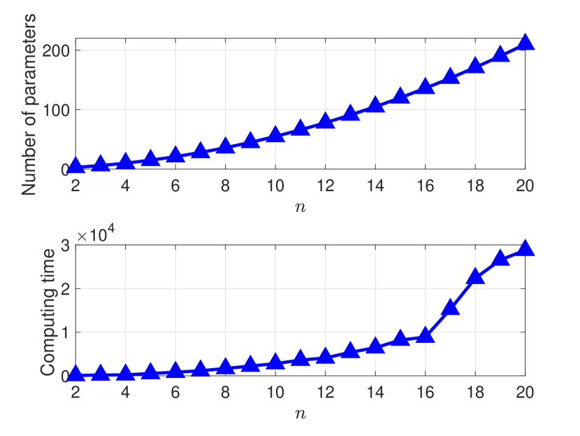
(a)

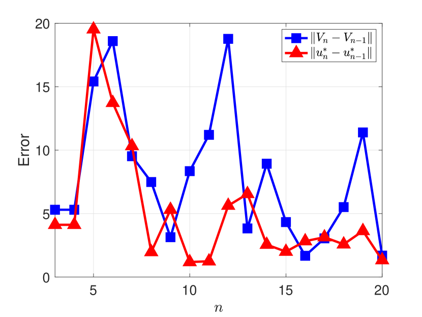
(b)

Figure 1: Illustration of the challenges to RL for high-dimensional systems. The standard value iteration is applied to learn the LQR policy and value function for an $n$-dimensional time-invariant deterministic linear system, with $n$ ranging from 2 to 20. In particular, (a) shows the number of training parameters (top) and computing time (bottom) with respect to the system dimension $n$, and (b) plots the distance between successive terms in the sequences of the learned value functions (blue) and LQR policies (red) with respect to $n$.

The purpose of this work is to develop a new RL structure to address these challenges. To pave the way for this, we will first introduce a principled RL formulation for large-scale population systems, regardless of the population size.

2.2 Reinforcement learning for parameterized systems on function spaces

The convergence argument carried out in (2) inspires the modeling of a population of intelligent agents in terms of a parameterized differential equation system, given by

$$\frac{d}{dt}x(t,\beta)=F(t,\beta,x(t,\beta),u(t)),$$ (3)

where $\beta$ is the system parameter taking values on $\Omega\subseteq\mathbb{R}^{d}$, $x(t,\beta)\in M$ is the state of the “$\beta$-th” system (the environment of the “$\beta$-th” agent) in the population with $M\subseteq\mathbb{R}^{n}$ a differentiable manifold, $u(t)\in\mathbb{R}^{r}$ is the common control policy, and $F(t,\beta,\cdot,u(t))$ is a (time-varying) vector field on $M$ for each $\beta\in\Omega$ and $u(t)\in\mathbb{R}^{r}$. One of the major advantages of the parameterized system formulation is the ability to model population systems of any size, in the limit a continuum of systems when the parameter space $\Omega$ has an uncountable cardinality. Indeed, the state of the parameterized system in (3) gives rise to a function $x(t,\cdot):\Omega\rightarrow M$ so that the system is evolving on $\mathcal{F}(\Omega,M)$, a space of $M$-valued functions defined on $\Omega$.

Similarly, as motivated in (1), it is appropriate to associate the parameterized system in (3) with a cumulative reward in the integral form as

$$V(t,x_{t})=\int_{\Omega}\Big{[}\int_{t}^{T}r(s,x(s,\beta),u(s))ds+K(T,x(T,\beta))\Big{]}d\beta,$$ (4)

with $x_{t}(\cdot)=x(t,\cdot)$. This integral reward is essentially the “average” of the cumulative rewards of all the individual systems in the population and hence connotes a manifestation of the collective behavior of the entire population. Note that for each $t$, the cumulative reward is essentially a functional on $\mathcal{F}(\Omega,M)$, and hence RL problems for the parameterized system in (1) are policy learning tasks over the function space $\mathcal{F}(\Omega,M)$. However, $\mathcal{F}(\Omega,M)$ is generally an infinite-dimensional manifold, and this poses significant challenges to such learning problems, which are also beyond the scope of many existing RL algorithms. To guarantee solvability of such demanding leaning tasks, some regularity conditions on the system dynamics $F$, immediate reward $r$, and terminal cost $K$ are expected.

Assumption S1.

(Boundedness of control policies) The ensmeble control policy $u:[0,T]\rightarrow\mathbb{R}^{m}$ is a measurable function and takes values on a compact subset $U$ of $\mathbb{R}^{m}$.

Assumption S2.

(Lipschitz continuity of system dynamics) The vector field $F:\mathbb{R}\times\Omega\times M\times U\rightarrow TM$ is continuous in all of the variables and Lipschitz continuous in $z\in M$ uniformly for $(t,\beta,a)\in[0,T]\times\Omega\times U$, that is, there exists a constant $C$ (independent of $t\in[0,T]$, $\beta\in\Omega$, and $a\in U$) such that $|(\varphi_{*}F|_{V})(t,\beta,\varphi(p),a)-(\varphi_{*}F|_{V})(t,\beta,\varphi(q),a)|\leq C|\varphi(p)-\varphi(q)|$ for any $p,q\in V$ and coordinate chart $(V,\varphi)$ on $M$, where $TM$ denotes the tangent bundle of $M$, $\varphi_{*}F|_{V}$ denotes the pushforword of $F|_{V}$, the restriction of the vector field $F$ on $V\subseteq M$, and $|\cdot|$ denotes a norm on $\mathbb{R}^{n}$.

According to the theory of ordinary differential equations, this assumption guarantees that, driven by any admissible control policies, each individual system in the ensemble in (3) has a unique and Lipschitz continuous solution (Arnold, 1978; Lang, 1999). Correspondingly, from the functional perspective, as $\beta$ varies on $\Omega$, the ensemble system has a unique solution on $\mathcal{F}(\Omega,M)$.

Assumption C1.

(Integrability of cumulative rewards) There exists an ensemble control policy $u\in\mathcal{U}$ such that $\int_{\Omega}\int_{0}^{T}|r(t,x(t,\beta),u(t))|dtd\beta+\int_{\Omega}|K(T,x(T,\beta))|d\beta<\infty$, where $x(t,\cdot)\in\mathcal{F}(\Omega,M)$ is the solution of the ensemble system in (3) driven by $u$.

Assumption C2.

(Lipschitz continuity of cumulative rewards) Both the running cost $r:\mathbb{R}\times M\times U\rightarrow\mathbb{R}$ and terminal cost $K:\mathbb{R}\times M\rightarrow\mathbb{R}$ are continuous functions in all the variables and Lipschitz continuous in $z\in M$ for any $(t,a)\in[0,T]\times U$.

This regularity assumptions then guarantees the existence of the solution to the infinite-dimensional RL problem for the parameterized system in (3) with cumulative rewards given by (4), equivalently, the value function $V^{*}(t,x_{t})=\inf_{u}V(t,x_{t})$ is well-defined. To emphasize the dependence of the cumulative reward $V$ on the policy $u$, we write $V(0,x_{0})=J(u)$, which gives real-valued function $J$, also refered to as the cost functional, defined on the space of admissible policies $\mathcal{U}=\{u:[0,T]\rightarrow\mathbb{R}^{r}\mid u(t)\in U\}$. The solvability of the RL problem is then based on compactness of $\mathcal{U}$ and continuity of $J$.

Lemma 1

The space of admissible policies $\mathcal{U}$ is compact.

Proof  Topologically, $\mathcal{U}$, equipped with the topology of pointwise convergence, is essentially the product space $\prod_{t\in[0,T]}U$ under the product topology. Because $U\subset\mathbb{R}^{m}$ is a compact by Assumption 1, the compactness of $\mathcal{U}$ directly follows from Tychonoff’s theorem (Munkres, 2000).  

Lemma 2

The cost functional $J:\mathcal{U}\rightarrow\mathbb{R}$ is sequentially continuous, that is, $J(u_{k})\rightarrow J(u)$ for any sequence $(u_{k})_{k\in\mathbb{N}}$ in $\mathcal{U}$ such that $u_{k}\rightarrow u$.

Proof  See Appendix A.  

Theorem 3 (Existence of optimal policies)

Given a parameterized system defined on the function space $\mathcal{F}(\Omega,M)$ as in (3) satisfying Assumptions S1 and S2 and the cumulative reward as in (4), in which the immediate reward $r:\mathbb{R}\times M\times U\rightarrow\mathbb{R}$ and terminal cost $K:\mathbb{R}\times M\rightarrow\mathbb{R}$ satisfying Assumptions C1 and C2. Then, the value function $V^{*}:[0,T]\times\mathcal{F}(\Omega,M)\rightarrow\mathbb{R}$, given by $V^{*}(t,x_{t})=\inf_{u}V(t,x_{t})$, is well-defined, equivalently, the optimal policy exists.

Proof  By the uniqueness of the solution to the parameterized differential equation guaranteed by Assumptions S1 and S2, the policy minimizing $J$ also minimizes $V(t,x_{t})$ for all $t\in[0,T]$. Therefore, it suffices to show the existence of the minimizer of $J$.

Without loss of generality, we assume that the integrability condition in Assumption C1 is satisfied for all $u\in\mathcal{U}$, then it suffices to show that the range $J(\mathcal{U})$ of the cost functional $J$ is a compact space of $\mathbb{R}$, which is equivalent to the sequential compactness, that is, any sequence in $J(\mathcal{U})$ has a convergent subsequence, because of $J(\mathcal{U})\subseteq\mathbb{R}$ (Munkres, 2000).

Pick an arbitrary sequence $(J_{k})_{k\in\mathbb{N}}$ in $J(\mathcal{U})$, which also gives a sequence $(u_{k})_{k\in\mathbb{N}}$ in $\mathcal{U}$ such that $J(u_{k})=J_{k}$. Then, the sequence $(u_{k})_{k\in\mathbb{N}}$ has an accumulation point at some $u\in\mathcal{U}$. To see this, we define $T_{k}=\{x_{n}:n\geq k\}$, then $\bigcap_{k\in\mathbb{N}}\overline{T}_{k}\neq\varnothing$ holds, where $\overline{T}_{n}$ denotes the closure of $T_{n}$. Otherwise, $\{\mathcal{U}\backslash\overline{T}_{k}\}_{k\in\mathbb{N}}$ forms an open cover of $\mathcal{U}$, which then has a finite subcover, say $\mathcal{U}=\bigcap_{k=1}^{N}(\mathcal{U}\backslash\overline{T}_{k})$ due to the compactness of $\mathcal{U}$ as shown in Lemma 1, leading to the contradiction $\varnothing=\mathcal{U}\backslash\big{(}\bigcap_{k=1}^{N}(\mathcal{U}\backslash\overline{T}_{k})\big{)}=\bigcap_{k=1}^{N}\overline{T}_{k}=\overline{T}_{N}$. Now, let $u\in\bigcap_{k\in\mathbb{N}}\overline{T}_{k}$ and $W$ be a neighborhood of $u$, then $W\cap T_{k}\neq\varnothing$ for every $k$, i.e., $W$ contains some $u_{k}$ for any arbitrarily large $k$, and hence $u$ is necessarily an accumulation point of the sequence $(u_{k})_{k\in\mathbb{N}}$.

Be Lemma 2, because $J$ is sequentially continuous, i.e., mapping convergent sequences in $\mathcal{U}$ to convergent sequences in $\mathbb{R}$, it must map the accumulation point $u$ to an accumulation point $J(u)$ of the sequence $(J_{k})_{k\in\mathbb{N}}$. As a result, there is a subsequence of $(J_{k})_{k\in\mathbb{N}}$ converges to $J(u)$, showing the sequential compactness, and hence also compactness, of $J(\mathcal{U})$.  

Although Theorem 3 is to theoretically verify the solvability of the RL problem over the infinite-dimensional function space, the main idea of the employed topological argument exactly coincides with the actor-critic algorithm. Specifically, the “critic” $J$ keeps evaluating the “actor” $u$ for iteratively improving its performance, which generates a policy sequence $u_{k}$ so that $J_{k}=J(u_{k})$ converges to the minimum cost, yielding the optimal policy as well. This actor-critic type procedure also avoids a technical issue to the search of the optimal policy: even though $\mathcal{U}$ is compact, the policy sequence $u_{k}$ may not contain any convergent subsequence since $\mathcal{U}$ is not a first-countable space (Munkres, 2000).

3 Reinforcement Learning of Parameterized Systems in the Moment Kernel Parameterization

Starting from this section, we will focus on the development of an RL framework for learning optimal policies of parameterized ensemble systems defined on infinite-dimensional function spaces. The initial step, as well as an essential step to most learning problems, is to explore an appropriate parameterization for the learning targets. In our case, we will introduce a moment kernel transform, which maps paramterized systems and their cumulative rewards to control systems and functions, respectively, defined on a reproducing kernel Hilbert space (RKHS), giving rise to a kernel parameterization of the RL problems.

3.1 Moment kernelization of parameterized systems and value functions on function spaces

Moment kernelization of parameterized systems.

To motivate the idea and to be consistent with the general formulation of the moment problem proposed by Yosida (Yosida, 1980), we consider the case that the function state-space $\mathcal{F}(\Omega,M)$ of the parameterized system in (3), that is,

$$\frac{d}{dt}x(t,\beta)=F(t,\beta,x(t,\beta),u(t)),\quad\beta\in\Omega,$$

is a Hilbert space $\mathcal{H}$ consisting of real-valued functions defined on $\Omega\subseteq\mathbb{R}^{d}$. We further assume that $\mathcal{H}$ is separable, as a result of which $\mathcal{H}$ has a countable orthonormal basis $\{\Phi_{k}\}_{k\in\mathbb{N}}$ (Yosida, 1980). Then, we define the $k^{\rm th}$ moment associated with the parameterized system in (3) by

$$m_{k}(t)=\langle\Phi_{k},x_{t}\rangle,$$ (5)

where $\langle\cdot,\cdot\rangle:\mathcal{H}\times\mathcal{H}\rightarrow\mathbb{R}$ denotes the inner product on $\mathcal{H}$. Notationally, we use $m(t)$ to denote the moment sequence $(m_{k}(t))_{k\in\mathbb{N}}$ associated with the state $x_{t}\in\mathcal{H}$ and $\mathcal{M}$ to denote the space of all moment sequences, also referred to as the moment space. Specifically, owing to the integrability assumption in Assumption C1, we are particularly interested in the case that $\mathcal{H}$ is a subspace of $L^{2}(\Omega)$, the space of square integrable functions defined on $\Omega$ with respect to the Lebesgue measure, with the inner product given by $m_{k}(t)=\langle\Phi_{k},x_{t}\rangle=\int_{\Omega}\Phi_{k}(\beta)x_{t}(\beta)d\beta$.

Due to orthogonality of the basis $\{\Phi_{k}\}_{k\in\mathbb{N}}$, Parseval’s identity implies $\sum_{k\in\mathbb{N}}|m_{k}(t)|^{2}=\|m(t)\|=\|x_{t}\|=\int_{\Omega}|x_{t}(\beta)|^{2}d\beta<\infty$ so that $\mathcal{M}$ is Hilbert subspace of $\ell^{2}$, the space of square-summable sequences, and the moment transform is an isometric isomorphism between $\mathcal{H}$ and $\mathcal{M}$ (Folland, 2013). It is well-known that $\ell^{2}$ is an RKHS, and hence as a subspace of $\ell^{2}$, $\mathcal{M}$ also inherits the RKHS structure (Paulsen and Raghupathi, 2016). Therefore, moment sequences in $\mathcal{M}$ give rise to a kernel parameterization of functions in $\mathcal{H}$ where the parameterized system evolves on.

To further kernelize the parameterized system, we derive the differential equation governing the time-evolution of the moment sequence as

$$\frac{d}{dt}m_{k}(t)=\frac{d}{dt}\langle\Phi_{k},x_{t}\rangle=\Big{\langle}\Phi_{k},\frac{d}{dt}x_{t}\Big{\rangle}=\langle\Phi_{k},F(t,\cdot,x_{t},u(t))\rangle,$$ (6)

where the change of the order of the time-derivative and inner product operation follows from the dominant convergence theorem (Folland, 2013). Note that because the state-space $\mathcal{H}$ of the parameterized system is a vector space, the vector field $F(t,\beta,x_{t}(\beta),u(t))$ governing the system dynamics, considered as a function in $\beta$, is necessarily an element of $\mathcal{H}$ as well. Comparing the term $\langle\Phi_{k},F(t,\cdot,x_{t},u(t))\rangle$ in (6) with the definition of the $k^{\rm th}$-moment in (5), we observe that this term is essentially the $k^{\rm th}$ moment of $F(t,\cdot,x_{t},u(t))$ as a function on $\mathcal{H}$. Let $\bar{F}(t,m(t),u(t))$ denote the moment sequence of $F(\beta,x(t,\beta),u(t))$, we obtain a concrete representation of the moment system defined on $\mathcal{M}$ as

$$\frac{d}{dt}m(t)=\bar{F}(t,m(t),u(t)).$$ (7)

Remark 4

Note that the moment kernelized system in (7) always consists of countably many components, even though the parameterized system in (3) may represent a continuum of (uncountably many) intelligent agents. This implies that the moment kernelization not only defines a kernel parameterization but also a model reduction for parameterized systems. This feature of the moment kernelization will be fully exploited in the development of the RL framework for learning optimal policies of parameterized systems.

Moment kernelization of value functions.

To establish an RL environment in the moment domain, it remains to kernelize the cumulative reward $V:[0,T]\times\mathcal{H}\rightarrow\mathbb{R}$. To this end, we notice that the integrability condition in Assumption C1 implies the applicability of Fubini’s theorem to change the order of the two integrals in the first summand of $V$ (Folland, 2013), resulting in $V(t,x_{t})=\int_{t}^{T}\int_{\Omega}r(s,x(s,\beta),u(s))d\beta ds+\int_{\Omega}K(T,x(T,\beta))d\beta$. Observe that, for each $t\in[0,T]$, $\int_{\Omega}r(t,x(t,\beta),u(t))d\beta$ and $\int_{\Omega}K(T,x(T,\beta))d\beta$ are nothing but the $0^{\rm th}$ moments of $r(t,x(t,\cdot),u(t))$ and $K(T,x(T,\cdot))$, as functions defined on $\Omega$, provided that $\Phi_{0}$ is a constant function. Denoting them by $\bar{r}(t,m(t),u(t))$ and $\bar{K}(T,m(T))$, respectively, we obtain the desired moment kernelized cumulative reward as

$$V(t,m(t))=\int_{t}^{T}\bar{r}(s,m(s),u(s))ds+\bar{K}(T,m(T)).$$

Remark 5

Notice that the key step in the above derivation is the utilization of the integrability condition in Assumption C1 to change the order of the integrals with respective to $\beta\in\Omega$ and $t\in[0,T]$. This derivation is still valid under a relatively weaker condition, that is, the immediate reward $r$ is nonnegative for any choice of the control policy following from Tonelli’s theorem (Folland, 2013). Technically, in this case, it is allowed that the value of the cost functional may be infinite for some admissible control input, but it is clear that such a control cannot be an optimal policy if the cumulative rewards are not constantly infinite. Actually, both nonnegativity of immediate rewards and finiteness of cumulative rewards are usually natural assumptions in RL problems in practice, demonstrating the general applicability of the proposed moment kernelization procedure.

The kernelization of the cumulative rewards yields the moment kernel parameterization of the value function $V^{*}:[0,T]\times\mathcal{M}\rightarrow\mathbb{R}$ as

$$V^{*}(t,m(t))=\inf_{u\in\mathcal{U}}V(t,m(t))=\inf_{u\in\mathcal{U}}\Big{\{}\int_{t}^{t+h}\bar{r}(s,m(s),u(s))ds+V^{*}(t+h,m(t+h))\Big{\}}$$ (8)

for any $h>0$ such that $t+h\leq T$, where the second equality follows from the dynamic programming principle (Evans, 2010). This principle leads to a crucial regularity property of $V^{*}$, guaranteeing the feasibility of RL for ensemble systems in the moment kernel parameterization.

Proposition 6

The value function $V^{*}:[0,T]\times\mathcal{M}\rightarrow\mathbb{R}$ is Lipschitz continous.

Proof  See Appendix B.  

3.2 Moment convergence for reinforcement learning of moment kernelized systems

As observed in Remark 4, the moment kernelized system as in (7) always consists of countably many components. This enables the use of truncated moment systems to learn the optimal policy for the parameterized systems. Formally, we use the hat notation ‘ $\hat{\cdot}$ ’ to denote the truncation operation and identify the order $N$ truncation of a moment sequence with the projection of the entire infinite sequence onto the first $N$ components, e.g., $\widehat{m}_{N}(t)=(m_{0}(t),\dots,m_{N}(t),0,0,\dots)^{\prime}$ and $\widehat{F}_{N}=(\bar{F}_{0},\dots,\bar{F}_{N},0,0,\dots,)^{\prime}$. Let $\widehat{\mathcal{M}}_{N}=\{\hat{z}_{N}\in\mathcal{M}\mid z\in\mathcal{M}\}$ be the space of order $N$ truncated moment sequences, with a slight abuse of the hat notion, we denote the cumulative reward and value function of the order $N$ truncated moment system, given by,

$$\frac{d}{dt}\widehat{m}_{N}(t)=\widehat{F}_{N}(t,\widehat{m}_{N}(t),u(t))$$ (9)

by $\widehat{V}_{N},\widehat{V}_{N}^{*}:[0,T]\times\widehat{\mathcal{M}}_{N}\rightarrow\mathbb{R}$, respectively, i.e.,

$$\widehat{V}_{N}^{*}(t,\widehat{m}_{N}(t))=\inf_{u\in\mathcal{U}}\widehat{V}_{N}(t,\widehat{m}_{N}(t))=\inf_{u\in\mathcal{U}}\int_{t}^{T}\bar{r}(s,\widehat{m}_{N}(s),u(s))ds+\bar{K}(T,\widehat{m}_{N}(T)).$$ (10)

It is important to pay attention to that because the trajectory $\widehat{m}_{N}(t)$ of the truncated moment system in (9) lies entirely in $\widehat{\mathcal{M}}_{N}$, $\widehat{V}^{*}_{N}$ is not simply the restriction of $\widehat{V}^{*}$ on the subspace $\widehat{\mathcal{M}}_{N}\subset\mathcal{M}$, denoted by $V^{*}|_{\widehat{\mathcal{M}}_{N}}$. Instead, it is necessary that $\widehat{V}^{*}_{N}\big{(}t,\widehat{m}_{N}(t)\big{)}\geq V^{*}|_{\widehat{\mathcal{M}}_{N}}\big{(}t,\widehat{m}_{N}(t)\big{)}$, but this minor annoyance will not destroy the wanted convergence of $\widehat{V}^{*}_{N}$ to $V^{*}$ as $N\rightarrow\infty$. To make sense of the convergence, we extend the domain of $\widehat{V}^{*}_{N}$ to the entire $[0,T]\times\mathcal{M}$ by defining $\widehat{V}_{N}^{*}(t,z)$ as $\widehat{V}_{N}^{*}(t,\widehat{z}_{N})$ for any $z\in\mathcal{M}$.

Theorem 7 (Moment convergence of value functions)

The sequence of value functions $\big{(}\widehat{V}_{N}^{*}\big{)}_{N\in\mathbb{N}}$ for truncated moment systems converges locally uniformly to $V^{*}$ on $[0,T]\times\mathcal{M}$ as $N\rightarrow\infty$.

Proof  Because the spaces of truncated moment sequences form an increasing chain of subspaces of the moment space, that is, $\widehat{\mathcal{M}}_{0}\subset\widehat{\mathcal{M}}_{1}\subset\dots\subset\mathcal{M}$, the sequence $\big{(}\widehat{V}_{N}^{*}\big{)}_{N\in\mathbb{N}}$ gives the decreasing chain $\widehat{V}_{0}^{*}\big{(}t,z\big{)}\geq\widehat{V}_{1}^{*}\big{(}t,z\big{)}\geq\dots\geq V^{*}\big{(}t,z\big{)}$. This particularly implies that $\big{(}\widehat{V}_{N}^{*}\big{)}_{N\in\mathbb{N}}$ is locally uniformly bounded, i.e., there exists a neighborhood $\mathcal{N}$ of $(t,z)$ in $[0,T]\times\mathcal{M}$ and a real number $M$ so that $\big{|}\widehat{V}_{N}^{*}(s,w)\big{|}\leq M$ for all $(s,w)\in\mathcal{N}$ and $N\in\mathbb{N}$ with $M$ independent of $(s,w)$ and $N$. On the other hand, as mentioned previously, each $\widehat{V}_{N}^{*}$ is pointwisely bounded by the restriction of the Lipschitz continuous function $V^{*}$ to $[0,T]\times\widehat{\mathcal{M}}_{N}$, all the functions in the $\big{(}\widehat{V}_{N}^{*}\big{)}_{N\in\mathbb{N}}$ is Lipschitz continuous with the same Lipschitz constant, that is, the Lipschitz constant of $V$, which then leads to the equicontinuity of the sequence $\big{(}\widehat{V}_{N}^{*}\big{)}_{N\in\mathbb{N}}$. Consequently, a direct application of the Arzelà–Ascoli theorem shows that $\widehat{V}_{N}^{*}\rightarrow V^{*}$ on $\mathcal{N}$ uniformly as $N\rightarrow\infty$ (Folland, 2013). Since $(t,z)\in[0,T]\times\mathcal{M}$ is arbitrary, we obtain $\widehat{V}_{N}^{*}\rightarrow V^{*}$ locally uniformly on $[0,T]\times\mathcal{M}$ as $N\rightarrow\infty$ as desired.  

This result plays a decisive role in enabling the utilization of truncated moment systems to solve RL problems for infinite-dimensional moment systems, which is also formulated in terms of convergence.

Theorem 8 (Moment convergence of optimal trajectories)

Let $\widehat{m}_{N}^{*}(t)$ and $m^{*}(t)$ be the optimal trajectories of the order $N$ truncated and entire moment systems in (9) and (7), respectively, then $\widehat{m}^{*}_{N}(t)\rightarrow m^{*}(t)$ on $\mathcal{M}$ as $N\rightarrow\infty$ for all $t\in[0,T]$, and equivalently, $\widehat{x}_{N}^{*}(t,\cdot)\rightarrow x^{*}(t,\cdot)$ on $\mathcal{H}$ as $N\rightarrow\infty$ for all $t\in[0,T]$, where $\widehat{x}_{N}^{*}(t,\cdot)$ and $x^{*}(t,\cdot)$ are the trajectories of the parameterized system in (3) driven by the optimal control policies for the truncated and entire moment systems, respectively.

Proof  According to the dynamic programming principle in (8), the optimal trajectory $m^{*}(t)$ on $[0,T]$ remains optimal if restricted to any subinterval $[s,T]$ for $0<s<T$, and the same result holds for each $\widehat{m}_{N}^{*}(t)$. Because the sequence of real numbers $\big{(}\widehat{V}_{N}(t,\widehat{m}^{*}_{N}(t))\big{)}_{\mathbb{N}}$ is a monotonically decreasing sequence and bounded from below by $V(t,m^{*}(t))$, it is necessary that $\widehat{V}_{N}(t,\widehat{m}^{*}_{N}(t))\rightarrow V(t,m^{*}(t))$ as $N\rightarrow\infty$ (Rudin, 1976). Together with the continuity of $V$ and the locally uniform convergence of the sequence of values functions $\big{(}\widehat{V}_{N}\big{)}_{\mathbb{N}}$ of the truncated moment systems proved in Theorem 7, we obtain $V(t,m^{*}(t))=\lim_{N\rightarrow\infty}\widehat{V}_{N}\big{(}t,\widehat{m}^{*}_{N}(t)\big{)}=V\big{(}t,\lim_{N\rightarrow\infty}\widehat{m}^{*}_{N}(t)\big{)}$ so that $\widehat{m}_{N}^{*}(t)\rightarrow m^{*}(t)$ on $\mathcal{M}$ as $N\rightarrow\infty$. The isometrically isomorphic property of the moment kernel transform then implies that $\widehat{x}_{N}^{*}(t,\cdot)\rightarrow x^{*}(t,\cdot)$ on $\mathcal{H}$ as $N\rightarrow\infty$ and $m^{*}(t)$ is the moment sequence of $x^{*}(t,\cdot)$.  

A fundamental property of value functions crucial to RL is that they are viscosity solutions of Hamiltonian-Jacobi-Bellman (HJB) equations (Evans, 2010), which enables the design of RL algorithms to learn the optimal control policies. The moment convergence shown in Theorem 8 exactly gives rise to an extension of this property to value functions defined on infinite-dimensional spaces.

Corollary 9 (Moment convergence of Hamilton-Jacobi-Bellman equations)

The value function $V^{*}:[0,T]\times\mathcal{M}\rightarrow\mathbb{R}$ is the unique viscosity solution of the Hamilton-Jacobi-Bellman equation, given by,

$$\frac{\partial}{\partial t}V^{*}(t,z)+\min_{a\in U}\Big{\{}\langle DV^{*}(t,z),\bar{F}(t,z,a)\rangle+\bar{r}(t,z,a)\Big{\}}=0,$$ (11)

on $(0,T)\times\mathcal{M}$ with the boundary condition $V=K$ on $\{t=T\}\times\mathcal{M}$, where $DV^{*}(t,z)$ is the (Gateaux) differential of $V^{*}$ respect to $z\in\mathcal{M}$.

Proof  The uniqueness directly follows from the Lipschtiz continuity of the Hamiltonian $H(t,z,p)=\min_{a\in U}\big{\{}\langle p,\bar{F}(t,z,a)\rangle+\bar{r}(t,z,a)\big{\}}$ in $(z,p)\in\mathcal{M}\times\mathcal{M}^{*}$ uniformly in $t\in[0,T]$, as a consequence of Assumption C2 (Evans, 2010). Then, it remains to show that $V^{*}$ is a viscosity solution of the partial differential equation in (11).

To this end, for any $(t,z)\in[0,T]\times\mathcal{M}$, we pick a continuously differentiable function $v:[0,T]\times\mathcal{M}\rightarrow\mathbb{R}$ such that $V-v$ has a local maximum at $(t,z)$. Without loss of generality, we can assume $(t,z)$ to be a strict local maximum, i.e., there is a neighborhood $\mathcal{N}$ whose closure $\overline{\mathcal{N}}$ contains $(t,z)$ such that $V^{*}(t,z)-v(t,z)>V^{*}(s,w)-v(t,z)$ for any $(s,w)\in\overline{\mathcal{N}}\backslash\{(t,z)\}$. Let $(t_{N},z_{N})$ be a maximum of $\widehat{V}_{N}^{*}-v$ on $\overline{\mathcal{N}}$, then we have

$$\frac{\partial}{\partial t}v(t_{N},z_{N})+\min_{a\in U}\Big{\{}\langle Dv(t_{N},z_{N}),\widehat{F}_{N}(t_{N},z_{N},a)\rangle+\bar{r}(t_{N},z_{N},a)\Big{\}}\geq 0$$ (12)

following from the fact that $\widehat{V}_{N}^{*}$ is the value function for he truncated moment system in (9) defined on the finite-dimensional space $\widehat{\mathcal{M}}_{N}$ (Evans, 2010).

By passing to a subsequence and shrinking the neighborhood $\mathcal{N}$ if necessary, $(t_{N},z_{N})\rightarrow(\widetilde{t},\widetilde{z})$ as $N\rightarrow\infty$ holds for some $\widetilde{z}\in\overline{\mathcal{N}}$, which leads to $\widehat{V}_{N}^{*}(t_{N},z_{N})-v(t_{N},z_{N})\rightarrow V^{*}(\widetilde{t},\widetilde{z})-v(\widetilde{t},\widetilde{z})$ by the locally uniform convergence of the sequence of value functions $\big{(}\widehat{V}_{N}^{*}\big{)}_{N\in\mathbb{N}}$ as shown in Theorem 7. Because $\widehat{V}_{N}^{*}(t_{N},z_{N})-v(t_{N},z_{N})\geq\widehat{V}_{N}^{*}(s,w)-v(s,w)$ for any $(s,w)\in\overline{\mathcal{N}}$ and $N\in\mathbb{N}$ by the choice of each $(t_{N},z_{N})$, we obtain $V^{*}(\widetilde{t},\widetilde{z})-v(\widetilde{t},z)\geq V^{*}(s,w)-v(s,w)$ holds for any $(s,w)\in\overline{\mathcal{N}}$ by letting $N\rightarrow\infty$, particularly, $V^{*}(\widetilde{t},\widetilde{z})-v(\widetilde{t},\widetilde{z})\geq V^{*}(t,z)-v(t,z)$. This shows that $(\widetilde{t},\widetilde{z})=(t,z)$ and hence $(t_{N},z_{N})\rightarrow(t,z)$ as $N\rightarrow\infty$.

Passing to the limit as $N\rightarrow\infty$ in (12), together with the uniform convergence of $\widehat{F}_{N}$ to $\bar{F}$ following from a similar proof as Theorem 7 and the continuity of the Hamitonian $H(t,z,p)=\min_{a\in U}\big{\{}\langle p,\bar{F}(t,z,a)\rangle+\bar{r}(t,z,a)\big{\}}$, yields

$$\frac{\partial}{\partial t}v(t,z)+\min_{a\in U}\big{\{}\langle Dv(t,z),\bar{F}(t,z,a)\rangle+\bar{r}(t,z,a)\big{\}}\geq 0.$$ (13)

A similar argument shows

$$\frac{\partial}{\partial t}w(t,z)+\min_{a\in U}\big{\{}\langle Dw(t,z),\bar{F}(t,z,a)\rangle+\bar{r}(t,z,a)\big{\}}\leq 0$$ (14)

if $V^{*}-w$ attains a local minimum at $(t,z)\in[0,T]\times\mathcal{M}$. The equations in (13) and (14) imply that $V^{*}$ is a viscosity solution of the Hamilton-Jacobi-Bellman equation in (11).  

4 Filtrated Reinforcement Learning Architecture for Policy Learning of Parameterized Systems

Built upon the theoretical foundations established in the previous sections, we turn our attention to algorithmic approaches to RL for infinite-dimensional parameterized systems in this section. In particular, we will propose an efficient algorithm to learn optimal policies for parameterized systems by exploring a filtrated structure formed by the sequence of RL problems for truncated moment systems with increasing truncation orders.

4.1 Filtrated policy search for moment kernelized systems

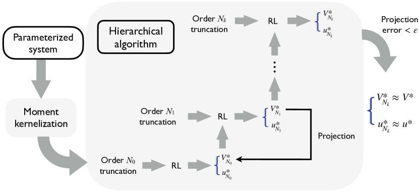
Figure 2: Workflow of the proposed filtrated reinforcement learning for parameterized ensemble systems defined on infinite-dimensional function spaces.

To build the filtrated RL structure for a parameterized system, we observe that for any $N\in\mathbb{N}$, the order $N$ truncated moment system contains any truncated moment system with a lower truncation order $N^{\prime}<N$ as a subsystem. As a result, an RL problem of the order $N^{\prime}$ truncated moment system is a subproblem of that of the order $N$ truncated moment system, which gives rise to a filtrated RL structure along the increasing sequence of truncation orders $N_{0}<N_{1}<\cdots$. Specifically, starting from the moment truncation order $N_{0}$, the optimal policy $u^{*}_{N_{0}}(t)$ and the value function $\widehat{V}_{N_{0}}^{*}(t,\widehat{m}_{N_{0}}(t))$ can be learned for the corresponding truncated moment system. Next, we increase the truncation order to $N_{1}$ to learn $u^{*}_{N_{1}}(t)$ and $\widehat{V}_{N_{1}}^{*}\big{(}t,\widehat{m}_{N_{1}}(t)\big{)}$. Repeating this procedure then generates sequences of control policies $\big{(}u_{N_{k}}^{*}(t)\big{)}_{k\in\mathbb{N}}$ and values functions $\big{(}\widehat{V}^{*}(t,\widehat{m}_{N_{k}}(t))\big{)}_{k\in\mathbb{N}}$. Guaranteed by the moment convergence proved in Theorem 8, the sequence $\big{(}\widehat{V}^{*}(t,\widehat{m}_{N_{k}}(t))\big{)}_{k\in\mathbb{N}}$ necessarily converges to the value function $V^{*}(t,m(t))$ of the entire moment system. Therefore, when the projection error $\sup_{t\in[0,T]}\big{|}\widehat{V}^{*}_{N_{k}}\big{(}t,\widehat{m}^{*}_{N_{k}}(t)\big{)}-\widehat{V}^{*}_{N_{k-1}}\big{(}t,\widehat{m}^{*}_{N_{k-1}}(t)\big{)}\big{|}<\varepsilon$ is satisfied for the prescribed tolerance $\varepsilon>0$, the optimal policy $u_{N_{k}}^{*}(t)$ of the order $N_{k}$ truncated moment system gives an accurate approximation to that $u^{*}(t)$ of the entire moment system, equivalently the original ensemble system. The workflow of this filtrated RL algorithm is shown in Figure 2.

Remark 10 (Optimality preserving filtration)

A reminiscence of the observation made above Theorem 7, that is, $\widehat{V}_{N}^{*}\geq V^{*}|_{\widehat{M}_{N}}$ for any moment truncation order $N\in\mathbb{N}$, directly extends to $\widehat{V}_{N_{i}}^{*}\geq\widehat{V}_{N_{j}}^{*}|_{\widehat{M}_{N_{i}}}\geq\widehat{V}_{N_{j}}^{*}$ for any $i<j$. This means that the optimal policy learned from one hierarchy of the filtrated RL problem is also optimal for, actually may even decrease the values of the cumulative rewards learned from, all the lower-level hierarchies. This demonstrates that the filtrated structure preserves the optimality of each hierarchy in the filtration.

A comparison between the truncated and entire moment systems in (9) and (7) reveals that they are controlled by the same policy, which announces policy search algorithms as the prime candidates for learning the optimal policy. In addition, the optimiality preserving property of the filtrated RL structure mentioned in Remark 10 points out a specific algorithmic approach: the policy learned from the current hierarchy always promises to be a good initial condition for the successive hierarchy, which is shown in Algorithm 1.

Algorithm 1 Filtrated policy search for learning optimal policies for parameterized systems

Parameterized system: initial state $x_{0}$, vector field $F$, final time $T$;

2:  Cumulative reward: immediate reward function $r$, terminal cost $K$;

  Design criterion: projection error tolerance $\varepsilon$

4:Optimal policy $u^{*}$

Initialization: truncation order $N_{0}$, initial policy $u^{(0)}$, projection error $P$, hierarchy level $i=0$

6:while $P>\varepsilon$ do

     if $i>0$ then

8:         $i\leftarrow i+1$

         Pick $N_{i}>N_{i-1}$ and $u^{(0)}\leftarrow u_{N_{i-1}}^{*}$

10:     end if

     Compute order $N_{i}$ truncated moment kernelization: $\widehat{m}_{N_{i}}(0)$, $\widehat{F}_{N_{i}}$, $\bar{r}$, $\bar{K}$

12:     Solve $u_{N_{i}}^{*}(t)={\rm argmin}_{u}\widehat{V}_{N_{i}}(t,\widehat{m}_{N_{i}}(t))$ and compute $\widehat{V}^{*}_{N_{i}}(t,\widehat{m}^{*}_{N_{i}}(t))=\min_{u}\widehat{V}^{*}_{N_{i}}(t,\widehat{m}_{N_{i}}(t))$

     Compute $P=\sup_{t\in[0,T]}\big{|}\widehat{V}^{*}_{N_{i}}\big{(}t,\widehat{m}^{*}_{N_{i}}(t)\big{)}-\widehat{V}^{*}_{N_{i-1}}\big{(}t,\widehat{m}^{*}_{N_{i-1}}(t)\big{)}\big{|}$ with $\widehat{V}^{*}_{N_{-1}}\equiv 0$

14:end while

$u^{*}\leftarrow u^{*}_{N_{i}}$ return $u^{*}$

4.1.1 Spectral sequence convergence of early stopped policy search

Gradient-based methods are the most popular policy search approaches in RL to learn optimal policies, e.g., to solve $u_{N_{i}}^{*}(t)={\rm argmin}_{u}\widehat{V}_{N_{i}}(t,\widehat{m}_{N_{i}}(t))$ in each hierarchy of Algorithm 1. The main idea is to generate a policy sequence in the form of $u_{N_{i}}^{(j)}=u_{N_{i}}^{(j-1)}+\delta u_{N_{i}}^{(j-1)}$ such that $u_{N_{i}}^{(j)}\rightarrow u_{N_{i}}^{*}$ depends on the gradient of $\widehat{V}_{N_{i}}$ with respect to the policy $u_{N_{i}}$ evaluated at $u_{N_{i}}^{(j)}$, where $\delta u^{(j-1)}$. Applying a policy gradient (PG) algorithm to learn $u_{N_{i}}^{*}$ for each $i$ yields the following spectral sequence,

$$\begin{array}[]{ccccccc}&\text{PG iteration }0&\text{PG iteration }1&\cdots&\text{PG iteration }j&\cdots\\ \text{Hierarchy 0}&\widehat{V}_{N_{0}}(t,\widehat{m}^{(0)}_{N_{0}}(t))&\widehat{V}_{N_{0}}(t,\widehat{m}^{(1)}_{N_{0}}(t))&\cdots&\widehat{V}_{N_{0}}(t,\widehat{m}^{(j)}_{N_{0}}(t))&\longrightarrow&\widehat{V}_{N_{0}}^{*}(t,\widehat{m}_{N_{0}}(t))\\ \text{Hierarchy 1}&\widehat{V}_{N_{1}}(t,\widehat{m}^{(0)}_{N_{1}}(t))&\widehat{V}_{N_{1}}(t,\widehat{m}^{(1)}_{N_{1}}(t))&\cdots&\widehat{V}_{N_{1}}(t,\widehat{m}^{(j)}_{N_{1}}(t))&\longrightarrow&\widehat{V}_{N_{1}}^{*}(t,\widehat{m}_{N_{1}}(t))\\ \vdots&\vdots&\vdots&&\vdots&&\vdots\\ \text{Hierarchy $i$}&\widehat{V}_{N_{i}}(t,\widehat{m}^{(0)}_{N_{i}}(t))&\widehat{V}_{N_{i}}(t,\widehat{m}^{(1)}_{N_{i}}(t))&\cdots&\widehat{V}_{N_{i}}(t,\widehat{m}^{(j)}_{N_{i}}(t))&\longrightarrow&\widehat{V}_{N_{i}}^{*}(t,\widehat{m}_{N_{i}}(t))\\ \vdots&\downarrow&\downarrow&&\downarrow&&\downarrow\\ &V(t,m^{(0)}(t))&V(t,m^{(1)}(t))&\cdots&V(t,m^{(j)}(t))&\longrightarrow&V^{*}(t,m(t))\end{array}$$

in which the $i^{\rm th}$ row converges to the value function $\widehat{V}^{*}(t,\widehat{m}_{N_{i}}(t))$ of the order $N_{i}$ truncated moment system and the $j^{\rm th}$ column converges to the cumulative reward $V(t,m^{(j)}(t))$ of the entire moment system. In particular, the row convergence naturally follows from the convergence of gradient methods and the column convergence is a result of the continuity of the cumulative reward function and the convergence of the truncated moment sequence to the entire moment sequence.

Interpreted by using the spectral sequence above, Algorithm 1 is to learn the optimal policy “along the rightmost column”, meaning the learning sequence for the optimal policy of the entire moment system constitutes the optimal policies of all the truncated moment systems. In fact, due to the convergence of both the rows and columns in the spectral sequence, any path towards the “bottom right” generates a learning sequence converging to the optimal policy of the entire moment system, as a direct consequence of Cantor’s diagonal argument (Rudin, 1976). Algorithmically, learning sequences generated by paths other than the rightmost column consists of policies obtained by early stopping the PG algorithm in some hierarchies. For example, in the extreme case, along the diagonal, the learning sequence is generated by evolving only one iteration of the PG algorithm in each hierarchy. In practice, motiviated by “clipped” PG algorithms, e.g., Proximal Policy Optimization (PPO) and Rrust Region Policy Optimization (TRPO), (Schulman et al., 2017, 2015), a natural choice of the early stopping criterion, for starting the next hierarchy of FRL, is a threshold for the variation of the cumulative reward. To be more specific, let $u_{N_{k}}^{(i)}$ be the policy resulting from the $i^{\rm th}$ iteration of the PG algorithm in the $k^{\rm th}$ hierarchy and $\widehat{m}_{N_{k}}^{(i)}$ be the trajectory of the order-$N_{k}$ truncated moment system steered by $u_{N_{k}}^{(i)}$, then we terminate this hierarchy if $\sup_{t\in[0,T]}\big{|}\widehat{V}_{N_{k}}(t,\widehat{m}_{k}^{(i)}(t))-\widehat{V}_{N_{k}}(t,\widehat{m}_{k}^{(i)}(t))\big{|}>\delta$ for the predetermined threshold $\delta>0$. It is also worth mentioning that, different from PPO and TRPO, the threshold is set to evaluate the variation of the cumulative reward, instead of the policy. This choice is made based on the moment convergence properties proved in Theorems 7 and 8 as well as Corollary 9 that both the optimal trajectories and value functions of truncated moment systems converge to those of the entire moment system but the corresponding optimal policies may fail to converge as pointed out at the end of Section 2. In the following, we will propose a second-order policy search algorithm for continuous-time dynamical systems, regardless of the system dimension, and hence can be integrated into the FRL structure.

4.1.2 Second-order policy search

The development of the policy search algorithm is based on the theory of differential dynamic programming (Jacobson and Mayne, 1970; Mayne, 1966), and as a major advantage, the algorithm does not involve time discretization and is directly applicable to infinite-dimensional continuous-time systems, e.g., the moment system in (7). The main idea is to expand the value function into a Taylor series up to the second-order and then derive the update rule in terms of differential equations. In the following, we only highlight the key steps in the development of the algorithm (see Appendix C for the detailed derivation).

Quadratic approximation of Hamilton-Jacobi-Bellman equations.

The Taylor expansion of the value function $V^{*}:\mathbb{R}\times\mathcal{M}\rightarrow\mathbb{R}$ of the moment system is enabled by the inner product on $\mathcal{M}$. Specifically, for any variation $\delta m\in\mathcal{M}$ at $m\in\mathcal{M}$, we have $V^{*}(t,m+\delta m)=V^{*}(t,m)+\langle DV^{*}(t,m),\delta m\rangle+\frac{1}{2}\langle D^{2}V^{*}(t,m)\cdot\delta m,\delta m\rangle+o(\delta m^{2})$, where $D^{2}V^{*}(t,m)$ is identified with a bounded linear operator from $\mathcal{M}\rightarrow\mathcal{M}$ and $D^{2}V^{*}(t,m)\cdot\delta m$ denotes the evaluation of $D^{2}V^{*}(t,m)$ at $\delta m$ (Lang, 1999). The quadratic approximation of the HJB equation in (11) is obtained by replacing $V^{*}$ by its Taylor expansion with the high-order term $o(\delta m^{2})$ neglected, yielding

$$\frac{\partial}{\partial t} V^{*}(t,m)+\Big{\langle}\frac{\partial}{\partial t}DV^{*}(t,m),\delta m\Big{\rangle}+\frac{1}{2}\Big{\langle}\frac{\partial}{\partial t}D^{2}V^{*}(t,m)\cdot\delta m,\delta m\Big{\rangle}$$

$$+\min_{u}\Big{\{}H(t,m+\delta m,u,DV^{*}(t,m))+\Big{\langle}D^{2}V^{*}(t,m)\cdot\delta m,\bar{F}(t,m+\delta m,u)\Big{\rangle}\Big{\}}=0,$$ (15)

where $H(t,m+\delta m,u,DV^{*}(t,m))=\bar{r}(t,m,u)+\langle DV^{*}(t,m),\bar{F}(t,m,u)\rangle$ is the Hamiltonian of the moment system.

Second-order policy search.

The next step is to design an iterative algorithm to solve (15). In particular, the algorithm is used to generate a sequence of policies $u^{(k)}$ by the learning rule $u^{(k+1)}=u^{(k)}+\delta u^{(k)}$ so that $u^{*}=\lim_{k\rightarrow\infty}u^{(k)}$ and $m^{*}=\lim_{k\rightarrow\infty}m^{(k)}$ and the pair $(m^{*},u^{*})$ solves (15), where $m^{(k)}$ and $m^{*}$ are the trajectories of the moment system steered by $u^{(k)}$ and $u^{*}$, respectively. To find $\delta u^{(k)}$, we note that because the pair $(m^{(k)},u^{(k)})$ satisfies the moment system in (7), $\delta m^{(k)}=0$ holds so that the equation in (15) reduces to $\frac{\partial}{\partial t}V^{*}(t,m^{(k)})+\min_{u}H(t,m^{(k)},u,DV(t,m^{(k)}))=0$, in which the solution $\tilde{u}^{(k)}$ of the minimization is represented in terms of $m^{(k)}$ and $DV^{*}(t,m^{(k)})$. Steered by this policy $\tilde{u}^{(k)}$, the trajectory of the moment system is not $m^{(k)}$ any more, and hence a variation $\delta m^{(k)}$ on $m^{(k)}$ is produced so that $m^{(k)}+\delta m^{(k)}$ satisfies the moment system, which also updates the equation in (15) to

$$\frac{\partial}{\partial t} V^{*}(t,m^{(k)})+\Big{\langle}\frac{\partial}{\partial t}DV^{*}(t,m^{(k)}),\delta m^{(k)}\Big{\rangle}+\frac{1}{2}\Big{\langle}\frac{\partial}{\partial t}D^{2}V^{*}(t,m^{(k)})\cdot\delta m^{(k)},\delta m^{(k)}\Big{\rangle}$$

$$\qquad\qquad\qquad\quad+\min_{\delta u}\Big{\{}H(t,m^{(k)}+\delta m^{(k)},\tilde{u}^{(k)}+\delta u,DV^{*}(t,m^{(k)}))$$

$$\qquad\qquad\qquad\qquad+\Big{\langle}D^{2}V^{*}(t,m^{(k)})\cdot\delta m^{(k)},\bar{F}(t,m^{(k)}+\delta m^{(k)},\tilde{u}^{(k)}+\delta u)\Big{\rangle}\Big{\}}=0.$$ (16)

To solve the minimization problem in (16), we expand the objective function into the Taylor series with respect to ($\delta m^{(k)},\delta u$) up to the second-order and then compute the critical point $\delta u^{(k)}$, represented in terms of $DV^{*}(t,m^{(k)})$ and $D^{2}V^{*}(t,m^{(k)})$ as well. Therefore, it remains to find $DV^{*}(t,m^{(k)})$ and $D^{2}V^{*}(t,m^{(k)})$. To this end, we observe that, after the above Taylor expansion, the equation in (16) becomes an algebraic second-order polynomial equation in $\delta m^{(k)}$, which is satisfied if all the coefficients are 0. This yields

$$\frac{d}{dt}\delta V(t,m^{(k)}(t)) =H(t,m^{(k)},{u^{(k)}},DV^{*}(t,m^{(k}))-H(t,m^{(k)},\tilde{u}^{(k)},DV^{*}(t,m^{(k)})),$$ (17)

$$\frac{d}{dt}DV^{*}(t,m^{(k)}(t)) =-DH-D^{2}V\cdot(\bar{F}-\bar{F}(t,m^{(k)},{u^{(k)}})),$$ (18)

$$\frac{d}{dt}D^{2}V^{*}(t,m^{(k)}(t)) =-D^{2}H-D\bar{F}^{\prime}\cdot D^{2}V^{*}-D^{2}{V^{*}}^{\prime}\cdot D\bar{F}$$

$$\,+\left[\frac{\partial DH}{\partial u}+\frac{\partial\bar{F}^{\prime}}{\partial u}\cdot D^{2}V^{*}\right]^{\prime}\cdot\Big{(}\frac{\partial^{2}H}{\partial u^{2}}\Big{)}^{-1}\cdot\left[\frac{\partial DH}{\partial u}+\frac{\partial\bar{F}^{\prime}}{\partial u}\cdot D^{2}V^{*}\right]$$ (19)

with the terminal conditions $DV^{*}(T,m^{(k)}(T))=D\bar{K}(T,m^{(k)}(T))$ and $D^{2}V^{*}(T,m^{(k)}(T))=D\bar{K}(T,m^{(k)}(T))$, where $\delta V(t,m^{(k)}(t))=V^{*}(t,m^{(k)}(t))-V(t,m^{(k)}(t))$ and $V(t,m^{(k)}(t))$ is the cumulative reward of the moment system driven by the policy $u^{(k)}$. Moreover, to simplify the notations, all the functions in the equations in (18) and (19) without arguments are evaluated at $(t,m^{(k)},\tilde{u}^{(k)})$, and ‘$\prime$’ denotes the transpose of linear operators.

Early stopping criterion.

Because the development of the policy search algorithm is built up on the Taylor series approximation, it is required that the amplitudes of $\delta m^{(k)}$ and $\delta u^{(k)}$ are small enough for all $k$. A necessary condition to guarantee this is to bound $\delta V^{(k)}=\sup_{t}|\delta V(t,m^{(k)}(t))|$ by a threshold $\eta$, as a consequence of Assumption C2. When integrating the proposed second-order policy search algorithm into the FRL structure, e.g., at the $i^{\rm th}$ hierarchy, we will start the next hierarchy with the initial policy $u^{(k)}$ by terminating the current one if $\sup_{t}|\widehat{V}_{N_{i}}(t,\widehat{m}_{N_{i}}^{(k)}(t))-\widehat{V}_{N_{i}}(t,\widehat{m}_{N_{i}}^{(k-1)}(t))|>\eta$. The FRL with the early stopped second-order policy search is shown in Algorithm 2.

Algorithm 2 Filtrated reinforcement learning for parameterized systems with the early stopped second-order policy search

Parameterized system: initial state $x_{0}$, vector field $F$, final time $T$

2:  Cumulative reward: immediate reward function $r$, terminal cost $K$

  Design criteria: projection error tolerance $\varepsilon$, value function variation tolerance $\eta$,

4:  maximum iterations of policy search $K$

Optimal ensemble control policy $u^{*}$

6:Initialization: truncation order $N_{0}$, control policy $u^{(0)}$, projection error $P>\varepsilon$, value function variation $\delta V=0$, hierarchy level $i=0$, policy search iteration number $j=0$

while $P>\varepsilon$ do

8:     Compute the order $N_{i}$ truncated moment system in (9)

     while $\delta V\leq\eta$ and $j\leq K$ do

10:         Compute $\widehat{m}_{N_{i}}^{(j)}(t)$ for $0\leq t\leq T$ by applying $u^{(j)}$ to the system in (9)

         Compute $\delta\widehat{V}_{N_{i}}(t,\widehat{m}_{N_{i}}^{(j)}(t))$ $D\widehat{V}_{N_{i}}^{*}(t,\widehat{m}_{N_{i}}^{(j)}(t))$ and $D^{2}\widehat{V}_{N_{i}}^{*}(t,\widehat{m}_{N_{i}}^{(j)}(t))$ for $0\leq t\leq T$ by solving the system of differential equations in (17), (18) and (19)

12:         ${u^{(j+1)}}(t)\leftarrow{\rm argmin}_{a}H(t,\widehat{m}_{N_{i}}^{(j)},a,D\widehat{V}_{N_{i}}(t,\widehat{m}_{N_{i}}^{(j)}))$ for all $0\leq t\leq T$

         $\delta V\leftarrow\max_{t}|\delta\widehat{V}(t,\widehat{m}^{(j)}_{N_{i}})|$

14:         $j\leftarrow j+1$

     end while

16:     $\widehat{m}_{N_{i}}^{*}\leftarrow\widehat{m}_{N_{i}}^{(j-1)}$

     if $i\geq 1$ then

18:         $P=\max_{t\in[0,T]}\big{|}\widehat{V}_{N_{i}}(t,\widehat{m}_{N_{i}}^{*}(t))-\widehat{V}_{N_{i-1}}(t,\widehat{m}_{N_{i-1}}^{*}(t))\big{|}$

     end if

20:     $N_{i+1}\leftarrow N_{i}+1$, $u^{(0)}\leftarrow u^{(j-1)}$

     $i\leftarrow i+1$

22:end while

$u^{*}\leftarrow u^{(j-1)}$ return $u^{*}$

4.2 Examples and simulations

In this section, we will demonstrate the applicability and efficiency of the proposed FRL algorithm by using both linear and nonlinear parameterized systems.

4.2.1 Infinite-dimensional linear–quadratic regulators

Linear-quadratic (LQ) problems, those are, linear systems with cumulative rewards given by quadratic functions, are the most fundamental control problems, which have been well studied for finite-dimensional linear systems (Brockett, 2015; Kwakernaak and Sivan, 1972; Sontag, 1998). However, for parameterized systems defined on infinite-dimensional function spaces, such problems remain barely understood. In this example, we will fill in this literature gap to approach infinite-dimensional LQ problems over function spaces by using the proposed FRL algorithms.

To illuminate the main idea as well as to demonstrate how FRL addresses the curse of dimensionality, we revisit the scalar linear parameterized system in (2), i.e. $\frac{d}{dt}x(t,\beta)=\beta x(t,\beta)+u(t)$, $\beta\in[-1,1]$, with the cumulative reward given by $V(t,x_{t})=\int_{-1}^{1}\Big{[}\int_{t}^{T}\big{(}x^{2}(t,\beta)+u^{2}(t)\big{)}dtd\beta+x^{2}(T,\beta)\Big{]}d\beta$. To apply the moment kernel transform, we evolve the system on the Hilbert space $L^{2}(\Omega)$, consisting of square-integrable real-valued functions defined on $\Omega$, and then choose the basis $\{\Phi_{k}\}_{k\in\mathbb{N}}$, as in the definition of moments in (5), to be the set of Chebyshev polynomials. Then, the moment kernelized system and cumulative reward are given by $\frac{d}{dt}m(t)=Am(t)+bu(t)$ and $V(t,m(t))=\int_{0}^{T}\big{[}\|m(t)\|^{2}+2u^{2}(t)\big{]}dt+\|m(T)\|^{2}$, where $A=\frac{1}{2}(L+R)$ with $L$ and $R$ the left- and right-shift operators, given by $(m_{0}(t),m_{1}(t),\dots)\mapsto(m_{1}(t),m_{2}(t),\dots)$ and $(m_{0}(t),m_{1}(t),\dots)\mapsto(0,m_{0}(t),\dots)$, respectively (see Appendix D.1 for the detailed derivation).

We then apply Algorithm 2 to learn the finite-time horizon LQR policy for the parameterized linear system in (2). In the simulation, we choose the final time and initial condition for the parameterized system to be $T=1$ and $x_{0}=1$, the constant function on $[-1,1]$, respectively, the tolerance for the value function variation to be $\eta=1$, and vary the truncation order $N$ from $2$ to $10$, and the simulation results are illustrated in Figure 3. Specifically, Figure 3(a) shows the total cumulative reward $\widehat{V}(0,\widehat{m}_{N}(0))$ (top panel) and the number of the policy search iterations (bottom panel) with respect to the truncation order (hierarchy level) $N$. In particular, we observe that the total cumulative reward converges to the minimum cost in only 4 hierarchies of the algorithm, which demonstrates the high efficiency of FRL. Correspondingly, Figure 3(b) plots the policy $u_{N}$ learned from each hierarchy of FRL, which stabilizes to the shadowed region starting from $N=6$. In addition, it is worth mentioning that the computational time for running 10 hierarchies of the algorithm is only 3.97 second, indicating the low computational cost of the algorithm. As a result, the curse of dimensionality is effectively mitigated.

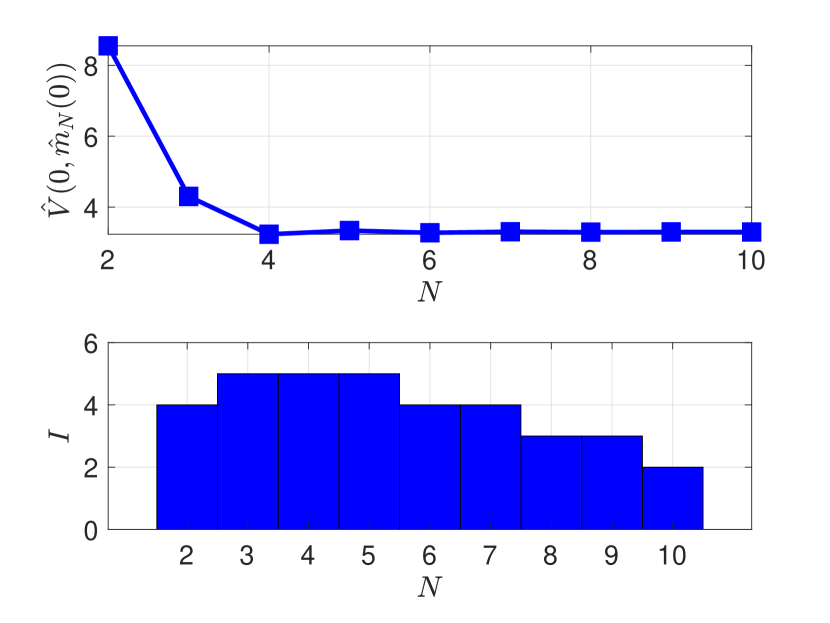
(a)

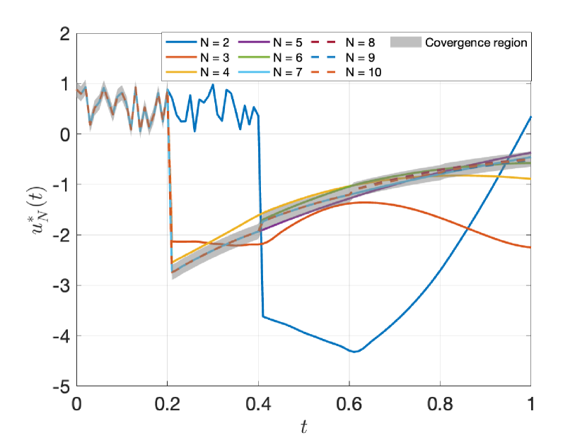
(b)

Figure 3: Learning the finite-time horizon LQR policy for the parameterized system in (2) by using Algorithm 2. In particular, (a) shows the total cumulative reward (top panel) and the number of the policy search iterations with respect to the truncation order (hierarchy level) $N$ ranging from 2 to 20, and (b) plots the learned policy from each hierarchy of FRL.

To further demonstrate the advantages of FRL, in addition to the mitigation of the curse of dimensionality, we will show that it also resolves the convergence issue caused by applying classical RL algorithms to sampled parameterized systems as pointed out in Section 2.1. To this end, we revisit the infinite-time horizon LQR problem presented there, that is, the same system in (2) as above with the cumulative reward given by $V(x_{t})=\int_{-1}^{1}\int_{0}^{\infty}e^{-2.5t}\big{[}x^{2}(t,\beta)+u^{2}(t)\big{]}dtd\beta$. In this case, we use Algorithm 1 with the standard value iteration applied to each hierarchy, and the simulation results are shown in Figure 4. A comparison between Figures 4(a) and 1(b) reveals that now the difference between the value functions and optimal policies learned from successive hierarchies of FRL converge to 0. Meaning, the sequences of value functions and optimal policies generated by Algorithm 1 are Cauchy sequences, and hence necessarily converge to those of the parameterized system in (2) (Rudin, 1976). To be more specific, as shown in Figure 4(b), the learned value functions and optimal policies stabilize to the corresponding shadowed regions.

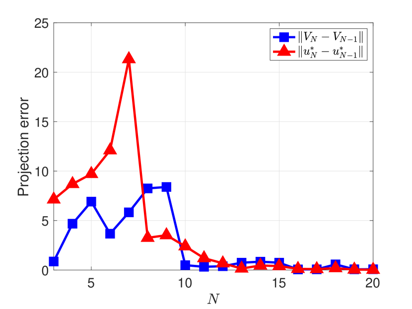
(a)

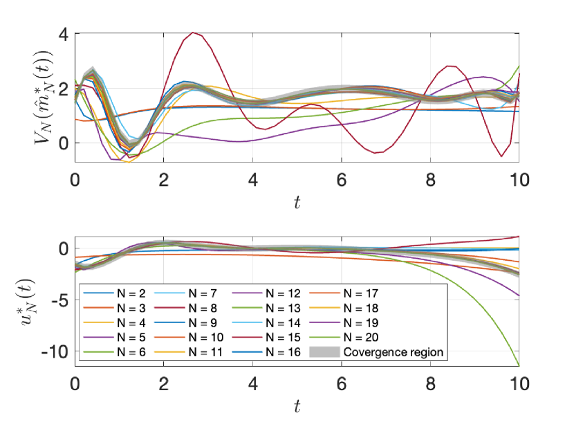
(b)

Figure 4: FRL resolves the convergence issue caused by applying classical RL algorithms to sampled parameterized systems. In particular, Algorithm 1 with the value iteration applied to each hierarchy is used to learn the infinite-time horizon LQR value function and policy of the parameterized system in (2). Specifically, (a) plots the error between the value functions and optimal policies learned from successive hierachies, and (b) shows the learned value function (top) optimal policy (bottom) in each hierarchy.

4.2.2 Filtrated reinforcement learning for nonlinear population systems

Robust excitation of a nuclear spin sample, typically consisting of as many as spins in the order of the Avogadro’s number ($\sim 10^{23}$), is a crucial problem in quantum science and technology. For example, it enables all the applications of nuclear magnetic resonance (NMR) spectroscopy, including magnetic resonance imaging (MRI), quantum computing, quantum optics, and quantum information processing (Li and Khaneja, 2009; Li et al., 2022; Silver et al., 1985; Roos and Moelmer, 2004; Stefanatos and Li, 2011; Chen et al., 2011; Stefanatos and Li, 2014). The dynamics of nuclear spins (immersed in a static magnetic field with respect to the rotating frame) is governed by the Bloch equation

$$\frac{d}{dt}x(t,\beta)=\left[\begin{array}[]{ccc}0&0&-\beta u(t)\\ 0&0&\beta v(t)\\ \beta u(t)&-\beta v(t)&0\end{array}\right]x(t,\beta)$$ (23)

derived by the Swiss-American physicist Felix Bloch in 1946 (Cavanagh et al., 2010). In this system, the state variable $x(t,\beta)$ denotes the bulk magnetization, $u(t)$ and $v(t)$ represent the external radio frequency (rf) fields, and the system parameter $\beta\in\Omega=[1-\delta,1+\delta]$ with $0<\delta<1$ is referred to as the rf inhomogeneity, characterizing the phenomenon that spins in different positions of the sample receive different strength of the rf fields. In practice, the difference can be up to $\delta=40\%$ of the strength of the applied rf fields (Nishimura et al., 2001). A typical policy learning task is to design the rf fields $u(t)$ and $v(t)$, with the minimum energy, to steer the parameterized Bloch system in (23) from the equilibrium state $x_{0}(\beta)=(0,0,1)^{\prime}$ to the excited state $x_{F}(\beta)=(1,0,0)^{\prime}$ for all $\beta$. We formulate this policy design task as an RL problem over $L^{2}(\Omega,\mathbb{R}^{3})$, i.e., $x(t,\cdot)\in L^{2}(\Omega,\mathbb{R}^{3})$, with the cumulative reward $V(t,x_{t})=\int_{t}^{T}\big{(}u^{2}(t)+v^{2}(t)\big{)}dt+\int_{1-\delta}^{1+\delta}|x(T,\beta)-x_{F}(\beta)|^{2}d\beta$, where $|\cdot|$ denotes a norm on $\mathbb{R}^{3}$.

We still use the Chebyshev polynomial basis $\{\Phi_{k}\}_{k\in\mathbb{N}}$ to kernelize the Bloch system and the cumulative reward. To guarantee the orthonomality of $\{\Phi_{k}\}_{k\in\mathbb{N}}$, we first rescale the range of the rf inhomogenity from $[1-\delta,1+\delta]$ to $[-1,1]$ by the linear transformation $\beta\mapsto\eta=(\beta-1)/\delta$, and then apply the moment kernel transform defined in (5). This yields the moment kernelized system and cumulatvive reward given by $\frac{d}{dt}m(t)=\Big{[}\frac{\delta}{2}(R+L)+I\Big{]}\otimes\big{[}u(t)\Omega_{y}+v(t)\Omega_{x}\big{]}m(t)$ and $V(t,m(t))=\int_{t}^{T}\big{(}u^{2}(t)+v^{2}(t)\big{)}dt+\|m(T)-m_{F}\|^{2}$, respectively, where $\Omega_{x}=\left[\begin{array}[]{ccc}0&0&0\\ 0&0&1\\ 0&-1&0\end{array}\right]$ and $\Omega_{y}=\left[\begin{array}[]{ccc}0&0&-1\\ 0&0&0\\ 1&0&0\end{array}\right]$, $I$ denotes the identity operator for real-valued sequences and $\otimes$ is the tensor product of linear operators (see Appendix D.2).

We then apply Algorithm 2 to learn the optimal policies for the spin system in (23) with rf inhomogeneity. In the simulation, we consider the maximal rf inhomogeneity $\delta=40\%$ in practice and pick the final time to be $T=1$, and the results are shown in Figure 5. Specifically, Figure 5(a) shows the total cumulative reward (top panel) and number of policy search iterations (bottom panel) with respect to the moment truncation order $N$, that is, the hierarchy level as well, from which we observe the convergence of the algorithm at $N=9$. Figure 5(b) plots the policies learned from each hierarchy, which stabilize to the corresponding shadowed regions eventually. The computational time is 53.33 seconds, which is much longer than that (3.97 seconds) for the LQR problem presented in Section 4.2.1. This is because the order-$N$ truncated moment system in this case is of dimension $3N$, 3 times higher than the moment system in the LQR case. In addition, the nonlinearity of the Bloch system also increase the complexity of this policy learning task.

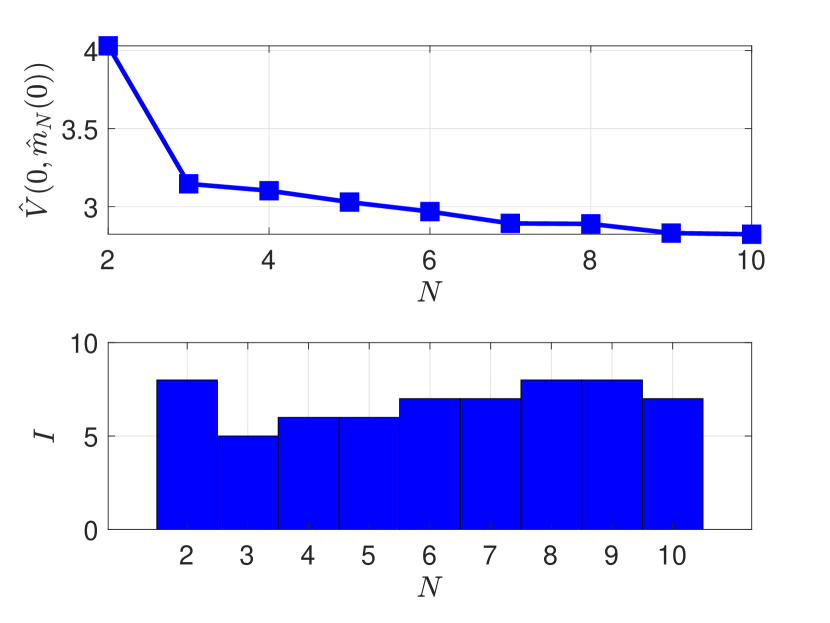
(a)

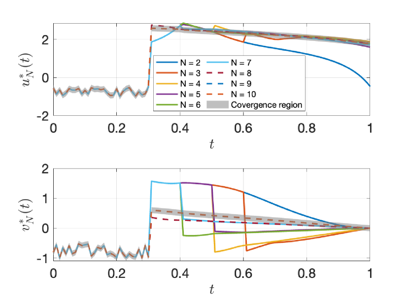
(b)

Figure 5: Policy learning for the nuclear spin system in (23) under rf inhomogeneity by using Algorithm 2. In particular, (a) shows the total cumulative reward (top panel) and number of the policy search iterations with respect to the moment truncation order, that is, the hierarchy level, $N$ ranging from 2 to 10, and (b) plots the policies learned from each hierarchy of the algorithm.

As mentioned previously, from the perspective of quantum physics, a goal of controlling the Bloch system is to steer the spins from the equilibrium state $(0,0,1)^{\prime}$ to the excited state $(1,0,0)^{\prime}$ uniformly regardless of the rf inhomogeneity. Note that because $\Omega_{x}$ and $\Omega_{y}$ are skew-symmetric matrices, $|x(t,\beta)|=1$ holds for all $t$ and $\beta$, to evaluate the excitation performance, it suffices to examine $x_{1}(T,\beta)$, the first component of the final state $x(T,\beta)$, which is plotted in the top panel of Figure 6(a) as a function of $\beta$. Specifically, its average value, generally used as the measure of the control performance (Zhang and Li, 2015), is $\frac{1}{2\delta}\int_{1-\delta}^{1+\delta}x_{1}(T,\beta)d\beta=0.9613$, which is close to 1, showing the good performance of the learned policies. The bottom panel of Figure 6(a) shows the performance measure versus time. Moreover, Figure 6(b) shows the entire trajectory of the Bloch system on the unit sphere, from which we observe that the learned policies indeed steer the system towards the excited state $(1,0,0)^{\prime}$, regardless of the rf inhomogeneity, as desired.

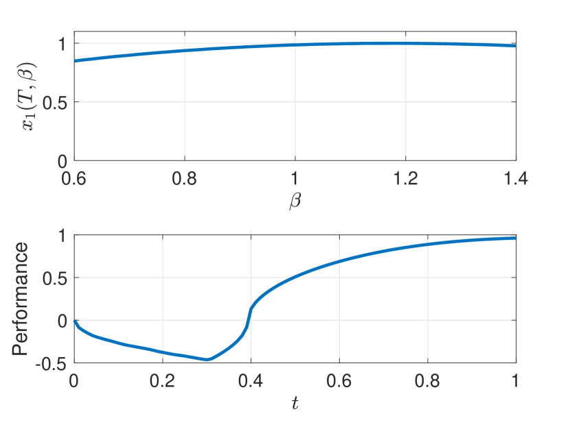
(a)

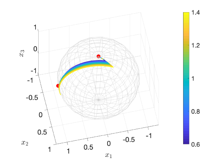
(b)

Figure 6: Excitation performance of the policies learned by using Algorithm 2. In particular, (a) plots the first component of the final state of the Bloch system in (23) with respect to the rf inhomogeneity $\beta$, and (b) shows the entire trajectory of the system driven by the learned policies.

5 Conclusion

In this paper, we propose a novel reinforcement learning architecture for learning optimal policies to shape the collective dynamic behavior of populations of intelligent agents of arbitrarily large population sizes. In particular, we formulate such a population as a parameterized deterministic control system defined on an infinite-dimensional function space, which leads to an functional setting for reinforcement learning of the infinite-dimensional system. To mitigate the challenges arising from the infinite-dimensionality, we develop the moment kernel transform carrying over the system and its value function to a reproducing kernel Hilbert space consisting of moment sequences, giving rise to a kernel parameterization of the reinforcement learning problem. We then utilize this moment kernelization to develop a hierarchical policy learning algorithm with a convergence guarantee, where each hierarchy is composed of a reinforcement learning problem for a finite-dimensional truncated moment kernelized system. We further investigate early stopping criteria for each hierarchy to improve the computational efficiency of the algorithm, and prove the convergence of the early stopped algorithm in terms of spectral sequences. Moreover, examples are provided for demonstration of the excellent performance and high efficiency of the proposed algorithm.

The presented FRL architecture, although showcased in the model-based setting, is directly applicable in the data-driven environment. In this case, for instance, the equations in (17), (18), and (19), involved in Algorithm 2, can be represented by neural ordinary differential equations. Our next step is to explore data-driven FRL and also generalize it to large-scale populations of intelligent agents placed in stochastic environments, e.g., those with the dynamics described by stochastic differential equations.

Acknowledgments and Disclosure of Funding

This work was supported by the Air Force Office of Scientific Research under the award FA9550-21-1-0335.

Appendix A Proof of Lemma 2

Let $x_{k}(t,\cdot)$ and $x(t,\cdot)$ in $\mathcal{F}(\Omega,M)$ be the trajectories (solutions) of the ensemble system in (3), with the initial condition $x(0,\cdot)$, driven by the control inputs $u_{k}$ and $u$, respectively, for all $k\in\mathbb{N}$, i.e.,

$$\frac{d}{dt}x_{k}(t,\beta)=F\big{(}t,\beta,x_{k}(t,\beta),u_{k}(t)\big{)}\quad\text{and}\quad\frac{d}{dt}x(t,\beta)=F\big{(}t,\beta,x(t,\beta),u(t)\big{)}.$$

We claim that $x_{k}(t,\cdot)$ converges to $x(t,\cdot)$ on $\mathcal{F}(\Omega,M)$ pointwisely as $k\rightarrow\infty$ for any $t\in[0,T]$, which is equivalent to $x_{k}(t,\beta)\rightarrow x(t,\beta)$ for any $\beta\in\Omega$ on each coordinate chart of $M$ by using a partition of unity on $M$ (Lee, 2012). Therefore, it suffices to assume that the entire trajectories $x_{k}([0,T],\beta)\subseteq M$ and $x([0,T],\beta)\subseteq M$ for all $k\in\mathbb{N}$ and each $\beta\in\Omega$ are located in a single coordinate chart of $M$ and hence equivalently in $\mathbb{R}^{n}$.

To prove the claim, we fix an arbitrary $\beta\in\Omega$ and note that

$$\frac{d}{dt}\Big{(}x_{k}(t,\beta)-x(t,\beta)\Big{)} =F\big{(}t,\beta,x_{k}(t,\beta),u_{k}(t))-F(t,\beta,x(t,\beta),u(t)\big{)}$$

$$\leq\Big{|}F\big{(}t,\beta,x_{k}(t,\beta),u_{k}(t))-F(t,\beta,x(t,\beta),u(t)\big{)}\Big{|}$$

$$\leq\Big{|}F\big{(}t,\beta,x_{k}(t,\beta),u_{k}(t)\big{)}-F\big{(}t,\beta,x(t,\beta),u_{k}(t)\big{)}\Big{|}$$

$$\qquad\qquad+\Big{|}F\big{(}t,\beta,x(t,\beta),u_{k}(t)\big{)}-F\big{(}t,\beta,x(t,\beta),u(t)\big{)}\Big{|},$$

where the second inequality follows from the triangle inequality. Because $\frac{d}{dt}\big{(}x(t,\beta)-x_{k}(t,\beta)\big{)}$ satisfies the same inequality as above, we obtain

$$\frac{d}{dt}\Big{|}x_{k}(t,\beta)-x(t,\beta)\Big{|} \leq\Big{|}F\big{(}t,\beta,x_{k}(t,\beta),u_{k}(t)\big{)}-F\big{(}t,\beta,x(t,\beta),u_{k}(t)\big{)}\Big{|}$$

$$\qquad\qquad+\Big{|}F\big{(}t,\beta,x(t,\beta),u_{k}(t)\big{)}-F\big{(}t,\beta,x(t,\beta),u(t)\big{)}\Big{|}$$

$$\leq C\Big{|}x_{k}(t,\beta)-x(t,\beta)\Big{|}+\Big{|}F\big{(}t,\beta,x(t,\beta),u_{k}(t)\big{)}-F\big{(}t,\beta,x(t,\beta),u(t)\big{)}\Big{|}$$

where the second inequality follows from the Lipschitz continuity of $F$ in the system state variable according to Assumption S2. Moreover, as solutions of ordinary differential equations, all of $x_{k}(t,\beta)$ and $x(t,\beta)$ are Lipschitz continuous, and hence absolutely continuous, then so is $|x_{k}(t,\beta)-x(t,\beta)|$. Together with its nonnegativity, Gronwall’s inequality can be applied (Evans, 2010), yielding

$$\Big{|}x_{k}(t,\beta)-x(t,\beta)\Big{|}\leq e^{Ct}\int_{0}^{t}\Big{|}F\big{(}s,\beta,x(s,\beta),u_{k}(s)\big{)}-F\big{(}s,\beta,x(s,\beta),u(s)\big{)}\Big{|}ds$$

Because $F$ is continuous in the control policy variable, the pointwise convergence of $u_{k}(s)$ to $u(s)$ implies that of $F\big{(}s,\beta,x(s,\beta),u_{k}(s)\big{)}$ to $F\big{(}s,\beta,x(s,\beta),u(s)\big{)}$. Then, by Egoroff’s Theorem, there exist sequences of real numbers $\varepsilon_{k}>0$ and subsets $I_{k}$ of $[0,T]$ with Lebesgue measure $\varepsilon_{k}$ such that $\varepsilon_{k}\rightarrow 0$ and $F\big{(}s,\beta,x(s,\beta),u_{k}(s)\big{)}\rightarrow F\big{(}s,\beta,x(s,\beta),u(s)\big{)}$ uniformly on $I_{k}^{c}=[0,T]\backslash I_{k}$. Consequently, we have

$$\lim_{k\rightarrow\infty} \Big{|}x_{k}(t,\beta)-x(t,\beta)\Big{|}\leq\lim_{k\rightarrow\infty}e^{Ct}\int_{0}^{t}\Big{|}F\big{(}s,\beta,x(s,\beta),u_{k}(s)\big{)}-F\big{(}s,\beta,x(s,\beta),u(s)\big{)}\Big{|}ds$$

$$\leq e^{Ct}\Big{\{}\lim_{k\rightarrow\infty}\int_{I_{k}^{c}}\Big{|}F\big{(}s,\beta,x(s,\beta),u_{k}(s)\big{)}-F\big{(}s,\beta,x(s,\beta),u(s)\big{)}\Big{|}ds$$

$$\qquad\qquad\qquad+\lim_{k\rightarrow\infty}\int_{I_{k}}\Big{|}F\big{(}s,\beta,x(s,\beta),u_{k}(s)\big{)}-F\big{(}s,\beta,x(s,\beta),u(s)\big{)}\Big{|}ds\Big{\}}$$

$$=e^{Ct}\Big{\{}\int_{0}^{t}\lim_{k\rightarrow\infty}\Big{|}F\big{(}s,\beta,x(s,\beta),u_{k}(s)\big{)}-F\big{(}s,\beta,x(s,\beta),u(s)\big{)}\Big{|}\chi_{I_{k}^{c}}(s)ds$$

$$\qquad\qquad\qquad+\lim_{k\rightarrow\infty}\int_{I_{k}}\Big{|}F\big{(}s,\beta,x(s,\beta),u_{k}(s)\big{)}-F\big{(}s,\beta,x(s,\beta),u(s)\big{)}\Big{|}ds\Big{\}}=0,$$

in which $\chi_{I_{k}^{c}}$ denotes the characteristic function of $I_{k}^{c}$, i.e., $\chi_{I_{k}^{c}}(s)=1$ for $s\in I_{k}^{c}$ and $\chi_{I_{k}^{c}}(s)=0$ for $s\not\in I_{k}^{c}$, the change of the limit and integral in the first term in the summand follows from the uniform convergence of $F\big{(}s,\beta,x(s,\beta),u_{k}(s)\big{)}$ to $F\big{(}s,\beta,x(s,\beta),u(s)\big{)}$ on $I_{k}^{c}$, and the second integral converges 0 because the Lebesgue of $I_{k}$ goes to 0. This then proves the claim.

Now, without loss of generality, we assume that $|J(u)|<\infty$, and the existence of such a $u$ is guaranteed by Assumption C1. Then, we obtain the desired convergence

$$\lim_{k\rightarrow\infty}J(u_{k}) =\lim_{k\rightarrow\infty}\Big{[}\int_{\Omega}\int_{0}^{T}r(t,x_{k}(t,\beta),u_{k}(t))dtd\beta+\int_{\Omega}K(T,x_{k}(T,\beta))d\beta\Big{]}$$

$$=\int_{\Omega}\int_{0}^{T}\lim_{k\rightarrow\infty}r(x_{k}(t,\beta),u_{k}(t))dtd\beta+\int_{\Omega}\lim_{k\rightarrow\infty}K(x_{k}(T,\beta))d\beta$$

$$=\int_{\Omega}\int_{0}^{T}r(t,\lim_{k\rightarrow\infty}x_{k}(t,\beta),\lim_{k\rightarrow\infty}u_{k}(t))dtd\beta+\int_{\Omega}K(T,\lim_{k\rightarrow\infty}x_{k}(T,\beta))d\beta$$

$$=\int_{\Omega}\int_{0}^{T}r(t,x(t,\beta),u(t))dtd\beta+\int_{\Omega}K(T,x(T,\beta))d\beta=J(u),$$

where the second and third equalities follow from the dominated convergence theorem and the continuity of $r$ and $K$, respectively (Folland, 2013).

Appendix B Proof of Proposition 6

Fix $z,\tilde{z}\in\mathcal{M}$ and $t,\tilde{t}\in[0,T]$, then by the definition of the infimum, for any $\varepsilon>0$, there exists an ensemble control policy $u\in\mathcal{U}$ such that

$$V^{*}(\tilde{t},\tilde{z})+\varepsilon \geq\int_{\tilde{t}}^{T}\bar{r}(\tau,\tilde{m}(\tau),u(\tau))d\tau+\bar{K}(T,\tilde{m}(T))$$

$$=\int_{\Omega}\int_{\tilde{t}}^{T}r(\tau,\tilde{x}(\tau,\beta),u(\tau))d\tau d\beta+\int_{\Omega}K(T,\tilde{x}(T,\beta))d\beta,$$

where $\tilde{m}(\tau)$ satisfies the moment system $\frac{d}{d\tau}\tilde{m}(\tau)=\bar{F}(\tau,\tilde{m}(\tau),u(\tau))$ with the initial condition $\tilde{m}(s)=\tilde{z}$ and $\tilde{x}(t,\cdot)$ is the trajectory of the associated ensmeble system. Next, let $m(\tau)$ be the trajectory of the moment system steered by the same control policy with the initial condition $m(t)=z$ and $x(t,\cdot)$ be the associated ensemble trajectory. Without loss of generality, we assume that $t\leq\tilde{t}$, and then we have

$$V^{*}(t,z)-V^{*}(\tilde{t},\tilde{z}) \leq\int_{\Omega}\int_{t}^{T}r(\tau,x(\tau,\beta),u(\tau))d\tau d\beta+\int_{\Omega}K(T,x(T,\beta))d\beta$$

$$\qquad\quad-\int_{\Omega}\int_{\tilde{t}}^{T}r(\tau,\tilde{x}(\tau,\beta),u(\tau))d\tau d\beta-\int_{\Omega}K(T,\tilde{x}(T,\beta))d\beta+\varepsilon$$

$$=\int_{\Omega}\int_{t}^{\tilde{t}}r(\tau,x(\tau,\beta),u(\tau))d\tau d\beta+\int_{\Omega}\int_{\tilde{t}}^{T}\Big{[}r(\tau,x(\tau,\beta),u(\tau))$$

$$\quad\ -r(\tau,\tilde{x}(\tau,\beta),u(\tau))\Big{]}d\tau d\beta+\int_{\Omega}\Big{[}K(T,x(T,\beta))-K(T,\tilde{x}(T,\beta))\Big{]}d\beta+\varepsilon.$$ (24)

Because finite-time solutions of ordinary differential equations with initial conditions in a bounded set remain bounded, $|r(\tau,x(\tau,\beta),u(\tau))|\leq M$ holds for some $M$ over $\tau\in[t,\tilde{t}]$ so that the first term in (24) can be bounded as

$$\int_{\Omega}\int_{t}^{\tilde{t}}r(\tau,x(\tau,\beta),u(\tau))d\tau d\beta\leq\int_{\Omega}\int_{t}^{\tilde{t}}|r(\tau,x(\tau,\beta),u(\tau))|d\tau d\beta M\leq{\rm Vol}(\Omega)|t-\tilde{t}|.$$

Then, by using the Lipschtiz continuity of $r$ and $K$ as in Assumption C2, the second and third terms in (24) satisfies

$$\int_{\Omega}\int_{\tilde{t}}^{T} \Big{[}r(\tau,x(\tau,\beta),u(\tau))-r(\tau,\tilde{x}(\tau,\beta),u(\tau))\Big{]}d\tau d\beta+\int_{\Omega}\Big{[}K(T,x(T,\beta))-K(T,\tilde{x}(T,\beta))\Big{]}d\beta$$

$$\leq\int_{\Omega}\int_{\tilde{t}}^{T}C_{r}\big{|}x(\tau,\beta)-\tilde{x}(\tau,\beta)\big{|}d\tau d\beta+\int_{\Omega}C_{K}\big{|}x(T,\beta)-\tilde{x}(T,\beta)\big{|}d\beta$$

$$\leq\int_{\Omega}(TC_{r}+C_{K})C^{\prime}\big{|}x(\tilde{t},\beta)-\tilde{x}(\tilde{t},\beta)\big{|}d\beta$$

$$\leq(TC_{r}+C_{K})C^{\prime}\int_{\Omega}\Big{[}\big{|}x(t,\beta)-\tilde{x}(\tilde{t},\beta)\big{|}+\big{|}x(t,\beta)-x(\tilde{t},\beta)\big{|}\Big{]}d\beta$$

$$\leq(TC_{r}+C_{K})C^{\prime}\Big{[}\int_{\Omega}\big{|}x(t,\beta)-\tilde{x}(\tilde{t},\beta)\big{|}d\beta+\int_{\Omega}\big{|}x(t,\beta)-x(\tilde{t},\beta)\big{|}d\beta\Big{]},$$ (25)

where the second inequality follows from Gronwall’s inequality. Note that the first integral in (25) is exactly the $L^{1}$-norm of $x(t,\cdot)-\tilde{x}(t,\cdot)$, which is equal to $\|z-\tilde{z}\|$, the norm of the associated moment sequences, since the moment transformation is an isometry. For the second term, we use the Lipschitz continuity of solutions to ordinary differential equations to conclude $\int_{\Omega}\big{|}x(t,\beta)-x(\tilde{t},\beta)\big{|}\leq C^{\prime\prime}{\rm Vol}(\Omega)|t-\tilde{t}|$ for some $C^{\prime\prime}>0$. Now, let $C=\max\{(TC_{r}+C_{K})C^{\prime},M{\rm Vol}(\Omega),{\rm Vol}(\Omega)\}$, then we obtain $V^{*}(t,z)-V^{*}(\tilde{t},\tilde{z})\leq C(|t-\tilde{t}|+\|z-\tilde{z}\|)$ since $\varepsilon>0$ is arbitrary. The same argument with the roles of $(t,z)$ and $(\tilde{t},\tilde{z})$ reversed implies

$$|V^{*}(t,z)-V^{*}(\tilde{t},\tilde{z})|\leq C(|t-\tilde{t}|+\|z-\tilde{z}\|),$$

giving the Lipschitz continuity of $V^{*}$ on $[0,T]\times\mathcal{M}$ as desired.

Appendix C Derivation of Second-Order Policy Search Update Equations

Quadratic approximation of Hamilton-Jacobi-Bellman equations.

We pick a nominal policy $\bar{u}(t)$, which generates a nominal trajectory $\bar{m}(t)$ by applying $\bar{u}(t)$ to the moment system in (7). Then, the optimal policy and trajectory can be represented as $u^{*}(t)=\bar{u}(t)+\delta u(t)$ and $m^{*}(t)=\bar{m}(t)+\delta m(t)$, respectively, plugging which into the Hamiltonian-Jacobi-Bellman equation in (11), i.e.,

$$\frac{\partial}{\partial t}V(t,z)+\min_{a\in U}\big{\{}\bar{r}(t,z,a)+\langle DV(t,z),\bar{F}(t,z,a)\rangle\big{\}}=0$$

yields

$$\frac{\partial}{\partial t}V(t,\bar{m}+\delta m)+\min_{\delta u}\big{\{} \bar{r}(t,\bar{m}+\delta m,\bar{u}+\delta u)$$

$$+\langle DV(t,\bar{m}+\delta m),\bar{F}(t,\bar{m}+\delta m,\bar{u}+\delta u)\rangle\big{\}}=0,$$

where, and in the following as well, we drop the time argument $t$ from the state and control variables for the conciseness of the representation. Now, we assume that the value function $V:[0,T]\times\mathcal{M}\rightarrow\mathbb{R}$ is smooth enough, at least in the region containing the nominal and optimal trajectories, to admit a second-order power series expansion as

$$V(t, \bar{m}+\delta m)=V(t,\bar{m})+\langle DV(t,\bar{m}),\delta m\rangle+\frac{1}{2}\langle D^{2}V(t,\bar{m})\cdot\delta m,\delta m\rangle+o(\delta m^{2})$$

$$=\bar{V}(t,\bar{m})+\delta V(t,\bar{m})+\langle DV(t,\bar{m}),\delta m\rangle+\frac{1}{2}\langle D^{2}V(t,\bar{m})\cdot\delta m,\delta m\rangle+o(\delta m^{2}),$$ (26)

where we further expand $V(t,\bar{m})$ by using the nominal cost $\bar{V}(t,\bar{m})=\int_{t}^{T}\bar{r}(s,\bar{m}(s),\bar{u}(s))ds+K(T,\bar{m}(T))$, that is, the cost obtained by applying the nominal control input $\bar{u}$ to the system starting from $\bar{m}(t)$ at time $t$. To explain the second-order term in the above expansion, by the definition, the second derivative $D^{2}V(t,\bar{m})$ of the real-valued function $V(t,\cdot):\mathcal{M}\rightarrow\mathbb{R}$ evaluated at $\bar{m}$ is a bounded linear map from $\mathcal{M}$ to $\mathcal{M}^{*}$ (Lang, 1999). In our notation, $D^{2}V(t,\bar{m})\cdot\delta m$ denotes the evaluation of $D^{2}V(t,\bar{m})$ at $\delta m$, giving an element in $\mathcal{M}^{*}$ that can be paired with $\delta m\in\mathcal{M}$. Conceptually, $D^{2}V(t,\bar{m})$ is nothing but the infinite-dimensional Hessian matrix with the $(i,j)$-entry given by $\frac{\partial^{2}V}{\partial z_{i}\partial z_{j}}|_{(t,\bar{m})}$. If $\delta m$ is small enough to ensure a sufficiently accurate approximation of the value function $V(t,\bar{m})$ up to the second-order terms, then we integrate (26) with the $o(\delta m^{2})$ term neglected into the Hamilton-Jacobi-Bellman equation, yielding

$$\frac{\partial}{\partial t} \bar{V}(t,\bar{m})+\frac{\partial}{\partial t}\delta V(t,\bar{m})+\Big{\langle}\frac{\partial}{\partial t}DV(t,\bar{m}),\delta m\Big{\rangle}+\frac{1}{2}\Big{\langle}\frac{\partial}{\partial t}D^{2}V(t,\bar{m})\cdot\delta m,\delta m\Big{\rangle}$$

$$+\min_{\delta u}\Big{\{}H(t,\bar{m}+\delta m,\bar{u}+\delta u,DV(t,\bar{m}))+\Big{\langle}D^{2}V(t,\bar{m})\cdot\delta m,\bar{F}(t,\bar{m}+\delta m,\bar{u}+\delta u)\Big{\rangle}\Big{\}}=0$$ (27)

with the system Hamiltonian $H(t,m,u,DV)=\bar{r}(t,m,u)+\langle DV(t,m),\bar{F}(t,m,u)\rangle$, which is the key equation to the development of the algorithm for successively improving the nominal control policy $\bar{u}$.

Second-order policy search.

To initialize the algorithm, we start with a nominal control policy $u_{0}$, applying which to the moment system generates a nominal trajectory $m^{(0)}$. Because the pair $(m^{(0)},u^{(0)})$ satisfies the system, the variation of the trajectory is $\delta m=0$. In this case, the second-order expanded Hamilton-Jacobi-Bellman equation in (27) takes the form

$$\frac{\partial}{\partial t}\bar{V}(t,m^{(0)})+\frac{\partial}{\partial t}\delta V(t,m^{(0)})+\min_{\delta u}H(t,m^{(0)},u^{(0)}+\delta u,DV(t,m^{(0)}))=0,$$ (28)

and in many cases, the minimization of the Hamiltonian can be solved analytically, giving a new control policy ${u^{(0)}}^{*}$, represented in terms of $m^{(0)}$ and $DV(t,m^{(0)})$ as a feedback control. However, steered by this policy, the system trajectory may not be the nominal one anymore, and hence a variation $\delta m$ is introduced to the nominal trajectory as $m^{(0)}+\delta m$. Correspondingly, the second-order expanded Hamilton-Jacobi-Bellman equation becomes the one in (27) with $\bar{u}$ replaced by ${u^{(0)}}^{*}$, in which the minimization is taken over $\delta u$ for the function

$$H(t,m^{(0)}+\delta m,{u^{(0)}}^{*}+\delta u,DV(t,m^{(0)}))+\Big{\langle}D^{2}V(t,m^{(0)})\cdot\delta m,\bar{F}(t,m^{(0)}+\delta m,{u^{(0)}}^{*}+\delta u)\Big{\rangle}.$$

We further expand this function around $(m^{(0)},{u^{(0)}}^{*})$ up to the second-order terms, yielding

$$H+\Big{\langle}\frac{\partial H}{\partial u}, \delta u\Big{\rangle}+\Big{\langle}DH+D^{2}V\cdot\bar{F},\delta m\Big{\rangle}+\Big{\langle}\Big{(}\frac{\partial DH}{\partial u}+\frac{\partial\bar{F}^{\prime}}{\partial u}\cdot D^{2}V\Big{)}\cdot\delta m,\delta u\Big{\rangle}$$

$$+\frac{1}{2}\Big{\langle}\frac{\partial^{2}H}{\partial u^{2}}\cdot\delta u,\delta u\Big{\rangle}+\frac{1}{2}\Big{\langle}\Big{(}D^{2}H+D\bar{F}^{\prime}\cdot D^{2}V+D^{2}V^{\prime}\cdot DF\Big{)}\cdot\delta m,\delta m\Big{\rangle},$$ (29)

where the terms involving $H$, $\bar{F}$, and $V$ are evaluated at $(t,m^{(0)},{u^{(0)}}^{*},DV(t,m^{(0)}))$, $(t,m^{(0)}$, ${u^{(0)}}^{*})$, and $(t,m^{(0)})$, respectively, and ‘$\prime$’ denotes the dual of a linear operator. For example, because $\bar{F}(t,m^{0},u_{0}^{*})\in\mathcal{M}$ by identifying the tangent space of $\mathcal{M}$ at $m^{0}$ with $\mathcal{M}$ itself, $D\bar{F}(t,m^{(0)},{u^{(0)}}^{*}):\mathcal{M}\rightarrow\mathcal{M}$ is a linear map, then its dual operator is defined as a linear map $D\bar{F}^{\prime}(t,m^{0},u_{0}^{*}):\mathcal{M}^{*}\rightarrow\mathcal{M}^{*}$ satisfying $\langle L,D\bar{F}(t,m^{(0)},{u^{(0)}}^{*})\cdot z\rangle=\langle D\bar{F}^{\prime}(t,m^{(0)},{u^{(0)}}^{*})\cdot L,z\rangle$ for any $z\in\mathcal{M}$ and $L\in\mathcal{M}^{*}$ (Yosida, 1980). Conceptually, dual operators are nothing but transpose matrices. Next, to minimize the function in (29), the necessary condition is the vanishing of its derivative with respect to $\delta u$, giving

$$\frac{\partial H}{\partial u}+\frac{\partial^{2}H}{\partial u^{2}}\cdot\delta u+\Big{(}\frac{\partial DH}{\partial u}+\frac{\partial\bar{F}^{\prime}}{\partial u}\cdot D^{2}V\Big{)}\cdot\delta m=0,$$ (30)

in which it is necessary that $\frac{\partial H}{\partial u}|_{(t,m^{(0)},{u^{(0)}}^{*},DV(t,m^{(0)}))}=0$ since $u$ minimizes the Hamiltonian $H(t,m^{(0)},{u^{(0)}}^{*},DV(t,m^{(0)}))$ by our choice.

Recall that our intention is to approximate the Hamiton-Jacobi-Bellman equation up to the second-order term in $\delta m$. Therefore, it is required that $\delta m$ and $\delta u$ are in the same order, meaning, they satisfy a linear relationship; otherwise, say $\delta u$ is quadratic in $\delta m$, then the terms $\Big{\langle}\Big{(}\frac{\partial DH}{\partial u}+\frac{\partial\bar{F}^{\prime}}{\partial u}\cdot D^{2}V\Big{)}\cdot\delta m,\delta u\Big{\rangle}$ and $\frac{1}{2}\Big{\langle}\frac{\partial^{2}H}{\partial u^{2}}\cdot\delta u,\delta u\Big{\rangle}$ in (29) are of orders higher than $\delta m^{2}$. Formally, there is a linear map $A:\mathcal{M}\rightarrow\mathbb{R}^{m}$ such that $\delta u=A\cdot\delta m$. To find $A$, we replace $\delta u$ by $A\cdot\delta m$ in the necessary optimality condition in (30), leading to

$$A=-\left(\frac{\partial^{2}H}{\partial u^{2}}\right)^{-1}\cdot\Big{(}\frac{\partial DH}{\partial u}+\frac{\partial\bar{F}^{\prime}}{\partial u}\cdot D^{2}V\Big{)}.$$

With this choice of $A$, the function in (29) becomes

$$H+\Big{\langle}DH+ D^{2}V\cdot\bar{F},\delta m\Big{\rangle}$$

$$+\frac{1}{2}\Big{\langle}\Big{(}D^{2}H+D\bar{F}^{\prime}\cdot D^{2}V+D^{2}V^{\prime}\cdot DF-A^{\prime}\cdot D^{2}H\cdot A\Big{)}\cdot\delta m,\delta m\Big{\rangle}$$

so that the second-order expansion of the Hamilton-Jacobi-Bellman equation in (27) takes the form

$$\frac{\partial}{\partial t}\bar{V}+\frac{\partial}{\partial t} \delta V+\Big{\langle}\frac{\partial}{\partial t}DV,\delta m\Big{\rangle}+\frac{1}{2}\Big{\langle}\frac{\partial}{\partial t}D^{2}V(t,\bar{m})\cdot\delta m,\delta m\Big{\rangle}+H+\Big{\langle}DH+D^{2}V\cdot\bar{F},\delta m\Big{\rangle}$$

$$+\frac{1}{2}\Big{\langle}\Big{(}D^{2}H+D\bar{F}^{\prime}\cdot D^{2}V+D^{2}V^{\prime}\cdot DF-A^{\prime}\cdot\frac{\partial^{2}H}{\partial u^{2}}\cdot A\Big{)}\cdot\delta m,\delta m\Big{\rangle}=0,$$ (31)

Because $\delta m$ is arbitrary, the coefficient of each order of $\delta m$ must be 0, which transforms (31) into a system of three partial differential equations

$$\frac{\partial}{\partial t}\bar{V}+\frac{\partial}{\partial t}\delta V-H=0$$

$$\frac{\partial}{\partial t}DV-DH-D^{2}V\cdot\bar{F}=0$$

$$\frac{\partial}{\partial t}D^{2}V-D^{2}H-D\bar{F}^{\prime}\cdot D^{2}V-D^{2}V^{\prime}\cdot DF+A^{\prime}\cdot\frac{\partial^{2}H}{\partial u^{2}}H\cdot A=0$$

with terms involving $H$, $\bar{F}$, and $V$ are evaluated at $(t,m^{(0)},{u^{(0)}}^{*},DV(t,m^{(0)}))$, $(t,m^{(0)},{u^{(0)}}^{*})$, and $(t,m^{(0)})$, respectively, as before. Integrating with the chain rule as

$$\frac{d}{dt}(\bar{V}+\delta V)=\frac{\partial}{\partial t}\bar{V}+\frac{\partial}{\partial t}\delta V+\big{\langle}DV,\bar{F}(t,m^{(0)},{u^{(0)}})\big{\rangle}$$

$$\frac{d}{dt}DV=\frac{\partial}{\partial t}DV+D^{2}V\cdot\bar{F}(t,m^{(0)},{u^{(0)}})$$

$$\frac{d}{dt}D^{2}V=\frac{\partial}{\partial t}D^{2}V+\frac{1}{2}D^{3}V\cdot\bar{F}(t,m^{(0)},{u^{(0)}})+\frac{1}{2}\bar{F}(t,m^{(0)},{u^{(0)}})^{\prime}\cdot D^{3}V^{\prime}$$

then gives three ordinary differential equations

$$\frac{d}{dt}\delta V(t,m^{(0)}(t)) =H(t,m^{(0)},{u^{(0)}},DV(t,m^{(0)}))-H(t,m^{(0)},{u^{(0)}}^{*},DV(t,m^{(0)})),$$ (32)

$$\frac{d}{dt}DV(t,m^{(0)}(t)) =-DH-D^{2}V\cdot(\bar{F}(t,m^{(0)},{u^{(0)}}^{*})-\bar{F}(t,m^{(0)},{u^{(0)}})),$$ (33)

$$\frac{d}{dt}D^{2}V(t,m^{(0)}(t)) =-D^{2}H-D\bar{F}^{\prime}\cdot D^{2}V-D^{2}V^{\prime}\cdot D\bar{F}$$

$$\qquad\quad+\left[\frac{\partial DH}{\partial u}+\frac{\partial\bar{F}^{\prime}}{\partial u}\cdot D^{2}V\right]^{\prime}\cdot\Big{(}\frac{\partial^{2}H}{\partial u^{2}}\Big{)}^{-1}\cdot\left[\frac{\partial DH}{\partial u}+\frac{\partial\bar{F}^{\prime}}{\partial u}\cdot D^{2}V\right],$$ (34)

where we use $\frac{d}{dt}\bar{V}(t,m^{(0)}(t))=\frac{d}{dt}\big{\{}\int_{t}^{T}\bar{r}(s,m^{(0)}(s),u^{(0)}(s))ds+\bar{K}(T,m^{(0)}(T))\big{\}}=-\bar{r}(t$, $m^{(0)}(s),u^{(0)}(s))$ and $A=-\left(\frac{\partial^{2}H}{\partial u^{2}}\right)^{-1}\cdot\Big{(}\frac{\partial DH}{\partial u}+\frac{\partial\bar{F}^{\prime}}{\partial u}\cdot D^{2}V\Big{)}$, and omit the third-order terms involving $D^{3}V$. Moreover, because the value function satisfies $V(T,m^{(0)}(T))=\bar{K}(T,m^{(0)}(T))$, we have the terminal conditions for the ordinary differential equations in (32) to (33) as $\delta V(T,m^{(0)}(T))=0$, $DV(T,m^{(0)}(T))=D\bar{K}(T,m^{(0)}(T))$, and $D^{2}V(T,m^{(0)}(T))=D^{2}\bar{K}(T,m^{(0)}(T))$. In particular, the data $DV(t,m^{(0)}(t))$ obtained from solving the above systems of differential equations is then used to compute the control policy ${u^{(0)}}^{*}$, which has been represented in terms of $\bar{m}(t)$ and $DV(t,m^{(0)}(t))$ when minimizing the Hamitonian in (28) and hence gives rise to an improvement of the nominal control policy $u^{(0)}$. This in turn completes one iteration of the proposed policy search algorithm.

Appendix D Derivation of Moment Systems

D.1 Infinite-dimensional LQR

In the following, we consider the finite-time horizion LQR problem

$$\begin{cases}\frac{d}{dt}x(t,\beta)=\beta x(t,\beta)+u(t),\\ V(t,x_{t})=\int_{\Omega}\Big{[}\int_{0}^{T}\big{(}x^{2}(t,\beta)+u^{2}(t)\big{)}dtd\beta+x^{2}(T,\beta)\Big{]}d\beta,\end{cases}$$ (35)

where $\Omega=[-1,1]$ and $x_{t}\in L^{2}(\Omega)$, the space of real-valued square-integrable functions defined on $\Omega$.

Moment kernelization.

We pick $\{\Phi_{k}\}_{k\in\mathbb{N}}$ to be the set of Chebyshev polynomials, and by using the recursive relation of Chebyshev polynomials $2\Phi_{k}=\Phi_{k-1}+\Phi_{k-1}$, we have

$$\frac{d}{dt}m_{k}(t) =\frac{d}{dt}\int_{-1}^{1}\Phi_{k}(\beta)x(t,\beta)d\beta=\int_{-1}^{1}\Phi_{k}(\beta)\frac{d}{dt}x(t,\beta)d\beta=\int_{-1}^{1}\Phi_{k}(\beta)\big{[}\beta x(t,\beta)+u(t)\big{]}d\beta$$

$$=\frac{1}{2}\int_{-1}^{1}\big{[}\Phi_{k-1}(\beta)+\Phi_{k+1}(\beta)\big{]}x(t,\beta)d\beta+\int_{-1}^{1}\Phi_{k}(\beta)d\beta\cdot u(t)$$

$$=\frac{1}{2}\big{[}m_{k-1}(t)+m_{k+1}(t)\big{]}+b_{k}u(t),$$

where the change of the integral and time derivative follows from the dominant convergence theorem (Folland, 2013), $\Phi_{-1}$, and hence $m_{-1}$, are defined to be identically 0, and $b_{k}$ is given by $\frac{(-1)^{k}+1}{1-k^{2}}$ for $k\neq 1$ and 0 otherwise. We further let $L:\ell^{2}\rightarrow\ell^{2}$ and $R:\ell^{2}\rightarrow\ell^{2}$ denote the left and right shift operators, given by, $(m_{0}(t),m_{1}(t),\dots)\mapsto(m_{1}(t),m_{2}(t),\dots)$ and $(m_{0}(t),m_{1}(t),\dots)\mapsto(0,m_{0}(t),\dots)$, respectively, then the moment system associated with the linear ensemble system in (35) is a linear system evolving on $\ell^{2}$ in the form $\frac{d}{dt}m(t)=Am(t)+Bu(t)$ with $A=\frac{1}{2}(L+R)$ and $B\in\ell^{2}$ whose $k^{\rm th}$ component is $b_{k}$. On the other hand, to parameterize the cost functional, we note that the moment transformation, that is, the Fourier transform, is a unitary operator from $L^{2}(\Omega)$ to $\ell^{2}$, as a result of which $J(u)=\int_{0}^{1}\big{[}\|m(t)\|^{2}+2u^{2}(t)\big{]}dt+\|m(T)\|^{2}$ in the moment parameterization, where $\|\cdot\|$ denotes the $\ell^{2}$ norm. In summary, the LQR problem in (35) in the moment kernel parameterization has the form

$$\begin{cases}\frac{d}{dt}m(t)=Am(t)+Bu(t),\\ V(t,m(T))=\int_{0}^{1}\Big{[}\|m(t)\|^{2}+2u^{2}(t)\Big{]}dt+\|m(T)\|^{2}.\end{cases}$$ (36)

Second-order policy search.

The Hamitonian $H:\ell^{2}\times\mathbb{R}\times\ell^{2}\rightarrow\mathbb{R}$ of the moment system in (36) is given by $(z,a,p)\mapsto\|z\|^{2}+2a^{2}+\langle p,Az+Ba\rangle$, in which $\langle\cdot,\cdot\rangle$ is the $\ell^{2}$ inner product. Let $V:[0,T]\times\ell^{2}\rightarrow\mathbb{R}$ be the value function, then along a trajectory $m(t)$ of the system, by setting $\frac{\partial H}{\partial a}|_{(m(t),a,DV(t,m(t)))}=4a+\langle DV(m(t)),B\rangle=0$, we obtain $u^{*}(t)=-\frac{1}{4}\langle DV(t,m(t)),B\rangle$. Consequently, the differential equations in (32) to (34) for the policy improvement algorithm read

$$\frac{d}{dt}\delta V(t,m(t)) =\Big{[}u+\frac{1}{4}\langle DV,B\rangle\Big{]}^{2},$$

$$\frac{d}{dt}DV(t,m(t)) =-2m-A^{\prime}\cdot DV-D^{2}V\cdot\Big{(}u-\frac{1}{4}\langle DV,B\rangle\Big{)},$$

$$\frac{d}{dt}D^{2}V(t,m(t)) =-2I-A^{\prime}\cdot D^{2}V-D^{2}V\cdot A+\frac{1}{4}D^{2}V\cdot B\cdot B^{\prime}\cdot D^{2}V,$$

where $I$ denotes the identity operator on $\ell^{2}$ and we use the fact that $D^{2}V$ is a self-adjoint operator on $\ell^{2}$. More concretely, when applying Algorithm 2 to a truncated moment system, say of truncation order $N$, then $A$ and $B$ in the above system of differential equations are replaced by

$$\widehat{A}_{N}=\frac{1}{2}\left[\begin{array}[]{ccccc}0&1&&&\\ 1&0&1&&\\ &1&0&\ddots&\\ &&\ddots&\ddots&1\\ &&&1&0\end{array}\right]\in\mathbb{R}^{(N+1)\times(N+1)}\quad\text{and}\quad\widehat{B}_{N}=\left[\begin{array}[]{c}b_{0}\\ b_{1}\\ b_{2}\\ \vdots\\ b_{N}\end{array}\right]\in\mathbb{R}^{N+1},$$

respectively, and the operator dual is essentially the matrix transpose.

D.2 Moment kernelization of nuclear spin systems

The policy learning problem for the nuclear spin systems in (23) is given by

$$\begin{cases}\frac{d}{dt}x(t,\beta)=\beta\big{[}u(t)\Omega_{y}+v(t)\Omega_{x}\big{]}x(t,\beta),\\ V(t,x_{t})=\int_{t}^{T}\big{(}u^{2}(t)+v^{2}(t)\big{)}dt+\int_{1-\delta}^{1+\delta}|x(T,\beta)-x_{F}(\beta)|^{2}d\beta,\end{cases}$$

where the Bloch system is defined on $L^{2}(\Omega,\mathbb{R}^{3})$ with $\Omega=[1-\delta,1+\delta]$ for some $0<\delta<1$.

Moment kernelization.

Similar to the LQR case presented above, we still define the moments by using the set of Chebyshev polynomials $\{\Phi_{k}\}_{k\in\mathbb{N}}$. However, in order to fully utilize the orthonormal property of Chebyshev polynomials, which only holds on $\Omega^{\prime}=[-1,1]$, we consider the transformation $\psi:\Omega\rightarrow\Omega^{\prime}$, given by $\beta\mapsto(\beta-1)/\delta$, and defined the moments by

$$m_{k}(t)=\int_{\Omega}\Phi_{k}\circ\psi\cdot x_{t}d\lambda=\int_{\Omega^{\prime}}\Phi\cdot x_{t}\circ\psi^{-1}d\psi_{\#}\lambda,$$

where $\lambda$ denotes the Lebesgue measure on $\mathbb{R}$, and $\psi_{\#}\lambda$ is the pushforward measure of $\lambda$ by $\psi$, that is, $\psi_{\#}\lambda(I)=\lambda(\psi^{-1}(I))=\delta\lambda(I)$ is satisfied for $I\subseteq\mathbb{R}$, equivalently $d\psi_{\#}\lambda=\delta d\lambda$. This directly implies that the cost functional in the moment parameterization takes the form $J(u,v)=\int_{0}^{T}(u^{2}(t)+v^{2}(t))dt+\|m(T)\|^{2}$, where $\|\cdot\|$ denotes the $\ell^{2}$-norm on the $\mathbb{R}^{3}$-valued sequences, given by, $\|m(T)\|^{2}=\sum_{k=0}^{\infty}|m_{k}(T)|^{2}$. Next, we compute the moment parameterization of the Bloch system in (23) as follows

$$\frac{d}{dt}m_{k}(t) =\frac{d}{dt}\int_{-1}^{1}\Phi_{k}(\eta)\cdot x(t,\psi^{-1}(\eta))d\psi_{\#}\lambda(\eta)=\int_{-1}^{1}\Phi_{k}(\eta)\frac{d}{dt}x(t,\psi^{-1}(\eta))d\psi_{\#}\lambda(\eta)$$

$$=\int_{-1}^{1}\Phi_{k}(\eta)(\delta\eta+1)\big{[}u(t)\Omega_{y}+v(t)\Omega_{x}\big{]}x(t,\psi^{-1}(\eta))d\psi_{\#}\lambda(\eta)$$

$$=\big{[}u(t)\Omega_{y}+v(t)\Omega_{x}\big{]}\cdot\Big{\{}\frac{\delta}{2}\big{[}m_{k-1}(t)+m_{k+1}(t)\big{]}+m_{k}(t)\Big{\}},$$

where we use the recursive relation satisfied by Chebyshev polynomials, i.e., $2\Phi_{k}=\Phi_{k-1}+\Phi_{k+1}$, together with $\Phi_{-1}=0$. Let $L$ and $R$ be the left and right shift operators for real-valued sequences as introduced in Section 4.2.1, the moment parameterization of the Bloch ensemble system is given by $\frac{d}{dt}m(t)=\Big{[}\frac{\delta}{2}(R+L)+I\Big{]}\otimes\big{[}u(t)\Omega_{y}+v(t)\Omega_{x}\big{]}m(t)$, where $I$ denotes the identity operator for real-valued sequences and $\otimes$ be the tensor product of linear operators. As a result, we have obtained the moment kernel parameterization of the RL problem for the Bloch system as

$$\begin{cases}\frac{d}{dt}m(t)=\big{[}u(t)B_{y}+v(t)B_{x}\big{]}m(t),\\ V(t,m(t))=\int_{0}^{T}\big{(}u^{2}(t)+v^{2}(t)\big{)}dt+\|m(T)-m_{F}\|^{2}\end{cases}$$ (37)

where we define $B_{x}=\big{[}\delta(R+L)/2+I\big{]}\otimes\Omega_{x}$ and $B_{y}=\big{[}\delta(R+L)/2+I\big{]}\otimes\Omega_{y}$ to simplify the notations, and $m_{0}$ and $m_{F}$ are the moment sequences of the constant functions $x_{0}(\beta)=(0,0,1)^{\prime}$ and $x_{F}(\beta)=(1,0,0)^{\prime}$, respectively.

Second-order policy search.

The Hamiltonian of the moment system in (37) is given by $H:(\ell^{2})^{3}\times\mathbb{R}\times\mathbb{R}\times(\ell^{2})^{3}\rightarrow\mathbb{R}$, $(z,a,b,p)\mapsto a^{2}+b^{2}+\langle p,\big{[}aB_{y}+bB_{x}\big{]}z\rangle$. Let $V:[0,T]\times\ell^{2}\rightarrow\mathbb{R}$ be the value function, then along a moment trajectory, by setting $\frac{\partial H}{\partial a}|_{(m(t),a,b,DV(t,m(t)))}=2a+\langle DV,B_{y}m(t)\rangle=0$ and $\frac{\partial H}{\partial b}|_{(m(t),a,b,DV(t,m(t)))}=2b+\langle DV,B_{x}m(t)\rangle=0$, we obtain the optimal policies $u^{*}(t)=-\langle DV,B_{y}m(t)\rangle/2$ and $v^{*}(t)=-\langle DV,B_{y}m(t)\rangle/2$. Integrating them into the system of differential equations in (32) to (34) for the policy improvement algorithm yields

$$\frac{d}{dt}\delta V(t,m(t)) =(u-u^{*})^{2}+(v-v^{*})^{2},$$

$$\frac{d}{dt}DV(t,m(t)) =-DV\cdot(u^{*}B_{y}+v^{*}B_{x})-D^{2}V\cdot\big{[}(u^{*}-u)B_{y}+(v^{*}-v)B_{x}\big{]}m,$$

$$\frac{d}{dt}D^{2}V(t,m(t)) =-(u^{*}B_{y}+v^{*}B_{x})^{\prime}\cdot D^{2}V-D^{2}V\cdot(u^{*}B_{y}+v^{*}B_{x}),$$

$$\quad\quad+\frac{1}{2}(DV\cdot B_{y}+m^{\prime}\cdot B_{y}^{\prime}\cdot D^{2}V)^{\prime}\cdot(DV\cdot B_{y}+m^{\prime}\cdot B_{y}^{\prime}\cdot D^{2}V)$$

$$\quad\quad\quad\quad+\frac{1}{2}(DV\cdot B_{x}+m^{\prime}\cdot B_{x}^{\prime}\cdot D^{2}V)^{\prime}\cdot(DV\cdot B_{x}+m^{\prime}\cdot B_{x}^{\prime}\cdot D^{2}V).$$

Specifically, when applying Algorithm 2 to the order $N$ truncated problem, $B_{x}$ and $B_{y}$ are replaced by the $\mathbb{R}^{3(N+1)\times 3(N+1)}$ block matrices

$$(\widehat{B_{x}})_{N}=\frac{1}{2}\left[\begin{array}[]{ccccc}0&\Omega_{x}&&&\\ \Omega_{x}&0&\Omega_{x}&&\\ &\Omega_{x}&0&\ddots&\\ &&\ddots&\ddots&\Omega_{x}\\ &&&\Omega_{x}&0\end{array}\right]\quad\text{ and }\quad(\widehat{B_{y}})_{N}=\frac{1}{2}\left[\begin{array}[]{ccccc}0&\Omega_{y}&&&\\ \Omega_{y}&0&\Omega_{y}&&\\ &\Omega_{y}&0&\ddots&\\ &&\ddots&\ddots&\Omega_{y}\\ &&&\Omega_{y}&0\end{array}\right],$$

respectively.

References

- Albrecht et al. (2024) S.V. Albrecht, F. Christianos, and L. Schäfer. Multi-Agent Reinforcement Learning: Foundations and Modern Approaches. MIT Press, 2024.
- Arnold (1978) Vladimir I. Arnold. Ordinary Differential Equations. MIT Press, 1978.
- Baker et al. (2020) Bowen Baker, Ingmar Kanitscheider, Todor Markov, Yi Wu, Glenn Powell, Bob McGrew, and Igor Mordatch. Emergent tool use from multi-agent autocurricula. In International Conference on Learning Representations, 2020.
- Becker and Bretl (2012) Aaron Becker and Timothy Bretl. Approximate steering of a unicycle under bounded model perturbation using ensemble control. IEEE Transactions on Robotics, 28(3):580–591, 2012.
- Bellemare et al. (2020) Marc G. Bellemare, Salvatore Candido, Pablo Samuel Castro, Jun Gong, Marlos C. Machado, Subhodeep Moitra, Sameera S. Ponda, and Ziyu Wang. Autonomous navigation of stratospheric balloons using reinforcement learning. Nature, 588(7836):77–82, 2020. doi: 10.1038/s41586-020-2939-8. URL https://doi.org/10.1038/s41586-020-2939-8.
- Bellman (1961) R. Bellman. Adaptive Control Processes: A Guided Tour. Princeton Legacy Library. Princeton University Press, 1961.
- Bellman et al. (1957) R. Bellman, Rand Corporation, and Karreman Mathematics Research Collection. Dynamic Programming. Rand Corporation research study. Princeton University Press, 1957.
- Bertsekas and Tsitsiklis (1996) D. Bertsekas and J.N. Tsitsiklis. Neuro-Dynamic Programming. Athena Scientific, 1996.
- Bertsekas (2019) Dimitri Bertsekas. Reinforcement Learning and Optimal Control. Athena Scientific, 2019.
- Brockett (2015) Roger W. Brockett. Finite Dimensional Linear Systems, volume 74 of Classics in Applied Mathematics. Society for Industrial and Applied Mathematics, 2015.
- Bukov et al. (2018) Marin Bukov, Alexandre G. R. Day, Dries Sels, Phillip Weinberg, Anatoli Polkovnikov, and Pankaj Mehta. Reinforcement learning in different phases of quantum control. Phys. Rev. X, 8:031086, Sep 2018.
- Buşoniu et al. (2010) Lucian Buşoniu, Robert Babuška, and Bart De Schutter. Multi-agent Reinforcement Learning: An Overview, pages 183–221. Springer Berlin Heidelberg, Berlin, Heidelberg, 2010.
- Cavanagh et al. (2010) John Cavanagh, Nicholas J. Skelton, Wayne J. Fairbrother, Mark Rance, and III Arthur G. Palmer. Protein NMR Spectroscopy: Principles and Practice. Elsevier, 2 edition, 2010.
- Chen et al. (2014) Chunlin Chen, Daoyi Dong, Ruixing Long, Ian R. Petersen, and Herschel A. Rabitz. Sampling-based learning control of inhomogeneous quantum ensembles. Phys. Rev. A, 89:023402, Feb 2014. doi: 10.1103/PhysRevA.89.023402. URL https://link.aps.org/doi/10.1103/PhysRevA.89.023402.
- Chen et al. (2011) X. Chen, E. Torrontegui, D. Stefanatos, J.-S. Li, and J. G. Muga. Optimal trajectories for efficient atomic transport without final excitation. Physical Review A, 84:043415, 2011.
- Ching and Ritt (2013) ShiNung Ching and Jason T. Ritt. Control strategies for underactuated neural ensembles driven by optogenetic stimulation. Front Neural Circuits, 7:54, 2013.
- Dong et al. (2008) Daoyi Dong, Chunlin Chen, Hanxiong Li, and Tzyh-Jong Tarn. Quantum reinforcement learning. IEEE Transactions on Systems, Man, and Cybernetics, Part B (Cybernetics), 38(5):1207–1220, 2008. doi: 10.1109/TSMCB.2008.925743.
- Evans et al. (2020) Ethan N. Evans, Marcus A. Periera, George I. Boutselis, and Evangelos A. Theodorou. Variational optimization based reinforcement learning for infinite dimensional stochastic systems. In Leslie Pack Kaelbling, Danica Kragic, and Komei Sugiura, editors, Proceedings of the Conference on Robot Learning, volume 100 of Proceedings of Machine Learning Research, pages 1231–1246. PMLR, 30 Oct–01 Nov 2020.
- Evans (2010) Lawrence C. Evans. Partial Differential Equations, volume 19 of Graduate Studies in Mathematics. American Mathematical Society, 2nd edition, 2010.
- Foerster et al. (2016) Jakob Foerster, Ioannis Alexandros Assael, Nando de Freitas, and Shimon Whiteson. Learning to communicate with deep multi-agent reinforcement learning. In D. Lee, M. Sugiyama, U. Luxburg, I. Guyon, and R. Garnett, editors, Advances in Neural Information Processing Systems, volume 29. Curran Associates, Inc., 2016.
- Folland (2013) Gerald B. Folland. Real Analysis: Modern Techniques and Their Applications, volume 40 of Pure and Applied Mathematics: A Wiley Series of Texts, Monographs and Tracts. John Wiley & Sons, 2 edition, 2013.
- François-Lavet et al. (2018) Vincent François-Lavet, Peter Henderson, Riashat Islam, Marc G. Bellemare, and Joelle Pineau. An introduction to deep reinforcement learning. Foundations and Trends® in Machine Learning, 11(3-4):219–354, 2018. ISSN 1935-8237. doi: 10.1561/2200000071.
- Gelada et al. (2019) Carles Gelada, Saurabh Kumar, Jacob Buckman, Ofir Nachum, and Marc G. Bellemare. DeepMDP: Learning continuous latent space models for representation learning. In Kamalika Chaudhuri and Ruslan Salakhutdinov, editors, Proceedings of the 36th International Conference on Machine Learning, volume 97 of Proceedings of Machine Learning Research, pages 2170–2179. PMLR, 09–15 Jun 2019.
- Glaser et al. (1998) S. J. Glaser, T. Schulte-Herbrüggen, M. Sieveking, N. C. Nielsen O. Schedletzky, O. W. Sørensen, and C. Griesinger. Unitary control in quantum ensembles, maximizing signal intensity in coherent spectroscopy. Science, 280:421–424, 1998.
- Gupta et al. (2017) Jayesh K. Gupta, Maxim Egorov, and Mykel Kochenderfer. Cooperative multi-agent control using deep reinforcement learning. In Gita Sukthankar and Juan A. Rodriguez-Aguilar, editors, Autonomous Agents and Multiagent Systems, pages 66–83, Cham, 2017. Springer International Publishing. ISBN 978-3-319-71682-4.
- Hamburger (1920) Hans L. Hamburger. Über eine erweiterung des stieltjesschen momentenproblems. Mathematische Annalen, 82:120–164, 1920.
- Hamburger (1921a) Hans L. Hamburger. Über eine erweiterung des stieltjesschen momentenproblems. Mathematische Annalen, 82:168–187, 1921a.
- Hamburger (1921b) Hans L. Hamburger. Über eine erweiterung des stieltjesschen momentenproblems. Mathematische Annalen, 81:235–319, 1921b.
- Haug et al. (2021) Tobias Haug, Rainer Dumke, Leong-Chuan Kwek, Christian Miniatura, and Luigi Amico. Machine-learning engineering of quantum currents. Phys. Rev. Res., 3:013034, Jan 2021.
- Hausdorff (1923) Felix Hausdorff. Momentprobleme für ein endliches intervall. Mathematische Zeitschrift, 16(1):220–248, 1923.
- Herculano-Houzel (2012) Suzana Herculano-Houzel. The remarkable, yet not extraordinary, human brain as a scaled-up primate brain and its associated cost. Proceedings of the National Academy of Sciences, 109(supplement_1):10661–10668, 2012.
- Heredia et al. (2020) Paulo Heredia, Hasan Ghadialy, and Shaoshuai Mou. Finite-sample analysis of distributed q-learning for multi-agent networks. In 2020 American Control Conference (ACC), pages 3511–3516, 2020.
- Heredia et al. (2022) Paulo Heredia, Jemin George, and Shaoshuai Mou. Distributed offline reinforcement learning. In 2022 IEEE 61st Conference on Decision and Control (CDC), pages 4621–4626, 2022.
- Heredia and Mou (2019) Paulo C. Heredia and Shaoshuai Mou. Distributed multi-agent reinforcement learning by actor-critic method. IFAC-PapersOnLine, 52(20):363–368, 2019. ISSN 2405-8963. doi: https://doi.org/10.1016/j.ifacol.2019.12.182. URL https://www.sciencedirect.com/science/article/pii/S240589631932035X. 8th IFAC Workshop on Distributed Estimation and Control in Networked Systems NECSYS 2019.
- Jacobson and Mayne (1970) David H. Jacobson and David Q. Mayne. Differential Dynamic Programming. Modern Analytic and Computational Mehtods in Sciencen and Mathematics. American Elsevier Publishing Company, 1970.
- Jiang et al. (2021) Wei-Cheng Jiang, Vignesh Narayanan, and Jr-Shin Li. Model learning and knowledge sharing for cooperative multiagent systems in stochastic environment. IEEE Transactions on Cybernetics, 51(12):5717–5727, 2021.
- Kaiser et al. (2020) Lukasz Kaiser, Mohammad Babaeizadeh, Piotr Milos, Blazej Osinski, Roy H Campbell, Konrad Czechowski, Dumitru Erhan, Chelsea Finn, Piotr Kozakowski, Sergey Levine, Afroz Mohiuddin, Ryan Sepassi, George Tucker, and Henryk Michalewski. Model based reinforcement learning for atari. In International Conference on Learning Representations, 2020.
- Kwakernaak and Sivan (1972) Huibert Kwakernaak and Raphel Sivan. Linear Optimal Control Systems. Wiley-Interscience, 1972.
- Lamata (2017) Lucas Lamata. Basic protocols in quantum reinforcement learning with superconducting circuits. Scientific Reports, 7(1):1609, 2017. doi: 10.1038/s41598-017-01711-6. URL https://doi.org/10.1038/s41598-017-01711-6.
- Lang (1999) Serge Lang. Fundamentals of Differential Geometry, volume 191 of Graduate Texts in Mathematics. Springer New York, NY, 1999.
- Laskin et al. (2020) Michael Laskin, Aravind Srinivas, and Pieter Abbeel. CURL: Contrastive unsupervised representations for reinforcement learning. In Hal Daumé III and Aarti Singh, editors, Proceedings of the 37th International Conference on Machine Learning, volume 119 of Proceedings of Machine Learning Research, pages 5639–5650. PMLR, 13–18 Jul 2020.
- Le et al. (2022) Ngan Le, Vidhiwar Singh Rathour, Kashu Yamazaki, Khoa Luu, and Marios Savvides. Deep reinforcement learning in computer vision: a comprehensive survey. Artificial Intelligence Review, 55(4):2733–2819, 2022. doi: 10.1007/s10462-021-10061-9. URL https://doi.org/10.1007/s10462-021-10061-9.
- Lee (2012) John M. Lee. Introduction to Smooth Manifolds, volume 218 of Graduate Texts in Mathematics. Springer New York, NY, 2nd edition, 2012.
- Li (2006) Jr-Shin Li. Control of inhomogeneous ensembles, May 2006.
- Li (2011) Jr-Shin Li. Ensemble control of finite-dimensional time-varying linear systems. IEEE Transactions on Automatic Control, 56(2):345–357, 2011.
- Li and Khaneja (2009) Jr-Shin Li and Navin Khaneja. Ensemble control of bloch equations. IEEE Transactions on Automatic Control, 54(3):528–536, 2009.
- Li et al. (2011) Jr-Shin Li, Justin Ruths, Tsyr-Yan Yu, Haribabu Arthanari, and Gerhard Wagner. Optimal pulse design in quantum control: A unified computational method. Proceedings of the National Academy of Sciences, 108(5):1879–1884, 2011.
- Li et al. (2013) Jr-Shin Li, Isuru Dasanayake, and Justin Ruths. Control and synchronization of neuron ensembles. IEEE Transactions on Automatic Control, 58(8):1919–1930, 2013. doi: 10.1109/TAC.2013.2250112.
- Li et al. (2022) Jr-Shin Li, Wei Zhang, and Yuan-Hung Kuan. Moment quantization of inhomogeneous spin ensembles. Annual Reviews in Control, 54:305–313, 2022. ISSN 1367-5788.
- Littman (1994) Michael L. Littman. Markov games as a framework for multi-agent reinforcement learning. In William W. Cohen and Haym Hirsh, editors, Machine Learning Proceedings 1994, pages 157–163. Morgan Kaufmann, San Francisco (CA), 1994.
- Liu et al. (2022) Siqi Liu, Guy Lever, Zhe Wang, Josh Merel, S. M. Ali Eslami, Daniel Hennes, Wojciech M. Czarnecki, Yuval Tassa, Shayegan Omidshafiei, Abbas Abdolmaleki, Noah Y. Siegel, Leonard Hasenclever, Luke Marris, Saran Tunyasuvunakool, H. Francis Song, Markus Wulfmeier, Paul Muller, Tuomas Haarnoja, Brendan Tracey, Karl Tuyls, Thore Graepel, and Nicolas Heess. From motor control to team play in simulated humanoid football. Science Robotics, 7(69):eabo0235, 2022.
- Long et al. (2018) Pinxin Long, Tingxiang Fan, Xinyi Liao, Wenxi Liu, Hao Zhang, and Jia Pan. Towards optimally decentralized multi-robot collision avoidance via deep reinforcement learning. In 2018 IEEE International Conference on Robotics and Automation (ICRA), pages 6252–6259, 2018.
- Lu et al. (2024) Zehui Lu, Tianyu Zhou, and Shaoshuai Mou. Real-time multi-robot mission planning in cluttered environment. Robotics, 13(3), 2024.
- Mackey (1980) George W. Mackey. Harmonic analysis as the exploitation of symmetry - a historical survey. Bulletin (New Series) of the American Mathematical Society., 3(1):543–698, 1980.
- Marks (2005) W.J. Marks. William j. marks. Current Treatment Options in Neurology, 7:237–243, 2005.
- Matarić (1997) Maja J. Matarić. Reinforcement learning in the multi-robot domain. Autonomous Robots, 4(1):73–83, 1997. doi: 10.1023/A:1008819414322. URL https://doi.org/10.1023/A:1008819414322.
- Mayne (1966) David Q. Mayne. A second-order gradient method for determining optimal trajectories of non-linear discrete-time systems. International Journal of Control, 3(1):85–95, 1966.
- Mnih et al. (2015) Volodymyr Mnih, Koray Kavukcuoglu, David Silver, Andrei A. Rusu, Joel Veness, Marc G. Bellemare, Alex Graves, Martin Riedmiller, Andreas K. Fidjeland, Georg Ostrovski, Stig Petersen, Charles Beattie, Amir Sadik, Ioannis Antonoglou, Helen King, Dharshan Kumaran, Daan Wierstra, Shane Legg, and Demis Hassabis. Human-level control through deep reinforcement learning. Nature, 518(7540):529–533, 2015.
- Momennejad et al. (2017) I. Momennejad, E. M. Russek, J. H. Cheong, M. M. Botvinick, N. D. Daw, and S. J. Gershman. The successor representation in human reinforcement learning. Nature Human Behaviour, 1(9):680–692, 2017. doi: 10.1038/s41562-017-0180-8. URL https://doi.org/10.1038/s41562-017-0180-8.
- Munkres (2000) James R. Munkres. Topology. Prentice Hall, Incorporated, 2000.
- Nakamura-Zimmerer et al. (2021) Tenavi Nakamura-Zimmerer, Qi Gong, and Wei Kang. Adaptive deep learning for high-dimensional hamilton–jacobi–bellman equations. SIAM Journal on Scientific Computing, 43(2):A1221–A1247, 2021.
- Narayanan et al. (2024) Vignesh Narayanan, Wei Zhang, and Jr-Shin Li. Duality of ensemble systems through moment representations. IEEE Transactions on Automatic Control, pages 1–8, 2024. doi: 10.1109/TAC.2024.3397159.
- Nishimura et al. (2001) Katsuyuki Nishimura, Riqiang Fu, and Timothy A. Cross. The effect of rf inhomogeneity on heteronuclear dipolar recoupling in solid state nmr: Practical performance of sfam and redor. Journal of Magnetic Resonance, 152(2):227–233, 2001. ISSN 1090-7807.
- OpenAI et al. (2019) OpenAI, :, Christopher Berner, Greg Brockman, Brooke Chan, Vicki Cheung, Przemyslaw Debiak, Christy Dennison, David Farhi, Quirin Fischer, Shariq Hashme, Chris Hesse, Rafal Józefowicz, Scott Gray, Catherine Olsson, Jakub Pachocki, Michael Petrov, Henrique P. d. O. Pinto, Jonathan Raiman, Tim Salimans, Jeremy Schlatter, Jonas Schneider, Szymon Sidor, Ilya Sutskever, Jie Tang, Filip Wolski, and Susan Zhang. Dota 2 with large scale deep reinforcement learning, 2019. URL https://arxiv.org/abs/1912.06680.
- Paulsen and Raghupathi (2016) V.I. Paulsen and M. Raghupathi. An Introduction to the Theory of Reproducing Kernel Hilbert Spaces. Cambridge Studies in Advanced Mathematics. Cambridge University Press, 2016.
- Roos and Moelmer (2004) I. Roos and K. Moelmer. Quantum computing with an inhomogeneously broadened ensemble of ions: Suppression of errors from detuning variations by specially adapted pulses and coherent population trapping. Physical Review A, 69:022321, 2004.
- Rudin (1976) Walter Rudin. Principles of Mathematical Analysis. McGraw-Hill, 3 edition, 1976.
- Sarang and Poullis (2023) Nima Sarang and Charalambos Poullis. Tractable large-scale deep reinforcement learning. Computer Vision and Image Understanding, 232:103689, 2023. ISSN 1077-3142. doi: https://doi.org/10.1016/j.cviu.2023.103689. URL https://www.sciencedirect.com/science/article/pii/S1077314223000693.
- Schrittwieser et al. (2020) Julian Schrittwieser, Ioannis Antonoglou, Thomas Hubert, Karen Simonyan, Laurent Sifre, Simon Schmitt, Arthur Guez, Edward Lockhart, Demis Hassabis, Thore Graepel, Timothy Lillicrap, and David Silver. Mastering atari, go, chess and shogi by planning with a learned model. Nature, 588(7839):604–609, 2020. doi: 10.1038/s41586-020-03051-4. URL https://doi.org/10.1038/s41586-020-03051-4.
- Schulman et al. (2015) John Schulman, Sergey Levine, Pieter Abbeel, Michael Jordan, and Philipp Moritz. Trust region policy optimization. In Francis Bach and David Blei, editors, Proceedings of the 32nd International Conference on Machine Learning, volume 37 of Proceedings of Machine Learning Research, pages 1889–1897, Lille, France, 07–09 Jul 2015. PMLR.
- Schulman et al. (2017) John Schulman, Filip Wolski, Prafulla Dhariwal, Alec Radford, and Oleg Klimov. Proximal policy optimization algorithms, 2017.
- Shahrokhi et al. (2018) Shiva Shahrokhi, Lillian Lin, Chris Ertel, Mable Wan, and Aaron T. Becker. Steering a swarm of particles using global inputs and swarm statistics. IEEE Transactions on Robotics, 34(1):207–219, 2018.
- Shoeb (2009) Ali H. Shoeb. Application of machine learning to epileptic seizure onset detection and treatment, September 2009.
- Silver et al. (2017) David Silver, Julian Schrittwieser, Karen Simonyan, Ioannis Antonoglou, Aja Huang, Arthur Guez, Thomas Hubert, Lucas Baker, Matthew Lai, Adrian Bolton, Yutian Chen, Timothy Lillicrap, Fan Hui, Laurent Sifre, George van den Driessche, Thore Graepel, and Demis Hassabis. Mastering the game of go without human knowledge. Nature, 550(7676):354–359, 2017. doi: 10.1038/nature24270. URL https://doi.org/10.1038/nature24270.
- Silver et al. (2018) David Silver, Thomas Hubert, Julian Schrittwieser, Ioannis Antonoglou, Matthew Lai, Arthur Guez, Marc Lanctot, Laurent Sifre, Dharshan Kumaran, Thore Graepel, Timothy Lillicrap, Karen Simonyan, and Demis Hassabis. A general reinforcement learning algorithm that masters chess, shogi, and go through self-play. Science, 362(6419):1140–1144, 2018.
- Silver et al. (1985) M. S. Silver, R. I. Joseph, and D. I. Hoult. Selective spin inversion in nuclear magnetic resonance and coherent optics through an exact solution of the bloch-riccati equation. Physical Review A, 31(4):2753–2755, 1985.
- Sontag (1998) Eduardo D. Sontag. Mathematical Control Theory: Deterministic Finite Dimensional Systems. Springer New York, NY, 2nd edition, 1998.
- Stefanatos and Li (2011) D. Stefanatos and J.-S. Li. Minimum-time frictionless atom cooling in harmonic traps. SIAM Journal on Control and Optimization, 49:2440–2462, 2011.
- Stefanatos and Li (2014) D. Stefanatos and J.-S. Li. Minimum-time quantum transport with bounded trap velocity. IEEE Transactions on Automatic Control, 59(3):733–738, 2014.
- Stieltjes (1993) Thomas J. Stieltjes. Œuvres Complètes II - Collected Papers II. Springer Collected Works in Mathematics. Springer Berlin, Heidelberg, 1993.
- Sutton and Barto (2018) Richard S. Sutton and Andrew G. Barto. Reinforcement Learning An Introduction. MIT Press, 2018.
- Vinyals et al. (2019) Oriol Vinyals, Igor Babuschkin, Wojciech M. Czarnecki, Michaël Mathieu, Andrew Dudzik, Junyoung Chung, David H. Choi, Richard Powell, Timo Ewalds, Petko Georgiev, Junhyuk Oh, Dan Horgan, Manuel Kroiss, Ivo Danihelka, Aja Huang, Laurent Sifre, Trevor Cai, John P. Agapiou, Max Jaderberg, Alexander S. Vezhnevets, Rémi Leblond, Tobias Pohlen, Valentin Dalibard, David Budden, Yury Sulsky, James Molloy, Tom L. Paine, Caglar Gulcehre, Ziyu Wang, Tobias Pfaff, Yuhuai Wu, Roman Ring, Dani Yogatama, Dario Wünsch, Katrina McKinney, Oliver Smith, Tom Schaul, Timothy Lillicrap, Koray Kavukcuoglu, Demis Hassabis, Chris Apps, and David Silver. Grandmaster level in starcraft ii using multi-agent reinforcement learning. Nature, 575(7782):350–354, 2019. doi: 10.1038/s41586-019-1724-z. URL https://doi.org/10.1038/s41586-019-1724-z.
- Vu et al. (2024) Minh Vu, Bharat Singhal, Shen Zeng, and Jr-Shin Li. Data-driven control of oscillator networks with population-level measurement. Chaos: An Interdisciplinary Journal of Nonlinear Science, 34(3):033138, 03 2024.
- Wilson (2005) Scott B. Wilson. A neural network method for automatic and incremental learning applied to patient-dependent seizure detection. Clinical Neurophysiology, 116(8):1785–1795, August 2005.
- Xie et al. (2024) Yijing Xie, Shaoshuai Mou, and Shreyas Sundaram. Communication-efficient and resilient distributed q-learning. IEEE Transactions on Neural Networks and Learning Systems, 35(3):3351–3364, 2024.
- Yang and Gu (2004) Erfu Yang and Dongbing Gu. Multiagent reinforcement learning for multi-robot systems: A survey. Technical report, tech. rep, 2004.
- Yang et al. (2020) Yang Yang, Li Juntao, and Peng Lingling. Multi-robot path planning based on a deep reinforcement learning dqn algorithm. CAAI Transactions on Intelligence Technology, 5(3):177–183, 2020.
- Yazdanbakhsh et al. (2020) Amir Yazdanbakhsh, Junchao Chen, and Yu Zheng. Menger: Massively large-scale distributed reinforcement learning. NeurIPS, Beyond Backpropagation Workshop, 2020, 2020. URL https://beyondbackprop.github.io/.
- Yosida (1980) Kōsaku Yosida. Functional Analysis, volume 123 of Grundlehren der mathematischen Wissenschaften. Springer Berlin, Heidelberg, 6 edition, 1980.
- Yu et al. (2023) Yao-Chi Yu, Wei Zhang, David O’Gara, Jr-Shin Li, and Su-Hsin Chang. A moment kernel machine for clinical data mining to inform medical decision making. Scientific Reports, 13(1):10459, 2023. doi: 10.1038/s41598-023-36752-7. URL https://doi.org/10.1038/s41598-023-36752-7.
- Zhang et al. (2021a) Amy Zhang, Rowan Thomas McAllister, Roberto Calandra, Yarin Gal, and Sergey Levine. Learning invariant representations for reinforcement learning without reconstruction. In International Conference on Learning Representations, 2021a.
- Zhang et al. (2021b) Kaiqing Zhang, Zhuoran Yang, and Tamer Başar. Multi-Agent Reinforcement Learning: A Selective Overview of Theories and Algorithms. Springer International Publishing, Cham, 2021b.
- Zhang and Li (2015) Wei Zhang and Jr-Shin Li. Uniform and selective excitations of spin ensembles with rf inhomogeneity. In 2015 54th IEEE Conference on Decision and Control (CDC), pages 5766–5771, 2015. doi: 10.1109/CDC.2015.7403125.
- Zlotnik and Li (2012) A. Zlotnik and J.-S. Li. Optimal entrainment of neural oscillator ensembles. Journal of Neural Engineering, 9(4):046015, July 2012.