Trust-Region Sequential Quadratic Programming for Stochastic Optimization with Random Models

Abstract

In this work, we consider solving optimization problems with a stochastic objective and deterministic equality constraints. We propose a Trust-Region Sequential Quadratic Programming method to find both first- and second-order stationary points. Our method utilizes a random model to represent the objective function, which is constructed from stochastic observations of the objective and is designed to satisfy proper adaptive accuracy conditions with a high but fixed probability. To converge to first-order stationary points, our method computes a gradient step in each iteration defined by minimizing a quadratic approximation of the objective subject to a (relaxed) linear approximation of the problem constraints and a trust-region constraint. To converge to second-order stationary points, our method additionally computes an eigen step to explore the negative curvature of the reduced Hessian matrix, as well as a second-order correction step to address the potential Maratos effect, which arises due to the nonlinearity of the problem constraints. Such an effect may impede the method from moving away from saddle points. Both gradient and eigen step computations leverage a novel parameter-free decomposition of the step and the trust-region radius, accounting for the proportions among the feasibility residual, optimality residual, and negative curvature. We establish global almost sure first- and second-order convergence guarantees for our method, and present computational results on CUTEst problems, regression problems, and saddle-point problems to demonstrate its superiority over existing line-search-based stochastic methods.

1 Introduction

We consider constrained stochastic optimization problems of the form:

$$\min_{{\bm{x}}\in\mathbb{R}^{d}}\;f({\bm{x}})=\mathbb{E}_{\mathcal{P}}[F({\bm{x}};\xi)],\quad\;\;\;\text{s.t.}\quad c({\bm{x}})={\bm{0}},$$ (1)

where $f:\mathbb{R}^{d}\rightarrow\mathbb{R}$ is a stochastic objective, $F(\cdot;\xi):\mathbb{R}^{d}\rightarrow\mathbb{R}$ is its realization, $c:\mathbb{R}^{d}\rightarrow\mathbb{R}^{m}$ are deterministic equality constraints, $\xi$ is a random variable following the distribution ${\mathcal{P}}$, and the expectation is taken over the randomness of $\xi$. Throughout the paper, we assume that the objective value $f({\bm{x}})$, together with its gradient $\nabla f({\bm{x}})$ and Hessian $\nabla^{2}f({\bm{x}})$, cannot be exactly evaluated, but can be estimated based on the samples $\{\xi_{i}\}$. Constrained stochastic problems are ubiquitous in various scientific and engineering fields, including optimal control (Betts, 2010), reinforcement learning (Achiam et al., 2017), portfolio optimization (Çakmak and Özekici, 2005), supply chain network design (Santoso et al., 2005), and physics-informed neural networks (Cuomo et al., 2022).

Numerous methods have been proposed to solve constrained deterministic optimization problems, including penalty methods, augmented Lagrangian methods, and sequential quadratic programming (SQP) methods. While each type of method exhibits promising performance under favorable settings, SQP methods have undoubtedly been very successful for solving both small- and large-scale problems, particularly when the problems suffer significant nonlinearity (Bertsekas, 1982; Boggs and Tolle, 1995; Nocedal and Wright, 2006). For problems with a stochastic objective, several Stochastic SQP (SSQP) methods have also been developed recently (Berahas et al., 2021, 2023a, 2023b, 2023c; Curtis et al., 2023a, b, d, 2024; Qiu and Kungurtsev, 2023; Na et al., 2022a; Na and Mahoney, 2022; Na et al., 2023; Fang et al., 2024). We defer a detailed literature review to Section 1.1. However, existing SSQP methods primarily focus on first-order convergence, where the KKT residual is shown to converge to zero. This indicates that the methods may converge to saddle points or local maxima, which violate the goal of minimizing the objective and are less meaningful for many problems. For example, in the context of deep learning, converging to first-order stationary points can result in high generalization errors (Dauphin et al., 2014; Choromanska et al., 2015).       

In this paper, we address the above concern by designing the first SSQP method with second-order convergence guarantees. We term our method Trust-Region Sequential Quadratic Programming for STochastic Optimization with Random Models (TR-SQP-STORM), as a generalization of the STORM method in Chen et al. (2017) to constrained problems with second-order guarantees. Our method has the following promising features.

1. TR-SQP-STORM employs random models to represent the objective $f$ and its gradient and Hessian, which are constructed from stochastic estimates of those quantities. The random models enforce the estimates to satisfy proper adaptive accuracy conditions with a high but fixed probability in each iteration. Moreover, the random models do not presume any parametric distribution for the estimates and allow for biased estimates, thereby accommodating various problem settings and sampling mechanisms. With random model framework, our method adaptively updates the trust-region radius based on the ratio between predicted and actual model reductions, in a manner similar to deterministic trust-region methods. As such, our method does not input any prespecified trust-region radius (or stepsize) sequences that significantly affect algorithm performance (see, e.g., Berahas et al., 2021, 2023a, 2023b, 2023c; Curtis et al., 2024; Fang et al., 2024).

2. TR-SQP-STORM performs a trial step of two types, either a gradient step or an eigen step. The gradient step reduces the KKT residual, while the eigen step increases the negative curvature of the reduced Lagrangian Hessian — essentially, moving away from saddle points or local maxima. Our step computation requires overcoming an infeasibility issue, which arises from the potential contradiction between the linearized problem constraints and the trust-region constraint. To resolve this, we relax the constraint linearization with a parameter-free decomposition technique for the step and trust-region radius, which is designed according to the proportions among the feasibility residual, optimality residual, and negative curvature. The decomposition balances the goals of reducing the KKT residual (i.e., feasibility + optimality) and increasing the negative curvature, and enjoys a nice scale-invariant property.

3. TR-SQP-STORM additionally computes a second-order correction (SOC) step to resolve the (second-order) Maratos effect. As noted in Byrd et al. (1987), the iterates for constrained problems can fail to move away from saddle points, regardless of the trial step length. This problematic issue often arises when the constraints have significant curvatures that counteract the curvature of the objective. Our computation of SOC steps and the criteria of their activation are designed to accommodate the inherent randomness in estimation, ensuring effectiveness for stochastic problems.

For the above method design, we establish global almost sure first- and second-order convergence guarantees. In particular, given that the merit function parameter stabilizes and the failure probability in random models is below a certain threshold, the iteration sequence will converge almost surely to first-order stationary points, with a subsequence converging to second-order stationary points. This result corroborates the findings of Chen et al. (2017) on first-order convergence and Blanchet et al. (2019) on second-order convergence of trust-region methods designed for unconstrained stochastic optimization. In the context of constrained stochastic optimization, we contribute to existing literature in the following four aspects. First, TR-SQP-STORM is the first stochastic method to achieve second-order convergence. Second, the merit parameter in our analysis only requires to be stabilized, ensured by a boundedness condition. This substantially relaxes the conditions of existing SSQP methods that demand not only stabilized but also sufficiently large merit parameters. Extreme merit parameters rely on additional model assumptions. For example, Berahas et al. (2021, 2023a, 2023b); Curtis et al. (2024) imposed symmetric assumptions on the noise distribution. Third, due to the trust-region constraint, our SQP subproblems remain well-defined even with indefinite Lagrangian Hessian approximations. In contrast, most existing SSQP methods are line-search-based, necessitating positive definite Hessian approximations typically obtained with cumbersome computational costs (e.g., matrix factorization). Fourth, compared to random models in Na et al. (2022a, 2023), our design is significantly simplified, making implementation much easier (e.g., comparing (Na et al., 2022a, (17), (22)) with (14)–(16)). We implement TR-SQP-STORM on problems in the CUTEst set and on regression problems to demonstrate its superior performance over line-search-based methods in practice. We also investigate its capability to escape saddle points in a saddle-point problem, a feature not shared by other existing methods.

1.1 Literature review

Stochastic SQP methods have been a focal point of operations research in recent years, with a series of papers reporting on algorithm designs and analyses. Within this line of literature, two primary setups for estimating objective models are commonly discussed.

The first setup is the fully stochastic setup, where a single sample is accessed at each step. Berahas et al. (2021) designed the first SSQP method under this setup, utilizing the $\ell_{1}$ merit function and a prespecified sequence $\{\beta_{k}\}$ to determine suitable stepsizes. Subsequently, several works have expanded on this method to relax various problem conditions. For example, Berahas et al. (2023a) introduced a method to handle rank-deficient constraint Jacobians; Berahas et al. (2023b) accelerated SSQP by applying the SVRG technique; Curtis et al. (2023b) proposed an interior-point method to solve bound-constrained problems; Curtis et al. (2023d) incorporated deterministic inequality constraints into the algorithm design; and Curtis et al. (2024) inexactly solved the SQP subproblems. The methods developed above are all line-search-based, where the search direction and stepsize are computed separately. As a complement, Fang et al. (2024) designed the first trust-region SSQP method to compute the search direction and stepsize jointly. That trust-region method does not rely on positive definite Hessian approximations to make subproblems well-posed, which is critical for exhibiting promising performance when solving nonlinear problems. In addition, (non-)asymptotic properties of SSQP methods and iteration complexities have also been established. See Curtis et al. (2023a, c); Na and Mahoney (2022); Kuang et al. (2023); Lu et al. (2024) and references therein. Existing literature has shown global almost sure convergence of SSQP iterates to first-order stationary points. In line with this series of works, our paper designs a trust-region SSQP scheme with second-order convergence guarantees. Unlike methods in the fully-stochastic setup, our method adaptively selects the batch size based on the iteration progress and updates the trust-region radius according to the ratio between predicted and actual model reductions, similar to deterministic methods. This scheme does not input any sequence $\{\beta_{k}\}$ to prespecify the radius or stepsize, which significantly affects the efficacy of fully stochastic methods in practice.

The second setup is the random model setup, where a batch of samples is accessed at each step. The random models constructed from samples aim to enforce certain estimation accuracy conditions with fixed probability. Na et al. (2022a) designed the first SSQP method under this setup, where random models are employed to compute an augmented Lagrangian merit function and perform a stochastic line search for the stepsize selection. Na et al. (2023) further introduced an active-set strategy to accommodate inequality constraints and Qiu and Kungurtsev (2023) enhanced it to a robust SSQP design. Moreover, Berahas et al. (2022) introduced a norm test condition for the batch size selection that was later generalized to projection-based and augmented Lagrangian methods with complexity analysis (Beiser et al., 2023; Bollapragada et al., 2023; Berahas et al., 2023c). Recently, Berahas et al. (2024) considered a finite-sum problem and designed a modified line-search-based SQP to unify the global and local convergence guarantees as an alternative of performing a correction step.

Following the aforementioned literature, this paper designs a trust-region SSQP method within the random model framework for constrained stochastic optimization. Our development refines existing trust-region methods for unconstrained stochastic optimization (Conn et al., 2009a, b; Bandeira et al., 2012, 2014; Chen et al., 2017; Blanchet et al., 2019). In particular, due to the potential contradiction between the linearized problem constraints and the trust-region constraint, we propose a parameter-free decomposition technique to address the infeasibility issue when computing the trial step. We also streamline the construction of random models based on Chen et al. (2017); Blanchet et al. (2019). Our models only require accuracy conditions at iterates, unlike some models in those references that require accuracy conditions over all points within the trust region, a more stringent requirement. Furthermore, we introduce a novel reliability parameter to improve an accuracy condition of objective value estimation (see (Blanchet et al., 2019, Assumption 6) and (17) for comparison). This parameter, without an upper limit, enhances the algorithm’s adaptivity and may reduce per-iteration batch size.

We would also like to mention the literature that studies problems where the objective function is deterministic but evaluated with bounded noise. Sun and Nocedal (2023); Lou et al. (2024); Oztoprak et al. (2023) designed robust methods for these (unconstrained) problems and showed that the iterates would visit a neighborhood of (first-order) stationary points infinitely many times. Their algorithm design and analysis differ significantly from ours due to the distinction between deterministic and stochastic optimization. In their setting, the upper bound of the noise is an input of the method and affects the radius of the convergence neighborhood; that is, the upper bound is assumed to be known in advance. Our algorithm design does not require knowledge of the upper bound of the noise.

1.2 Notation

We use $\|\cdot\|$ to denote the $\ell_{2}$ norm for vectors and the operator norm for matrices. $I$ denotes the identity matrix and ${\bm{0}}$ denotes the zero vector/matrix, whose dimensions are clear from the context. For the constraints $c({\bm{x}}):\mathbb{R}^{d}\rightarrow\mathbb{R}^{m}$, we let $G({\bm{x}})\coloneqq\nabla c({\bm{x}})\in\mathbb{R}^{m\times d}$ denote its Jacobian matrix and let $c^{i}({\bm{x}})$ denote the $i$-th constraint for $1\leq i\leq m$ (the subscript indexes the iteration). Define $P({\bm{x}})=I-G({\bm{x}})^{T}[G({\bm{x}})G({\bm{x}})^{T}]^{-1}G({\bm{x}})$ to be the projection matrix to the null space of $G({\bm{x}})$. Then, we let $Z({\bm{x}})\in\mathbb{R}^{d\times(d-m)}$ form the bases of $\text{ker}(G({\bm{x}}))$ such that $Z({\bm{x}})^{T}Z({\bm{x}})=I$ and $Z({\bm{x}})Z({\bm{x}})^{T}=P({\bm{x}})$. Throughout the paper, we use an overline to denote a stochastic estimate of a quantity. For example, ${\bar{g}}({\bm{x}})$ denotes an estimate of $g({\bm{x}})\coloneqq\nabla f({\bm{x}})$.

1.3 Structure of the paper

We introduce the computation of gradient steps, eigen steps, and SOC steps in Section 2. We propose TR-SQP-STORM in Section 3 and establish first- and second-order convergence guarantees in Section 4. Numerical experiments are presented in Section 5, and conclusions are presented in Section 6.   

2 Preliminaries

Let ${\mathcal{L}}({\bm{x}},{\bm{\lambda}})=f({\bm{x}})+{\bm{\lambda}}^{T}c({\bm{x}})$ be the Lagrange function of Problem (1) with ${\bm{\lambda}}\in\mathbb{R}^{m}$ representing the Lagrangian multipliers associated with the constraints $c({\bm{x}})$. Under certain constraint qualifications, finding a second-order stationary point of Problem (1) is equivalent to finding a pair $({\bm{x}}^{*},{\bm{\lambda}}^{*})$ such that

$$\nabla{\mathcal{L}}({\bm{x}}^{*},{\bm{\lambda}}^{*})=\begin{pmatrix}\nabla_{\bm{x}}{\mathcal{L}}({\bm{x}}^{*},{\bm{\lambda}}^{*})\\ \nabla_{{\bm{\lambda}}}{\mathcal{L}}({\bm{x}}^{*},{\bm{\lambda}}^{*})\end{pmatrix}=\begin{pmatrix}\nabla f({\bm{x}}^{*})+G({\bm{x}}^{*})^{T}{\bm{\lambda}}^{*}\\ c({\bm{x}}^{*})\end{pmatrix}=\begin{pmatrix}{\bm{0}}\\ {\bm{0}}\end{pmatrix}\quad\quad\text{and}\quad\quad\tau({\bm{x}}^{*},{\bm{\lambda}}^{*})\geq 0,$$ (2)

where $\tau({\bm{x}}^{*},{\bm{\lambda}}^{*})$ denotes the smallest eigenvalue of the reduced Lagrangian Hessian $Z({\bm{x}}^{*})^{T}\nabla^{2}_{{\bm{x}}}{\mathcal{L}}({\bm{x}}^{*},{\bm{\lambda}}^{*})Z({\bm{x}}^{*})$. The Lagrangian Hessian (with respect to the primal variable ${\bm{x}}$) is defined as $\nabla^{2}_{{\bm{x}}}{\mathcal{L}}({\bm{x}},{\bm{\lambda}})=\nabla^{2}f({\bm{x}})+\sum_{i=1}^{m}{\bm{\lambda}}^{i}\nabla^{2}c^{i}({\bm{x}})$. A first-order stationary point $({\bm{x}}^{*},{\bm{\lambda}}^{*})$ corresponds only to $\nabla{\mathcal{L}}({\bm{x}}^{*},{\bm{\lambda}}^{*})={\bm{0}}$.

Throughout the paper, we call $\|\nabla_{\bm{x}}{\mathcal{L}}({\bm{x}},{\bm{\lambda}})\|$ the optimality residual, $\|\nabla_{\bm{\lambda}}{\mathcal{L}}({\bm{x}},{\bm{\lambda}})\|$ (i.e., $\|c({\bm{x}})\|$) the feasibility residual, and $\|\nabla{\mathcal{L}}({\bm{x}},{\bm{\lambda}})\|$ the KKT residual. Given the $k$-th iterate $({\bm{x}}_{k},{\bm{\lambda}}_{k})$, we denote $g_{k}=\nabla f({\bm{x}}_{k})$, $\nabla^{2}f_{k}=\nabla^{2}f({\bm{x}}_{k})$, and their estimates ${\bar{g}}_{k}$ and $\bar{\nabla}^{2}f_{k}$. The construction of these estimates via random models is introduced in Section 3. We denote $c_{k},G_{k},\{\nabla^{2}c_{k}^{i}\}_{i=1}^{m}$ similarly. The estimated Lagrangian gradient is defined as $\bar{\nabla}{\mathcal{L}}_{k}=(\bar{\nabla}_{{\bm{x}}}{\mathcal{L}}_{k},c_{k})$ with $\bar{\nabla}_{{\bm{x}}}{\mathcal{L}}_{k}={\bar{g}}_{k}+G_{k}^{T}{\bm{\lambda}}_{k}$, and the estimated Lagrangian Hessian (with respect to ${\bm{x}}$) is defined as $\bar{\nabla}^{2}_{{\bm{x}}}{\mathcal{L}}_{k}=\bar{\nabla}^{2}f_{k}+\sum_{i=1}^{m}{\bm{\lambda}}_{k}^{i}\nabla^{2}c^{i}_{k}$.

Given the iterate ${\bm{x}}_{k}$ and the trust-region radius $\Delta_{k}$ in the $k$-th iteration, we compute a trial step $\Delta{\bm{x}}_{k}$ by (approximately) solving the trust-region SQP subproblem:

$$\min_{\Delta{\bm{x}}\in\mathbb{R}^{d}} \quad\frac{1}{2}\Delta{\bm{x}}^{T}{\bar{H}}_{k}\Delta{\bm{x}}+{\bar{g}}_{k}^{T}\Delta{\bm{x}},\quad\quad\text{s.t.}\quad c_{k}+G_{k}\Delta{\bm{x}}={\bm{0}},\;\;\;\|\Delta{\bm{x}}\|\leq\Delta_{k},$$ (3)

where ${\bar{H}}_{k}$ approximates the Lagrangian Hessian $\nabla^{2}_{{\bm{x}}}{\mathcal{L}}_{k}$. The subproblem (3) performs a quadratic approximation of the nonlinear objective and a linear approximation of the nonlinear constraints in (1), together with a trust-region constraint. When aiming to find the first-order stationary point, we only need $\|{\bar{H}}_{k}\|$ to be bounded; while when aiming to find the second-order stationary point, we let ${\bar{H}}_{k}\coloneqq\bar{\nabla}^{2}_{{\bm{x}}}{\mathcal{L}}_{k}$. Compared to unconstrained problems, a subtlety is that (3) will not have a feasible point if   

$$\{\Delta{\bm{x}}\in\mathbb{R}^{d}:c_{k}+G_{k}\Delta{\bm{x}}={\bm{0}}\}\cap\{\Delta{\bm{x}}\in\mathbb{R}^{d}:\|\Delta{\bm{x}}\|\leq\Delta_{k}\}=\emptyset.$$

This infeasibility issue occurs when the radius $\Delta_{k}$ is too short. In this work, we introduce a parameter-free decomposition technique for the step and trust-region radius to relax the linearized constraint and resolve the infeasibility issue. The step is decomposed into normal and tangential components, where their lengths are controlled by respective radii that are proportional to the feasibility residual and optimality residual (or negative curvature). Our decomposition technique does not increase the cost of solving the SQP subproblem.

The trial step $\Delta{\bm{x}}_{k}$ can be either a gradient step or an eigen step. Gradient steps aim to reduce the KKT residual to achieve first-order convergence, while eigen steps aim to explore negative curvature of the reduced Lagrangian Hessian to achieve second-order convergence. For the latter purpose, we also need to compute a second-order correction (SOC) step to overcome the Maratos effect (Conn et al., 2000). We introduce the computation of gradient steps, eigen steps, and SOC steps in Sections 2.1, 2.2, and 2.3, respectively.

2.1 Gradient steps

Our gradient step computation follows a similar spirit to Fang et al. (2024). We decompose the trial step $\Delta{\bm{x}}_{k}$ into two orthogonal segments as (recall $Z_{k}\in\mathbb{R}^{d\times(d-m)}$ forms the bases of $\text{ker}(G_{k})$)

$$\Delta{\bm{x}}_{k}=\bm{w}_{k}+\bm{t}_{k},\quad\quad\text{where}\quad\quad\bm{w}_{k}\in\text{im}(G_{k}^{T})\;\text{ and }\;\bm{t}_{k}=Z_{k}{\bm{u}}_{k}\in\ker(G_{k})\;\text{ with }\;{\bm{u}}_{k}\in\mathbb{R}^{d-m}.$$

Here, $\bm{w}_{k}$ is called the normal step and $\bm{t}_{k}$ is called the tangential step. Suppose $G_{k}$ has full row rank, then we define

$${\bm{v}}_{k}\coloneqq-G_{k}^{T}[G_{k}G_{k}^{T}]^{-1}c_{k}.$$ (4)

Without the trust-region constraint $\|\Delta{\bm{x}}_{k}\|\leq\Delta_{k}$, the linearized constraint $c_{k}+G_{k}\Delta{\bm{x}}_{k}={\bm{0}}$ would imply $\bm{w}_{k}={\bm{v}}_{k}$ since $G_{k}\bm{t}_{k}={\bm{0}}$. However, with the trust-region constraint, we relax the linearized constraint to ${\bar{\gamma}}_{k}c_{k}+G_{k}\Delta{\bm{x}}_{k}={\bm{0}}$ for a scalar ${\bar{\gamma}}_{k}\in(0,1]$ defined later, which corresponds to shrinking ${\bm{v}}_{k}$ by

$$\bm{w}_{k}={\bar{\gamma}}_{k}{\bm{v}}_{k}.$$

To control the lengths of the normal and tangential steps, we define

$$c^{RS}_{k}\coloneqq\frac{c_{k}}{\|G_{k}\|},\quad\quad\quad\bar{\nabla}_{{\bm{x}}}{\mathcal{L}}_{k}^{RS}\coloneqq\frac{\bar{\nabla}_{{\bm{x}}}{\mathcal{L}}_{k}}{\|{\bar{H}}_{k}\|},\quad\quad\quad\bar{\nabla}{\mathcal{L}}_{k}^{RS}\coloneqq(\bar{\nabla}_{{\bm{x}}}{\mathcal{L}}_{k}^{RS},c^{RS}_{k})$$ (5)

to be the rescaled feasibility, optimality, and KKT residual vectors, respectively; and decompose the trust-region radius $\Delta_{k}$ as

$$\breve{\Delta}_{k}=\frac{\|c_{k}^{RS}\|}{\|\bar{\nabla}{\mathcal{L}}_{k}^{RS}\|}\cdot\Delta_{k}\quad\quad\quad\text{ and }\quad\quad\quad\widetilde{\Delta}_{k}=\frac{\|\bar{\nabla}_{{\bm{x}}}{\mathcal{L}}_{k}^{RS}\|}{\|\bar{\nabla}{\mathcal{L}}_{k}^{RS}\|}\cdot\Delta_{k},$$ (6)

where we implicitly assume $\|\bar{\nabla}{\mathcal{L}}_{k}^{RS}\|\neq 0$ (otherwise, ${\bar{g}}_{k}$ can be re-estimated). We use $\breve{\Delta}_{k}$ to control the length of the normal step $\bm{w}_{k}$ and use $\widetilde{\Delta}_{k}$ to control the length of the tangential step $\bm{t}_{k}=Z_{k}{\bm{u}}_{k}$. In particular, we let

$${\bar{\gamma}}_{k}\coloneqq\min\{\breve{\Delta}_{k}/\|{\bm{v}}_{k}\|,\;1\},$$ (7)

and solve ${\bm{u}}_{k}$ through the following subproblem reduced from (3):

$$\min_{{\bm{u}}\in\mathbb{R}^{d-m}}\quad m({\bm{u}})\coloneqq\frac{1}{2}(Z_{k}{\bm{u}})^{T}{\bar{H}}_{k}(Z_{k}{\bm{u}})+({\bar{g}}_{k}+{\bar{H}}_{k}\bm{w}_{k})^{T}Z_{k}{\bm{u}},\quad\quad\text{s.t.}\quad\|{\bm{u}}\|\leq\widetilde{\Delta}_{k}.$$ (8)

Instead of solving (8) exactly, we only require ${\bm{u}}_{k}$ to achieve a fixed fraction $\kappa_{fcd}\in(0,1]$ of the Cauchy reduction, that is, a reduction in the objective model $m(\cdot)$ achieved by the Cauchy point (see Nocedal and Wright (2006), Lemma 4.3):

$$m({\bm{u}}_{k})-m({\bm{0}})\leq-\frac{\kappa_{fcd}}{2}\|Z_{k}^{T}({\bar{g}}_{k}+{\bar{H}}_{k}\bm{w}_{k})\|\min\left\{\widetilde{\Delta}_{k},\frac{\|Z_{k}^{T}({\bar{g}}_{k}+{\bar{H}}_{k}\bm{w}_{k})\|}{\|Z_{k}^{T}{\bar{H}}_{k}Z_{k}\|}\right\}.$$ (9)

Many approaches can be applied to enforce (9), such as the dogleg method, the two-dimensional subspace minimization method, and the Steihaug’s algorithm. We refer to (Nocedal and Wright, 2006, Chapter 4) for more details.

Remark 2.1.

The radius decomposition (6) is based on the ratios of the rescaled feasibility and optimality residuals to the rescaled KKT residual defined in (5). The motivation of rescaling is to achieve scale invariance. When the problem objective and/or constraints are scaled by a (positive) scalar, the solution ${\bm{x}}^{*}$ would not change but the original residuals $\|c_{k}\|$ and $\|{\bar{\nabla}}_{\bm{x}}\mathcal{L}_{k}\|$ would be scaled by that scalar. Thus, using original residuals would make the radius decomposition and further step computation scale-variant. In contrast, the decomposition (6) based on rescaled residuals is scale-invariant.

Remark 2.2.

Compared to Fang et al. (2024), we relax the factor $\kappa_{fcd}$ in condition (9) from $\kappa_{fcd}=1$ to $\kappa_{fcd}\in(0,1]$. This relaxation allows the model reduction achieved by our subproblem solution ${\bm{u}}_{k}$ to be even less than that achieved by the Cauchy point (corresponding to $\kappa_{fcd}=1$), which can be computed easily and efficiently. The factor $\kappa_{fcd}$ is determined by the approach used to compute ${\bm{u}}_{k}$. Specifically, $\kappa_{fcd}=1$ if we compute the exact Cauchy point or apply the two-dimensional method or the dogleg method, while $\kappa_{fcd}\leq 1$ if we apply the Steihaug’s algorithm with proper termination conditions.

2.2 Eigen steps

Performing gradient steps may not lead to a second-order stationary point because gradient steps do not keep track of the eigenvalues of the reduced Lagrangian Hessian $Z_{k}^{T}{\bar{H}}_{k}Z_{k}$, which should be positive semidefinite near a second-order stationary point. In this subsection, we introduce eigen steps to address negative curvature (i.e., increase the most negative eigenvalue) of the reduced Lagrangian Hessian. Let ${\bar{\tau}}_{k}$ be the smallest eigenvalue of $Z_{k}^{T}{\bar{H}}_{k}Z_{k}$ and let ${\bar{\tau}}_{k}^{+}\coloneqq|\min\{{\bar{\tau}}_{k},0\}|$. The eigen step is taken only when ${\bar{\tau}}_{k}<0$ (cf. (20) in Section 3).

Analogous to the gradient step, the eigen step $\Delta{\bm{x}}_{k}$ is decomposed into a normal step and a tangential step as $\Delta{\bm{x}}_{k}=\bm{w}_{k}+\bm{t}_{k}$. To control their lengths, we let ${\bar{\tau}}_{k}^{RS+}\coloneqq{\bar{\tau}}_{k}^{+}/\|{\bar{H}}_{k}\|$ be the rescaled negative curvature, and decompose the radius based on the proportions of the (rescaled) feasibility residual and negative curvature as

$$\breve{\Delta}_{k}=\frac{\|c_{k}^{RS}\|}{\|(c_{k}^{RS},{\bar{\tau}}_{k}^{RS+})\|}\cdot\Delta_{k}\quad\quad\quad\text{ and }\quad\quad\quad\widetilde{\Delta}_{k}=\frac{{\bar{\tau}}_{k}^{RS+}}{\|(c_{k}^{RS},{\bar{\tau}}_{k}^{RS+})\|}\cdot\Delta_{k}.$$ (10)

Again, we use $\breve{\Delta}_{k}$ to control the length of the normal step $\bm{w}_{k}$ and use $\widetilde{\Delta}_{k}$ to control the length of the tangential step $\bm{t}_{k}=Z_{k}{\bm{u}}_{k}$. Specifically, the normal step is computed as $\bm{w}_{k}={\bar{\gamma}}_{k}{\bm{v}}_{k}$, where ${\bm{v}}_{k}$ is defined in (4) and ${\bar{\gamma}}_{k}$ is defined in (7) but with (10) used to compute $\breve{\Delta}_{k}$. The tangential step $\bm{t}_{k}=Z_{k}{\bm{u}}_{k}$ solves the subproblem (8), but instead of achieving the Cauchy reduction (9), we require ${\bm{u}}_{k}$ to satisfy

$$({\bar{g}}_{k}+{\bar{H}}_{k}\bm{w}_{k})^{T}Z_{k}{\bm{u}}_{k}\leq 0,\quad\quad\|{\bm{u}}_{k}\|\leq\widetilde{\Delta}_{k},\quad\quad(Z_{k}{\bm{u}}_{k})^{T}{\bar{H}}_{k}(Z_{k}{\bm{u}}_{k})\leq-\kappa_{fcd}\cdot\bar{\tau}_{k}^{+}\widetilde{\Delta}_{k}^{2},$$ (11)

which implies the curvature reduction:

$$m({\bm{u}}_{k})-m({\bm{0}})\leq-\frac{\kappa_{fcd}}{2}\bar{\tau}_{k}^{+}\widetilde{\Delta}_{k}^{2}<0.$$ (12)

Here, we use $\kappa_{fcd}\in(0,1]$ to denote the fraction in both gradient steps and eigen steps for simplicity.

Remark 2.3.

We briefly discuss how to compute ${\bm{u}}_{k}$ in practice. Let $\bar{\bm{\zeta}}_{k}$ be an approximation of the eigenvector of $Z_{k}^{T}{\bar{H}}_{k}Z_{k}$ corresponding to the eigenvalue ${\bar{\tau}}_{k}$, and let $\bar{\bm{\zeta}}_{k}^{RS}\coloneqq\pm\bar{\bm{\zeta}}_{k}\cdot\widetilde{\Delta}_{k}/\|\bar{\bm{\zeta}}_{k}\|$. Then, $\bar{\bm{\zeta}}_{k}^{RS}$ satisfies the first two conditions in (11). The third condition is also satisfied with $\kappa_{fcd}=1$ by computing the exact eigenvector. More generally, methods such as truncated conjugate gradient and truncated Lanczos methods can be employed to solve (8) and satisfy (11); see (Conn et al., 2000, Chapter 7.5) for such applications.

Remark 2.4.

Byrd et al. (1987); Conn et al. (2000) proposed decomposing the radius $\Delta_{k}$ into $\alpha\Delta_{k}$ and $(1-\alpha)\Delta_{k}$, where $\alpha\in(0,1)$ is a user-specified parameter. In contrast to their approaches, our radius decomposition is parameter-free. In particular, we define $\breve{\Delta}_{k}$ and $\widetilde{\Delta}_{k}$ in proportion to the rescaled feasibility residual and negative curvature. This choice is motivated by observing that the normal step correlates with reducing the feasibility residual:

$$\|c_{k}+G_{k}\Delta{\bm{x}}_{k}\|-\|c_{k}\|=\|c_{k}+G_{k}\bm{w}_{k}\|-\|c_{k}\|=-{\bar{\gamma}}_{k}\|c_{k}\|\leq 0,$$

while the tangential step correlates with reducing ${\bar{\tau}}_{k}^{+}$, or equivalently, increasing the most negative eigenvalue, as implied by (12).

2.3 Second-order correction steps

Second-order correction (SOC) steps are designed to address the Maratos effect. Byrd et al. (1987) observed that when ${\bm{x}}_{k}$ is a saddle point, the (gradient or eigen) step $\Delta{\bm{x}}_{k}$ may increase $f({\bm{x}})$ and $\|c({\bm{x}})\|$ simultaneously, resulting in a rejection of the step in the algorithm design. Furthermore, this issue cannot be resolved by recursively reducing the radius $\Delta_{k}$, indicating that we are trapped at the saddle point. Such a phenomenon (called the Maratos effect) is unique to constrained optimization problems and stems from the inaccurate linear approximation of the nonlinear problem constraints.

To avoid the above situation and converge to a second-order stationary point, we correct the trial step $\Delta{\bm{x}}_{k}$ by following the curvature of the constraints more closely and performing the step $\Delta{\bm{x}}_{k}+{\bm{d}}_{k}$ when necessary. The SOC step ${\bm{d}}_{k}$ is given by

$${\bm{d}}_{k}=-G_{k}^{T}[G_{k}G_{k}^{T}]^{-1}\left\{c({\bm{x}}_{k}+\Delta{\bm{x}}_{k})-c_{k}-G_{k}\Delta{\bm{x}}_{k}\right\}.$$ (13)

Our SOC step ${\bm{d}}_{k}$ differs from the existing one that is widely used in deterministic SQP methods (Byrd et al., 1987), where ${\bm{d}}_{k}=-G_{k}^{T}[G_{k}G_{k}^{T}]^{-1}c({\bm{x}}_{k}+\Delta{\bm{x}}_{k})$. This difference is motivated by the distinct behavior of the trust-region radius $\Delta_{k}$ in deterministic and stochastic SQP methods. In particular, in deterministic SQP methods, $\Delta_{k}$ is locally bounded away from zero, so the trust-region constraint will eventually become inactive. This property implies that ${\bar{\gamma}}_{k}=1$ and $c_{k}+G_{k}\Delta{\bm{x}}_{k}={\bm{0}}$ for large enough $k$ (see (7)). However, as shown in Lemmas 4.6 – 4.9, a stochastic model is a good surrogate of the true model only when the estimates are accurate, which holds with a fixed probability at each iteration. As finally proved in Corollary 4.14, our stochastic SQP method exhibits $\Delta_{k}\rightarrow 0$, implying that ${\bar{\gamma}}_{k}$ may fail to converge to 1, and we can no longer guarantee $c_{k}+G_{k}\Delta{\bm{x}}_{k}={\bm{0}}$. As such, we incorporate the remainder $c_{k}+G_{k}\Delta{\bm{x}}_{k}$ in (13) to ensure that ${\bm{d}}_{k}$ accounts for a higher order term of $\Delta{\bm{x}}_{k}$.

3 Trust-Region SQP for Stochastic Optimization with Random Models

We propose the TR-SQP-STORM method in this section, which is summarized in Algorithm 1. We begin by introducing the random models used to estimate the objective value, gradient, and Hessian.  

3.1 Random models

The random models in this paper are estimates of the objective values, gradients, and Hessians at each iteration. These estimates are constructed from random realizations of the stochastic objective function and are required to satisfy certain adaptive accuracy conditions with a high but fixed probability. We do not specify a particular approach to obtain the estimates or assume a parametric distribution for them (in contrast with the sub-exponential assumption in Berahas et al., 2023c; Cao et al., 2023), which allows us to flexibly cover various problem settings. Our goal is to show that, under adaptive accuracy conditions, the methods utilizing these estimates converge almost surely.

Let $\kappa_{h},\kappa_{g},\kappa_{f}>0$ and $p_{h},p_{g},p_{f}\in(0,1)$ be user-specified parameters, and let $\alpha\in\{0,1\}$ be an indicator that denotes whether the algorithm is finding a first-order stationary point ($\alpha=0$) or a second-order stationary point ($\alpha=1$). Recall that $\Delta_{k}$ is the trust-region radius, which will be adaptively adjusted in each step.

$\bullet$ Hessian estimate. We have to estimate the Hessian only when $\alpha=1$, i.e., when we are aiming to find a second-order stationary point. In particular, we require

$${\mathcal{A}}_{k}=\left\{\|\bar{\nabla}^{2}f_{k}-\nabla^{2}f_{k}\|\leq\kappa_{h}\Delta_{k}\right\}\quad\quad\text{satisfies}\quad\quad P({\mathcal{A}}_{k}\mid{\bm{x}}_{k})\geq 1-p_{h}.$$ (14)

The above accuracy condition indicates that the estimation error of the Hessian is proportional to the radius $\Delta_{k}$ with probability at least $1-p_{h}$. This condition is not required for first-order convergence.

$\bullet$ Gradient estimate. We require the gradient estimate ${\bar{g}}_{k}$ to satisfy an accuracy condition proportional to $\Delta_{k}^{\alpha+1}$ with probability at least $1-p_{g}$:

$${\mathcal{B}}_{k}=\{\|{\bar{g}}_{k}-g_{k}\|\leq\kappa_{g}\Delta_{k}^{\alpha+1}\}\quad\quad\text{satisfies}\quad\quad P({\mathcal{B}}_{k}\mid{\bm{x}}_{k})\geq 1-p_{g}.$$ (15)

$\bullet$ Function value estimate. We estimate the function value at two points: the current iterate ${\bm{x}}_{k}$ and the trial iterate ${\bm{x}}_{s_{k}}$, where ${\bm{x}}_{s_{k}}={\bm{x}}_{k}+\Delta{\bm{x}}_{k}$ if the SOC step is not performed and ${\bm{x}}_{s_{k}}={\bm{x}}_{k}+\Delta{\bm{x}}_{k}+{\bm{d}}_{k}$ if the SOC step is performed. The trial iterate may not be accepted (i.e., ${\bm{x}}_{k+1}={\bm{x}}_{k}$).

We require the following accuracy conditions:

$${\mathcal{C}}_{k}=\left\{\max\left(|{\bar{f}}_{k}-f_{k}|,|{\bar{f}}_{s_{k}}-f_{s_{k}}|\right)\leq\kappa_{f}\Delta_{k}^{\alpha+2}\right\}\quad\quad\text{satisfies}\quad\quad P({\mathcal{C}}_{k}\mid{\bm{x}}_{k},\Delta{\bm{x}}_{k})\geq 1-p_{f},$$ (16)

and

$$\max\left\{\mathbb{E}\left[|{\bar{f}}_{k}-f_{k}|^{2}\mid{\bm{x}}_{k},\Delta{\bm{x}}_{k}\right],\mathbb{E}\left[|{\bar{f}}_{s_{k}}-f_{s_{k}}|^{2}\mid{\bm{x}}_{k},\Delta{\bm{x}}_{k}\right]\right\}\leq{\bar{\epsilon}}_{k}^{2}.$$ (17)

The first condition states that the estimation errors of ${\bar{f}}_{k}$ and ${\bar{f}}_{s_{k}}$ are proportional to $\Delta_{k}^{\alpha+2}$ with probability at least $1-p_{f}$, which is more restrictive than the gradient and Hessian estimation. The second condition indicates that the variance of the estimates is controlled by a reliability parameter ${\bar{\epsilon}}_{k}$. Here, ${\bar{\epsilon}}_{k}$ is updated at each step based on how reliably the reduction achieved in the random SQP model can be applied to the true SQP model, which is quantitatively measured by the magnitude of the reduction.

We note that the above accuracy conditions (14)–(17) enable biased estimates, as long as the probability of getting a large bias is small enough. Estimates that satisfy these conditions can be obtained through various approaches. For example, we can construct estimates via subsampling as follows:      

$$\bar{\nabla}^{2}f_{k} =\frac{1}{|\xi_{h}^{k}|}\sum_{\xi_{h}\in\xi_{h}^{k}}\nabla^{2}F({\bm{x}}_{k};\xi_{h}),\quad\quad\quad{\bar{g}}_{k}=\frac{1}{|\xi_{g}^{k}|}\sum_{\xi_{g}\in\xi_{g}^{k}}\nabla F({\bm{x}}_{k};\xi_{g}),$$

$${\bar{f}}_{k} =\frac{1}{|\xi_{f}^{k}|}\sum_{\xi_{f}\in\xi_{f}^{k}}F({\bm{x}}_{k};\xi_{f}),\quad\quad\quad\quad{\bar{f}}_{s_{k}}=\frac{1}{|\xi_{f}^{k}|}\sum_{\xi_{f}\in\xi_{f}^{k}}F({\bm{x}}_{s_{k}};\xi_{f}),$$

where $\xi_{h}^{k},\xi_{g}^{k},\xi_{f}^{k}$ denote the sample sets and $|\cdot|$ denotes the sample size. If each realization $\nabla^{2}F({\bm{x}}_{k};\xi_{h})$, $\nabla F({\bm{x}}_{k};\xi_{h})$, $F({\bm{x}}_{k};\xi_{h})$ has a bounded variance, then the conditions (14)–(17) hold provided

$$|\xi_{h}^{k}|\geq\frac{C_{h}}{p_{h}\left\{\kappa_{h}\Delta_{k}\right\}^{2}},\quad\quad|\xi_{g}^{k}|\geq\frac{C_{g}}{p_{g}\{\kappa_{g}\Delta_{k}^{\alpha+1}\}^{2}},\quad\quad|\xi_{f}^{k}|\geq\frac{C_{f}}{p_{f}\min(\{\kappa_{f}\Delta_{k}^{\alpha+2}\}^{2},{\bar{\epsilon}}_{k}^{2})}$$ (18)

for some constants $C_{h},C_{g},C_{f}>0$ (by Chebyshev’s inequality). Furthermore, if the noise has a sub-exponential tail assumption, the factor $1/p_{h}$ in (18) can be relaxed to $\log(1/p_{h})$ (similar for $1/p_{g},1/p_{f}$), as suggested by the (matrix) Bernstein concentration inequality (Tropp, 2011, Theorems 6.1 and 6.2).

Compared to existing literature on unconstrained problems (Chen et al., 2017; Blanchet et al., 2019), we introduce several modifications to random models. First, our method designs random models specifically for estimates at iterates, whereas existing literature imposed accuracy conditions on all points within the trust region — a notably more stringent requirement. Second, Blanchet et al. (2019) adopted $\Delta_{k}^{3}$ in (17) to regulate expected errors in objective value estimates. In contrast, we introduce a reliability parameter ${\bar{\epsilon}}_{k}$ following Na et al. (2022a). This parameter provides additional flexibility to the random model, as it is not subject to an upper bound and can be updated somewhat independently of $\Delta_{k}$. As we will demonstrate in Section 4, with $\Delta_{k}\rightarrow 0$ as $k\rightarrow\infty$, it is possible that ${\bar{\epsilon}}_{k}\geq\Delta_{k}^{3}$ for sufficiently large $k$. Consequently, compared to Blanchet et al. (2019), our model may require fewer samples to meet the reliability condition expressed in (17).

3.2 Algorithm design

We require the following user-specified parameters: $p_{h},p_{g},p_{f},\eta\in(0,1)$, $\kappa_{fcd}\in(0,1]$, $r,\Delta_{\max},\kappa_{h}$, $\kappa_{g}>0$, $0<\kappa_{f}\leq\frac{\kappa_{fcd}\eta^{3}}{16\max\{1,\Delta_{\max}\}}$, and $\rho,\gamma>1$. We initialize the method with ${\bm{x}}_{0}$, $\Delta_{0}\in(0,\Delta_{\max})$, and ${\bar{\epsilon}}_{0}$, ${\bar{\mu}}_{0}>0$. Recall that we set $\alpha=0$ if we aim to find a first-order stationary point, while $\alpha=1$ if we aim to find a second-order stationary point.

Given $({\bm{x}}_{k},\Delta_{k},{\bar{\epsilon}}_{k},{\bar{\mu}}_{k})$ in the $k$-th iteration, our method proceeds in the following four steps.      

Step 1: Gradient and Hessian estimations. We obtain the gradient estimate ${\bar{g}}_{k}$ that satisfies (15). Then we compute the Lagrangian multiplier ${\bar{\bm{\lambda}}}_{k}=-[G_{k}G_{k}^{T}]^{-1}G_{k}{\bar{g}}_{k}$ and the Lagrangian gradient $\bar{\nabla}{\mathcal{L}}_{k}={\bar{g}}_{k}+G_{k}^{T}{\bm{\lambda}}_{k}$. For the Hessian estimate, we consider two cases.

$\bullet$ If $\alpha=0$: we generate any matrix ${\bar{H}}_{k}$ to approximate the Lagrangian Hessian $\nabla_{{\bm{x}}}^{2}{\mathcal{L}}_{k}$ and set ${\bar{\tau}}_{k}^{+}=0$.

$\bullet$ If $\alpha=1$: we obtain the Hessian estimate $\bar{\nabla}^{2}f_{k}$ that satisfies (14). Then, we compute ${\bar{H}}_{k}=\bar{\nabla}^{2}f_{k}+\\ \sum_{i=1}^{m}{\bar{\bm{\lambda}}}_{k}^{i}\nabla^{2}c_{k}^{i}$ and set ${\bar{\tau}}_{k}$ to be the smallest eigenvalue of $Z_{k}^{T}{\bar{H}}_{k}Z_{k}$ and ${\bar{\tau}}_{k}^{+}=|\min\{{\bar{\tau}}_{k},0\}|$.

Step 2: Trial step computation. With the above gradient and Hessian estimates, we compute the trial step. In particular, if the following condition does not hold

$$\max\left\{\frac{\|\bar{\nabla}{\mathcal{L}}_{k}\|}{\max\{1,\|{\bar{H}}_{k}\|\}},{\bar{\tau}}_{k}^{+}\right\}\geq\eta\Delta_{k},$$ (19)

we say the $k$-th iteration is unsuccessful and let ${\bm{x}}_{k+1}={\bm{x}}_{k}$. We also decrease the radius and the reliability parameter by $\Delta_{k+1}=\Delta_{k}/\gamma$ and ${\bar{\epsilon}}_{k+1}={\bar{\epsilon}}_{k}/\gamma$.

Otherwise, if (19) holds, we then decide whether to perform a gradient step or an eigen step. We check the following condition:

$$\|\bar{\nabla}{\mathcal{L}}_{k}\|\min\left\{\Delta_{k},\frac{\|\bar{\nabla}{\mathcal{L}}_{k}\|}{\|{\bar{H}}_{k}\|}\right\}\geq{\bar{\tau}}_{k}^{+}\Delta_{k}\left(\Delta_{k}+\|c_{k}\|\right).$$ (20)

If (20) holds, we compute $\Delta{\bm{x}}_{k}$ as the gradient step (cf. Section 2.1); otherwise, we compute $\Delta{\bm{x}}_{k}$ as the eigen step (cf. Section 2.2).

Remark 3.1.

The criterion in a similar flavor to (19) is a standard practice in stochastic optimization (see, e.g., Chen et al., 2017; Blanchet et al., 2019; Jin et al., 2024). In fact, due to the presence of estimation errors, there is a potential discrepancy where the trial step leads to a sufficient reduction in the stochastic (merit) function, suggesting a successful $k$-th iteration, whereas it leads to an insufficient reduction (or even an increase) in the actual expected (merit) function. The condition (19) guarantees that the stepsize $\Delta_{k}$ will not exceed a certain proportion of either $\|\bar{\nabla}{\mathcal{L}}_{k}\|$ or ${\bar{\tau}}_{k}^{+}$, should an iteration be deemed successful and the iterate be updated, thus mitigating the repercussions of such discrepancies.

Remark 3.2.

The condition (20) compares two reductions achieved by the gradient and eigen steps. The left-hand side represents the reduction made by the gradient step, while the right-hand side represents the reduction made by the eigen step. Instead of computing both the gradient and eigen steps in each iteration, we always perform the more aggressive step. Certainly, when finding a first-order stationary point, we have ${\bar{\tau}}_{k}^{+}=0$ and (20) holds; thus, we always perform the gradient step.

Step 3: Merit function estimation. After we compute the trial step, we then update the iterate ${\bm{x}}_{k}$. The update is based on the reduction of the trial step achieved on an (estimated) $\ell_{2}$ merit function that balances the objective optimality and constraints violation:

$${\mathcal{L}}_{\mu}({\bm{x}})=f({\bm{x}})+\mu\|c({\bm{x}})\|.$$ (21)

In particular, given ${\bar{\mu}}_{k}$, we define the predicted reduction as

$$\text{Pred}_{k}={\bar{g}}_{k}^{T}\Delta{\bm{x}}_{k}+\frac{1}{2}\Delta{\bm{x}}_{k}^{T}{\bar{H}}_{k}\Delta{\bm{x}}_{k}+{\bar{\mu}}_{k}(\|c_{k}+G_{k}\Delta{\bm{x}}_{k}\|-\|c_{k}\|),$$ (22)

which can be viewed as the reduction of the linearized merit function. We update the merit parameter ${\bar{\mu}}_{k}\leftarrow\rho{\bar{\mu}}_{k}$ until

$$\text{Pred}_{k}\leq-\frac{\kappa_{fcd}}{2}\max\left\{\|\bar{\nabla}{\mathcal{L}}_{k}\|\min\left\{\Delta_{k},\frac{\|\bar{\nabla}{\mathcal{L}}_{k}\|}{\|{\bar{H}}_{k}\|}\right\},{\bar{\tau}}_{k}^{+}\Delta_{k}\left(\Delta_{k}+\|c_{k}\|\right)\right\}.$$ (23)

(Our analysis in Section 4.3 shows that (23) is ensured to satisfy for large enough ${\bar{\mu}}_{k}$.) On the other hand, we let ${\bm{x}}_{s_{k}}={\bm{x}}+\Delta{\bm{x}}_{k}$ be the trial point and obtain the function value estimates ${\bar{f}}_{k}$ and ${\bar{f}}_{s_{k}}$ that satisfy (16) and (17). Then, we compute the actual reduction as

$$\text{Ared}_{k}=\bar{{\mathcal{L}}}_{{\bar{\mu}}_{k}}^{s_{k}}-\bar{{\mathcal{L}}}_{{\bar{\mu}}_{k}}^{k}={\bar{f}}_{s_{k}}-{\bar{f}}_{k}+{\bar{\mu}}_{k}(\|c_{s_{k}}\|-\|c_{k}\|).$$ (24)

Step 4: Iterate update. Finally, we update the iterate by checking the following condition:

$$\text{(a):}\;\;\;\text{Ared}_{k}/\text{Pred}_{k}\geq\eta\hskip 56.9055pt\text{and}\hskip 56.9055pt\text{(b):}\;\;\;-\text{Pred}_{k}\geq{\bar{\epsilon}}_{k}.$$ (25)

In particular, we see that (25) leads to three cases.

$\bullet$ Case 1: (25a) holds. We say the $k$-th iteration is successful. We update the iterate and the trust-region radius as ${\bm{x}}_{k+1}={\bm{x}}_{s_{k}}$ and $\Delta_{k+1}=\min\{\gamma\Delta_{k},\Delta_{\max}\}$. Furthermore, if (25b) holds, we say the $k$-th iteration is reliable and increase the reliability parameter by ${\bar{\epsilon}}_{k+1}=\gamma{\bar{\epsilon}}_{k}$. Otherwise, we say the $k$-th iteration is unreliable and decrease the reliability parameter by ${\bar{\epsilon}}_{k+1}={\bar{\epsilon}}_{k}/\gamma$.

$\bullet$ Case 2: (25a) does not hold and $\alpha=1$. In this case, we decide whether to perform a SOC step to recheck (25a). Specifically, if $\|c_{k}\|\leq r$, we compute a SOC step ${\bm{d}}_{k}$ (cf. Section 2.3) and set ${\bm{x}}_{s_{k}}={\bm{x}}_{k}+\Delta{\bm{x}}_{k}+{\bm{d}}_{k}$ as a new trial point. Then, we re-estimate ${\bar{f}}_{s_{k}}$ to satisfy (16) and (17), recompute $\text{Ared}_{k}$ as in (24), and recheck (25a). If (25a) holds, we go to Case 1 above; if (25a) does not hold, we go to Case 3 below. On the other hand, if $\|c_{k}\|>r$, the SOC step is not triggered and we directly go to Case 3 below.

$\bullet$ Case 3: (25a) does not hold and $\alpha=0$. We say the $k$-th iteration is unsuccessful. We do not update the current iterate by setting ${\bm{x}}_{k+1}={\bm{x}}_{k}$, and decrease the trust-region radius and the reliability parameter by setting $\Delta_{k+1}=\Delta_{k}/\gamma$ and ${\bar{\epsilon}}_{k+1}={\bar{\epsilon}}_{k}/\gamma$.

The criterion (25a) is aligned with the deterministic trust-region methods for deciding whether the trial step is successful (Powell and Yuan, 1990; Byrd et al., 1987; Omojokun, 1989; Heinkenschloss and Ridzal, 2014), ensuring that the reduction in the merit function is at least a specified fraction of the reduction predicted by the SQP model. Based on the values of $\text{Pred}_{k}$ and ${\bar{\epsilon}}_{k}$, we further classify the successful step into a reliable or unreliable step. For a reliable step, we increase the reliability parameter to relax the accuracy condition for the subsequent iteration, thereby reducing the necessary sample size. Conversely, for an unreliable step, we decrease the reliability parameter for the next iteration to secure more reliable estimates.

To end this section, we introduce some additional notation. We define ${\mathcal{F}}_{-1}\subseteq{\mathcal{F}}_{0}\subseteq{\mathcal{F}}_{1}\cdots$ as a filtration of $\sigma$-algebras, where $\mathcal{F}_{k-1}=\sigma(\{{\bm{x}}_{i}\}_{i=0}^{k})$, $\forall k\geq 0$, contains all the randomness before performing the $k$-th iteration. In the $k$-th iteration, we first obtain ${\bar{g}}_{k}$ and ${\bar{\nabla}}^{2}f_{k}$ (if $\alpha=1$), and then compute $\Delta{\bm{x}}_{k}$, update ${\bar{\mu}}_{k}$, and compute ${\bm{d}}_{k}$ (if SOC is triggered). Defining ${\mathcal{F}}_{k-0.5}=\sigma(\{{\bm{x}}_{i}\}_{i=0}^{k}\cup\{{\bar{g}}_{k},{\bar{\nabla}}^{2}f_{k}\})$, we find that for all $k\geq 0$, $\sigma({\bm{x}}_{k},\Delta_{k},{\bar{\epsilon}}_{k})\subseteq{\mathcal{F}}_{k-1}$ and $\sigma(\Delta{\bm{x}}_{k},{\bar{\bm{\lambda}}}_{k},{\bar{\mu}}_{k},{\bm{d}}_{k})\subseteq{\mathcal{F}}_{k-0.5}$.

Algorithm 1 TR-SQP for Stochastic Optimization with Random Models (TR-SQP-STORM)

1:Input: Initial iterate ${\bm{x}}_{0}$ and radius $\Delta_{0}\in(0,\Delta_{\max})$, and parameters $p_{h},p_{g},p_{f},\eta\in(0,1)$, $\kappa_{fcd}\in(0,1]$, ${\bar{\mu}}_{0},{\bar{\epsilon}}_{0},r,\kappa_{h},\kappa_{g}>0$, $0<\kappa_{f}\leq\frac{\kappa_{fcd}\eta^{3}}{16\max\{1,\Delta_{\max}\}}$, $\rho,\gamma>1$.

2:Set $\alpha=0$ for first-order stationarity and $\alpha=1$ for second-order stationarity.

3:for $k=0,1,\cdots,$ do

4:     Obtain ${\bar{g}}_{k}$ and compute ${\bar{\bm{\lambda}}}_{k}$ and $\bar{\nabla}{\mathcal{L}}_{k}$. $\blacktriangleright$ Step 1

5:     If $\alpha=1$, obtain $\bar{\nabla}^{2}f_{k}$, compute ${\bar{H}}_{k}$ and the smallest eigenvalue ${\bar{\tau}}_{k}$ of $Z_{k}^{T}{\bar{H}}_{k}Z_{k}$, and set ${\bar{\tau}}_{k}^{+}=|\min\{{\bar{\tau}}_{k},0\}|$. Otherwise, let ${\bar{H}}_{k}$ be certain approximation of $\nabla^{2}\mathcal{L}_{k}$ and set ${\bar{\tau}}_{k}^{+}=0$.

6:     if (19) does not hold then $\blacktriangleright$ Step 2

7:         Set ${\bm{x}}_{k+1}={\bm{x}}_{k},\Delta_{k+1}=\Delta_{k}/\gamma,{\bar{\epsilon}}_{k+1}={\bar{\epsilon}}_{k}/\gamma$. $\triangleright$ Unsuccessful iteration

8:     else

9:         Compute $\Delta{\bm{x}}_{k}$ as a gradient step if (20) holds; otherwise, compute $\Delta{\bm{x}}_{k}$ as an eigen step.

10:         Perform ${\bar{\mu}}_{k}\leftarrow\rho{\bar{\mu}}_{k}$ until $\text{Pred}_{k}$ satisfies (23). $\blacktriangleright$ Step 3

11:         Set ${\bm{x}}_{s_{k}}={\bm{x}}_{k}+\Delta{\bm{x}}_{k}$, obtain ${\bar{f}}_{k},{\bar{f}}_{s_{k}}$, and compute $\text{Ared}_{k}$ as in (24).

12:         if $\text{Ared}_{k}/\text{Pred}_{k}\geq\eta$ then$\blacktriangleright$ Step 4 (Case 1)

13:              Set ${\bm{x}}_{k+1}={\bm{x}}_{s_{k}}$ and $\Delta_{k+1}=\min\{\gamma\Delta_{k},\Delta_{\max}\}$. $\triangleright$ Successful iteration

14:              if $-\text{Pred}_{k}\geq{\bar{\epsilon}}_{k}$ then

15:                  Set ${\bar{\epsilon}}_{k+1}=\gamma{\bar{\epsilon}}_{k}$. $\triangleright$ Reliable iteration

16:              else

17:                  Set ${\bar{\epsilon}}_{k+1}={\bar{\epsilon}}_{k}/\gamma$. $\triangleright$ Unreliable iteration

18:              end if

19:         else if $\alpha=1$ and $\|c_{k}\|\leq r$ then $\blacktriangleright$ Step 4 (Case 2)

20:              Compute SOC step ${\bm{d}}_{k}$, set ${\bm{x}}_{s_{k}}={\bm{x}}_{k}+\Delta{\bm{x}}_{k}+{\bm{d}}_{k}$, re-estimate ${\bar{f}}_{s_{k}}$, and recompute $\text{Ared}_{k}$.

21:              If $\text{Ared}_{k}/\text{Pred}_{k}\geq\eta$, perform Lines 13-18; otherwise, perform Line 23.

22:         else$\blacktriangleright$ Step 4 (Case 3)

23:              Set ${\bm{x}}_{k+1}={\bm{x}}_{k}$, $\Delta_{k+1}=\Delta_{k}/\gamma$, ${\bar{\epsilon}}_{k+1}={\bar{\epsilon}}_{k}/\gamma$. $\triangleright$ Unsuccessful iteration

24:         end if

25:         Set ${\bar{\mu}}_{k+1}={\bar{\mu}}_{k}$.

26:     end if

27:end for

4 Convergence Analysis

In this section, we establish global almost sure first- and second-order convergence properties for TR-SQP-STORM. We begin by stating assumptions.

Assumption 4.1.

Let $\Omega\subseteq\mathbb{R}^{d}$ be an open convex set containing the iterates and trial points $\{{\bm{x}}_{k},{\bm{x}}_{s_{k}}\}$. The objective $f({\bm{x}})$ is twice continuously differentiable and bounded below by $f_{\inf}$ over $\Omega$. The gradient $\nabla f({\bm{x}})$ and Hessian $\nabla^{2}f({\bm{x}})$ are both Lipschitz continuous over $\Omega$, with constants $L_{\nabla f}$ and $L_{\nabla^{2}f}$, respectively. Analogously, the constraint $c({\bm{x}})$ is twice continuously differentiable and its Jacobian $G({\bm{x}})$ is Lipschitz continuous over $\Omega$ with constant $L_{G}$. For $1\leq i\leq m$, the Hessian of the $i$-th constraint, $\nabla^{2}c^{i}({\bm{x}})$, is Lipschitz continuous over $\Omega$ with constant $L_{\nabla^{2}c}$. Furthermore, we assume that there exist constants $\kappa_{c}$, $\kappa_{\nabla f}$, $\kappa_{1,G}$, $\kappa_{2,G}>0$ such that

$$\|c_{k}\|\leq\kappa_{c},\quad\quad\|g_{k}\|\leq\kappa_{\nabla f},\quad\quad\kappa_{1,G}\cdot I\preceq G_{k}G_{k}^{T}\preceq\kappa_{2,G}\cdot I,\quad\quad\forall k\geq 0.$$

For first-order stationarity, we require the Hessian approximation $\|{\bar{H}}_{k}\|\leq\kappa_{B}$ for a constant $\kappa_{B}\geq 1$.

Assumption 4.1 is standard in the SQP literature (Byrd et al., 1987; Powell and Yuan, 1990; El-Alem, 1991; Conn et al., 2000; Berahas et al., 2021, 2023a; Curtis et al., 2024; Fang et al., 2024). For first-order stationarity, it suffices to assume that $f({\bm{x}})$ and $c({\bm{x}})$ are continuously differentiable, without continuity conditions on Hessians $\nabla^{2}f({\bm{x}})$ and $\nabla^{2}c^{i}({\bm{x}})$. Assumption 4.1 implies that $G_{k}$ has full row rank, $\sqrt{\kappa_{1,G}}\leq\|G_{k}\|\leq\sqrt{\kappa_{2,G}}$, and $\|G_{k}^{T}[G_{k}G_{k}^{T}]^{-1}\|\leq 1/\sqrt{\kappa_{1,G}}$. Consequently, both the true Lagrangian multiplier ${\bm{\lambda}}_{k}=-[G_{k}G_{k}^{T}]^{-1}G_{k}g_{k}$ and the estimated counterpart ${\bar{\bm{\lambda}}}_{k}=-[G_{k}G_{k}^{T}]^{-1}G_{k}{\bar{g}}_{k}$ are well defined. Additionally, $\|\nabla^{2}f({\bm{x}})\|\leq L_{\nabla f}$ and $\|\nabla^{2}c^{i}({\bm{x}})\|\leq L_{G}$ for $1\leq i\leq m$ over $\Omega$.

The following assumption states that the merit parameter ${\bar{\mu}}_{k}$ stabilizes when $k\rightarrow\infty$.

Assumption 4.2.

There exist an (potentially stochastic) iteration threshold ${\bar{K}}<\infty$ and a deterministic constant $\widehat{\mu}$, such that ${\bar{\mu}}_{k}={\bar{\mu}}_{{\bar{K}}}\leq{\widehat{\mu}}$ for all $k\geq{\bar{K}}$.

Assumption 4.2 is commonly imposed in advance for studying the global convergence of SSQP (Berahas et al., 2021, 2023a, 2023b; Curtis et al., 2024; Fang et al., 2024). Compared to existing literature, we do not require ${\bar{\mu}}_{{\bar{K}}}$ to be large enough. In Section 4.3, we show that our merit parameter update scheme for ensuring the sufficient reduction (23) will naturally make this assumption hold, provided ${\bar{g}}_{k}$ and $\bar{\nabla}^{2}f_{k}$ are upper bounded and $\|{\bar{H}}_{k}\|$ is lower bounded.

4.1 Fundamental lemmas

Our first result shows that, on the event ${\mathcal{A}}_{k}\cap{\mathcal{B}}_{k}$ in (14) and (15), the Hessian estimate ${\bar{H}}_{k}$ used to reach a second-order stationary point (i.e., constructed under $\alpha=1$) is upper bounded.

Lemma 4.3.

Under Assumption 4.1 with $\alpha=1$, there exists a positive constant $\kappa_{B}\geq 1$ such that $\|{\bar{H}}_{k}\|\leq\kappa_{B}$ on the event ${\mathcal{A}}_{k}\cap{\mathcal{B}}_{k}$.

Proof.

Recall that ${\bar{H}}_{k}=\bar{\nabla}^{2}f_{k}+\sum_{i=1}^{m}{\bar{\bm{\lambda}}}_{k}^{i}\nabla^{2}c^{i}_{k}$, we have

$$\|{\bar{H}}_{k}\| \leq\|\bar{\nabla}^{2}f_{k}-\nabla^{2}f_{k}\|+\|\nabla^{2}f_{k}\|+\|\sum_{i=1}^{m}({\bar{\bm{\lambda}}}_{k}^{i}-{\bm{\lambda}}_{k}^{i})\nabla^{2}c^{i}_{k}\|+\|\sum_{i=1}^{m}{\bm{\lambda}}_{k}^{i}\nabla^{2}c^{i}_{k}\|$$

$$\leq\|\bar{\nabla}^{2}f_{k}-\nabla^{2}f_{k}\|+\|\nabla^{2}f_{k}\|+\|{\bar{\bm{\lambda}}}_{k}-{\bm{\lambda}}_{k}\|\big{\{}\sum_{i=1}^{m}\|\nabla^{2}c^{i}_{k}\|^{2}\big{\}}^{1/2}+\|{\bm{\lambda}}_{k}\|\big{\{}\sum_{i=1}^{m}\|\nabla^{2}c^{i}_{k}\|\big{\}}^{1/2}$$

$$\leq\|\bar{\nabla}^{2}f_{k}-\nabla^{2}f_{k}\|+L_{\nabla f}+\frac{\sqrt{m}L_{G}}{\sqrt{\kappa_{1,G}}}\|{\bar{g}}_{k}-g_{k}\|+\frac{\sqrt{m}L_{G}\kappa_{\nabla f}}{\sqrt{\kappa_{1,G}}},$$ (26)

where the last inequality follows from Assumption 4.1 and the definitions of ${\bm{\lambda}}_{k}$ and ${\bar{\bm{\lambda}}}_{k}$. On the event ${\mathcal{A}}_{k}\cap{\mathcal{B}}_{k}$, $\|\bar{\nabla}^{2}f_{k}-\nabla^{2}f_{k}\|\leq\kappa_{h}\Delta_{k}$ and $\|{\bar{g}}_{k}-g_{k}\|\leq\kappa_{g}\Delta_{k}^{2}$. Since $\Delta_{k}\leq\Delta_{\max}$, it follows that

$$\|{\bar{H}}_{k}\|\leq\kappa_{h}\Delta_{\max}+L_{\nabla f}+\frac{\sqrt{m}L_{G}}{\sqrt{\kappa_{1,G}}}(\kappa_{g}\Delta_{\max}^{2}+\kappa_{\nabla f}).$$

We complete the proof by setting $\kappa_{B}=\max\{1,\kappa_{h}\Delta_{\max}+L_{\nabla f}+\sqrt{m}L_{G}/\sqrt{\kappa_{1,G}}\cdot(\kappa_{g}\Delta_{\max}^{2}+\kappa_{\nabla f})\}$. ∎

We demonstrate in the next lemma that for second-order stationarity, the difference between the true Lagrangian Hessian $\nabla_{{\bm{x}}}^{2}{\mathcal{L}}_{k}$ and its estimate ${\bar{H}}_{k}$ is bounded by a quantity proportional to $\Delta_{k}$ on the event ${\mathcal{A}}_{k}\cap{\mathcal{B}}_{k}$. Furthermore, the difference between the eigenvalue $\tau_{k}^{+}\coloneqq|\min\{\tau_{k},0\}|$ and its estimate ${\bar{\tau}}_{k}^{+}$ is bounded by the same quantity. This lemma ensures that when both the objective gradient and Hessian estimates are accurate, the estimate of $\tau_{k}^{+}$ is also precise.

Lemma 4.4.

Under Assumption 4.1 with $\alpha=1$, there exists a positive constant $\kappa_{H}>0$ such that $\|\nabla_{{\bm{x}}}^{2}{\mathcal{L}}_{k}-{\bar{H}}_{k}\|\leq\kappa_{H}\Delta_{k}$ and $|\tau_{k}^{+}-{\bar{\tau}}_{k}^{+}|\leq\kappa_{H}\Delta_{k}$ on the event ${\mathcal{A}}_{k}\cap{\mathcal{B}}_{k}$.

Proof.

We have

$$\|\nabla_{{\bm{x}}}^{2}{\mathcal{L}}_{k}-{\bar{H}}_{k}\| =\|\nabla^{2}f_{k}-\bar{\nabla}^{2}f_{k}+\sum_{i=1}^{m}({\bm{\lambda}}_{k}^{i}-{\bar{\bm{\lambda}}}_{k}^{i})\nabla^{2}c_{k}^{i}\|\leq\|\nabla^{2}f_{k}-\bar{\nabla}^{2}f_{k}\|+\|{\bar{\bm{\lambda}}}_{k}-{\bm{\lambda}}_{k}\|\big{\{}\sum_{i=1}^{m}\|\nabla^{2}c_{k}^{i}\|^{2}\}^{1/2}$$

$$\leq\|\nabla^{2}f_{k}-\bar{\nabla}^{2}f_{k}\|+\frac{\sqrt{m}L_{G}}{\sqrt{\kappa_{1,G}}}\|g_{k}-{\bar{g}}_{k}\|\quad\quad(\text{Assumption~{}\ref{ass:1-1}})$$

$$\leq\kappa_{h}\Delta_{k}+\frac{\sqrt{m}\kappa_{g}L_{G}}{\sqrt{\kappa_{1,G}}}\Delta_{k}^{2}\leq\left(\kappa_{h}+\frac{\sqrt{m}\kappa_{g}L_{G}\Delta_{\max}}{\sqrt{\kappa_{1,G}}}\right)\Delta_{k}\eqqcolon\kappa_{H}\Delta_{k},$$

where the fourth inequality is due to the event ${\mathcal{A}}_{k}\cap{\mathcal{B}}_{k}$. Next, we show $|\tau_{k}-{\bar{\tau}}_{k}|\leq\kappa_{H}\Delta_{k}$. Let $\bar{\bm{\zeta}}_{k}$ be a normalized eigenvector corresponding to ${\bar{\tau}}_{k}$, then

$$\tau_{k}-{\bar{\tau}}_{k}\leq\bar{\bm{\zeta}}_{k}^{T}\left[Z_{k}^{T}(\nabla_{{\bm{x}}}^{2}{\mathcal{L}}_{k}-{\bar{H}}_{k})Z_{k}\right]\bar{\bm{\zeta}}_{k}\leq\|\nabla_{{\bm{x}}}^{2}{\mathcal{L}}_{k}-{\bar{H}}_{k}\|\leq\kappa_{H}\Delta_{k}.$$

Let $\bm{\zeta}_{k}$ be a normalized eigenvector corresponding to $\tau_{k}$, then

$${\bar{\tau}}_{k}-\tau_{k}\leq\bm{\zeta}_{k}^{T}\left[Z_{k}^{T}({\bar{H}}_{k}-\nabla_{{\bm{x}}}^{2}{\mathcal{L}}_{k})Z_{k}\right]\bm{\zeta}_{k}\leq\|\nabla_{{\bm{x}}}^{2}{\mathcal{L}}_{k}-{\bar{H}}_{k}\|\leq\kappa_{H}\Delta_{k}.$$

Combining the last two displays, we have $|\tau_{k}-{\bar{\tau}}_{k}|\leq\kappa_{H}\Delta_{k}$, which implies $|\tau_{k}^{+}-{\bar{\tau}}_{k}^{+}|\leq\kappa_{H}\Delta_{k}$. ∎

In the following lemma, we demonstrate that when the current iterate ${\bm{x}}_{k}$ is a neither first-order nor second-order stationary point (i.e., $\|\nabla{\mathcal{L}}_{k}\|>0$ or $\tau_{k}^{+}>0$), and the estimates of both objective gradients and Hessians are accurate, then Line 6 of Algorithm 1 will not be triggered (i.e., (19) holds) for sufficiently small trust-region radius. For the sake of notational consistency, we assume ${\mathcal{A}}_{k}$ also holds for $\alpha=0$, although we do not use objective Hessian estimates for the design of first-order stationarity.

Lemma 4.5.

Under Assumption 4.1 and the event ${\mathcal{A}}_{k}\cap{\mathcal{B}}_{k}$, if either

$$\|\nabla{\mathcal{L}}_{k}\|\geq(\kappa_{g}\max\{1,\Delta_{\max}\}+\eta\kappa_{B})\cdot\Delta_{k}\quad\quad\text{or}\quad\quad\tau_{k}^{+}\geq(\kappa_{H}+\eta)\cdot\Delta_{k},$$ (27)

then Line 6 of Algorithm 1 will not be triggered.

Proof.

On the event ${\mathcal{A}}_{k}\cap{\mathcal{B}}_{k}$, we have $\|\nabla{\mathcal{L}}_{k}\|-\|\bar{\nabla}{\mathcal{L}}_{k}\|\leq\|g_{k}-{\bar{g}}_{k}\|\leq\kappa_{g}\max\{1,\Delta_{\max}\}\Delta_{k}$, $\|{\bar{H}}_{k}\|\leq\kappa_{B}$ (cf. Assumption 4.1 and Lemma 4.3), and $\tau_{k}^{+}-{\bar{\tau}}_{k}^{+}\leq\kappa_{H}\Delta_{k}$ (cf. Lemma 4.4). Consequently, (27) results in either

$$\frac{\|\bar{\nabla}{\mathcal{L}}_{k}\|}{\max\{1,\|{\bar{H}}_{k}\|\}}\geq\eta\cdot\Delta_{k}\quad\quad\text{or}\quad\quad{\bar{\tau}}_{k}^{+}\geq\eta\cdot\Delta_{k}.$$

Thus, Line 6 will not be triggered. ∎

Let us define ${\mathcal{L}}_{{\bar{\mu}}_{k}}^{s_{k}}\coloneqq{\mathcal{L}}_{{\bar{\mu}}_{k}}({\bm{x}}_{s_{k}})$ and ${\mathcal{L}}_{{\bar{\mu}}_{k}}^{k}\coloneqq{\mathcal{L}}_{{\bar{\mu}}_{k}}({\bm{x}}_{k})$, where ${\bar{\mu}}_{k}$ is the merit parameter selected in the $k$-th iteration. Here, ${\bm{x}}_{s_{k}}={\bm{x}}_{k}+\Delta{\bm{x}}_{k}$ if the SOC step is not performed and ${\bm{x}}_{s_{k}}={\bm{x}}_{k}+\Delta{\bm{x}}_{k}+{\bm{d}}_{k}$ if the SOC step is performed. The following two lemmas examine the difference between the reduction in the merit function (i.e., ${\mathcal{L}}_{{\bar{\mu}}_{k}}^{s_{k}}-{\mathcal{L}}_{{\bar{\mu}}_{k}}^{k}$) and $\text{Pred}_{k}$ (see (22)). We first show that on the event ${\mathcal{A}}_{k}\cap{\mathcal{B}}_{k}$, when the SOC step is not performed, the difference has an upper bound proportional to $\Delta_{k}^{2}$.

Lemma 4.6.

Under Assumptions 4.1, 4.2, and the event ${\mathcal{A}}_{k}\cap{\mathcal{B}}_{k}$, when the SOC step is not performed, we have $\forall k\geq{\bar{K}}$,

$$\big{|}{\mathcal{L}}_{{\bar{\mu}}_{{\bar{K}}}}^{s_{k}}-{\mathcal{L}}_{{\bar{\mu}}_{{\bar{K}}}}^{k}-\text{Pred}_{k}\big{|}\leq\Upsilon_{1}\Delta_{k}^{2},$$

where $\Upsilon_{1}=\kappa_{g}\max\{1,\Delta_{\max}\}+\frac{1}{2}(L_{\nabla f}+\kappa_{B}+{\widehat{\mu}}L_{G})$.

Proof.

Since the SOC step is not performed, ${\bm{x}}_{s_{k}}={\bm{x}}_{k}+\Delta{\bm{x}}_{k}$. Combining (21) and (22), we have

$$\big{|}{\mathcal{L}}_{{\bar{\mu}}_{{\bar{K}}}}^{s_{k}}-{\mathcal{L}}_{{\bar{\mu}}_{{\bar{K}}}}^{k}-\text{Pred}_{k}\big{|}=\left|f_{s_{k}}+{\bar{\mu}}_{{\bar{K}}}\|c_{s_{k}}\|-f_{k}-{\bar{g}}_{k}^{T}\Delta{\bm{x}}_{k}-\frac{1}{2}\Delta{\bm{x}}_{k}^{T}{\bar{H}}_{k}\Delta{\bm{x}}_{k}-{\bar{\mu}}_{{\bar{K}}}\|c_{k}+G_{k}\Delta{\bm{x}}_{k}\|\right|.$$

By the Taylor expansion of $f({\bm{x}})$ and the Lipschitz continuity of $\nabla f({\bm{x}})$, we have

$$f_{s_{k}}-f_{k}-{\bar{g}}_{k}^{T}\Delta{\bm{x}}_{k}\leq(g_{k}-{\bar{g}}_{k})^{T}\Delta{\bm{x}}_{k}+\frac{1}{2}L_{\nabla f}\|\Delta{\bm{x}}_{k}\|^{2}.$$

Similarly, we have

$$\big{|}\|c_{s_{k}}\|-\|c_{k}+G_{k}\Delta{\bm{x}}_{k}\|\big{|}\leq\|c_{s_{k}}-c_{k}-G_{k}\Delta{\bm{x}}_{k}\|\leq\frac{1}{2}L_{G}\|\Delta{\bm{x}}_{k}\|^{2}.$$

Recall that ${\bar{\mu}}_{{\bar{K}}}\leq{\widehat{\mu}}$ (cf. Assumption 4.2) and $\|{\bar{H}}_{k}\|\leq\kappa_{B}$ (cf. Assumption 4.1 and Lemma 4.3), combining the above two displays leads to

$$\big{|}{\mathcal{L}}_{{\bar{\mu}}_{{\bar{K}}}}^{s_{k}}-{\mathcal{L}}_{{\bar{\mu}}_{{\bar{K}}}}^{k}-\text{Pred}_{k}\big{|}\leq\|g_{k}-\bar{g}_{k}\|\|\Delta{\bm{x}}_{k}\|+\frac{1}{2}(L_{\nabla f}+\kappa_{B}+{\widehat{\mu}}L_{G})\|\Delta{\bm{x}}_{k}\|^{2}.$$

On the event ${\mathcal{B}}_{k}$, we have $\|g_{k}-\bar{g}_{k}\|\leq\kappa_{g}\max\{1,\Delta_{\max}\}\Delta_{k}$. Since $\|\Delta{\bm{x}}_{k}\|\leq\Delta_{k}$, the result follows from the display above and we complete the proof. ∎

Next, we show that on the event ${\mathcal{A}}_{k}\cap{\mathcal{B}}_{k}$, when the SOC step is performed, the bound in Lemma 4.6 is strengthened to $\Delta_{k}^{3}$.

Lemma 4.7.

Under Assumptions 4.1, 4.2, and the event ${\mathcal{A}}_{k}\cap{\mathcal{B}}_{k}$, when the SOC step is performed, we have $\forall k\geq{\bar{K}}$,

$$\big{|}{\mathcal{L}}_{{\bar{\mu}}_{{\bar{K}}}}^{s_{k}}-{\mathcal{L}}_{{\bar{\mu}}_{{\bar{K}}}}^{k}-\text{Pred}_{k}\big{|}\leq\Upsilon_{2}\Delta_{k}^{3},$$ (28)

where

$$\Upsilon_{2}=\kappa_{g}+\frac{L_{\nabla^{2}f}+\kappa_{h}}{2}+\frac{L_{G}^{2}\Delta_{\max}(0.5L_{\nabla f}+\sqrt{m}\widehat{\mu}L_{G})}{\kappa_{1,G}}\\ +\frac{0.5\sqrt{m}L_{\nabla^{2}c}(L_{\nabla f}\Delta_{\max}+\kappa_{\nabla f})+0.5\sqrt{m}L_{G}(\kappa_{g}\Delta_{\max}+L_{\nabla f}+2\widehat{\mu}L_{G})}{\sqrt{\kappa_{1,G}}}.$$

Proof.

We have

$$\big{|}{\mathcal{L}}_{{\bar{\mu}}_{{\bar{K}}}}^{s_{k}}-{\mathcal{L}}_{{\bar{\mu}}_{{\bar{K}}}}^{k}-\text{Pred}_{k}\big{|} =\big{|}f_{s_{k}}+{\bar{\mu}}_{{\bar{K}}}\|c_{s_{k}}\|-f_{k}-{\bar{g}}_{k}^{T}\Delta{\bm{x}}_{k}-\frac{1}{2}\Delta{\bm{x}}_{k}^{T}{\bar{H}}_{k}\Delta{\bm{x}}_{k}-{\bar{\mu}}_{{\bar{K}}}\|c_{k}+G_{k}\Delta{\bm{x}}_{k}\|\big{|}$$

$$\leq\big{|}f_{s_{k}}-f_{k}-{\bar{g}}_{k}^{T}\Delta{\bm{x}}_{k}-\frac{1}{2}\Delta{\bm{x}}_{k}^{T}{\bar{H}}_{k}\Delta{\bm{x}}_{k}\big{|}+{\widehat{\mu}}\|c_{s_{k}}-c_{k}-G_{k}\Delta{\bm{x}}_{k}\|,$$ (29)

where we have used Assumption 4.2. First, we analyze the second term in (4.1). Since the SOC step is performed, we have ${\bm{x}}_{s_{k}}={\bm{x}}_{k}+\Delta{\bm{x}}_{k}+{\bm{d}}_{k}$. For $1\leq i\leq m$, by the Taylor expansion, we obtain

$$|c_{s_{k}}^{i}-c_{k}^{i}-(\nabla c_{k}^{i})^{T}\Delta{\bm{x}}_{k}|\stackrel{{\scriptstyle\eqref{def:correctional_step}}}{{=}}|c_{s_{k}}^{i}-c^{i}({\bm{x}}_{k}+\Delta{\bm{x}}_{k})-(\nabla c_{k}^{i})^{T}{\bm{d}}_{k}|\leq L_{G}(\|\Delta{\bm{x}}_{k}\|\|{\bm{d}}_{k}\|+\|{\bm{d}}_{k}\|^{2}).$$

Therefore, $\|c_{s_{k}}-c_{k}-G_{k}\Delta{\bm{x}}_{k}\|\leq\sqrt{m}L_{G}(\|\Delta{\bm{x}}_{k}\|\|{\bm{d}}_{k}\|+\|{\bm{d}}_{k}\|^{2})$. For $\|{\bm{d}}_{k}\|$, we have

$$\|{\bm{d}}_{k}\|\leq\|G_{k}^{T}[G_{k}G_{k}^{T}]^{-1}\|\|c({\bm{x}}_{k}+\Delta{\bm{x}}_{k})-c_{k}-G_{k}\Delta{\bm{x}}_{k}\|\leq\frac{L_{G}}{\sqrt{\kappa_{1,G}}}\Delta_{k}^{2}.$$ (30)

Combining the last two results and using the fact that $\Delta_{k}\leq\Delta_{\max}$, we have

$$\|c_{s_{k}}-c_{k}-G_{k}\Delta{\bm{x}}_{k}\|\leq mL_{G}\|\Delta{\bm{x}}_{k}\|\|{\bm{d}}_{k}\|+mL_{G}\|{\bm{d}}_{k}\|^{2}\leq\left(\frac{\sqrt{m}L_{G}^{2}}{\sqrt{\kappa_{1,G}}}+\frac{\sqrt{m}L_{G}^{3}\Delta_{\max}}{\kappa_{1,G}}\right)\Delta_{k}^{3}.$$ (31)

Next, we analyze the first term in (4.1). For some points $\phi_{1}$ between $[{\bm{x}}_{k}+\Delta{\bm{x}}_{k},{\bm{x}}_{k}+\Delta{\bm{x}}_{k}+{\bm{d}}_{k}]$ and $\phi_{2}$ between $[{\bm{x}}_{k},{\bm{x}}_{k}+\Delta{\bm{x}}_{k}]$, we have

$$f_{s_{k}} =f({\bm{x}}_{k}+\Delta{\bm{x}}_{k}+{\bm{d}}_{k})=f({\bm{x}}_{k}+\Delta{\bm{x}}_{k})+\nabla f({\bm{x}}_{k}+\Delta{\bm{x}}_{k})^{T}{\bm{d}}_{k}+\frac{1}{2}{\bm{d}}_{k}^{T}\nabla^{2}f(\phi_{1}){\bm{d}}_{k}$$

$$=f_{k}+g_{k}^{T}\Delta{\bm{x}}_{k}+\nabla f({\bm{x}}_{k}+\Delta{\bm{x}}_{k})^{T}{\bm{d}}_{k}+\frac{1}{2}\Delta{\bm{x}}_{k}^{T}\nabla^{2}f(\phi_{2})\Delta{\bm{x}}_{k}+\frac{1}{2}{\bm{d}}_{k}^{T}\nabla^{2}f(\phi_{1}){\bm{d}}_{k}.$$

Define $\widetilde{{\bm{\lambda}}}_{k}=-[G_{k}G_{k}^{T}]^{-1}G_{k}\nabla f({\bm{x}}_{k}+\Delta{\bm{x}}_{k})$. By the Taylor expansion, we have

$$\nabla f({\bm{x}}_{k}+\Delta{\bm{x}}_{k})^{T}{\bm{d}}_{k} \stackrel{{\scriptstyle\mathclap{\eqref{def:correctional_step}}}}{{=}}\;\widetilde{{\bm{\lambda}}}_{k}^{T}[c({\bm{x}}_{k}+\Delta{\bm{x}}_{k})-c_{k}-G_{k}\Delta{\bm{x}}_{k}]$$

$$=\sum_{i=1}^{m}\widetilde{{\bm{\lambda}}}_{k}^{i}[c^{i}({\bm{x}}_{k}+\Delta{\bm{x}}_{k})-c_{k}^{i}-(\nabla c_{k}^{i})^{T}\Delta{\bm{x}}_{k}]=\frac{1}{2}\sum_{i=1}^{m}\widetilde{{\bm{\lambda}}}_{k}^{i}\Delta{\bm{x}}_{k}^{T}\nabla^{2}c^{i}(\phi_{3}^{i})\Delta{\bm{x}}_{k},$$

where the points $\{\phi_{3}^{i}\}_{i=1}^{m}$ are between $[{\bm{x}}_{k},{\bm{x}}_{k}+\Delta{\bm{x}}_{k}]$. Recall that ${\bar{H}}_{k}=\bar{\nabla}^{2}f_{k}+\sum_{i=1}^{m}{\bar{\bm{\lambda}}}_{k}^{i}\nabla^{2}c_{k}^{i}$. We combine the above two displays and have

$$\big{|}f_{s_{k}}-f_{k}-{\bar{g}}_{k}^{T}\Delta{\bm{x}}_{k}-\frac{1}{2}\Delta{\bm{x}}_{k}^{T}{\bar{H}}_{k}\Delta{\bm{x}}_{k}\big{|}$$ (32)

$$=\bigg{|}(g_{k}-{\bar{g}}_{k})^{T}\Delta{\bm{x}}_{k}+\frac{1}{2}\Delta{\bm{x}}_{k}^{T}\left(\nabla^{2}f(\phi_{2})-\nabla^{2}f_{k}\right)\Delta{\bm{x}}_{k}+\frac{1}{2}\Delta{\bm{x}}_{k}^{T}\left(\nabla^{2}f_{k}-\bar{\nabla}^{2}f_{k}\right)\Delta{\bm{x}}_{k}$$ (33)

$$\quad\quad+\frac{1}{2}\sum_{i=1}^{m}\left({\bm{\lambda}}_{k}^{i}-{\bar{\bm{\lambda}}}_{k}^{i}\right)\Delta{\bm{x}}_{k}^{T}\nabla^{2}c_{k}^{i}\Delta{\bm{x}}_{k}+\frac{1}{2}\sum_{i=1}^{m}\left(\widetilde{{\bm{\lambda}}}_{k}^{i}-{\bm{\lambda}}_{k}^{i}\right)\Delta{\bm{x}}_{k}^{T}\nabla^{2}c_{k}^{i}\Delta{\bm{x}}_{k}$$ (34)

$$\quad\quad+\frac{1}{2}{\bm{d}}_{k}^{T}\nabla^{2}f\left(\phi_{1}\right){\bm{d}}_{k}+\frac{1}{2}\sum_{i=1}^{m}\widetilde{{\bm{\lambda}}}_{k}^{i}\Delta{\bm{x}}_{k}^{T}\left(\nabla^{2}c^{i}(\phi_{3}^{i})-\nabla^{2}c_{k}^{i}\right)\Delta{\bm{x}}_{k}\bigg{|}$$ (35)

$$\leq\|g_{k}-{\bar{g}}_{k}\|\|\Delta{\bm{x}}_{k}\|+\frac{L_{\nabla^{2}f}}{2}\|\Delta{\bm{x}}_{k}\|^{3}+\frac{1}{2}\|\nabla^{2}f_{k}-\bar{\nabla}^{2}f_{k}\|\|\Delta{\bm{x}}_{k}\|^{2}$$ (36)

$$\quad\quad+\frac{\sqrt{m}L_{G}}{2}(\|{\bm{\lambda}}_{k}-{\bar{\bm{\lambda}}}_{k}\|+\|\widetilde{{\bm{\lambda}}}_{k}-{\bm{\lambda}}_{k}\|)\|\Delta{\bm{x}}_{k}\|^{2}+\frac{L_{\nabla f}}{2}\|{\bm{d}}_{k}\|^{2}+\frac{\sqrt{m}L_{\nabla^{2}c}}{2}\|\widetilde{{\bm{\lambda}}}_{k}\|\|\Delta{\bm{x}}_{k}\|^{3}$$ (37)

$$\leq\left(\kappa_{g}+\frac{L_{\nabla^{2}f}+\kappa_{h}}{2}\right)\Delta_{k}^{3}+\frac{\sqrt{m}L_{G}}{2}(\|{\bm{\lambda}}_{k}-{\bar{\bm{\lambda}}}_{k}\|+\|\widetilde{{\bm{\lambda}}}_{k}-{\bm{\lambda}}_{k}\|)\Delta_{k}^{2}+\frac{L_{\nabla f}}{2}\|{\bm{d}}_{k}\|^{2}+\frac{\sqrt{m}L_{\nabla^{2}c}\|\widetilde{{\bm{\lambda}}}_{k}\|}{2}\Delta_{k}^{3}$$ (38)

$$\stackrel{{\scriptstyle\mathclap{\eqref{eq:length_of_correctional_step}}}}{{\leq}}\left(\kappa_{g}+\frac{L_{\nabla^{2}f}+\kappa_{h}}{2}+\frac{L_{\nabla f}L_{G}^{2}\Delta_{\max}}{2\kappa_{1,G}}+\frac{\sqrt{m}L_{\nabla^{2}c}\|\widetilde{{\bm{\lambda}}}_{k}\|}{2}\right)\Delta_{k}^{3}+\frac{\sqrt{m}L_{G}}{2}(\|{\bm{\lambda}}_{k}-{\bar{\bm{\lambda}}}_{k}\|+\|\widetilde{{\bm{\lambda}}}_{k}-{\bm{\lambda}}_{k}\|)\Delta_{k}^{2},$$ (39)

where the second inequality is by Assumption 4.1 and the third inequality is by the event ${\mathcal{A}}_{k}\cap{\mathcal{B}}_{k}$ and the fact that $\Delta{\bm{x}}_{k}\leq\Delta_{k}$ (note that the SOC step is performed only when $\alpha=1$). Furthermore, on the event ${\mathcal{B}}_{k}$, it follows from Assumption 4.1 that

$$\|{\bm{\lambda}}_{k}-{\bar{\bm{\lambda}}}_{k}\| \leq\|[G_{k}G_{k}^{T}]^{-1}G_{k}\|\|g_{k}-{\bar{g}}_{k}\|\leq\frac{\kappa_{g}}{\sqrt{\kappa_{1,G}}}\Delta_{k}^{2}\leq\frac{\kappa_{g}\Delta_{\max}}{\sqrt{\kappa_{1,G}}}\Delta_{k},$$

$$\|{\bm{\lambda}}_{k}-\widetilde{{\bm{\lambda}}}_{k}\| \leq\|[G_{k}G_{k}^{T}]^{-1}G_{k}\|\|g_{k}-\nabla f({\bm{x}}_{k}+\Delta{\bm{x}}_{k})\|\leq\frac{L_{\nabla f}}{\sqrt{\kappa_{1,G}}}\Delta_{k},$$

$$\|\widetilde{{\bm{\lambda}}}_{k}\| \leq\|[G_{k}G_{k}^{T}]^{-1}G_{k}\|\|\nabla f({\bm{x}}_{k}+\Delta{\bm{x}}_{k}\|\leq\frac{1}{\sqrt{\kappa_{1,G}}}(L_{\nabla f}\|\Delta{\bm{x}}_{k}\|+\|g_{k}\|)\leq\frac{L_{\nabla f}\Delta_{\max}+\kappa_{\nabla f}}{\sqrt{\kappa_{1,G}}}.$$

Combining the above results, we have

$$\big{|}f_{s_{k}}-f_{k}-{\bar{g}}_{k}^{T}\Delta{\bm{x}}_{k}-\frac{1}{2}\Delta{\bm{x}}_{k}^{T}{\bar{H}}_{k}\Delta{\bm{x}}_{k}\big{|}\leq\left(\kappa_{g}+\frac{L_{\nabla^{2}f}+\kappa_{h}}{2}+\frac{L_{\nabla f}L_{G}^{2}\Delta_{\max}}{2\kappa_{1,G}}\right)\Delta_{k}^{3}\\ +\left(\frac{\sqrt{m}L_{\nabla^{2}c}(L_{\nabla f}\Delta_{\max}+\kappa_{\nabla f})}{2\sqrt{\kappa_{1,G}}}+\frac{\sqrt{m}L_{G}(\kappa_{g}\Delta_{\max}+L_{\nabla f})}{2\sqrt{\kappa_{1,G}}}\right)\Delta_{k}^{3}.$$ (40)

We complete the proof by combining (4.1), (31) and (40). ∎

The next lemma demonstrates that when the current iterate ${\bm{x}}_{k}$ is not a first-order stationary point (i.e., $\|\nabla{\mathcal{L}}_{k}\|>0$), the estimates of objective models are accurate, and the trust-region radius is sufficiently small, then the $k$-th iteration is guaranteed to be successful without performing the SOC step. Furthermore, the reduction in the merit function is of the order $\mathcal{O}(\|\nabla{\mathcal{L}}_{k}\|\Delta_{k})$.

Lemma 4.8.

Under Assumptions 4.1, 4.2, and the event ${\mathcal{A}}_{k}\cap{\mathcal{B}}_{k}\cap{\mathcal{C}}_{k}$, for $k\geq{\bar{K}}$, if

$$\|\nabla{\mathcal{L}}_{k}\|\geq\max\left\{\kappa_{B},\frac{4\kappa_{f}\max\{1,\Delta_{\max}\}+8\Upsilon_{1}}{\kappa_{fcd}(1-\eta)}\right\}\Delta_{k}+\kappa_{g}\max\{1,\Delta_{\max}\}\Delta_{k}$$ (41)

with $\Upsilon_{1}$ defined in Lemma 4.6, then the $k$-th iteration is successful without computing the SOC step. Furthermore,

$${\mathcal{L}}_{{\bar{\mu}}_{{\bar{K}}}}^{k+1}-{\mathcal{L}}_{{\bar{\mu}}_{{\bar{K}}}}^{k}\leq-\Upsilon_{3}\|\nabla{\mathcal{L}}_{k}\|\Delta_{k},$$

where

$$\Upsilon_{3}=\frac{3\kappa_{fcd}}{8}\cdot\max\left\{\frac{\kappa_{B}}{\kappa_{g}\max\{1,\Delta_{\max}\}+\kappa_{B}},\frac{4\kappa_{f}\max\{1,\Delta_{\max}\}+8\Upsilon_{1}}{\{(1-\eta)\kappa_{fcd}\kappa_{g}+4\kappa_{f}\}\max\{1,\Delta_{\max}\}+8\Upsilon_{1}}\right\}.$$

Proof.

To prove the $k$-th iteration is successful, it suffices to show that (19) holds and $\text{Ared}_{k}/\text{Pred}_{k}\geq\eta$. Since (41) implies (27), Lemma 4.5 indicates that (19) holds. Now, we show $\text{Ared}_{k}/\text{Pred}_{k}\geq\eta$ holds without performing the SOC step (thus ${\bm{x}}_{s_{k}}={\bm{x}}_{k}+\Delta{\bm{x}}_{k}$). On the event ${\mathcal{B}}_{k}$, we have $\|\bar{\nabla}{\mathcal{L}}_{k}\|\geq\|\nabla{\mathcal{L}}_{k}\|-\kappa_{g}\max\{1,\Delta_{\max}\}\Delta_{k}$ and (41) implies

$$\|\bar{\nabla}{\mathcal{L}}_{k}\|\geq\max\left\{\kappa_{B},\frac{4\kappa_{f}\max\{1,\Delta_{\max}\}+8\Upsilon_{1}}{\kappa_{fcd}(1-\eta)}\right\}\Delta_{k}.$$ (42)

Define a local model of $\mathcal{L}_{{\bar{\mu}}_{k}}^{k}$ along the direction ${\bm{s}}\in\mathbb{R}^{d}$ as $m_{{\bar{\mu}}_{k}}^{k}({\bm{s}})=f_{k}+{\bar{g}}_{k}^{T}{\bm{s}}+\frac{1}{2}{\bm{s}}^{T}{\bar{H}}_{k}{\bm{s}}+{\bar{\mu}}_{k}\|c_{k}+G_{k}{\bm{s}}\|$, using the definitions of $\text{Ared}_{k}$ in (24) and $\text{Pred}_{k}$ in (22), we have

$$\frac{\text{Ared}_{k}}{\text{Pred}_{k}} =\frac{\bar{{\mathcal{L}}}_{{\bar{\mu}}_{{\bar{K}}}}^{s_{k}}-\bar{{\mathcal{L}}}_{{\bar{\mu}}_{{\bar{K}}}}^{k}}{\text{Pred}_{k}}$$

$$=\frac{\bar{{\mathcal{L}}}_{{\bar{\mu}}_{{\bar{K}}}}^{s_{k}}-{\mathcal{L}}_{{\bar{\mu}}_{{\bar{K}}}}^{s_{k}}+{\mathcal{L}}_{{\bar{\mu}}_{{\bar{K}}}}^{s_{k}}-m_{{\bar{\mu}}_{{\bar{K}}}}^{k}(\Delta{\bm{x}}_{k})+m_{{\bar{\mu}}_{{\bar{K}}}}^{k}(\Delta{\bm{x}}_{k})-m_{{\bar{\mu}}_{{\bar{K}}}}^{k}({\bm{0}})+m_{{\bar{\mu}}_{{\bar{K}}}}^{k}({\bm{0}})-{\mathcal{L}}_{{\bar{\mu}}_{{\bar{K}}}}^{k}+{\mathcal{L}}_{{\bar{\mu}}_{{\bar{K}}}}^{k}-\bar{{\mathcal{L}}}_{{\bar{\mu}}_{{\bar{K}}}}^{k}}{\text{Pred}_{k}}$$

$$=\frac{\bar{{\mathcal{L}}}_{{\bar{\mu}}_{{\bar{K}}}}^{s_{k}}-{\mathcal{L}}_{{\bar{\mu}}_{{\bar{K}}}}^{s_{k}}+{\mathcal{L}}_{{\bar{\mu}}_{{\bar{K}}}}^{s_{k}}-m_{{\bar{\mu}}_{{\bar{K}}}}^{k}(\Delta{\bm{x}}_{k})+{\mathcal{L}}_{{\bar{\mu}}_{{\bar{K}}}}^{k}-\bar{{\mathcal{L}}}_{{\bar{\mu}}_{{\bar{K}}}}^{k}}{\text{Pred}_{k}}+1,$$

where we have used $\text{Pred}_{k}=m_{{\bar{\mu}}_{{\bar{K}}}}^{k}(\Delta{\bm{x}}_{k})-m_{{\bar{\mu}}_{{\bar{K}}}}^{k}({\bm{0}})$ and $m_{{\bar{\mu}}_{{\bar{K}}}}^{k}({\bm{0}})-{\mathcal{L}}_{{\bar{\mu}}_{{\bar{K}}}}^{k}=0$. Therefore,

$$\left|\frac{\text{Ared}_{k}}{\text{Pred}_{k}}-1\right|\leq\frac{\big{|}\bar{{\mathcal{L}}}_{{\bar{\mu}}_{{\bar{K}}}}^{s_{k}}-{\mathcal{L}}_{{\bar{\mu}}_{{\bar{K}}}}^{s_{k}}\big{|}+\big{|}{\mathcal{L}}_{{\bar{\mu}}_{{\bar{K}}}}^{s_{k}}-m_{{\bar{\mu}}_{{\bar{K}}}}^{k}(\Delta{\bm{x}}_{k})\big{|}+\big{|}{\mathcal{L}}_{{\bar{\mu}}_{{\bar{K}}}}^{k}-\bar{{\mathcal{L}}}_{{\bar{\mu}}_{{\bar{K}}}}^{k}\big{|}}{\left|\text{Pred}_{k}\right|}.$$ (43)

By the algorithm design and $\max\{1,\|{\bar{H}}_{k}\|\}\leq\kappa_{B}$, we have

$$\text{Pred}_{k}\stackrel{{\scriptstyle\eqref{eq:threshold_Predk}}}{{\leq}}-\frac{\kappa_{fcd}}{2}\|\bar{\nabla}{\mathcal{L}}_{k}\|\min\left\{\Delta_{k},\frac{\|\bar{\nabla}{\mathcal{L}}_{k}\|}{\|{\bar{H}}_{k}\|}\right\}\stackrel{{\scriptstyle\eqref{eq:guarantee_succ_step_estKKT}}}{{=}}-\frac{\kappa_{fcd}}{2}\|\bar{\nabla}{\mathcal{L}}_{k}\|\Delta_{k}.$$ (44)

Since $|{\mathcal{L}}_{{\bar{\mu}}_{\bar{K}}}^{s_{k}}-{\bar{\mathcal{L}}}_{{\bar{\mu}}_{\bar{K}}}^{s_{k}}|=|f_{s_{k}}-{\bar{f}}_{s_{k}}|$ and $|{\mathcal{L}}_{{\bar{\mu}}_{\bar{K}}}^{k}-{\bar{\mathcal{L}}}_{{\bar{\mu}}_{\bar{K}}}^{k}|=|f_{k}-{\bar{f}}_{k}|$, on the event ${\mathcal{C}}_{k}$, we have

$$\big{|}{\mathcal{L}}_{{\bar{\mu}}_{\bar{K}}}^{s_{k}}-{\bar{\mathcal{L}}}_{{\bar{\mu}}_{\bar{K}}}^{s_{k}}\big{|}+\big{|}{\mathcal{L}}_{{\bar{\mu}}_{\bar{K}}}^{k}-{\bar{\mathcal{L}}}_{{\bar{\mu}}_{\bar{K}}}^{k}\big{|}\leq 2\kappa_{f}\max\{1,\Delta_{\max}\}\Delta_{k}^{2}.$$

Since $m_{{\bar{\mu}}_{{\bar{K}}}}^{k}(\Delta{\bm{x}}_{k})={\mathcal{L}}_{{\bar{\mu}}_{\bar{K}}}^{k}+\text{Pred}_{k}$, Lemma 4.6 gives

$$\left|{\mathcal{L}}_{{\bar{\mu}}_{{\bar{K}}}}^{s_{k}}-m_{{\bar{\mu}}_{{\bar{K}}}}^{k}(\Delta{\bm{x}}_{k})\right|=\left|{\mathcal{L}}_{{\bar{\mu}}_{{\bar{K}}}}^{s_{k}}-{\mathcal{L}}_{{\bar{\mu}}_{\bar{K}}}^{k}-\text{Pred}_{k}\right|\leq\Upsilon_{1}\Delta_{k}^{2}.$$ (45)

Combining the last four displays, we have

$$\left|\frac{\text{Ared}_{k}}{\text{Pred}_{k}}-1\right|\leq\frac{(4\kappa_{f}\max\{1,\Delta_{\max}\}+2\Upsilon_{1})\Delta_{k}}{\kappa_{fcd}\|\bar{\nabla}{\mathcal{L}}_{k}\|}\stackrel{{\scriptstyle\eqref{eq:guarantee_succ_step_estKKT}}}{{\leq}}1-\eta,$$

equivalently, $\text{Ared}_{k}/\text{Pred}_{k}\geq\eta$. Since the $k$-th iteration at Line 12 of Algorithm 1 is already successful, the SOC step will not be computed. Next, we analyze the reduction in the merit function. Combining (44) and (45), and noting that ${\bm{x}}_{k+1}={\bm{x}}_{s_{k}}$, we have

$${\mathcal{L}}_{{\bar{\mu}}_{{\bar{K}}}}^{k+1}-{\mathcal{L}}_{{\bar{\mu}}_{{\bar{K}}}}^{k}\leq\text{Pred}_{k}+\Upsilon_{1}\Delta_{k}^{2}\leq-\frac{\kappa_{fcd}}{2}\|\bar{\nabla}{\mathcal{L}}_{k}\|\Delta_{k}+\Upsilon_{1}\Delta_{k}^{2}\stackrel{{\scriptstyle\eqref{eq:guarantee_succ_step_estKKT}}}{{\leq}}-\frac{3\kappa_{fcd}}{8}\|\bar{\nabla}{\mathcal{L}}_{k}\|\Delta_{k}.$$ (46)

Since $\|\bar{\nabla}{\mathcal{L}}_{k}\|\geq\|\nabla{\mathcal{L}}_{k}\|-\kappa_{g}\max\{1,\Delta_{\max}\}\Delta_{k}$ and (41) implies that

$$\kappa_{g}\max\{1,\Delta_{\max}\}\Delta_{k}\\ \leq\min\left\{\frac{\kappa_{g}\max\{1,\Delta_{\max}\}}{\kappa_{g}\max\{1,\Delta_{\max}\}+\kappa_{B}},\frac{(1-\eta)\kappa_{fcd}\kappa_{g}\max\{1,\Delta_{\max}\}}{\{(1-\eta)\kappa_{fcd}\kappa_{g}+4\kappa_{f}\}\max\{1,\Delta_{\max}\}+8\Upsilon_{1}}\right\}\|\nabla{\mathcal{L}}_{k}\|,$$ (47)

we complete the proof by combining (46) and (47). ∎

Next, we consider $\alpha=1$ and prove that when the current iterate ${\bm{x}}_{k}$ is not a second-order stationary point (i.e., $\tau_{k}^{+}>0$), the estimates of objective models are accurate, and the trust-region radius is sufficiently small, then the $k$-th iteration is guaranteed to be successful. Here, we use ${\mathcal{C}}_{k}^{\prime}$ to denote the event that the accurate estimates of objective values are regenerated when computing the SOC step. If the SOC step is not computed, we simply assume ${\mathcal{C}}_{k}^{\prime}$ holds for consistency.

Lemma 4.9.

Under Assumptions 4.1, 4.2, and the event ${\mathcal{A}}_{k}\cap{\mathcal{B}}_{k}\cap{\mathcal{C}}_{k}\cap{\mathcal{C}}_{k}^{\prime}$ with $\alpha=1$, for $k\geq{\bar{K}}$, if

$$\tau_{k}^{+}\geq\max\left\{\eta,\frac{4\kappa_{f}\max\{1,\Delta_{\max}\}+2\Upsilon_{1}+2\Upsilon_{2}}{(1-\eta)\kappa_{fcd}\min\{1,r\}}\right\}\Delta_{k}+\kappa_{H}\Delta_{k},$$ (48)

with $\Upsilon_{1}$ defined in Lemma 4.6 and $\Upsilon_{2}$ defined in Lemma 4.7, then the $k$-th iteration is successful.

Proof.

We prove that Line 6 in Algorithm 1 is not triggered and $\text{Ared}_{k}/\text{Pred}_{k}\geq\eta$. Since (48) implies (27), Lemma 4.5 indicates that Line 6 will not be triggered. We only need to show $\text{Ared}_{k}/\text{Pred}_{k}\geq\eta$. On the event ${\mathcal{A}}_{k}\cap{\mathcal{B}}_{k}$, we have ${\bar{\tau}}_{k}^{+}\geq\tau_{k}^{+}-\kappa_{H}\Delta_{k}$ (cf. Lemma 4.4). Thus, (48) leads to

$${\bar{\tau}}_{k}^{+}\geq\max\left\{\eta,\frac{4\kappa_{f}\max\{1,\Delta_{\max}\}+2\Upsilon_{1}+2\Upsilon_{2}}{(1-\eta)\kappa_{fcd}\min\{1,r\}}\right\}\Delta_{k}.$$ (49)

We first consider the case when $\|c_{k}\|>r$. By (23), we have for both the gradient and eigen steps,

$$\text{Pred}_{k}\leq-\frac{\kappa_{fcd}}{2}{\bar{\tau}}_{k}^{+}\|c_{k}\|\Delta_{k}\leq-\frac{r\kappa_{fcd}}{2}{\bar{\tau}}_{k}^{+}\Delta_{k}.$$ (50)

Since $\alpha=1$, we apply the event ${\mathcal{C}}_{k}$ and have $|{\mathcal{L}}_{{\bar{\mu}}_{\bar{K}}}^{s_{k}}-{\bar{\mathcal{L}}}_{{\bar{\mu}}_{\bar{K}}}^{s_{k}}|+|{\mathcal{L}}_{{\bar{\mu}}_{\bar{K}}}^{k}-{\bar{\mathcal{L}}}_{{\bar{\mu}}_{\bar{K}}}^{k}|\leq 2\kappa_{f}\Delta_{k}^{3}\leq 2\kappa_{f}\Delta_{\max}\Delta_{k}^{2}$. When the SOC step is not performed, Lemma 4.6 implies (45) holds. Combined with (43), we have

$$\left|\frac{\text{Ared}_{k}}{\text{Pred}_{k}}-1\right|\leq\frac{(4\kappa_{f}\Delta_{\max}+2\Upsilon_{1})\Delta_{k}}{r\kappa_{fcd}{\bar{\tau}}_{k}^{+}}\stackrel{{\scriptstyle\eqref{eq:guarantee_succ_step_esteigen}}}{{\leq}}1-\eta,$$

equivalently, $\text{Ared}_{k}/\text{Pred}_{k}\geq\eta$. Next, we consider $\|c_{k}\|\leq r$. If $\text{Ared}_{k}/\text{Pred}_{k}\geq\eta$ holds when the SOC step is not performed, there is nothing to prove. Otherwise, the condition $\|c_{k}\|\leq r$ will trigger the SOC step and ${\bm{x}}_{s_{k}}={\bm{x}}_{k}+\Delta{\bm{x}}_{k}+{\bm{d}}_{k}$. On the event ${\mathcal{C}}_{k}\cap{\mathcal{C}}_{k}^{\prime}$, we have $|{\mathcal{L}}_{{\bar{\mu}}_{\bar{K}}}^{s_{k}}-{\bar{\mathcal{L}}}_{{\bar{\mu}}_{\bar{K}}}^{s_{k}}|+|{\mathcal{L}}_{{\bar{\mu}}_{\bar{K}}}^{k}-{\bar{\mathcal{L}}}_{{\bar{\mu}}_{\bar{K}}}^{k}|\leq 2\kappa_{f}\Delta_{k}^{3}$. Meanwhile, (23) implies $\text{Pred}_{k}\leq-({\kappa_{fcd}}/{2}){\bar{\tau}}_{k}^{+}\Delta_{k}^{2}$. Combining with Lemma 4.7 and (43), we have

$$\left|\frac{\text{Ared}_{k}}{\text{Pred}_{k}}-1\right|\leq\frac{(4\kappa_{f}+2\Upsilon_{2})\Delta_{k}}{\kappa_{fcd}{\bar{\tau}}_{k}^{+}}\stackrel{{\scriptstyle\eqref{eq:guarantee_succ_step_esteigen}}}{{\leq}}1-\eta,$$

which completes the proof. ∎

In the following lemma, we demonstrate that for both first and second-order stationarity, if the estimates of objective values are accurate and the $k$-th iteration is successful, then the reduction in the merit function is proportional to $\Delta_{k}^{3}$.

Lemma 4.10.

Under Assumptions 4.1, 4.2, and the event ${\mathcal{C}}_{k}\cap{\mathcal{C}}_{k}^{\prime}$, for $k\geq{\bar{K}}$, if the $k$-th iteration is successful, then

$${\mathcal{L}}_{{\bar{\mu}}_{{\bar{K}}}}^{k+1}-{\mathcal{L}}_{{\bar{\mu}}_{{\bar{K}}}}^{k}\leq-\frac{3\kappa_{fcd}}{8\max\{1,\Delta_{\max}\}}\eta^{3}\Delta_{k}^{3}.$$

Proof.

If $\alpha=0$, a successful iteration implies $\text{Ared}_{k}/\text{Pred}_{k}\geq\eta$, $\|\bar{\nabla}{\mathcal{L}}_{k}\|/\max\{1,\|{\bar{H}}_{k}\|\}\geq\eta\Delta_{k}$, and

$$\text{Pred}_{k}\leq-\frac{\kappa_{fcd}}{2}\|\bar{\nabla}{\mathcal{L}}_{k}\|\min\left\{\Delta_{k},\frac{\|\bar{\nabla}{\mathcal{L}}_{k}\|}{\|{\bar{H}}_{k}\|}\right\}\leq-\frac{\kappa_{fcd}}{2}\eta^{2}\Delta_{k}^{2}.$$ (51)

On the event ${\mathcal{C}}_{k}$, $\left|f_{s_{k}}-{\bar{f}}_{s_{k}}\right|+\left|f_{k}-{\bar{f}}_{k}\right|\leq 2\kappa_{f}\Delta_{k}^{2}$. Thus,

$${\mathcal{L}}_{{\bar{\mu}}_{{\bar{K}}}}^{k+1}-{\mathcal{L}}_{{\bar{\mu}}_{{\bar{K}}}}^{k} \leq\big{|}{\mathcal{L}}_{{\bar{\mu}}_{{\bar{K}}}}^{k+1}-\bar{{\mathcal{L}}}_{{\bar{\mu}}_{{\bar{K}}}}^{k+1}\big{|}+\text{Ared}_{k}+\big{|}\bar{{\mathcal{L}}}_{{\bar{\mu}}_{{\bar{K}}}}^{k}-{\mathcal{L}}_{{\bar{\mu}}_{{\bar{K}}}}^{k}\big{|}$$

$$\leq\left|f_{s_{k}}-{\bar{f}}_{s_{k}}\right|+\eta\cdot\text{Pred}_{k}+\left|f_{k}-{\bar{f}}_{k}\right|\leq 2\kappa_{f}\Delta_{k}^{2}-\frac{\kappa_{fcd}}{2}\eta^{3}\Delta_{k}^{2}\leq-\frac{3\kappa_{fcd}}{8}\eta^{3}\Delta_{k}^{2},$$ (52)

where we have used the definition of $\kappa_{f}$ in the last inequality. If $\alpha=1$, a successful iteration implies $\max\{\frac{\|\bar{\nabla}{\mathcal{L}}_{k}\|}{\max\{1,\|{\bar{H}}_{k}\|\}},{\bar{\tau}}_{k}^{+}\}\geq\eta\Delta_{k}$ and (23) implies

$$\text{Pred}_{k}\leq-\frac{\kappa_{fcd}}{2\max\{1,\Delta_{\max}\}}\eta^{2}\Delta_{k}^{3}.$$ (53)

On the event ${\mathcal{C}}_{k}\cap{\mathcal{C}}_{k}^{\prime}$, we have $\left|f_{s_{k}}-{\bar{f}}_{s_{k}}\right|+\left|f_{k}-{\bar{f}}_{k}\right|\leq 2\kappa_{f}\Delta_{k}^{3}$ and

$${\mathcal{L}}_{{\bar{\mu}}_{{\bar{K}}}}^{k+1}-{\mathcal{L}}_{{\bar{\mu}}_{{\bar{K}}}}^{k}\leq 2\kappa_{f}\Delta_{k}^{3}-\frac{\kappa_{fcd}}{2\max\{1,\Delta_{\max}\}}\eta^{3}\Delta_{k}^{3}\leq-\frac{3\kappa_{fcd}}{8\max\{1,\Delta_{\max}\}}\eta^{3}\Delta_{k}^{3},$$ (54)

where the last inequality is by the definition of $\kappa_{f}$. Combining (4.1) and (54) completes the proof. ∎

In the following few lemmas, we investigate the global convergence of Algorithm 1 by leveraging the reduction in a potential function given by

$$\Phi_{{\bar{\mu}}_{{\bar{K}}}}^{k}=\nu{\mathcal{L}}_{{\bar{\mu}}_{{\bar{K}}}}^{k}+\frac{1-\nu}{2}\Delta_{k}^{3}+\frac{1-\nu}{2}{\bar{\epsilon}}_{k},$$

where $\nu\in(0,1)$ is a constant satisfying ($\Upsilon_{3}$ is defined in Lemma 4.8)

$$\frac{\nu}{1-\nu}\geq\max\left\{\frac{4\gamma^{3}\max\{1,\Delta_{\max}\}}{\min\{\eta^{3}\kappa_{fcd},\Upsilon_{3}\}},\frac{2\gamma}{\eta}\right\}.$$ (55)

We first consider the case when the estimates of objective models are accurate.

Lemma 4.11.

Under Assumptions 4.1, 4.2, and the event ${\mathcal{A}}_{k}\cap{\mathcal{B}}_{k}\cap{\mathcal{C}}_{k}\cap{\mathcal{C}}_{k}^{\prime}$, for $k\geq{\bar{K}}$, we have

$$\Phi_{{\bar{\mu}}_{{\bar{K}}}}^{k+1}-\Phi_{{\bar{\mu}}_{{\bar{K}}}}^{k}\leq\frac{1-\nu}{2}\left(\frac{1}{\gamma^{3}}-1\right)\Delta_{k}^{3}+\frac{1-\nu}{2}\left(\frac{1}{\gamma}-1\right){\bar{\epsilon}}_{k}.$$ (56)

Proof.

We separate the analysis into two cases based on the condition (41).

Case 1: (41) holds. In this case, Lemma 4.8 suggests that the $k$-th iteration is successful without computing the SOC step. We further separate a successful step into a reliable and unreliable step.

$\bullet$ Case 1a: reliable iteration. We have

$${\mathcal{L}}_{{\bar{\mu}}_{{\bar{K}}}}^{k+1}-{\mathcal{L}}_{{\bar{\mu}}_{{\bar{K}}}}^{k}\stackrel{{\scriptstyle\text{Lemma }\ref{lemma:diff_ared_pred_wo_corr_step}}}{{\leq}}\text{Pred}_{k}+\Upsilon_{1}\Delta_{k}^{2}\stackrel{{\scriptstyle(\ref{nequ:3}\text{b})}}{{\leq}}\frac{1}{2}\text{Pred}_{k}-\frac{1}{2}{\bar{\epsilon}}_{k}+\Upsilon_{1}\Delta_{k}^{2}\\ \stackrel{{\scriptstyle\eqref{eq:lemma6_pred}}}{{\leq}}-\frac{\kappa_{fcd}}{4}\|\bar{\nabla}{\mathcal{L}}_{k}\|\Delta_{k}-\frac{1}{2}{\bar{\epsilon}}_{k}+\Upsilon_{1}\Delta_{k}^{2}\stackrel{{\scriptstyle\eqref{eq:guarantee_succ_step_estKKT}}}{{\leq}}-\frac{\kappa_{fcd}}{8}\|\bar{\nabla}{\mathcal{L}}_{k}\|\Delta_{k}-\frac{1}{2}{\bar{\epsilon}}_{k}\stackrel{{\scriptstyle\eqref{eq:lemma6_KKT}}}{{\leq}}-\frac{1}{3}\Upsilon_{3}\|\nabla{\mathcal{L}}_{k}\|\Delta_{k}-\frac{1}{2}{\bar{\epsilon}}_{k}.$$

For a reliable iteration, $\Delta_{k+1}\leq\gamma\Delta_{k}$ and ${\bar{\epsilon}}_{k+1}=\gamma{\bar{\epsilon}}_{k}$. Since (55) implies $\frac{1-\nu}{2}(\gamma-1){\bar{\epsilon}}_{k}\leq\frac{1}{4}\nu{\bar{\epsilon}}_{k}$, we have

$$\Phi_{{\bar{\mu}}_{{\bar{K}}}}^{k+1}-\Phi_{{\bar{\mu}}_{{\bar{K}}}}^{k} \leq-\frac{1}{3}\nu\Upsilon_{3}\|\nabla{\mathcal{L}}_{k}\|\Delta_{k}-\frac{1}{2}\nu{\bar{\epsilon}}_{k}+\frac{1-\nu}{2}(\gamma^{3}-1)\Delta_{k}^{3}+\frac{1-\nu}{2}(\gamma-1){\bar{\epsilon}}_{k}$$

$$\leq-\frac{1}{3}\nu\Upsilon_{3}\|\nabla{\mathcal{L}}_{k}\|\Delta_{k}-\frac{1}{4}\nu{\bar{\epsilon}}_{k}+\frac{1-\nu}{2}(\gamma^{3}-1)\Delta_{k}^{3}.$$ (57)

$\bullet$ Case 1b: unreliable iteration. Combining Lemma 4.8, $\Delta_{k+1}\leq\gamma\Delta_{k}$, and ${\bar{\epsilon}}_{k+1}={\bar{\epsilon}}_{k}/\gamma$, we have

$$\Phi_{{\bar{\mu}}_{{\bar{K}}}}^{k+1}-\Phi_{{\bar{\mu}}_{{\bar{K}}}}^{k}\leq-\nu\Upsilon_{3}\|\nabla{\mathcal{L}}_{k}\|\Delta_{k}+\frac{1-\nu}{2}(\gamma^{3}-1)\Delta_{k}^{3}+\frac{1-\nu}{2}\left(\frac{1}{\gamma}-1\right){\bar{\epsilon}}_{k}.$$ (58)

Combining both Case 1a and Case 1b in (4.1) and (58), and noting that $\frac{1}{4}\nu{\bar{\epsilon}}_{k}\geq\frac{1-\nu}{2}\big{(}1-\frac{1}{\gamma}\big{)}{\bar{\epsilon}}_{k}$ as implied by (55), we have

$$\Phi_{{\bar{\mu}}_{{\bar{K}}}}^{k+1}-\Phi_{{\bar{\mu}}_{{\bar{K}}}}^{k}\leq-\frac{1}{3}\nu\Upsilon_{3}\|\nabla{\mathcal{L}}_{k}\|\Delta_{k}+\frac{1-\nu}{2}(\gamma^{3}-1)\Delta_{k}^{3}+\frac{1-\nu}{2}\left(\frac{1}{\gamma}-1\right){\bar{\epsilon}}_{k}.$$ (59)

Since $\kappa_{B}\geq 1$, (41) implies $\|\nabla{\mathcal{L}}_{k}\|\geq\Delta_{k}$. Thus, we know

$$-\frac{1}{6}\nu\Upsilon_{3}\|\nabla{\mathcal{L}}_{k}\|\Delta_{k}+\frac{1-\nu}{2}(\gamma^{3}-1)\Delta_{k}^{3}\leq-\frac{\nu\Upsilon_{3}}{6\Delta_{\max}}\Delta_{k}^{3}+\frac{1-\nu}{2}(\gamma^{3}-1)\Delta_{k}^{3}\stackrel{{\scriptstyle\eqref{eq:nu_and_1-nu}}}{{\leq}}0.$$ (60)

Combining (59) and (60), we know for Case 1 that

$$\Phi_{{\bar{\mu}}_{{\bar{K}}}}^{k+1}-\Phi_{{\bar{\mu}}_{{\bar{K}}}}^{k}\leq-\frac{1}{6}\nu\Upsilon_{3}\|\nabla{\mathcal{L}}_{k}\|\Delta_{k}+\frac{1-\nu}{2}\left(\frac{1}{\gamma}-1\right){\bar{\epsilon}}_{k}.$$ (61)

Case 2: (41) does not hold. In this case, the $k$-th iteration can be successful (reliable or unreliable) or unsuccessful.

$\bullet$ Case 2a: reliable iteration. We have

$${\mathcal{L}}_{{\bar{\mu}}_{{\bar{K}}}}^{k+1}-{\mathcal{L}}_{{\bar{\mu}}_{{\bar{K}}}}^{k}\stackrel{{\scriptstyle(\ref{nequ:3}\text{b}),\eqref{eq:lemma8_1}}}{{\leq}}\left|f_{s_{k}}-{\bar{f}}_{s_{k}}\right|+\left|f_{k}-{\bar{f}}_{k}\right|+\frac{1}{2}\eta\text{Pred}_{k}-\frac{1}{2}\eta{\bar{\epsilon}}_{k}.$$

When $\alpha=0$ (i.e., first-order stationarity), we apply the event ${\mathcal{C}}_{k}$ and the definition of $\kappa_{f}$, and obtain

$$\left|f_{s_{k}}-{\bar{f}}_{s_{k}}\right|+\left|f_{k}-{\bar{f}}_{k}\right|\leq 2\kappa_{f}\Delta_{k}^{2}\leq\frac{\kappa_{fcd}}{8\max\{1,\Delta_{\max}\}}\eta^{3}\Delta_{k}^{2}.$$ (62)

Since the iteration is successful, (51) holds. Using $\Delta_{k}\leq\Delta_{\max}$,

$${\mathcal{L}}_{{\bar{\mu}}_{{\bar{K}}}}^{k+1}-{\mathcal{L}}_{{\bar{\mu}}_{{\bar{K}}}}^{k}\leq\frac{\kappa_{fcd}}{8\max\{1,\Delta_{\max}\}}\eta^{3}\Delta_{k}^{2}-\frac{\kappa_{fcd}}{4}\eta^{3}\Delta_{k}^{2}-\frac{1}{2}\eta{\bar{\epsilon}}_{k}\leq-\frac{\kappa_{fcd}}{8\max\{1,\Delta_{\max}\}}\eta^{3}\Delta_{k}^{3}-\frac{1}{2}\eta{\bar{\epsilon}}_{k}.$$

When $\alpha=1$ (i.e., second-order stationarity), we apply the event ${\mathcal{C}}_{k}\cap{\mathcal{C}}_{k}^{\prime}$ and have

$$\left|f_{s_{k}}-{\bar{f}}_{s_{k}}\right|+\left|f_{k}-{\bar{f}}_{k}\right|\leq 2\kappa_{f}\Delta_{k}^{3}\leq\frac{\kappa_{fcd}}{8\max\{1,\Delta_{\max}\}}\eta^{3}\Delta_{k}^{3},$$ (63)

which together with (53) yields

$${\mathcal{L}}_{{\bar{\mu}}_{{\bar{K}}}}^{k+1}-{\mathcal{L}}_{{\bar{\mu}}_{{\bar{K}}}}^{k}\leq-\frac{\kappa_{fcd}}{8\max\{1,\Delta_{\max}\}}\eta^{3}\Delta_{k}^{3}-\frac{1}{2}\eta{\bar{\epsilon}}_{k}.$$

Thus, $\alpha=0$ and $\alpha=1$ share the same bound for ${\mathcal{L}}_{{\bar{\mu}}_{{\bar{K}}}}^{k+1}-{\mathcal{L}}_{{\bar{\mu}}_{{\bar{K}}}}^{k}$. For a reliable iteration, $\Delta_{k+1}\leq\gamma\Delta_{k}$ and ${\bar{\epsilon}}_{k+1}=\gamma{\bar{\epsilon}}_{k}$. Since (55) implies $\frac{1-\nu}{2}(\gamma-1){\bar{\epsilon}}_{k}\leq\frac{1}{4}\nu\eta{\bar{\epsilon}}_{k}$, we have

$$\Phi_{{\bar{\mu}}_{{\bar{K}}}}^{k+1}-\Phi_{{\bar{\mu}}_{{\bar{K}}}}^{k} \leq-\frac{\nu\kappa_{fcd}}{8\max\{1,\Delta_{\max}\}}\eta^{3}\Delta_{k}^{3}-\frac{1}{2}\nu\eta{\bar{\epsilon}}_{k}+\frac{1-\nu}{2}(\gamma^{3}-1)\Delta_{k}^{3}+\frac{1-\nu}{2}(\gamma-1){\bar{\epsilon}}_{k}$$

$$\leq-\frac{\nu\kappa_{fcd}}{8\max\{1,\Delta_{\max}\}}\eta^{3}\Delta_{k}^{3}-\frac{1}{4}\nu\eta{\bar{\epsilon}}_{k}+\frac{1-\nu}{2}(\gamma^{3}-1)\Delta_{k}^{3}.$$

$\bullet$ Case 2b: unreliable iteration. Combining Lemma 4.10, $\Delta_{k+1}\leq\gamma\Delta_{k}$, and ${\bar{\epsilon}}_{k+1}={\bar{\epsilon}}_{k}/\gamma$, we have

$$\Phi_{{\bar{\mu}}_{{\bar{K}}}}^{k+1}-\Phi_{{\bar{\mu}}_{{\bar{K}}}}^{k}\leq-\frac{3\nu\kappa_{fcd}}{8\max\{1,\Delta_{\max}\}}\eta^{3}\Delta_{k}^{3}+\frac{1-\nu}{2}(\gamma^{3}-1)\Delta_{k}^{3}+\frac{1-\nu}{2}\left(\frac{1}{\gamma}-1\right){\bar{\epsilon}}_{k}.$$

$\bullet$ Case 2c: unsuccessful iteration. Here ${\bm{x}}_{k+1}={\bm{x}}_{k}$, $\Delta_{k+1}=\Delta_{k}/\gamma$, and ${\bar{\epsilon}}_{k+1}={\bar{\epsilon}}_{k}/\gamma$. Thus,

$$\Phi_{{\bar{\mu}}_{{\bar{K}}}}^{k+1}-\Phi_{{\bar{\mu}}_{{\bar{K}}}}^{k}\leq\frac{1-\nu}{2}\left(\frac{1}{\gamma^{3}}-1\right)\Delta_{k}^{3}+\frac{1-\nu}{2}\left(\frac{1}{\gamma}-1\right){\bar{\epsilon}}_{k}.$$ (64)

Since (55) implies

$$-\frac{\nu\kappa_{fcd}}{8\max\{1,\Delta_{\max}\}}\eta^{3}\Delta_{k}^{3}+\frac{1-\nu}{2}(\gamma^{3}-1)\Delta_{k}^{3}\leq\frac{1-\nu}{2}\left(\frac{1}{\gamma^{3}}-1\right)\Delta_{k}^{3}$$

and

$$\frac{1}{4}\nu\eta{\bar{\epsilon}}_{k}\geq\frac{1-\nu}{2}\left(1-\frac{1}{\gamma}\right){\bar{\epsilon}}_{k},$$ (65)

we combine Cases 2a, 2b, 2c together and know that the result (64) for Case 2c also holds for Cases 2a and 2b as well. Note that in Case 1, $\Delta_{k}\leq\|\nabla{\mathcal{L}}_{k}\|$ and (55) together imply that

$$-\frac{1}{6}\nu\Upsilon_{3}\|\nabla{\mathcal{L}}_{k}\|\Delta_{k}\leq\frac{1-\nu}{2}\left(\frac{1}{\gamma^{3}}-1\right)\Delta_{k}^{3}.$$ (66)

The proof is complete by combining (61) for Case 1 and (64) for Case 2. ∎

We now examine the reduction in $\Phi_{{\bar{\mu}}_{{\bar{K}}}}^{k}$ when not all estimates are accurate.

Lemma 4.12.

Under Assumptions 4.1, 4.2, and the event $({\mathcal{A}}_{k}\cap{\mathcal{B}}_{k}\cap{\mathcal{C}}_{k}\cap{\mathcal{C}}_{k}^{\prime})^{c}$, for $k\geq{\bar{K}}$, we have

$$\Phi_{{\bar{\mu}}_{{\bar{K}}}}^{k+1}-\Phi_{{\bar{\mu}}_{{\bar{K}}}}^{k}\leq\nu\left\{\left|f_{s_{k}}-{\bar{f}}_{s_{k}}\right|+\left|f_{k}-{\bar{f}}_{k}\right|\right\}+\frac{1-\nu}{2}\left(\frac{1}{\gamma^{3}}-1\right)\Delta_{k}^{3}+\frac{1-\nu}{2}\left(\frac{1}{\gamma}-1\right){\bar{\epsilon}}_{k},$$ (67)

where ${\bm{x}}_{s_{k}}={\bm{x}}_{k}+\Delta{\bm{x}}_{k}$ if the SOC step is not performed and ${\bm{x}}_{s_{k}}={\bm{x}}_{k}+\Delta{\bm{x}}_{k}+{\bm{d}}_{k}$ if the SOC step is performed.

Proof.

We consider the following three cases.

$\bullet$ Case 1: reliable iteration. The proof is similar to Case 2a in Lemma 4.11. Since ${\mathcal{C}}_{k}$ and ${\mathcal{C}}_{k}^{\prime}$ may not hold, (62) and (63) are not guaranteed. Therefore, we have

$$\Phi_{{\bar{\mu}}_{{\bar{K}}}}^{k+1}-\Phi_{{\bar{\mu}}_{{\bar{K}}}}^{k}\leq\nu\left\{\left|f_{s_{k}}-{\bar{f}}_{s_{k}}\right|+\left|f_{k}-{\bar{f}}_{k}\right|\right\}-\frac{\nu\kappa_{fcd}}{4\max\{1,\Delta_{\max}\}}\eta^{3}\Delta_{k}^{3}-\frac{1}{4}\nu\eta{\bar{\epsilon}}_{k}+\frac{1-\nu}{2}(\gamma^{3}-1)\Delta_{k}^{3}.$$

$\bullet$ Case 2: unreliable iteration. We follow the proof of Case 2b in Lemma 4.11 and Lemma 4.10, and have

$$\Phi_{{\bar{\mu}}_{{\bar{K}}}}^{k+1}-\Phi_{{\bar{\mu}}_{{\bar{K}}}}^{k}\leq\nu\left|f_{s_{k}}-{\bar{f}}_{s_{k}}\right|+\nu\left|f_{k}-{\bar{f}}_{k}\right|\\ -\frac{\nu\kappa_{fcd}}{2\max\{1,\Delta_{\max}\}}\eta^{3}\Delta_{k}^{3}+\frac{1-\nu}{2}(\gamma^{3}-1)\Delta_{k}^{3}+\frac{1-\nu}{2}\left(\frac{1}{\gamma}-1\right){\bar{\epsilon}}_{k}.$$

$\bullet$ Case 3: unsuccessful iteration: In this case, (64) holds.

Combining Cases 1, 2, and 3, and noting that (55) implies (65) and

$$-\frac{\nu\kappa_{fcd}}{4\max\{1,\Delta_{\max}\}}\eta^{3}\Delta_{k}^{3}+\frac{1-\nu}{2}(\gamma^{3}-1)\Delta_{k}^{3}\leq\frac{1-\nu}{2}\left(\frac{1}{\gamma^{3}}-1\right)\Delta_{k}^{3},$$ (68)

we complete the proof. ∎

Lemma 4.11 demonstrates that if all estimates are accurate, then a decrease in $\Phi_{{\bar{\mu}}_{{\bar{K}}}}^{k}$ is guaranteed, while Lemma 4.12 reveals that if some estimates are inaccurate, then $\Phi_{{\bar{\mu}}_{{\bar{K}}}}^{k}$ might increase. Next, we show that as long as the probability of obtaining an accurate objective model exceeds a deterministic threshold, a reduction in $\Phi_{{\bar{\mu}}_{{\bar{K}}}}^{k}$ is guaranteed in expectation.

Lemma 4.13.

Under Assumptions 4.1 and 4.2, for $k\geq{\bar{K}}$, if

$$p_{h}+p_{g}+2p_{f}\leq\frac{(1-\nu)^{2}}{16\nu^{2}}\left(1-\frac{1}{\gamma}\right)^{2}$$ (69)

then

$$\mathbb{E}[\Phi_{{\bar{\mu}}_{{\bar{K}}}}^{k+1}\mid{\mathcal{F}}_{k-1}]-\Phi_{{\bar{\mu}}_{{\bar{K}}}}^{k}\leq\frac{1-\nu}{2}\left(\frac{1}{\gamma^{3}}-1\right)\Delta_{k}^{3}.$$ (70)

Proof.

By the definitions of ${\mathcal{A}}_{k},{\mathcal{B}}_{k},{\mathcal{C}}_{k}$ (and ${\mathcal{C}}_{k}^{\prime}$) in (14), (15), (16), we know that

$$P[{\mathcal{A}}_{k}\cap{\mathcal{B}}_{k}\cap{\mathcal{C}}_{k}\cap{\mathcal{C}}_{k}^{\prime}\mid{\mathcal{F}}_{k-1}] \geq 1-\left\{P({\mathcal{A}}_{k}\mid{\mathcal{F}}_{k-1})+P({\mathcal{B}}_{k}\mid{\mathcal{F}}_{k-1})+P({\mathcal{C}}_{k}\mid{\mathcal{F}}_{k-1})+P({\mathcal{C}}_{k}^{\prime}\mid{\mathcal{F}}_{k-1})\right\}$$

$$\geq 1-(p_{h}+p_{g}+\mathbb{E}[\mathbb{E}[\bm{1}_{{\mathcal{C}}_{k}}+\bm{1}_{{\mathcal{C}}_{k}^{\prime}}\mid{\mathcal{F}}_{k-0.5}]\mid{\mathcal{F}}_{k-1}])$$

$$\geq 1-(p_{h}+p_{g}+2p_{f}).$$ (71)

Then, we apply Lemmas 4.11, 4.12, and (4.1), and have

$$\mathbb{E}[\Phi_{{\bar{\mu}}_{{\bar{K}}}}^{k+1}\mid{\mathcal{F}}_{k-1}]-\Phi_{{\bar{\mu}}_{{\bar{K}}}}^{k}$$

$$=\mathbb{E}[(\Phi_{{\bar{\mu}}_{{\bar{K}}}}^{k+1}-\Phi_{{\bar{\mu}}_{{\bar{K}}}}^{k})\bm{1}_{({\mathcal{A}}_{k}\cap{\mathcal{B}}_{k}\cap{\mathcal{C}}_{k}\cap{\mathcal{C}}_{k}^{\prime})}\mid{\mathcal{F}}_{k-1}]+\mathbb{E}[(\Phi_{{\bar{\mu}}_{{\bar{K}}}}^{k+1}-\Phi_{{\bar{\mu}}_{{\bar{K}}}}^{k})\bm{1}_{({\mathcal{A}}_{k}\cap{\mathcal{B}}_{k}\cap{\mathcal{C}}_{k}\cap{\mathcal{C}}_{k}^{\prime})^{c}}\mid{\mathcal{F}}_{k-1}]$$

$$\leq\frac{1-\nu}{2}\left(\frac{1}{\gamma^{3}}-1\right)\Delta_{k}^{3}+\frac{1-\nu}{2}\left(\frac{1}{\gamma}-1\right){\bar{\epsilon}}_{k}+\nu\cdot\mathbb{E}[(|f_{s_{k}}-{\bar{f}}_{s_{k}}|+|f_{k}-{\bar{f}}_{k}|)\bm{1}_{({\mathcal{A}}_{k}\cap{\mathcal{B}}_{k}\cap{\mathcal{C}}_{k}\cap{\mathcal{C}}_{k}^{\prime})^{c}}\mid{\mathcal{F}}_{k-1}]$$

$$\leq\frac{1-\nu}{2}\left(\frac{1}{\gamma^{3}}-1\right)\Delta_{k}^{3}+\frac{1-\nu}{2}\left(\frac{1}{\gamma}-1\right){\bar{\epsilon}}_{k}+2\nu\cdot\sqrt{p_{h}+p_{g}+2p_{f}}\cdot{\bar{\epsilon}}_{k},$$

where the last inequality uses the Hölder’s inequality and the condition (17). Since (69) implies

$$\frac{1-\nu}{2}\left(\frac{1}{\gamma}-1\right){\bar{\epsilon}}_{k}+2\nu\cdot\sqrt{p_{h}+p_{g}+2p_{f}}\cdot{\bar{\epsilon}}_{k}\leq 0,$$

we combine the above two displays and complete the proof. ∎

The following result follows immediately from Lemma 4.13.

Corollary 4.14.

Under the conditions of Lemma 4.13, $\lim_{k\rightarrow\infty}\Delta_{k}=0$ with probability $1$.

Proof.

Taking the expectation conditional on ${\mathcal{F}}_{{\bar{K}}-1}$ on both sides of (70), we have

$$\mathbb{E}[\Phi^{k+1}_{{\bar{\mu}}_{{\bar{K}}}}-\Phi_{{\bar{\mu}}_{{\bar{K}}}}^{k}\mid{\mathcal{F}}_{{\bar{K}}-1}]\leq\frac{1-\nu}{2}\left(\frac{1}{\gamma^{3}}-1\right)\mathbb{E}[\Delta_{k}^{3}\mid{\mathcal{F}}_{{\bar{K}}-1}].$$ (72)

Summing over $k\geq{\bar{K}}$, and noting that $\mathbb{E}[\Phi^{k}_{{\bar{\mu}}_{{\bar{K}}}}\mid{\mathcal{F}}_{{\bar{K}}-1}]$ is monotonically decreasing and bounded below by $\nu\cdot f_{\inf}$ (cf. Assumption 4.1), we have

$$-\infty<\sum_{k={\bar{K}}}^{\infty}\mathbb{E}[\Phi^{k+1}_{{\bar{\mu}}_{{\bar{K}}}}-\Phi_{{\bar{\mu}}_{{\bar{K}}}}^{k}\mid{\mathcal{F}}_{{\bar{K}}-1}]\leq\frac{1-\nu}{2}\left(\frac{1}{\gamma^{3}}-1\right)\sum_{k={\bar{K}}}^{\infty}\mathbb{E}[\Delta_{k}^{3}\mid{\mathcal{F}}_{{\bar{K}}-1}].$$

Since $\Delta_{k}\geq 0$, by Tonelli’s Theorem, we have $\mathbb{E}[\sum_{k={\bar{K}}}^{\infty}\Delta_{k}^{3}\mid{\mathcal{F}}_{{\bar{K}}-1}]<\infty$, which implies $P[\sum_{k={\bar{K}}}^{\infty}\Delta_{k}^{3}<\infty\mid{\mathcal{F}}_{{\bar{K}}-1}]=1$. Since the conclusion holds for an arbitrarily given ${\mathcal{F}}_{{\bar{K}}-1}$, we have $P[\sum_{k={\bar{K}}}^{\infty}\Delta_{k}^{3}<\infty]=1$, which implies that $\lim_{k\rightarrow\infty}\Delta_{k}=0$ with probability 1. ∎

4.2 Global almost sure convergence

The following result shows that the limit inferiors of both the KKT residual $\|\nabla{\mathcal{L}}_{k}\|$ and the negative curvature of the reduced Lagrangian Hessian $\tau_{k}^{+}$ are zero almost surely.

Theorem 4.15 (Global first- and second-order convergence).

Under the conditions of Lemma 4.13, we have both $\liminf_{k\rightarrow\infty}\|\nabla{\mathcal{L}}_{k}\|=0$ and $\liminf_{k\rightarrow\infty}\tau_{k}^{+}=0$ almost surely.

Proof.

We note that the stochastic process $\widetilde{w}_{k}=\sum_{i=0}^{k-1}(\bm{1}_{({\mathcal{A}}_{i}\cap{\mathcal{B}}_{i}\cap{\mathcal{C}}_{i}\cap{\mathcal{C}}_{i}^{\prime})}-\mathbb{E}[\bm{1}_{({\mathcal{A}}_{i}\cap{\mathcal{B}}_{i}\cap{\mathcal{C}}_{i}\cap{\mathcal{C}}_{i}^{\prime})}|\mathcal{F}_{i-1}])$ is a martingale since

$$\mathbb{E}[\widetilde{w}_{k+1}|\mathcal{F}_{k-1}]=\widetilde{w}_{k}+\mathbb{E}[\bm{1}_{({\mathcal{A}}_{k}\cap{\mathcal{B}}_{k}\cap{\mathcal{C}}_{k}\cap{\mathcal{C}}_{k}^{\prime})}|\mathcal{F}_{k-1}]-\mathbb{E}[\bm{1}_{({\mathcal{A}}_{k}\cap{\mathcal{B}}_{k}\cap{\mathcal{C}}_{k}\cap{\mathcal{C}}_{k}^{\prime})}|\mathcal{F}_{k-1}]=\widetilde{w}_{k}.$$

Using the fact that $\bm{1}_{({\mathcal{A}}_{i}\cap{\mathcal{B}}_{i}\cap{\mathcal{C}}_{i}\cap{\mathcal{C}}_{i}^{\prime})}\leq 1$ and (Hall and Heyde, 2014, Theorem 2.19), we know $\widetilde{w}_{k}/k\rightarrow 0$ almost surely. Let us define $w_{k}=\sum_{i=0}^{k-1}(2\cdot\bm{1}_{({\mathcal{A}}_{i}\cap{\mathcal{B}}_{i}\cap{\mathcal{C}}_{i}\cap{\mathcal{C}}_{i}^{\prime})}-1)$, then

$$\frac{w_{k}}{k}=\frac{2\widetilde{w}_{k}}{k}+\frac{1}{k}\sum_{i=0}^{k-1}(2\mathbb{E}[\bm{1}_{({\mathcal{A}}_{i}\cap{\mathcal{B}}_{i}\cap{\mathcal{C}}_{i}\cap{\mathcal{C}}_{i}^{\prime})}|\mathcal{F}_{i-1}]-1)\stackrel{{\scriptstyle\eqref{eq:prob_ABCC'}}}{{\geq}}\frac{2\widetilde{w}_{k}}{k}+1-2(p_{h}+p_{g}+2p_{f}).$$

Since $p_{h}+p_{g}+2p_{f}<0.5$ (as implied by (69)), we know from the above display that $w_{k}\rightarrow\infty$ almost surely. With this result, we now prove $\liminf_{k\rightarrow\infty}\|\nabla{\mathcal{L}}_{k}\|=0$ almost surely by contradiction. Suppose there exist $\epsilon_{1}>0$ and $K_{1}\geq{\bar{K}}$ such that for all $k\geq K_{1}$, $\|\nabla{\mathcal{L}}_{k}\|\geq\epsilon_{1}$. Since $\Delta_{k}\rightarrow 0$ by Corollary 4.14, there exists $K_{1}^{\prime}\geq K_{1}$ such that for all $k\geq K_{1}^{\prime}$,

$$\Delta_{k}\leq a\coloneqq\min\left\{\frac{\Delta_{\max}}{\gamma},\frac{\epsilon_{1}}{\varphi}\right\},\;\text{ with }\varphi\coloneqq\max\left\{\kappa_{B},\frac{4\kappa_{f}\max\{1,\Delta_{\max}\}+8\Upsilon_{1}}{\kappa_{fcd}(1-\eta)}\right\}+\kappa_{g}\max\{1,\Delta_{\max}\}.$$

Therefore, for all $k\geq K_{1}^{\prime}$, we have $\|\nabla{\mathcal{L}}_{k}\|\geq\varphi\Delta_{k}$, which combined with Lemma 4.8 shows that if ${\mathcal{A}}_{k}\cap{\mathcal{B}}_{k}\cap{\mathcal{C}}_{k}\cap{\mathcal{C}}_{k}^{\prime}$ holds, then the iteration must be successful. Since $\Delta_{k}\leq\Delta_{\max}/\gamma$, we have $\Delta_{k+1}=\gamma\Delta_{k}$. On the other hand, if $({\mathcal{A}}_{k}\cap{\mathcal{B}}_{k}\cap{\mathcal{C}}_{k}\cap{\mathcal{C}}_{k}^{\prime})^{c}$ holds, the iteration can be successful or not. In this case, we have $\Delta_{k+1}\geq\Delta_{k}/\gamma$. Let $b_{k}=\log_{\gamma}\left(\frac{\Delta_{k}}{a}\right)$, which satisfies $b_{k}\leq 0$ for all $k\geq K_{1}^{\prime}$. In addition, for $k\geq K_{1}^{\prime}$, if ${\mathcal{A}}_{k}\cap{\mathcal{B}}_{k}\cap{\mathcal{C}}_{k}\cap{\mathcal{C}}_{k}^{\prime}$ holds, then $b_{k+1}=b_{k}+1$; otherwise, $b_{k+1}\geq b_{k}-1$. From the definitions of $\{w_{k}\}$ and $\{b_{k}\}$, we know $b_{k}-b_{K_{1}^{\prime}}\geq w_{k}-w_{K_{1}^{\prime}}$ for all $k\geq K_{1}^{\prime}$. Thus, $b_{k}\rightarrow\infty$, which contradicts $b_{k}\leq 0$ for all $k\geq K_{1}^{\prime}$. This contradiction concludes $\liminf_{k\rightarrow\infty}\|\nabla{\mathcal{L}}_{k}\|=0$. Now, we prove $\liminf_{k\rightarrow\infty}\tau_{k}^{+}=0$ almost surely in a similar way. Suppose there exist $\epsilon_{2}>0$ and $K_{2}\geq{\bar{K}}$ such that for all $k\geq K_{2}$, $\tau_{k}^{+}\geq\epsilon_{2}$. Since $\Delta_{k}\rightarrow 0$, there exists $K_{2}^{\prime}\geq K_{2}$ such that for all $k\geq K_{2}^{\prime}$,

$$\Delta_{k}\leq a^{\prime}\coloneqq\min\left\{\frac{\Delta_{\max}}{\gamma},\frac{\epsilon_{2}}{\varphi^{\prime}}\right\},\;\text{ with }\varphi^{\prime}\coloneqq\max\left\{\eta,\frac{4\kappa_{f}\max\{1,\Delta_{\max}\}+2\Upsilon_{1}+2\Upsilon_{2}}{(1-\eta)\kappa_{fcd}\min\{1,r\}}\right\}+\kappa_{H}.$$

The rest of the proof combines Lemma 4.9, defines $b^{\prime}_{k}\coloneqq\log_{\gamma}\left(\frac{\Delta_{k}}{a^{\prime}}\right)$, and uses the relation $b^{\prime}_{k}-b^{\prime}_{K_{2}^{\prime}}\geq w_{k}-w_{K_{2}^{\prime}}$ for all $k\geq K_{2}^{\prime}$ to arrive at a contradiction. ∎

We now demonstrate that the above first-order convergence guarantee can be strengthened to limit-type convergence, which asserts that the limit of $\|\nabla{\mathcal{L}}_{k}\|$ is zero almost surely. To establish this result, we require the following lemma.

Lemma 4.16.

For any $\epsilon>0$, we let $\mathcal{K}_{\epsilon}=\{k:\|\nabla{\mathcal{L}}_{k}\|\geq\epsilon\}$. Under the conditions of Lemma 4.13, we have $\sum_{k\in\mathcal{K}_{\epsilon}}\Delta_{k}<\infty$ with probability $1$.

Proof.

Let $\varphi$ be as in the proof of Theorem 4.15. We first consider the reduction in $\Phi_{{\bar{\mu}}_{{\bar{K}}}}^{k}$ when $\|\nabla{\mathcal{L}}_{k}\|\geq\varphi\Delta_{k}$. On the event ${\mathcal{A}}_{k}\cap{\mathcal{B}}_{k}\cap{\mathcal{C}}_{k}\cap{\mathcal{C}}_{k}^{\prime}$, (61) holds, while on the event $({\mathcal{A}}_{k}\cap{\mathcal{B}}_{k}\cap{\mathcal{C}}_{k}\cap{\mathcal{C}}_{k}^{\prime})^{c}$, (67) holds. Thus, we have

$$\mathbb{E}[\Phi_{{\bar{\mu}}_{{\bar{K}}}}^{k+1}\mid{\mathcal{F}}_{k-1}]-\Phi_{{\bar{\mu}}_{{\bar{K}}}}^{k}$$

$$=\mathbb{E}[(\Phi_{{\bar{\mu}}_{{\bar{K}}}}^{k+1}-\Phi_{{\bar{\mu}}_{{\bar{K}}}}^{k})\bm{1}_{({\mathcal{A}}_{k}\cap{\mathcal{B}}_{k}\cap{\mathcal{C}}_{k}\cap{\mathcal{C}}_{k}^{\prime})}\mid{\mathcal{F}}_{k-1}]+\mathbb{E}[(\Phi_{{\bar{\mu}}_{{\bar{K}}}}^{k+1}-\Phi_{{\bar{\mu}}_{{\bar{K}}}}^{k})\bm{1}_{({\mathcal{A}}_{k}\cap{\mathcal{B}}_{k}\cap{\mathcal{C}}_{k}\cap{\mathcal{C}}_{k}^{\prime})^{c}}\mid{\mathcal{F}}_{k-1}]$$

$$\leq-\mathbb{E}[\bm{1}_{({\mathcal{A}}_{k}\cap{\mathcal{B}}_{k}\cap{\mathcal{C}}_{k}\cap{\mathcal{C}}_{k}^{\prime})}\mid{\mathcal{F}}_{k-1}]\cdot\frac{\nu\Upsilon_{3}}{6}\|\nabla{\mathcal{L}}_{k}\|\Delta_{k}+\mathbb{E}[\bm{1}_{({\mathcal{A}}_{k}\cap{\mathcal{B}}_{k}\cap{\mathcal{C}}_{k}\cap{\mathcal{C}}_{k}^{\prime})^{c}}\mid{\mathcal{F}}_{k-1}]\cdot\frac{1-\nu}{2}\left(\frac{1}{\gamma^{3}}-1\right)\Delta_{k}^{3}$$

$$\quad+\frac{1-\nu}{2}\left(\frac{1}{\gamma}-1\right){\bar{\epsilon}}_{k}+\nu\cdot\mathbb{E}[(|f_{s_{k}}-{\bar{f}}_{s_{k}}|+|f_{k}-{\bar{f}}_{k}|)\bm{1}_{({\mathcal{A}}_{k}\cap{\mathcal{B}}_{k}\cap{\mathcal{C}}_{k}\cap{\mathcal{C}}_{k}^{\prime})^{c}}\mid{\mathcal{F}}_{k-1}]$$

$$=\mathbb{E}[\bm{1}_{({\mathcal{A}}_{k}\cap{\mathcal{B}}_{k}\cap{\mathcal{C}}_{k}\cap{\mathcal{C}}_{k}^{\prime})}\mid{\mathcal{F}}_{k-1}]\left\{-\frac{\nu\Upsilon_{3}}{6}\|\nabla{\mathcal{L}}_{k}\|\Delta_{k}-\frac{1-\nu}{2}\left(\frac{1}{\gamma^{3}}-1\right)\Delta_{k}^{3}\right\}+\frac{1-\nu}{2}\left(\frac{1}{\gamma^{3}}-1\right)\Delta_{k}^{3}$$

$$\quad+\frac{1-\nu}{2}\left(\frac{1}{\gamma}-1\right){\bar{\epsilon}}_{k}+\nu\cdot\mathbb{E}[(|f_{s_{k}}-{\bar{f}}_{s_{k}}|+|f_{k}-{\bar{f}}_{k}|)\bm{1}_{({\mathcal{A}}_{k}\cap{\mathcal{B}}_{k}\cap{\mathcal{C}}_{k}\cap{\mathcal{C}}_{k}^{\prime})^{c}}\mid{\mathcal{F}}_{k-1}]$$

$$\stackrel{{\scriptstyle\mathclap{\eqref{last_eq},\eqref{eq:prob_ABCC'}}}}{{\leq}}\;-(1-p_{h}-p_{g}-2p_{f})\frac{\nu\Upsilon_{3}}{6}\|\nabla{\mathcal{L}}_{k}\|\Delta_{k}+(p_{h}+p_{g}+2p_{f})\frac{1-\nu}{2}\left(\frac{1}{\gamma^{3}}-1\right)\Delta_{k}^{3}+\frac{1-\nu}{2}\left(\frac{1}{\gamma}-1\right){\bar{\epsilon}}_{k}$$

$$\quad+\nu\cdot\mathbb{E}[(|f_{s_{k}}-{\bar{f}}_{s_{k}}|+|f_{k}-{\bar{f}}_{k}|)\bm{1}_{({\mathcal{A}}_{k}\cap{\mathcal{B}}_{k}\cap{\mathcal{C}}_{k}\cap{\mathcal{C}}_{k}^{\prime})^{c}}\mid{\mathcal{F}}_{k-1}].$$

Using the Hölder’s inequality and the condition (17), we have

$$\mathbb{E}[\Phi_{{\bar{\mu}}_{{\bar{K}}}}^{k+1}\mid{\mathcal{F}}_{k-1}]-\Phi_{{\bar{\mu}}_{{\bar{K}}}}^{k} \leq-(1-p_{h}-p_{g}-2p_{f})\frac{\nu\Upsilon_{3}}{6}\|\nabla{\mathcal{L}}_{k}\|\Delta_{k}+(p_{h}+p_{g}+2p_{f})\frac{1-\nu}{2}\left(\frac{1}{\gamma^{3}}-1\right)\Delta_{k}^{3}$$

$$\quad+\frac{1-\nu}{2}\left(\frac{1}{\gamma}-1\right){\bar{\epsilon}}_{k}+2\nu\cdot\sqrt{p_{h}+p_{g}+2p_{f}}\cdot{\bar{\epsilon}}_{k}$$

$$\stackrel{{\scriptstyle\eqref{eq:probability_1}}}{{\leq}}-(1-p_{h}-p_{g}-2p_{f})\frac{\nu\Upsilon_{3}}{6}\|\nabla{\mathcal{L}}_{k}\|\Delta_{k}.$$ (73)

Since $\Delta_{k}\rightarrow 0$ almost surely, for each realization of Algorithm 1, there exists a finite $K_{3}\geq{\bar{K}}$ such that for all $k\geq K_{3}$, we have $\Delta_{k}\leq\epsilon/\varphi$. Let $\widetilde{\mathcal{K}}_{\epsilon}=\mathcal{K}_{\epsilon}\cap\{k:k\geq K_{3}\}$. For $k\in\widetilde{\mathcal{K}}_{\epsilon}$, we have $\|\nabla{\mathcal{L}}_{k}\|\geq\varphi\Delta_{k}$ so that the reduction (4.2) is achieved. Since $\|\nabla{\mathcal{L}}_{k}\|\geq\epsilon$ for all $k\in\widetilde{\mathcal{K}}_{\epsilon}$, we further have

$$\mathbb{E}[\Phi_{{\bar{\mu}}_{{\bar{K}}}}^{k+1}\mid{\mathcal{F}}_{k-1}]-\Phi_{{\bar{\mu}}_{{\bar{K}}}}^{k}\leq-\frac{1}{6}(1-p_{h}-p_{g}-2p_{f})\nu\Upsilon_{3}\epsilon\cdot\Delta_{k}.$$

Taking the conditional expectation with respect to ${\mathcal{F}}_{{\bar{K}}-1}$ on both sides, and recalling that $\mathbb{E}[\Phi_{{\bar{\mu}}_{{\bar{K}}}}^{k}\mid{\mathcal{F}}_{{\bar{K}}-1}]$ is monotone decreasing in $k$ and bounded below (cf. Assumption 4.1), we have $\sum_{k\in\widetilde{\mathcal{K}}_{\epsilon}}\mathbb{E}[\Delta_{k}\mid{\mathcal{F}}_{{\bar{K}}-1}]<\infty$. By Tonelli’s theorem, we have $\mathbb{E}[\sum_{k\in\widetilde{\mathcal{K}}_{\epsilon}}\Delta_{k}\mid{\mathcal{F}}_{{\bar{K}}-1}]<\infty$ and thus $P[\sum_{k\in\widetilde{\mathcal{K}}_{\epsilon}}\Delta_{k}<\infty\mid{\mathcal{F}}_{{\bar{K}}-1}]=1$. Since the conclusion holds for any $\mathcal{F}_{{\bar{K}}-1}$, we have $P[\sum_{k\in\widetilde{\mathcal{K}}_{\epsilon}}\Delta_{k}<\infty]=1$. Since $\mathcal{K}_{\epsilon}\subseteq\widetilde{\mathcal{K}}_{\epsilon}\cup\{k\leq K_{3}\}$, $\Delta_{k}\leq\Delta_{\max}$, and $K_{3}$ is finite, we complete the proof. ∎

Finally, we state the limit-type first-order global convergence guarantee for Algorithm 1.

Theorem 4.17 (Stronger first-order convergence).

Under the conditions of Lemma 4.13, we have $\lim_{k\rightarrow\infty}\|\nabla{\mathcal{L}}_{k}\|=0$ almost surely.

Proof.

We prove by contradiction. Suppose for a realization of Algorithm 1, there exist an $\epsilon>0$ and an infinite index set $\mathcal{K}_{1}$ such that $\|\nabla{\mathcal{L}}_{k}\|\geq 2\epsilon$ for all $k\in\mathcal{K}_{1}$. By Theorem 4.15, we know for the realization considered, there exists an infinite index set $\mathcal{K}_{2}$ such that $\|\nabla{\mathcal{L}}_{k}\|<\epsilon$ for all $k\in\mathcal{K}_{2}$. Thus, there are index sets $\{m_{i}\}$ and $\{n_{i}\}$ with $m_{i}<n_{i}$ such that for all $i\geq 0$,

$$\|\nabla{\mathcal{L}}_{m_{i}}\|\geq 2\epsilon,\quad\|\nabla{\mathcal{L}}_{n_{i}}\|<\epsilon,\quad\text{and }\;\;\|\nabla{\mathcal{L}}_{k}\|\geq\epsilon\;\;\text{ for }\;k\in\{m_{i}+1,\cdots,n_{i}-1\}.$$

By the algorithm design, for all $j\geq 0$, we have

$$\|{\bm{x}}_{j+1}-{\bm{x}}_{j}\|\leq\|\Delta{\bm{x}}_{j}\|+\|{\bm{d}}_{j}\|\stackrel{{\scriptstyle\eqref{eq:length_of_correctional_step}}}{{\leq}}\|\Delta{\bm{x}}_{j}\|+\frac{L_{G}}{\sqrt{\kappa_{1,G}}}\|\Delta{\bm{x}}_{j}\|^{2}\leq\left(1+\frac{L_{G}\Delta_{\max}}{\sqrt{\kappa_{1,G}}}\right)\Delta_{\max},$$ (74)

where the last inequality is due to $\Delta_{j}\leq\Delta_{\max}$. Thus, by Assumption 4.1 and $\nabla{\mathcal{L}}_{k}=(P_{k}g_{k},c_{k})$, there exist constants $L_{\nabla{\mathcal{L}},1},L_{\nabla{\mathcal{L}},2}>0$ such that $\|\nabla{\mathcal{L}}_{j+1}-\nabla{\mathcal{L}}_{j}\|\leq L_{\nabla{\mathcal{L}},1}(\|{\bm{x}}_{j+1}-{\bm{x}}_{j}\|+\|{\bm{x}}_{j+1}-{\bm{x}}_{j}\|^{2})\leq L_{\nabla{\mathcal{L}},2}\|{\bm{x}}_{j+1}-{\bm{x}}_{j}\|$ for $j\geq 0$. Then,

$$\epsilon <\left|\|\nabla{\mathcal{L}}_{n_{i}}\|-\|\nabla{\mathcal{L}}_{m_{i}}\|\right|\leq\sum_{j=m_{i}}^{n_{i}-1}\|\nabla{\mathcal{L}}_{j+1}-\nabla{\mathcal{L}}_{j}\|\leq L_{\nabla{\mathcal{L}},2}\sum_{j=m_{i}}^{n_{i}-1}\|{\bm{x}}_{j+1}-{\bm{x}}_{j}\|$$

$$\stackrel{{\scriptstyle\mathclap{\eqref{eq:stepsize}}}}{{\leq}}L_{\nabla{\mathcal{L}},2}\left(1+\frac{L_{G}\Delta_{\max}}{\sqrt{\kappa_{1,G}}}\right)\sum_{j=m_{i}}^{n_{i}-1}\Delta_{j}=L_{\nabla{\mathcal{L}},2}\left(1+\frac{L_{G}\Delta_{\max}}{\sqrt{\kappa_{1,G}}}\right)\left(\Delta_{m_{i}}+\sum_{j=m_{i}+1}^{n_{i}-1}\Delta_{j}\right).$$

Since $\Delta_{k}$ converges to zero, we have $L_{\nabla{\mathcal{L}},2}\left(1+L_{G}\Delta_{\max}/\sqrt{\kappa_{1,G}}\right)\Delta_{m_{i}}\leq\epsilon/2$ for $i$ large enough. Thus, we obtain $L_{\nabla{\mathcal{L}},2}\left(1+L_{G}\Delta_{\max}/\sqrt{\kappa_{1,G}}\right)\sum_{j=m_{i}+1}^{n_{i}-1}\Delta_{j}>\epsilon/2>0$. Since $\sum_{i}\sum_{j=m_{i}+1}^{n_{i}-1}\Delta_{j}\leq\sum_{j\in\mathcal{K}_{\epsilon}}\Delta_{j}$, we have $\sum_{j\in\mathcal{K}_{\epsilon}}\Delta_{j}=\infty$, which contradicts Lemma 4.16. This completes the proof. ∎

We have finished the convergence analysis of Algorithm 1. In particular, Theorem 4.17 strengthens the liminf-type to limit-type for the first-order convergence guarantee, and shows that the iterates generated by Algorithm 1 have vanishing KKT residuals almost surely. This result matches the first-order conclusion in Chen et al. (2017) for trust-region methods in unconstrained problems.

We also mention that strengthening the liminf-type to limit-type for the second-order convergence guarantee is challenging. Technically, for an eigen step, the predicted reduction of the merit function $\text{Pred}_{k}$ in (22) involves the term ${\bar{\tau}}_{k}^{+}\Delta_{k}^{2}$. Using a proof similar to Lemma 4.16 would lead to $\sum_{k\in\mathcal{K}_{\epsilon}^{\prime}}\Delta_{k}^{2}<\infty$, where $\mathcal{K}_{\epsilon}^{\prime}=\{k:{\bar{\tau}}_{k}^{+}\geq\epsilon\}$. However, this fact would not lead to any contradiction with $\sum_{k\in\mathcal{K}_{\epsilon}^{\prime}}\Delta_{k}=\infty$. That being said, Theorem 4.15 suggests that there exists a subsequence of iterates with vanishing negative curvature of the reduced Lagrangian Hessian. This result also matches the state-of-the-art second-order conclusion in Blanchet et al. (2019) for trust-region methods in unconstrained problems.

4.3 Merit parameter behavior

In this subsection, we investigate the behavior of merit parameter ${\bar{\mu}}_{k}$ and demonstrate the reasonability of Assumption 4.2. We prove that Assumption 4.2 holds when the gradient estimate ${\bar{g}}_{k}$ is bounded above and the (Lagrangian) Hessian estimate ${\bar{H}}_{k}$ is bounded both above and below. In particular, we introduce the following assumption.

Assumption 4.18.

For all $k\geq 0$, (i) there exists $M>0$ such that $\|{\bar{g}}_{k}-g_{k}\|\leq M$; (ii) there exists $\kappa_{B}>0$ such that $1/\kappa_{B}\leq\|{\bar{H}}_{k}\|\leq\kappa_{B}$.

The above assumption is consistent with (Fang et al., 2024, Assumption 4.12). The upper boundedness condition of ${\bar{g}}_{k}$ is commonly imposed in the SSQP literature (see Berahas et al. (2021, 2023a); Na et al. (2022a, 2023); Curtis et al. (2024)), and is satisfied, for example, when the objective has a finite-sum form (i.e., sampling from the empirical distribution as in many machine learning problems). The upper boundedness condition of ${\bar{H}}_{k}$ is restated from Assumption 4.1 (and Lemma 4.3), which is equivalent to assuming the upper boundedness of the objective Hessian noise $\|\bar{\nabla}^{2}f_{k}-\nabla^{2}f_{k}\|$ (cf. (4.1)).

In addition, the lower boundedness of ${\bar{H}}_{k}$ is a mild regularity condition. For first-order stationarity, we do not require ${\bar{H}}_{k}$ to be a precise estimate of the Lagrangian Hessian $\nabla_{{\bm{x}}}^{2}\mathcal{L}_{k}$. We can set ${\bar{H}}_{k}$ as the identity matrix, the estimated Hessian, the averaged Hessian, or the quasi-Newton update; all these reasonable constructions are naturally bounded away from zero. For second-order stationarity, we let ${\bar{H}}_{k}=\bar{\nabla}^{2}f_{k}+\sum_{i=1}^{n}{\bar{\bm{\lambda}}}_{k}\nabla^{2}c^{i}_{k}$ be an estimate of the Lagrangian Hessian (see Step 1 in Section 3.2). As suggested by second-order sufficient condition (Nocedal and Wright, 2006, Chapter 12), it is also very reasonable to have a non-vanishing Hessian estimate (especially for large $k$) in order to exploit the curvature information and converge to a non-trivial second-order stationary points.

We note that, in contrast to Sun and Nocedal (2023), the upper and lower bounds for the quantities in our study are unknown and not involved in our trust-region algorithm design.

Lemma 4.19.

Assumptions 4.1 and 4.18 imply Assumption 4.2. In particular, under Assumptions 4.1 and 4.18, there exist an (potentially stochastic) iteration threshold ${\bar{K}}<\infty$ and a deterministic constant $\widehat{\mu}$, such that ${\bar{\mu}}_{k}={\bar{\mu}}_{{\bar{K}}}\leq{\widehat{\mu}}$ for all $k\geq{\bar{K}}$.

Proof.

See Appendix A. ∎

Existing line-search-based SSQP methods require the stochastic merit parameter ${\bar{\mu}}_{k}$ not only to be stabilized but also to be stabilized at a sufficiently large value to demonstrate global (first-order) convergence (Berahas et al., 2021, 2023a, 2023b; Na et al., 2022a, 2023; Curtis et al., 2024). Without a sufficiently large merit parameter, these methods cannot establish a connection between the stochastic reduction of the merit function and the true KKT residual. To achieve this requirement, Berahas et al. (2021, 2023a, 2023b); Curtis et al. (2024) additionally assumed a symmetric estimation noise, while Na et al. (2022a, 2023) imposed a stronger feasibility condition when selecting the merit parameter. Our method eliminates this requirement. By computing a gradient step (or an eigen step), our stochastic reduction of the merit function (23) is proportional to the estimated KKT residual (or the negative curvature). Then, by leveraging the design of random models, we can naturally bridge the gap between the stochastic merit function reduction and the true KKT residual (or the true negative curvature), as proved in Lemmas 4.11 and 4.12 and applied in Lemma 4.13.

5 Numerical Experiment

We explore the empirical performance of TR-SQP-STORM (Algorithm 1). We implement the method both on a subset of equality-constrained problems from the benchmark CUTEst test set (Gould et al., 2014) and on constrained logistic regression problems using synthetic datasets and real datasets from the UCI repository. In addition, we implement a saddle-point problem to examine the capability of our methods to escape saddle points. For all problems, our method is implemented for both first- and second-order stationarity, referred to as TR-SQP-STORM and TR-SQP-STORM2, respectively. We compare the performance of our method with an adaptive line-search-based SSQP algorithm (Algorithm 3 in Na et al. (2022a), referred to as AL-SSQP below), which is developed under a similar random model setup but offers only first-order guarantees. To investigate the role of the merit function, we also replace the augmented Lagrangian merit function in that algorithm with the same $\ell_{2}$ merit function we used, referring to this modified algorithm as $\ell_{2}$-SSQP method.

5.1 Algorithm setups

To estimate objective values, gradients, and Hessians, batches of samples are generated in each iteration with batch sizes selected adaptively. We denote the batch sizes as $|\xi_{f}^{k}|,|\xi_{g}^{k}|,|\xi_{h}^{k}|$ for the corresponding estimators. In addition, for TR-SQP-STORM2, we use $|\xi_{f}^{k^{\prime}}|$ to denote the batch size of the set $\xi_{f}^{k^{\prime}}$, which is only generated for re-estimating the objective value at the new trial point when the SOC step is performed (cf. Case 2 of Step 4 in Section 3.2). We allow $(\xi_{f}^{k},\xi_{f}^{k^{\prime}},\xi_{g}^{k},\xi_{h}^{k})$ to be dependent and their sizes are decided following (18). For AL-SSQP method, $|\xi_{f}^{k}|$ and $|\xi_{g}^{k}|$ are generated following the conclusions of Lemmas 2 and 3 in Na et al. (2022a). Analogously, we generate $|\xi_{f}^{k}|$ and $|\xi_{g}^{k}|$ for $\ell_{2}$-SSQP method as

$$|\xi_{f}^{k}|\geq\frac{C_{func}\log\left(\frac{4}{p_{f}}\right)}{\min\left\{\left[\kappa_{f}\bar{\alpha}_{k}^{2}\left({\bar{g}}_{k}^{T}\Delta{\bm{x}}_{k}-{\bar{\mu}}_{k}\|c_{k}\|\right)\right]^{2},\bar{\epsilon}_{k}^{2},1\right\}},\quad\quad|\xi_{g}^{k}|\geq\frac{C_{grad}\log\left(\frac{8d}{p_{grad}}\right)}{\min\left\{\kappa_{grad}^{2}\bar{\alpha}_{k}^{2}\|\bar{\nabla}{\mathcal{L}}_{k}\|^{2},1\right\}},$$

where $C_{func},C_{grad}$ are positive constants. We require all sample sizes to not exceed $10^{4}$.

For both AL-SSQP and $\ell_{2}$-SSQP methods, we follow the notation in Na et al. (2022a) and set ${\bar{\mu}}_{0}=\bar{\epsilon}_{0}=1$, $\beta=0.3$, $\rho=1.2$, $\bar{\alpha}_{0}=\alpha_{\max}=1.5$, $\kappa_{grad}=0.05$, $\kappa_{f}=0.05$, $p_{grad}=p_{f}=0.1$, and $C_{grad}=C_{func}=5$. We set the Hessian matrix ${\bar{H}}_{k}=I$ and solve all SQP subproblems exactly.

For our method (under both first- and second-order stationarity), we set $\Delta_{0}={\bar{\mu}}_{0}={\bar{\epsilon}}_{0}=1$, $\kappa_{g}=\kappa_{h}=0.05$, $p_{f}=p_{g}=p_{h}=0.9$, $C_{f}=C_{g}=C_{h}=5$, $\Delta_{\max}=5$, $\rho=1.2$, $\gamma=1.5$, $\eta=0.4$, and $r=0.01$. We apply IPOPT solver (Wächter and Biegler, 2005) to solve (8) with $\kappa_{fcd}=1$. Since trust-region methods allow Hessian matrices to be indefinite, same as Fang et al. (2024), we consider four different constructions of ${\bar{H}}_{k}$ for first-order stationarity:

1. Identity matrix (Id). This choice has been used in numerous existing SSQP literature due to the simplicity (see Berahas et al. (2021, 2023a); Na et al. (2022a, 2023) and references therein).

2. Symmetric rank-one (SR1) update. We initialize ${\bar{H}}_{0}=I$ and, for $k\geq 1$, ${\bar{H}}_{k}$ is updated as

   $${\bar{H}}_{k}={\bar{H}}_{k-1}+\frac{(\bm{y}_{k-1}-{\bar{H}}_{k-1}\Delta{\bm{x}}_{k-1})(\bm{y}_{k-1}-{\bar{H}}_{k-1}\Delta{\bm{x}}_{k-1})^{T}}{(\bm{y}_{k-1}-{\bar{H}}_{k-1}\Delta{\bm{x}}_{k-1})^{T}\Delta{\bm{x}}_{k-1}}.$$

   Here, $\bm{y}_{k-1}=\bar{\nabla}_{{\bm{x}}}{\mathcal{L}}_{k}-\bar{\nabla}_{{\bm{x}}}{\mathcal{L}}_{k-1}$ and $\Delta{\bm{x}}_{k-1}={\bm{x}}_{k}-{\bm{x}}_{k-1}$. The quasi-Newton with SR1 update can generate indefinite Hessian approximations and may converge faster to the true Hessian than BFGS in some scenarios (Khalfan et al., 1993).

3. Estimated Hessian (EstH). As in the second-order stationarity, we estimate the Hessian matrix $\bar{\nabla}_{{\bm{x}}}^{2}{\mathcal{L}}_{k}$ using a single sample and set ${\bar{H}}_{k}=\bar{\nabla}_{{\bm{x}}}^{2}{\mathcal{L}}_{k}$.

4. Averaged Hessian (AveH). We estimate the Hessian matrix $\bar{\nabla}_{{\bm{x}}}^{2}{\mathcal{L}}_{k}$ using a single sample and set ${\bar{H}}_{k}=\frac{1}{B}\sum_{i=k-B+1}^{k}\bar{\nabla}_{{\bm{x}}}^{2}{\mathcal{L}}_{i}$ with $B=50$. This choice is motivated by Na et al. (2022b), which shows that averaging the Hessians helps stochastic Newton methods achieve faster convergence.

5.2 CUTEst set

We implement 47 problems from the CUTEst test set. All problems have a non-constant objective, only equality constraints, and dimension $d\leq 1000$. We employ two types of initializations: (i) the initialization provided by the CUTEst package, and (ii) random initialization, where each entry of ${\bm{x}}_{0}$ is independently drawn from a Gaussian distribution ${\mathcal{N}}(0,100)$. For random initialization, all methods start from the same initialization to ensure a fair comparison.

For objective values, gradients, and Hessians, we generate the estimates based on the true deterministic quantities provided by the CUTEst package. Specifically, $F({\bm{x}}_{k};\xi)\sim{\mathcal{N}}(f_{k},\sigma^{2})$, $\nabla F({\bm{x}}_{k};\xi)\sim{\mathcal{N}}(\nabla f_{k},\sigma^{2}(I+\bm{1}\bm{1}^{T}))$, and $[\nabla^{2}F({\bm{x}}_{k};\xi)]_{i,j}=[\nabla^{2}F({\bm{x}}_{k};\xi)]_{j,i}\sim{\mathcal{N}}([\nabla^{2}f_{k}]_{i,j},\sigma^{2})$. Here, $\bm{1}$ denotes the $d$-dimensional all-one vector. We consider four different noise levels $\sigma^{2}\in\{10^{-8},10^{-4},10^{-2},10^{-1}\}$. For each method on each problem and each noise level, we perform 5 independent runs and report the average of the KKT residuals. The stopping criteria for TR-SQP-STORM, AL-SSQP, and $\ell_{2}$-SSQP are set as $\|\nabla\mathcal{L}_{k}\|\leq 10^{-4}\text{ OR }k\geq 10^{5}$, while the stopping criterion for TR-SQP-STORM2 is set as $\max\{\|\nabla\mathcal{L}_{k}\|,\tau_{k}^{+}\}\leq 10^{-4}\text{ OR }k\geq 10^{5}$.

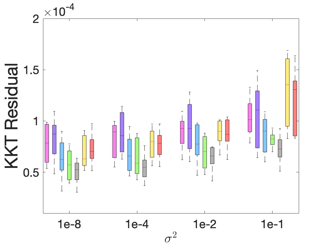
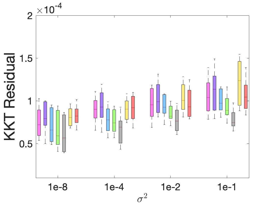
Figure 1: KKT residual box plots over 47 CUTEst problems with given initialization (left) and random initialization (right). Each panel has four different noise levels. For each noise level, the first four boxes correspond to TR-SQP-STORM with different types of ${\bar{H}}_{k}$; the fifth box corresponds to TR-SQP-STORM2; and the last two boxes correspond to $\ell_{2}$-SSQP and AL-SSQP, respectively.

The results of the experiment are illustrated in Figure 1. From the figure, we observe that TR-SQP-STORM2 (i.e., our method with second-order stationarity) outperforms the other methods and its superior performance is robust across different noise levels and types of initializations. This advantage is attributed to precise Hessian estimations, the ability to move along negative curvatures, and the computation of SOC steps. Only this method can guarantee to escape from saddle points. Furthermore, at low noise levels ($\sigma^{2}=10^{-8}$ or $10^{-4}$), line-search-based AL-SSQP and $\ell_{2}$-SSQP methods perform comparably to our trust-region methods. However, as noise levels increase, the performance of $\ell_{2}$-SSQP deteriorates rapidly, while AL-SSQP remains competitive though still inferior to our methods. In addition, among the four types of Hessians ${\bar{H}}_{k}$ used in TR-SQP-STORM, we observe that the SR1 update can lead to unstable performance. It achieves small KKT residuals at low noise levels but performs well in some problems and poorly in others at high noise levels. In contrast, the Hessians of EstH and AveH consistently enhance the performance of TR-SQP-STORM across varying noise levels. Notably, AveH demonstrates even better performance than EstH at high noise levels, as Hessian averaging generates more accurate Hessian estimates by aggregating samples.

5.3 Logistic regression

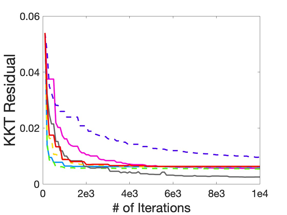
() covtype dataset

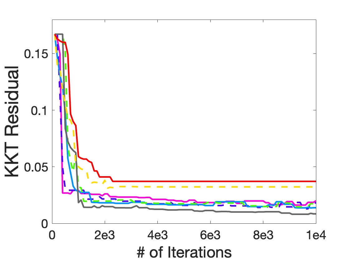
() shuttle dataset

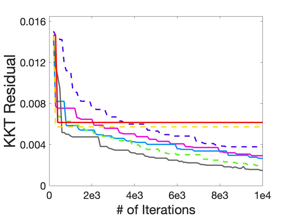
() normal dataset

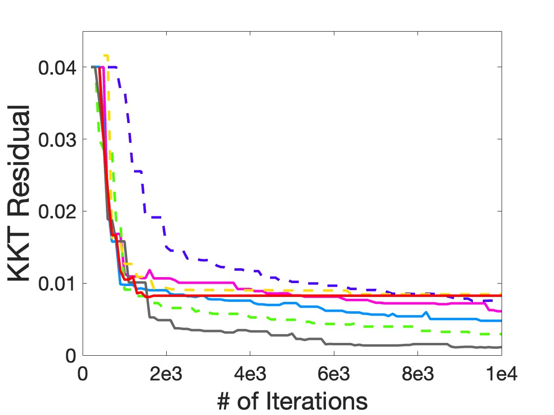
() exponential dataset

Figure 2: Trajectories of KKT residuals of four datasets. Each panel corresponds to a dataset and includes seven lines representing the seven algorithms.

We consider an equality-constrained logistic regression problem of the form:

$$\min_{{\bm{x}}\in\mathbb{R}^{d}}\;\;f({\bm{x}})=\frac{1}{N}\sum_{i=1}^{N}\log\big{(}1+e^{-y_{i}(\bm{z}_{i}^{T}{\bm{x}})}\big{)},\quad\quad\text{s.t.}\quad A{\bm{x}}=\bm{b},$$

where $\{(\bm{z}_{i},y_{i})\}_{i=1}^{N}$ are $N$ samples with features $\bm{z}_{i}\in\mathbb{R}^{d}$ and labels $y_{i}\in\{-1,+1\}$. The constraint parameters $A\in\mathbb{R}^{5\times d}$ and $\bm{b}\in\mathbb{R}^{5}$ are generated for each problem with entries drawn independently from a standard Gaussian distribution while ensuring that $A$ has full row rank. We implement four datasets: covtype and shuttle from the UCI repository, and normal and exponential that are synthetic. For the normal and exponential datasets, we set $d=15$ and $N=6\times 10^{4}$, equally split between the two classes. In the normal dataset, each entry of $\bm{z}_{i}$ is generated from ${\mathcal{N}}(0,1)$ if $y_{i}=1$ and ${\mathcal{N}}(5,1)$ if $y_{i}=-1$. In the exponential dataset, each entry of $\bm{z}_{i}$ is generated from $\exp(1)$ if $y_{i}=1$ and $5+\exp(1)$ if $y_{i}=-1$. We set the initialization to a zero vector. For each algorithm and each dataset, we plot the trajectory of the average KKT residuals over five independent runs. The stopping criteria for TR-SQP-STORM, AL-SSQP, and $\ell_{2}$-SSQP are set as $\|\nabla\mathcal{L}_{k}\|\leq 10^{-4}\text{ OR }k\geq 10^{4}$, while similarly, the stopping criterion for TR-SQP-STORM2 is set as $\max\{\|\nabla\mathcal{L}_{k}\|,\tau_{k}^{+}\}\leq 10^{-4}\text{ OR }k\geq 10^{4}$.

We present the results in Figure 2. From the figure, we observe that TR-SQP-STORM2 clearly outperforms the other methods in three out of four datasets. Only in the shuttle dataset is its performance comparable to TR-SQP-STORM. We also note that AL-SSQP and $\ell_{2}$-SSQP perform well on covtype but poorly on shuttle and normal. For the exponential dataset, the performance of AL-SSQP and $\ell_{2}$-SSQP is similar to that of TR-SQP-STORM with the Id and SR1 Hessian updates, both of which are inferior to the performance with EstH and AveH updates. Overall, among the four types of Hessian matrices tested for TR-SQP-STORM, the averaged Hessian generally performs the best, followed by the estimated Hessian, while the SR1 update performs the worst. However, it is worth noting that for the shuttle dataset, all four types of Hessians exhibit similar performance.

5.4 Saddle-point problem

To demonstrate the efficacy of TR-SQP-STORM2 in escaping saddle points compared to TR-SQP-STORM, AL-SSQP and $\ell_{2}$-SSQP methods, we consider the following saddle-point problem:

$$\min_{(x_{1},x_{2})}f(x_{1},x_{2})=2x_{1}+\frac{1}{2}x_{2}^{2}\quad\quad\text{s.t.}\quad\quad x_{1}^{2}+x_{2}^{2}-1=0.$$ (75)

We can check that Problem (75) has two stationary points: a local minima at $(-1,0)$ and a saddle point at $(1,0)$. In this experiment, we initialize all methods randomly within a neighborhood of radius $0.01$ around the saddle point. Following the CUTEst experiment, we generate estimates of objective values, gradients, and Hessians based on their true deterministic quantities. Specifically, we have $F({\bm{x}}_{k};\xi)\sim{\mathcal{N}}(f_{k},\sigma^{2})$, $\nabla F({\bm{x}}_{k};\xi)\sim{\mathcal{N}}(\nabla f_{k},\sigma^{2}(I+\bm{1}\bm{1}^{T}))$, and $[\nabla^{2}F({\bm{x}}_{k};\xi)]_{i,j}=[\nabla^{2}F({\bm{x}}_{k};\xi)]_{j,i}\sim{\mathcal{N}}([\nabla^{2}f_{k}]_{i,j},\sigma^{2})$. We consider four different noise levels $\sigma^{2}\in\{10^{-8},10^{-4},10^{-2},10^{-1}\}$. For each method on each noise level, we perform 5 independent runs and report the averaged trajectories of the KKT residuals and the smallest eigenvalue of the reduced Lagrangian Hessians. The stopping criteria for all methods are set as $\max\{\|\nabla\mathcal{L}_{k}\|,\tau_{k}^{+}\}\leq 10^{-4}\text{ OR }k\geq 10^{4}$.

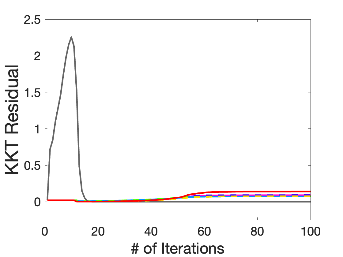
() $\sigma^{2}=10^{-8}$

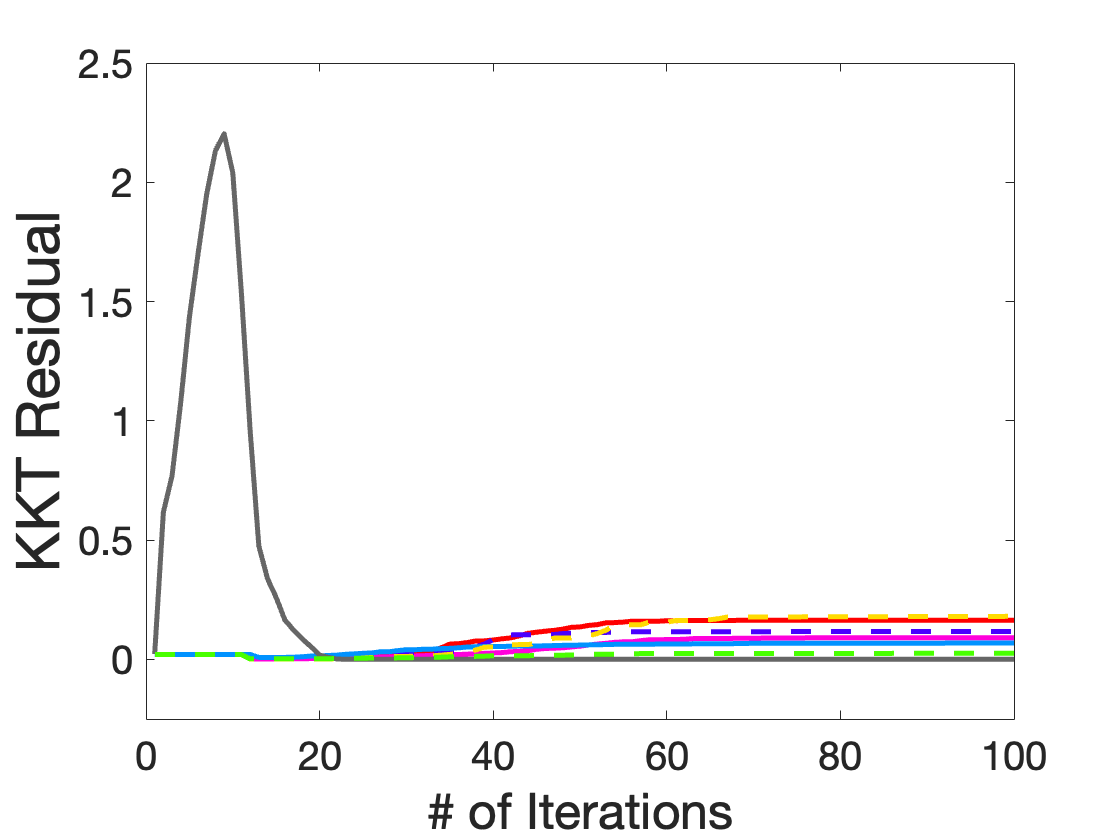
() $\sigma^{2}=10^{-4}$

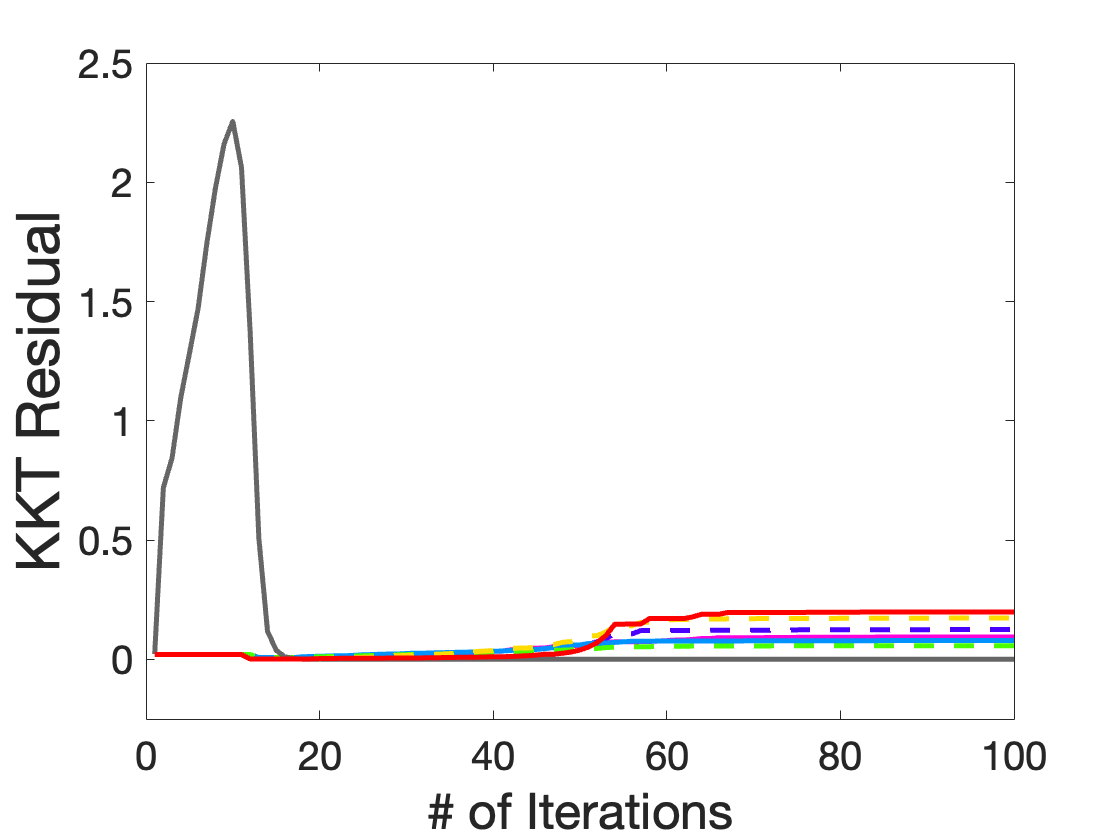
() $\sigma^{2}=10^{-2}$

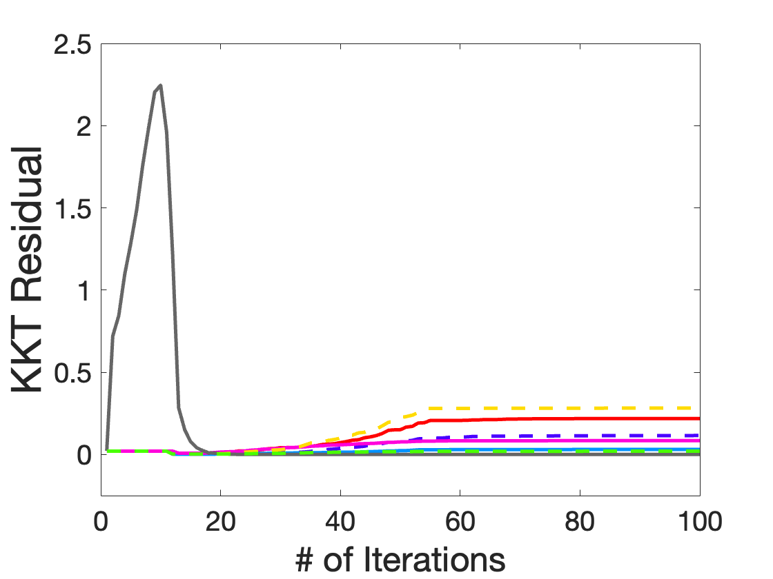
() $\sigma^{2}=10^{-1}$

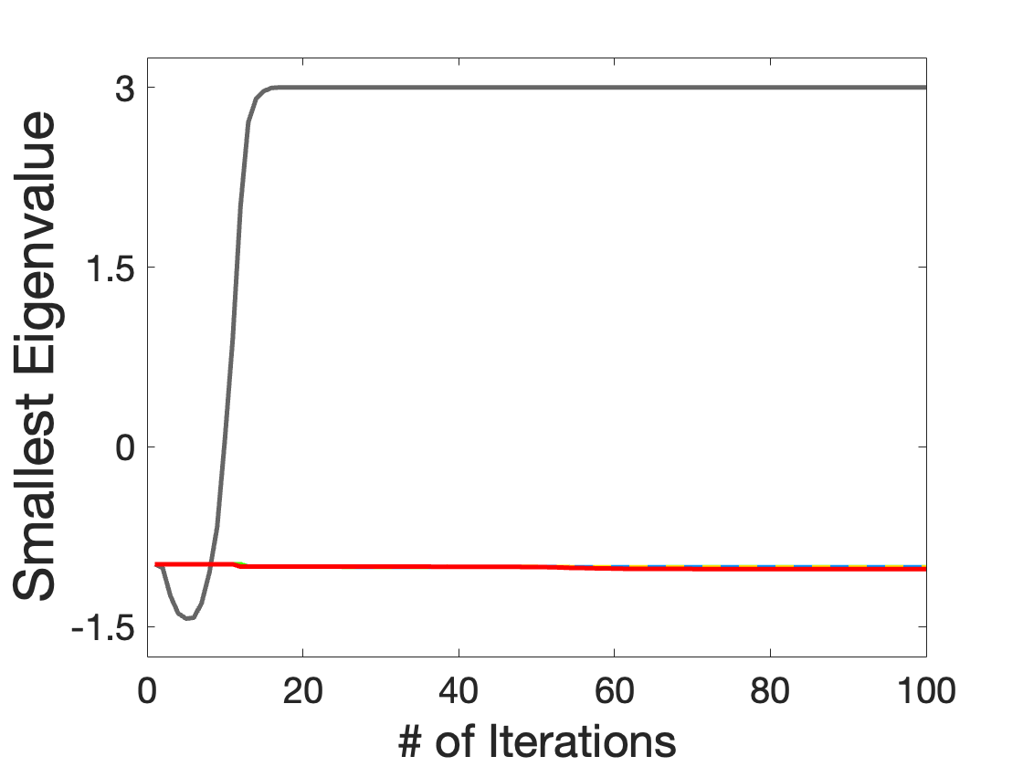
() $\sigma^{2}=10^{-8}$

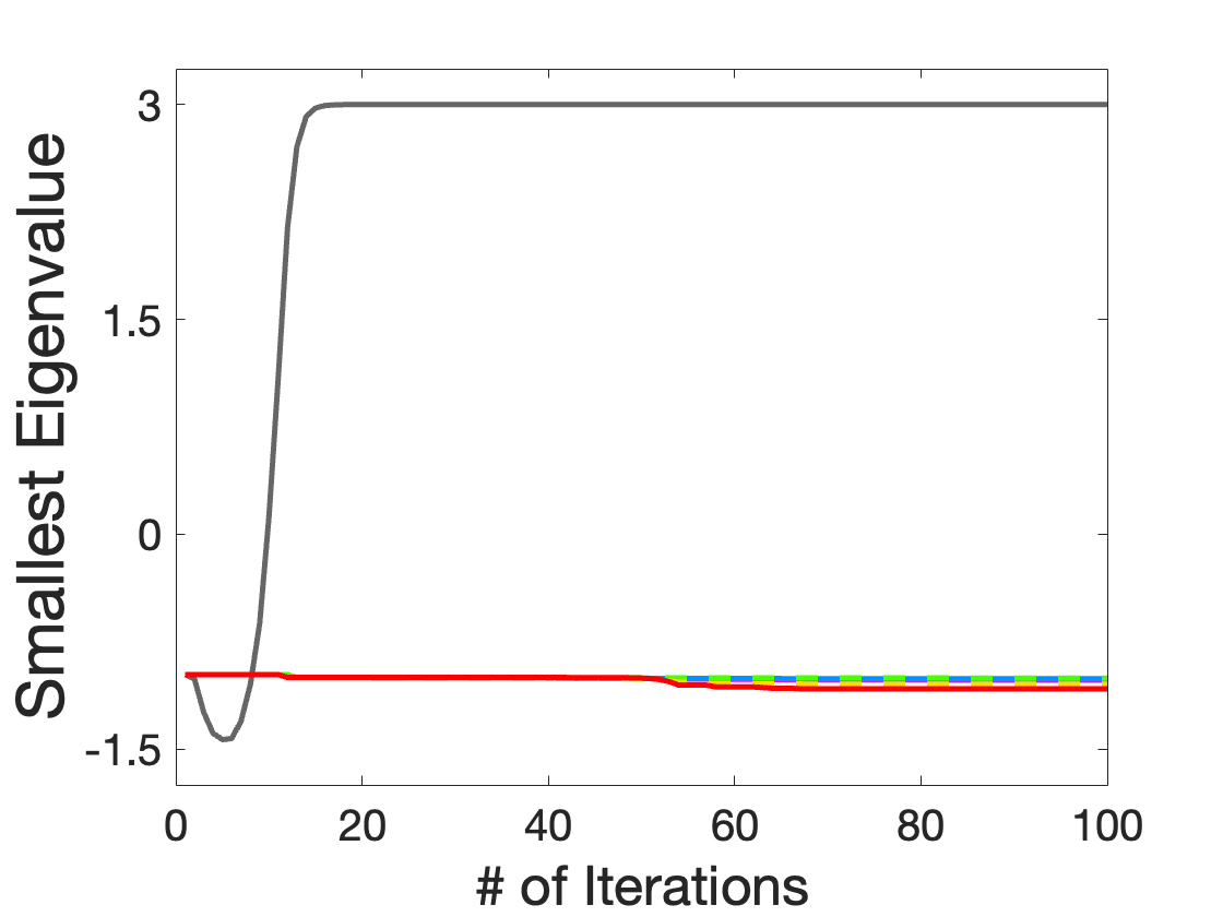
() $\sigma^{2}=10^{-4}$

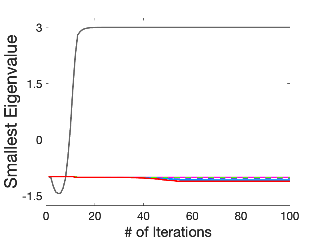
() $\sigma^{2}=10^{-2}$

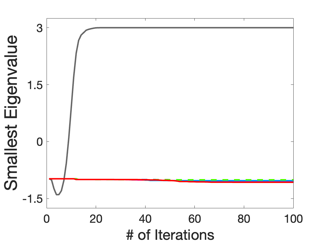
() $\sigma^{2}=10^{-1}$

Figure 3: Trajectories of the KKT residuals and the smallest eigenvalue of the reduced Lagrangian Hessians under four noise levels. The top four figures show the trajectories of the KKT residuals, while the bottom four figures show the trajectories of the smallest eigenvalues. Each figure corresponds to a noise level and includes seven lines representing the seven algorithms.

We present the trajectories of the KKT residuals in Figure 3(a)-(d) and the trajectories of the smallest eigenvalues in Figure 3(e)-(h). To better visualize the results, we plot only the first 100 iterations as both the KKT residuals and the smallest eigenvalues stabilize after this point. From the two figures, we see that across all four noise levels, only TR-SQP-STORM2 successfully escapes the saddle point and converges to the local minima. In contrast, for all other methods, the KKT residuals remain relatively large and the smallest eigenvalues stay close to $-1$, which is precisely the negative curvature at the saddle point $(1,0)$. Thus, we conclude that the other methods are trapped near the saddle point. Moreover, TR-SQP-STORM2 demonstrates a rapid escape, consistently terminating after around 20 iterations for different noise levels.

6 Conclusion

In this paper, we proposed a Trust-Region Sequential Quadratic Programming method called TR-SQP-STORM to find both first- and second-order stationary points for constrained stochastic problems. Our method utilizes a random model framework to represent the objective function. At each iteration, a batch of samples is realized to estimate the objective quantities, with the batch size adaptively selected to ensure the estimators satisfy certain proper accuracy conditions with a fixed probability. We designed two types of trial steps, gradient steps and eigen steps, both of which are computed via a novel parameter-free decomposition of the step and the trust-region radius. The gradient steps aim to reduce the KKT residuals to achieve first-order stationarity, while the eigen steps aim to explore the negative curvature of the reduced Lagrangian Hessian to achieve second-order stationarity. For the latter goal, we additionally computed second-order correction steps to overcome the potential Maratos effect, which occurs exculsively in constrained problems. Under mild assumptions, we showed global almost sure convergence guarantees. Numerical experiments on CUTEst benchmark problems, constrained logistic regression problems, and saddle-point problems illustrate the promising performance of our method.

Appendix A Proof of Lemma 4.19

It suffices to show that (23) is satisfied as long as ${\bar{\mu}}_{k}$ exceeds a deterministic threshold independent of $k$. We divide our analysis into two cases, depending on whether the gradient step or the eigen step is taken.

$\bullet$ Case 1: gradient step is taken. By the algorithm design, a gradient step is taken if and only if (20) holds. Thus, we only need to show

$$\text{Pred}_{k}\leq-\frac{\kappa_{fcd}}{2}\|\bar{\nabla}{\mathcal{L}}_{k}\|\min\left\{\Delta_{k},\frac{\|\bar{\nabla}{\mathcal{L}}_{k}\|}{\|{\bar{H}}_{k}\|}\right\}$$ (A.1)

when ${\bar{\mu}}_{k}$ is sufficiently large. Since $\|c_{k}+G_{k}\Delta{\bm{x}}_{k}\|-\|c_{k}\|=-{\bar{\gamma}}_{k}\|c_{k}\|$, we have

$$\text{Pred}_{k} \stackrel{{\scriptstyle\mathclap{\eqref{def:Pred_k}}}}{{=}}{\bar{g}}_{k}^{T}\Delta{\bm{x}}_{k}+\frac{1}{2}\Delta{\bm{x}}_{k}^{T}{\bar{H}}_{k}\Delta{\bm{x}}_{k}+{\bar{\mu}}_{k}(\|c_{k}+G_{k}\Delta{\bm{x}}_{k}\|-\|c_{k}\|)$$

$$=({\bar{g}}_{k}+{\bar{\gamma}}_{k}{\bar{H}}_{k}{\bm{v}}_{k})^{T}Z_{k}{\bm{u}}_{k}+\frac{1}{2}{\bm{u}}_{k}^{T}Z_{k}^{T}{\bar{H}}_{k}Z_{k}{\bm{u}}_{k}+{\bar{\gamma}}_{k}{\bar{g}}_{k}^{T}{\bm{v}}_{k}+\frac{1}{2}{\bar{\gamma}}_{k}^{2}{\bm{v}}_{k}^{T}{\bar{H}}_{k}{\bm{v}}_{k}-{\bar{\mu}}_{k}{\bar{\gamma}}_{k}\|c_{k}\|$$

$$\leq-\frac{\kappa_{fcd}}{2}\|Z_{k}^{T}({\bar{g}}_{k}+{\bar{\gamma}}_{k}{\bar{H}}_{k}{\bm{v}}_{k})\|\min\left\{\widetilde{\Delta}_{k},\frac{\|Z_{k}^{T}({\bar{g}}_{k}+{\bar{\gamma}}_{k}{\bar{H}}_{k}{\bm{v}}_{k})\|}{\|{\bar{H}}_{k}\|}\right\}+{\bar{\gamma}}_{k}\|{\bar{g}}_{k}\|\|{\bm{v}}_{k}\|$$

$$\quad+\frac{1}{2}{\bar{\gamma}}_{k}\|{\bar{H}}_{k}\|\|{\bm{v}}_{k}\|^{2}-{\bar{\mu}}_{k}{\bar{\gamma}}_{k}\|c_{k}\|,$$ (A.2)

where the inequality is due to (9) and ${\bar{\gamma}}_{k}\leq 1$. By $\|Z_{k}^{T}({\bar{g}}_{k}+{\bar{\gamma}}_{k}{\bar{H}}_{k}{\bm{v}}_{k})\|\geq\|Z_{k}^{T}{\bar{g}}_{k}\|-{\bar{\gamma}}_{k}\|{\bar{H}}_{k}\|\|{\bm{v}}_{k}\|$, we have

$$\|Z_{k}^{T} ({\bar{g}}_{k}+{\bar{\gamma}}_{k}{\bar{H}}_{k}{\bm{v}}_{k})\|\min\left\{\widetilde{\Delta}_{k},\frac{\|Z_{k}^{T}({\bar{g}}_{k}+{\bar{\gamma}}_{k}{\bar{H}}_{k}{\bm{v}}_{k})\|}{\|{\bar{H}}_{k}\|}\right\}$$

$$\geq\|Z_{k}^{T}{\bar{g}}_{k}\|\min\left\{\widetilde{\Delta}_{k},\frac{\|Z_{k}^{T}{\bar{g}}_{k}\|}{\|{\bar{H}}_{k}\|}-{\bar{\gamma}}_{k}\|{\bm{v}}_{k}\|\right\}-{\bar{\gamma}}_{k}\|{\bar{H}}_{k}\|\|{\bm{v}}_{k}\|\min\left\{\widetilde{\Delta}_{k},\frac{\|Z_{k}^{T}{\bar{g}}_{k}\|}{\|{\bar{H}}_{k}\|}-{\bar{\gamma}}_{k}\|{\bm{v}}_{k}\|\right\}$$

$$\geq\|Z_{k}^{T}{\bar{g}}_{k}\|\min\left\{\widetilde{\Delta}_{k},\frac{\|Z_{k}^{T}{\bar{g}}_{k}\|}{\|{\bar{H}}_{k}\|}\right\}-{\bar{\gamma}}_{k}\|Z_{k}^{T}{\bar{g}}_{k}\|\|{\bm{v}}_{k}\|-{\bar{\gamma}}_{k}\|{\bar{H}}_{k}\|\|{\bm{v}}_{k}\|\widetilde{\Delta}_{k}.$$ (A.3)

Combining (A), (A), the fact $\|{\bm{v}}_{k}\|\leq\frac{1}{\sqrt{\kappa_{1,G}}}\|c_{k}\|$, and Assumption 4.1, we obtain

$$\text{Pred}_{k} \leq-\frac{\kappa_{fcd}}{2}\|Z_{k}^{T}{\bar{g}}_{k}\|\min\left\{\widetilde{\Delta}_{k},\frac{\|Z_{k}^{T}{\bar{g}}_{k}\|}{\|{\bar{H}}_{k}\|}\right\}+\frac{\kappa_{fcd}}{2\sqrt{\kappa_{1,G}}}{\bar{\gamma}}_{k}\|Z_{k}^{T}{\bar{g}}_{k}\|\|c_{k}\|+\frac{\kappa_{fcd}}{2\sqrt{\kappa_{1,G}}}{\bar{\gamma}}_{k}\|{\bar{H}}_{k}\|\|c_{k}\|\widetilde{\Delta}_{k}$$

$$\quad+\frac{1}{\sqrt{\kappa_{1,G}}}{\bar{\gamma}}_{k}\|{\bar{g}}_{k}\|\|c_{k}\|+\frac{\kappa_{c}}{2\kappa_{1,G}}{\bar{\gamma}}_{k}\|{\bar{H}}_{k}\|\|c_{k}\|-{\bar{\mu}}_{k}{\bar{\gamma}}_{k}\|c_{k}\|$$

$$\leq-\frac{\kappa_{fcd}}{2}\|Z_{k}^{T}{\bar{g}}_{k}\|\min\left\{\widetilde{\Delta}_{k},\frac{\|Z_{k}^{T}{\bar{g}}_{k}\|}{\|{\bar{H}}_{k}\|}\right\}+\left(\frac{\Delta_{\max}}{2\sqrt{\kappa_{1,G}}}+\frac{\kappa_{c}}{2\kappa_{1,G}}\right){\bar{\gamma}}_{k}\|{\bar{H}}_{k}\|\|c_{k}\|$$

$$\quad+\frac{1.5}{\sqrt{\kappa_{1,G}}}{\bar{\gamma}}_{k}\|{\bar{g}}_{k}\|\|c_{k}\|-{\bar{\mu}}_{k}{\bar{\gamma}}_{k}\|c_{k}\|,$$

where the second inequality uses $\|Z_{k}^{T}{\bar{g}}_{k}\|\leq\|{\bar{g}}_{k}\|$, $\widetilde{\Delta}_{k}\leq\Delta_{\max}$, and $\kappa_{fcd}\leq 1$. By Assumptions 4.1 and 4.18, we know $\|{\bar{g}}_{k}\|\leq\|{\bar{g}}_{k}-g_{k}\|+\|g_{k}\|\leq M+\kappa_{\nabla f}$. Noting that $\|Z_{k}^{T}{\bar{g}}_{k}\|=\|\bar{\nabla}_{{\bm{x}}}{\mathcal{L}}_{k}\|$ and $\|{\bar{H}}_{k}\|\leq\kappa_{B}$ (cf. Assumption 4.18), we further have

$$\text{Pred}_{k}\leq-\frac{\kappa_{fcd}}{2}\|\bar{\nabla}_{{\bm{x}}}{\mathcal{L}}_{k}\|\min\left\{\widetilde{\Delta}_{k},\frac{\|\bar{\nabla}_{{\bm{x}}}{\mathcal{L}}_{k}\|}{\|{\bar{H}}_{k}\|}\right\}+\left\{\frac{\Delta_{\max}\kappa_{B}}{2\sqrt{\kappa_{1,G}}}+\frac{\kappa_{c}\kappa_{B}}{2\kappa_{1,G}}+\frac{1.5(M+\kappa_{\nabla f})}{\sqrt{\kappa_{1,G}}}-{\bar{\mu}}_{k}\right\}{\bar{\gamma}}_{k}\|c_{k}\|.$$ (A.4)

$\bullet$ Case 1a: $\widetilde{\Delta}_{k}\leq\|\bar{\nabla}_{{\bm{x}}}{\mathcal{L}}_{k}\|/\|{\bar{H}}_{k}\|$. We note that

$$-\frac{\kappa_{fcd}}{2}\|\bar{\nabla}_{{\bm{x}}}{\mathcal{L}}_{k}\|\widetilde{\Delta}_{k}-\frac{\kappa_{fcd}}{2}\|\bar{\nabla}_{{\bm{x}}}{\mathcal{L}}_{k}\|\breve{\Delta}_{k}-\frac{\kappa_{fcd}}{2}\|c_{k}\|\Delta_{k}\leq-\frac{\kappa_{fcd}}{2}\|\bar{\nabla}_{{\bm{x}}}{\mathcal{L}}_{k}\|\Delta_{k}-\frac{\kappa_{fcd}}{2}\|c_{k}\|\Delta_{k}\\ \leq-\frac{\kappa_{fcd}}{2}\|\bar{\nabla}{\mathcal{L}}_{k}\|\Delta_{k}\leq-\frac{\kappa_{fcd}}{2}\|\bar{\nabla}{\mathcal{L}}_{k}\|\min\left\{\Delta_{k},\frac{\|\bar{\nabla}{\mathcal{L}}_{k}\|}{\|{\bar{H}}_{k}\|}\right\}.$$

Therefore, we know from (A.4) and the above display that (A.1) holds as long as

$${\bar{\mu}}_{k}{\bar{\gamma}}_{k}\|c_{k}\|\geq\frac{\kappa_{fcd}}{2}\|\bar{\nabla}_{{\bm{x}}}{\mathcal{L}}_{k}\|\breve{\Delta}_{k}+\frac{\kappa_{fcd}}{2}\|c_{k}\|\Delta_{k}+\left\{\frac{\Delta_{\max}\kappa_{B}}{2\sqrt{\kappa_{1,G}}}+\frac{\kappa_{c}\kappa_{B}}{2\kappa_{1,G}}+\frac{1.5(M+\kappa_{\nabla f})}{\sqrt{\kappa_{1,G}}}\right\}{\bar{\gamma}}_{k}\|c_{k}\|.$$ (A.5)

When ${\bar{\gamma}}_{k}=1$, (A.5) holds as long as

$${\bar{\mu}}_{k}\geq\frac{\kappa_{fcd}\|\bar{\nabla}_{{\bm{x}}}{\mathcal{L}}_{k}\|}{2\|c_{k}\|}\breve{\Delta}_{k}+\frac{\kappa_{fcd}}{2}\Delta_{k}+\frac{\Delta_{\max}\kappa_{B}}{2\sqrt{\kappa_{1,G}}}+\frac{\kappa_{c}\kappa_{B}}{2\kappa_{1,G}}+\frac{1.5(M+\kappa_{\nabla f})}{\sqrt{\kappa_{1,G}}}.$$ (A.6)

Noting that

$$\breve{\Delta}_{k}\stackrel{{\scriptstyle\eqref{eq:breve and tilde_delta_k}}}{{=}}\frac{\|c_{k}^{RS}\|}{\|\bar{\nabla}{\mathcal{L}}_{k}^{RS}\|}\Delta_{k}\stackrel{{\scriptstyle\eqref{nequ:1}}}{{=}}\frac{\|G_{k}\|^{-1}\|c_{k}\|}{\|(\|{\bar{H}}_{k}\|^{-1}\bar{\nabla}_{{\bm{x}}}{\mathcal{L}}_{k},\|G_{k}\|^{-1}c_{k})\|}\Delta_{k}\leq\frac{\|G_{k}\|^{-1}\|c_{k}\|}{\|{\bar{H}}_{k}\|^{-1}\|\bar{\nabla}_{{\bm{x}}}{\mathcal{L}}_{k}\|}\Delta_{k},$$

we see (A.6) is satisfied if

$${\bar{\mu}}_{k}\geq\frac{\kappa_{fcd}}{2}\frac{\|{\bar{H}}_{k}\|}{\|G_{k}\|}\Delta_{k}+\frac{\kappa_{fcd}}{2}\Delta_{k}+\frac{\Delta_{\max}\kappa_{B}}{2\sqrt{\kappa_{1,G}}}+\frac{\kappa_{c}\kappa_{B}}{2\kappa_{1,G}}+\frac{1.5(M+\kappa_{\nabla f})}{\sqrt{\kappa_{1,G}}}.$$

Combining the above display with $\Delta_{k}\leq\Delta_{\max}$, $\|G_{k}\|\geq\sqrt{\kappa_{1,G}}$, $\|{\bar{H}}_{k}\|\leq\kappa_{B}$, and $\kappa_{fcd}\leq 1$, we know (A.1) holds if

$${\bar{\mu}}_{k}\geq\left(\frac{\kappa_{B}}{\sqrt{\kappa_{1,G}}}+0.5\right)\Delta_{\max}+\frac{\kappa_{c}\kappa_{B}}{2\kappa_{1,G}}+\frac{1.5(M+\kappa_{\nabla f})}{\sqrt{\kappa_{1,G}}}\eqqcolon\widehat{\mu}_{1}.$$

On the other hand, when ${\bar{\gamma}}_{k}=\breve{\Delta}_{k}/\|{\bm{v}}_{k}\|$, (A.5) holds provided that

$${\bar{\mu}}_{k} \geq\frac{\kappa_{fcd}}{2}\frac{\|\bar{\nabla}_{{\bm{x}}}{\mathcal{L}}_{k}\|\|{\bm{v}}_{k}\|}{\|c_{k}\|}+\frac{\kappa_{fcd}}{2}\frac{\Delta_{k}\|{\bm{v}}_{k}\|}{\breve{\Delta}_{k}}+\frac{\Delta_{\max}\kappa_{B}}{2\sqrt{\kappa_{1,G}}}+\frac{\kappa_{c}\kappa_{B}}{2\kappa_{1,G}}+\frac{1.5(M+\kappa_{\nabla f})}{\sqrt{\kappa_{1,G}}}$$

$$=\frac{\kappa_{fcd}}{2}\frac{\|\bar{\nabla}_{{\bm{x}}}{\mathcal{L}}_{k}\|\|{\bm{v}}_{k}\|}{\|c_{k}\|}+\frac{\kappa_{fcd}}{2}\frac{\|G_{k}\|\|{\bm{v}}_{k}\|\|\bar{\nabla}{\mathcal{L}}_{k}^{RS}\|}{\|c_{k}\|}+\frac{\Delta_{\max}\kappa_{B}}{2\sqrt{\kappa_{1,G}}}+\frac{\kappa_{c}\kappa_{B}}{2\kappa_{1,G}}+\frac{1.5(M+\kappa_{\nabla f})}{\sqrt{\kappa_{1,G}}}.$$ (A.7)

Since $\kappa_{fcd}\leq 1$, $\|{\bm{v}}_{k}\|\leq\|c_{k}\|/\sqrt{\kappa_{1,G}}$, $\|\bar{\nabla}_{{\bm{x}}}{\mathcal{L}}_{k}\|\leq\|{\bar{g}}_{k}\|\leq M+\kappa_{\nabla f}$, and

$$\|\bar{\nabla}{\mathcal{L}}_{k}^{RS}\|\leq\max\{\|{\bar{H}}_{k}\|^{-1},\|G_{k}\|^{-1}\}\|\bar{\nabla}{\mathcal{L}}_{k}\| \leq\max\left\{\frac{1}{\kappa_{B}},\frac{1}{\sqrt{\kappa_{1,G}}}\right\}(\|\bar{\nabla}_{{\bm{x}}}{\mathcal{L}}_{k}\|+\|c_{k}\|)$$

$$\leq\max\left\{\frac{1}{\kappa_{B}},\frac{1}{\sqrt{\kappa_{1,G}}}\right\}(M+\kappa_{\nabla f}+\kappa_{c}),$$

we know (A) is implied by

$${\bar{\mu}}_{k}\geq\frac{2(M+\kappa_{\nabla f})}{\sqrt{\kappa_{1,G}}}+\frac{\sqrt{\kappa_{2,G}}}{2\sqrt{\kappa_{1,G}}}\max\left\{\frac{1}{\kappa_{B}},\frac{1}{\sqrt{\kappa_{1,G}}}\right\}(M+\kappa_{\nabla f}+\kappa_{c})+\frac{\Delta_{\max}\kappa_{B}}{2\sqrt{\kappa_{1,G}}}+\frac{\kappa_{c}\kappa_{B}}{2\kappa_{1,G}}\eqqcolon\widehat{\mu}_{2}.$$

$\bullet$ Case 1b: $\widetilde{\Delta}_{k}>\|\bar{\nabla}_{{\bm{x}}}{\mathcal{L}}_{k}\|/\|{\bar{H}}_{k}\|$. We note that

$$-\frac{\kappa_{fcd}}{2}\frac{\|\bar{\nabla}_{{\bm{x}}}{\mathcal{L}}_{k}\|^{2}}{\|{\bar{H}}_{k}\|}-\frac{\kappa_{fcd}}{2}\frac{\|c_{k}\|^{2}}{\|{\bar{H}}_{k}\|}=-\frac{\kappa_{fcd}}{2}\frac{\|\bar{\nabla}{\mathcal{L}}_{k}\|^{2}}{\|{\bar{H}}_{k}\|}\leq-\frac{\kappa_{fcd}}{2}\|\bar{\nabla}{\mathcal{L}}_{k}\|\min\left\{\Delta_{k},\frac{\|\bar{\nabla}{\mathcal{L}}_{k}\|}{\|{\bar{H}}_{k}\|}\right\}.$$

Thus, (A.4) suggests that (A.1) holds as long as

$${\bar{\mu}}_{k}{\bar{\gamma}}_{k}\|c_{k}\| \geq\frac{\kappa_{fcd}}{2}\frac{\|c_{k}\|^{2}}{\|{\bar{H}}_{k}\|}+\left\{\frac{\Delta_{\max}\kappa_{B}}{2\sqrt{\kappa_{1,G}}}+\frac{\kappa_{c}\kappa_{B}}{2\kappa_{1,G}}+\frac{1.5(M+\kappa_{\nabla f})}{\sqrt{\kappa_{1,G}}}\right\}{\bar{\gamma}}_{k}\|c_{k}\|$$

$$\Longleftrightarrow{\bar{\mu}}_{k} \geq\frac{\kappa_{fcd}}{2}\frac{\|c_{k}\|}{{\bar{\gamma}}_{k}\|{\bar{H}}_{k}\|}+\frac{\Delta_{\max}\kappa_{B}}{2\sqrt{\kappa_{1,G}}}+\frac{\kappa_{c}\kappa_{B}}{2\kappa_{1,G}}+\frac{1.5(M+\kappa_{\nabla f})}{\sqrt{\kappa_{1,G}}}.$$ (A.8)

By (6), $\widetilde{\Delta}_{k}>\|\bar{\nabla}_{{\bm{x}}}{\mathcal{L}}_{k}\|/\|{\bar{H}}_{k}\|=\|\bar{\nabla}_{{\bm{x}}}{\mathcal{L}}_{k}^{RS}\|$ implies $\Delta_{k}>\|\bar{\nabla}{\mathcal{L}}_{k}^{RS}\|$. Using $\breve{\Delta}_{k}=\|G_{k}\|^{-1}\|c_{k}\|/\|\bar{\nabla}{\mathcal{L}}_{k}^{RS}\|\cdot\Delta_{k}$ and $\|{\bm{v}}_{k}\|\leq\|c_{k}\|/\sqrt{\kappa_{1,G}}$, we have

$${\bar{\gamma}}_{k}=\min\left\{\frac{\breve{\Delta}_{k}}{\|{\bm{v}}_{k}\|},1\right\}=\min\left\{\frac{\|G_{k}\|^{-1}\|c_{k}\|\Delta_{k}}{\|\bar{\nabla}{\mathcal{L}}_{k}^{RS}\|\|{\bm{v}}_{k}\|},1\right\}\\ \geq\min\left\{\frac{\|c_{k}\|}{\|G_{k}\|\|{\bm{v}}_{k}\|},1\right\}\geq\min\left\{\sqrt{\frac{\kappa_{1,G}}{\kappa_{2,G}}},1\right\}=\sqrt{\frac{\kappa_{1,G}}{\kappa_{2,G}}}.$$

Thus, with $\kappa_{fcd}\leq 1$, (A) (and hence (A.1)) is implied by

$${\bar{\mu}}_{k}\geq\frac{\kappa_{c}}{2\kappa_{B}}\sqrt{\frac{\kappa_{2,G}}{\kappa_{1,G}}}+\frac{\Delta_{\max}\kappa_{B}}{2\sqrt{\kappa_{1,G}}}+\frac{\kappa_{c}\kappa_{B}}{2\kappa_{1,G}}+\frac{1.5(M+\kappa_{\nabla f})}{\sqrt{\kappa_{1,G}}}\eqqcolon\widehat{\mu}_{3}.$$ (A.9)

$\bullet$ Case 2: eigen step is taken. We only need to show

$$\text{Pred}_{k}\leq-\frac{\kappa_{fcd}}{2}{\bar{\tau}}_{k}^{+}\Delta_{k}^{2}-\frac{\kappa_{fcd}}{2}{\bar{\tau}}_{k}^{+}\|c_{k}\|\Delta_{k}$$ (A.10)

when ${\bar{\mu}}_{k}$ is sufficiently large. By the definition of the eigen step, we have

$$\text{Pred}_{k} \stackrel{{\scriptstyle\mathclap{\eqref{def:Pred_k}}}}{{=}}{\bar{g}}_{k}^{T}\Delta{\bm{x}}_{k}+\frac{1}{2}\Delta{\bm{x}}_{k}^{T}{\bar{H}}_{k}\Delta{\bm{x}}_{k}+{\bar{\mu}}_{k}(\|c_{k}+G_{k}\Delta{\bm{x}}_{k}\|-\|c_{k}\|)$$

$$=({\bar{g}}_{k}+{\bar{\gamma}}_{k}{\bar{H}}_{k}{\bm{v}}_{k})^{T}Z_{k}{\bm{u}}_{k}+\frac{1}{2}{\bm{u}}_{k}^{T}Z_{k}^{T}{\bar{H}}_{k}Z_{k}{\bm{u}}_{k}+{\bar{\gamma}}_{k}{\bar{g}}_{k}^{T}{\bm{v}}_{k}+\frac{1}{2}{\bar{\gamma}}_{k}^{2}{\bm{v}}_{k}^{T}{\bar{H}}_{k}{\bm{v}}_{k}-{\bar{\mu}}_{k}{\bar{\gamma}}_{k}\|c_{k}\|$$

$$\stackrel{{\scriptstyle\mathclap{\eqref{eq:reduction_eigen_step}}}}{{\leq}}-\frac{\kappa_{fcd}}{2}{\bar{\tau}}_{k}^{+}\widetilde{\Delta}_{k}^{2}+{\bar{\gamma}}_{k}\|{\bar{g}}_{k}\|\|{\bm{v}}_{k}\|+\frac{1}{2}{\bar{\gamma}}_{k}\|{\bar{H}}_{k}\|\|{\bm{v}}_{k}\|^{2}-{\bar{\mu}}_{k}{\bar{\gamma}}_{k}\|c_{k}\|.$$

By Assumptions 4.1, 4.18 and $\|{\bm{v}}_{k}\|\leq\|c_{k}\|/\sqrt{\kappa_{1,G}}$, we further have

$$\text{Pred}_{k} \leq-\frac{\kappa_{fcd}}{2}{\bar{\tau}}_{k}^{+}\widetilde{\Delta}_{k}^{2}+\frac{M+\kappa_{\nabla f}}{\sqrt{\kappa_{1,G}}}{\bar{\gamma}}_{k}\|c_{k}\|+\frac{\kappa_{c}\kappa_{B}}{2\kappa_{1,G}}{\bar{\gamma}}_{k}\|c_{k}\|-{\bar{\mu}}_{k}{\bar{\gamma}}_{k}\|c_{k}\|$$

$$=-\frac{\kappa_{fcd}}{2}{\bar{\tau}}_{k}^{+}\Delta_{k}^{2}-\frac{\kappa_{fcd}}{2}{\bar{\tau}}_{k}^{+}\|c_{k}\|\Delta_{k}+\frac{\kappa_{fcd}}{2}{\bar{\tau}}_{k}^{+}\breve{\Delta}_{k}^{2}+\frac{\kappa_{fcd}}{2}{\bar{\tau}}_{k}^{+}\|c_{k}\|\Delta_{k}$$

$$\quad+\left\{\frac{M+\kappa_{\nabla f}}{\sqrt{\kappa_{1,G}}}+\frac{\kappa_{c}\kappa_{B}}{2\kappa_{1,G}}-{\bar{\mu}}_{k}\right\}{\bar{\gamma}}_{k}\|c_{k}\|.$$

Thus, (A.10) holds if

$${\bar{\mu}}_{k}{\bar{\gamma}}_{k} \|c_{k}\|\geq\frac{\kappa_{fcd}}{2}{\bar{\tau}}_{k}^{+}\breve{\Delta}_{k}^{2}+\frac{\kappa_{fcd}}{2}{\bar{\tau}}_{k}^{+}\|c_{k}\|\Delta_{k}+\left\{\frac{M+\kappa_{\nabla f}}{\sqrt{\kappa_{1,G}}}+\frac{\kappa_{c}\kappa_{B}}{2\kappa_{1,G}}\right\}{\bar{\gamma}}_{k}\|c_{k}\|$$

$$\stackrel{{\scriptstyle\mathclap{\eqref{eq:breve and tilde_delta_k_2}}}}{{=}}\frac{\kappa_{fcd}}{2}\frac{{\bar{\tau}}_{k}^{+}\|c_{k}^{RS}\|^{2}}{({\bar{\tau}}_{k}^{RS+})^{2}+\|c_{k}^{RS}\|^{2}}\Delta_{k}^{2}+\frac{\kappa_{fcd}}{2}{\bar{\tau}}_{k}^{+}\|c_{k}\|\Delta_{k}+\left\{\frac{M+\kappa_{\nabla f}}{\sqrt{\kappa_{1,G}}}+\frac{\kappa_{c}\kappa_{B}}{2\kappa_{1,G}}\right\}{\bar{\gamma}}_{k}\|c_{k}\|.$$ (A.11)

When ${\bar{\gamma}}_{k}=1$, by Young’s inequality, ${\bar{\tau}}_{k}^{+}\leq\|{\bar{H}}_{k}\|\leq\kappa_{B}$, and $\Delta_{k}\leq\Delta_{\max}$, we know (A) is implied by

$${\bar{\mu}}_{k} \geq\frac{\kappa_{fcd}}{4}\frac{{\bar{\tau}}_{k}^{+}\|c_{k}^{RS}\|}{{\bar{\tau}}_{k}^{RS+}\|c_{k}\|}\Delta_{\max}^{2}+\frac{\kappa_{fcd}}{2}\kappa_{B}\Delta_{\max}+\frac{M+\kappa_{\nabla f}}{\sqrt{\kappa_{1,G}}}+\frac{\kappa_{c}\kappa_{B}}{2\kappa_{1,G}}$$

$$\Longleftarrow{\bar{\mu}}_{k} \geq\frac{\kappa_{fcd}}{4}\frac{\kappa_{B}}{\sqrt{\kappa_{1,G}}}\Delta_{\max}^{2}+\frac{\kappa_{fcd}}{2}\kappa_{B}\Delta_{\max}+\frac{M+\kappa_{\nabla f}}{\sqrt{\kappa_{1,G}}}+\frac{\kappa_{c}\kappa_{B}}{2\kappa_{1,G}}$$

$$\Longleftarrow{\bar{\mu}}_{k} \geq\frac{\kappa_{B}}{4\sqrt{\kappa_{1,G}}}\Delta_{\max}^{2}+\frac{\kappa_{B}\Delta_{\max}}{2}+\frac{M+\kappa_{\nabla f}}{\sqrt{\kappa_{1,G}}}+\frac{\kappa_{c}\kappa_{B}}{2\kappa_{1,G}}\eqqcolon\widehat{\mu}_{4}.$$

When ${\bar{\gamma}}_{k}<1$, without loss of generality, we suppose $\|c_{k}\|\neq 0$ (otherwise (A) is trivial). From (10) and ${\bar{\gamma}}_{k}\|{\bm{v}}_{k}\|=\breve{\Delta}_{k}$, we have

$$\Delta_{k}=\frac{{\bar{\gamma}}_{k}\|{\bm{v}}_{k}\|\|G_{k}\|}{\|c_{k}\|}\|({\bar{\tau}}_{k}^{RS+},c_{k}^{RS})\|.$$

Thus, (A) is equivalent to

$${\bar{\mu}}_{k}{\bar{\gamma}}_{k}\|c_{k}\|\geq\frac{\kappa_{fcd}}{2}{\bar{\tau}}_{k}^{+}{\bar{\gamma}}_{k}^{2}\|{\bm{v}}_{k}\|^{2}+\frac{\kappa_{fcd}}{2}{\bar{\tau}}_{k}^{+}{\bar{\gamma}}_{k}\|{\bm{v}}_{k}\|\|G_{k}\|\|({\bar{\tau}}_{k}^{RS+},c_{k}^{RS})\|+\left\{\frac{M+\kappa_{\nabla f}}{\sqrt{\kappa_{1,G}}}+\frac{\kappa_{c}\kappa_{B}}{2\kappa_{1,G}}\right\}{\bar{\gamma}}_{k}\|c_{k}\|.$$

Since $\max\{{\bar{\gamma}}_{k},\kappa_{fcd}\}\leq 1$, we only need ${\bar{\mu}}_{k}$ to satisfy

$${\bar{\mu}}_{k}\geq\frac{{\bar{\tau}}_{k}^{+}\|{\bm{v}}_{k}\|^{2}}{2\|c_{k}\|}+\frac{{\bar{\tau}}_{k}^{+}\|{\bm{v}}_{k}\|}{2\|c_{k}\|}\|G_{k}\|\|({\bar{\tau}}_{k}^{RS+},c_{k}^{RS})\|+\frac{M+\kappa_{\nabla f}}{\sqrt{\kappa_{1,G}}}+\frac{\kappa_{c}\kappa_{B}}{2\kappa_{1,G}}.$$

Using ${\bar{\tau}}_{k}^{+}\leq\|{\bar{H}}_{k}\|\leq\kappa_{B}$ and $\|{\bm{v}}_{k}\|\leq\|c_{k}\|/\sqrt{\kappa_{1,G}}$, and applying Assumptions 4.1 and 4.18, we know the above display can be further implied by

$${\bar{\mu}}_{k}\geq\frac{\kappa_{c}\kappa_{B}}{\kappa_{1,G}}+\frac{\kappa_{B}\sqrt{\kappa_{2,G}}}{2\sqrt{\kappa_{1,G}}}\left(1+\frac{\kappa_{c}}{\sqrt{\kappa_{1,G}}}\right)+\frac{M+\kappa_{\nabla f}}{\sqrt{\kappa_{1,G}}}\eqqcolon\widehat{\mu}_{5}.$$

Combining all the results above by defining $\widetilde{\mu}=\max\{\widehat{\mu}_{1},\ldots,\widehat{\mu}_{5}\}$, we know (23) is satisfied if ${\bar{\mu}}_{k}\geq\widetilde{\mu}$. Since ${\bar{\mu}}_{k}$ is increased by a factor of $\rho$ for each update, this result suggests that ${\bar{\mu}}_{k}\leq\rho\widetilde{\mu}\eqqcolon{\widehat{\mu}}$. This completes the proof.

References

• Achiam et al. (2017) J. Achiam, D. Held, A. Tamar, and P. Abbeel. Constrained policy optimization. In International conference on machine learning, pages 22–31. PMLR, 2017.
• Bandeira et al. (2012) A. S. Bandeira, K. Scheinberg, and L. N. Vicente. Computation of sparse low degree interpolating polynomials and their application to derivative-free optimization. Mathematical Programming, 134(1):223–257, 2012.
• Bandeira et al. (2014) A. S. Bandeira, K. Scheinberg, and L. N. Vicente. Convergence of trust-region methods based on probabilistic models. SIAM Journal on Optimization, 24(3):1238–1264, 2014.
• Beiser et al. (2023) F. Beiser, B. Keith, S. Urbainczyk, and B. Wohlmuth. Adaptive sampling strategies for risk-averse stochastic optimization with constraints. IMA Journal of Numerical Analysis, 43(6):3729–3765, 2023.
• Berahas et al. (2021) A. S. Berahas, F. E. Curtis, D. Robinson, and B. Zhou. Sequential quadratic optimization for nonlinear equality constrained stochastic optimization. SIAM Journal on Optimization, 31(2):1352–1379, 2021.
• Berahas et al. (2022) A. S. Berahas, R. Bollapragada, and B. Zhou. An adaptive sampling sequential quadratic programming method for equality constrained stochastic optimization. arXiv preprint arXiv:2206.00712, 2022.
• Berahas et al. (2023a) A. S. Berahas, F. E. Curtis, M. J. O’Neill, and D. P. Robinson. A stochastic sequential quadratic optimization algorithm for nonlinear-equality-constrained optimization with rank-deficient jacobians. Mathematics of Operations Research, 2023a.
• Berahas et al. (2023b) A. S. Berahas, J. Shi, Z. Yi, and B. Zhou. Accelerating stochastic sequential quadratic programming for equality constrained optimization using predictive variance reduction. Computational Optimization and Applications, 86(1):79–116, 2023b.
• Berahas et al. (2023c) A. S. Berahas, M. Xie, and B. Zhou. A sequential quadratic programming method with high probability complexity bounds for nonlinear equality constrained stochastic optimization. arXiv preprint arXiv:2301.00477, 2023c.
• Berahas et al. (2024) A. S. Berahas, R. Bollapragada, and J. Shi. Modified line search sequential quadratic methods for equality-constrained optimization with unified global and local convergence guarantees. arXiv preprint arXiv:2406.11144, 2024.
• Bertsekas (1982) D. P. Bertsekas. Constrained Optimization and Lagrange Multiplier Methods. Elsevier, 1982.
• Betts (2010) J. T. Betts. Practical Methods for Optimal Control and Estimation Using Nonlinear Programming. Society for Industrial and Applied Mathematics, 2010.
• Blanchet et al. (2019) J. Blanchet, C. Cartis, M. Menickelly, and K. Scheinberg. Convergence rate analysis of a stochastic trust-region method via supermartingales. INFORMS Journal on Optimization, 1(2):92–119, 2019.
• Boggs and Tolle (1995) P. T. Boggs and J. W. Tolle. Sequential quadratic programming. Acta Numerica, 4:1–51, 1995.
• Bollapragada et al. (2023) R. Bollapragada, C. Karamanli, B. Keith, B. Lazarov, S. Petrides, and J. Wang. An adaptive sampling augmented lagrangian method for stochastic optimization with deterministic constraints. Computers & Mathematics with Applications, 149:239–258, 2023.
• Byrd et al. (1987) R. H. Byrd, R. B. Schnabel, and G. A. Shultz. A trust region algorithm for nonlinearly constrained optimization. SIAM Journal on Numerical Analysis, 24(5):1152–1170, 1987.
• Cao et al. (2023) L. Cao, A. S. Berahas, and K. Scheinberg. First- and second-order high probability complexity bounds for trust-region methods with noisy oracles. Mathematical Programming, 207(1–2):55–106, 2023.
• Chen et al. (2017) R. Chen, M. Menickelly, and K. Scheinberg. Stochastic optimization using a trust-region method and random models. Mathematical Programming, 169(2):447–487, 2017.
• Choromanska et al. (2015) A. Choromanska, M. Henaff, M. Mathieu, G. B. Arous, and Y. LeCun. The loss surfaces of multilayer networks. In Artificial intelligence and statistics, pages 192–204. PMLR, 2015.
• Conn et al. (2000) A. R. Conn, N. I. M. Gould, and P. L. Toint. Trust Region Methods. Society for Industrial and Applied Mathematics, 2000.
• Conn et al. (2009a) A. R. Conn, K. Scheinberg, and L. N. Vicente. Introduction to Derivative-Free Optimization. Society for Industrial and Applied Mathematics, 2009a.
• Conn et al. (2009b) A. R. Conn, K. Scheinberg, and L. N. Vicente. Global convergence of general derivative-free trust-region algorithms to first- and second-order critical points. SIAM Journal on Optimization, 20(1):387–415, 2009b.
• Cuomo et al. (2022) S. Cuomo, V. S. Di Cola, F. Giampaolo, G. Rozza, M. Raissi, and F. Piccialli. Scientific machine learning through physics–informed neural networks: Where we are and what’s next. Journal of Scientific Computing, 92(3), 2022.
• Curtis et al. (2023a) F. E. Curtis, X. Jiang, and Q. Wang. Almost-sure convergence of iterates and multipliers in stochastic sequential quadratic optimization. arXiv preprint arXiv:2308.03687, 2023a.
• Curtis et al. (2023b) F. E. Curtis, V. Kungurtsev, D. P. Robinson, and Q. Wang. A stochastic-gradient-based interior-point algorithm for solving smooth bound-constrained optimization problems. arXiv preprint arXiv:2304.14907, 2023b.
• Curtis et al. (2023c) F. E. Curtis, M. J. O’Neill, and D. P. Robinson. Worst-case complexity of an sqp method for nonlinear equality constrained stochastic optimization. Mathematical Programming, 205(1–2):431–483, 2023c.
• Curtis et al. (2023d) F. E. Curtis, D. P. Robinson, and B. Zhou. Sequential quadratic optimization for stochastic optimization with deterministic nonlinear inequality and equality constraints. arXiv preprint arXiv:2302.14790, 2023d.
• Curtis et al. (2024) F. E. Curtis, D. P. Robinson, and B. Zhou. A stochastic inexact sequential quadratic optimization algorithm for nonlinear equality-constrained optimization. INFORMS Journal on Optimization, 2024.
• Dauphin et al. (2014) Y. N. Dauphin, R. Pascanu, C. Gulcehre, K. Cho, S. Ganguli, and Y. Bengio. Identifying and attacking the saddle point problem in high-dimensional non-convex optimization. Advances in neural information processing systems, 27, 2014.
• El-Alem (1991) M. El-Alem. A global convergence theory for the celis–dennis–tapia trust-region algorithm for constrained optimization. SIAM Journal on Numerical Analysis, 28(1):266–290, 1991.
• Fang et al. (2024) Y. Fang, S. Na, M. W. Mahoney, and M. Kolar. Fully stochastic trust-region sequential quadratic programming for equality-constrained optimization problems. SIAM Journal on Optimization, 34(2):2007–2037, 2024.
• Gould et al. (2014) N. I. M. Gould, D. Orban, and P. L. Toint. Cutest: a constrained and unconstrained testing environment with safe threads for mathematical optimization. Computational Optimization and Applications, 60(3):545–557, 2014.
• Hall and Heyde (2014) P. Hall and C. C. Heyde. Martingale Limit Theory and its Application. Academic press, 2014.
• Heinkenschloss and Ridzal (2014) M. Heinkenschloss and D. Ridzal. A matrix-free trust-region sqp method for equality constrained optimization. SIAM Journal on Optimization, 24(3):1507–1541, 2014.
• Jin et al. (2024) B. Jin, K. Scheinberg, and M. Xie. Sample complexity analysis for adaptive optimization algorithms with stochastic oracles. Mathematical Programming, 2024.
• Khalfan et al. (1993) H. F. Khalfan, R. H. Byrd, and R. B. Schnabel. A theoretical and experimental study of the symmetric rank-one update. SIAM Journal on Optimization, 3(1):1–24, 1993.
• Kuang et al. (2023) W. Kuang, S. Na, and M. Anitescu. Online covariance matrix estimation in stochastic inexact newton methods. In OPT 2023: Optimization for Machine Learning, 2023.
• Lou et al. (2024) Y. Lou, S. Sun, and J. Nocedal. Noise-tolerant optimization methods for the solution of a robust design problem. arXiv preprint arXiv:2401.15007, 2024.
• Lu et al. (2024) Z. Lu, S. Mei, and Y. Xiao. Variance-reduced first-order methods for deterministically constrained stochastic nonconvex optimization with strong convergence guarantees. arXiv preprint arXiv:2409.09906, 2024.
• Na and Mahoney (2022) S. Na and M. W. Mahoney. Statistical inference of constrained stochastic optimization via sketched sequential quadratic programming. arXiv preprint arXiv:2205.13687, 2022.
• Na et al. (2022a) S. Na, M. Anitescu, and M. Kolar. An adaptive stochastic sequential quadratic programming with differentiable exact augmented lagrangians. Mathematical Programming, 199(1–2):721–791, 2022a.
• Na et al. (2022b) S. Na, M. Dereziński, and M. W. Mahoney. Hessian averaging in stochastic newton methods achieves superlinear convergence. Mathematical Programming, 201(1–2):473–520, 2022b.
• Na et al. (2023) S. Na, M. Anitescu, and M. Kolar. Inequality constrained stochastic nonlinear optimization via active-set sequential quadratic programming. Mathematical Programming, 202(1–2):279–353, 2023.
• Nocedal and Wright (2006) J. Nocedal and S. Wright. Numerical Optimization. Springer New York, 2006.
• Omojokun (1989) E. O. Omojokun. Trust region algorithms for optimization with nonlinear equality and inequality constraints. PhD thesis, University of Colorado at Boulder, CO, 1989.
• Oztoprak et al. (2023) F. Oztoprak, R. Byrd, and J. Nocedal. Constrained optimization in the presence of noise. SIAM Journal on Optimization, 33(3):2118–2136, 2023.
• Powell and Yuan (1990) M. J. D. Powell and Y. Yuan. A trust region algorithm for equality constrained optimization. Mathematical Programming, 49(1–3):189–211, 1990.
• Qiu and Kungurtsev (2023) S. Qiu and V. Kungurtsev. A sequential quadratic programming method for optimization with stochastic objective functions, deterministic inequality constraints and robust subproblems. arXiv preprint arXiv:2302.07947, 2023.
• Santoso et al. (2005) T. Santoso, S. Ahmed, M. Goetschalckx, and A. Shapiro. A stochastic programming approach for supply chain network design under uncertainty. European Journal of Operational Research, 167(1):96–115, 2005.
• Sun and Nocedal (2023) S. Sun and J. Nocedal. A trust region method for noisy unconstrained optimization. Mathematical Programming, 202(1–2):445–472, 2023.
• Tropp (2011) J. A. Tropp. User-friendly tail bounds for sums of random matrices. Foundations of Computational Mathematics, 12(4):389–434, 2011.
• Wächter and Biegler (2005) A. Wächter and L. T. Biegler. On the implementation of an interior-point filter line-search algorithm for large-scale nonlinear programming. Mathematical Programming, 106(1):25–57, 2005.
• Çakmak and Özekici (2005) U. Çakmak and S. Özekici. Portfolio optimization in stochastic markets. Mathematical Methods of Operations Research, 63(1):151–168, 2005.