Open-/Closed-loop Active Learning for Data-driven Predictive Control

Abstract

An important question in data-driven control is how to obtain an informative dataset. In this work, we consider the problem of effective data acquisition of an unknown linear system with bounded disturbance for both open-loop and closed-loop stages. The learning objective is to minimize the volume of the set of admissible systems. First, a performance measure based on historical data and the input sequence is introduced to characterize the upper bound of the volume of the set of admissible systems. On the basis of this performance measure, an open-loop active learning strategy is proposed to minimize the volume by actively designing inputs during the open-loop stage. For the closed-loop stage, an closed-loop active learning strategy is designed to select and learn from informative closed-loop data. The efficiency of the proposed closed-loop active learning strategy is proved by showing that the unselected data cannot benefit the learning performance. Furthermore, an adaptive predictive controller is designed in accordance with the proposed data acquisition approach. The recursive feasibility and the stability of the controller are proved by analyzing the effect of the closed-loop active learning strategy. Finally, numerical examples and comparisons illustrate the effectiveness of the proposed data acquisition strategy.

Event-triggered learning, Data-driven predictive control, Active learning.

1 Introduction

Due to the advancements in sensing technology and cyber-physical systems, there has been a growing interest in designing controllers directly from data [1, 2, 3]. As a process of learning from data, a major focus in data-driven control has been on how to enhance learning efficiency. This becomes imperative when resources are limited, or when the control mission needs to be accomplished with in a limited time window. For example, in deep-sea exploration [4] and space exploration [5], data transmission becomes energy-intensive due to factors such as Doppler dispersion and cosmic radiation interference, while the lifespan of these systems is critically restricted by the harsh environmental conditions. The central challenge in this context is the development of an effective solution that actively generates and selects informative data samples. Such a solution would enable a controller with reduced data transmissions and learning time.

When data is randomly generated and collected, learning is often slow and inefficient due to the presence of redundant information [6]. To address this issue, active learning provides a promising solution, thanks to its ability to generate and select data from which it learns [7]. From a systems and control perspective, active learning can be divided into open-loop active learning and closed-loop active learning, corresponding to open-loop and closed-loop control systems, respectively. For both cases, the aim is to maximize a certain data informativity metric. Open-loop active learning actively designs inputs to drive the system to the desirable state for data collection. In contrast, closed-loop active learning maximizes the metric by actively selecting closed-loop data, since the system is driven by the closed-loop controller. Generally, active learning can be classified by the employed metrics. For open-loop active learning, metrics are designed to quantify uncertainty [8, 9], diversity [10], or various information measures [11, 12, 13, 14, 15, 16], e.g., Fisher information matrix and Hankel matrix. We refer readers to [17, 18] for additional designs of metrics and their applications in active learning. Open-loop active learning strategies need to actively drive the system to collect desirable data samples. However, this becomes impossible when a closed-loop system is considered, as the system is fully driven by a closed-loop controller.

For data acquisition in a closed-loop scenario, an important issue is how to make use of closed-loop data. A natural idea is to simply collect every data sample. However, a main drawback of this approach is that the learning algorithm need to be performed with the updated dataset. In response to this conundrum, closed-loop active learning schemes received considerable attention in recent years for their ability to actively select informative closed-loop data based on a certain criterion [19, 20]. Some of the early research contributes to state estimation, where only informative data samples are collected to recover the true state of the system [21, 22]. Inspired by this idea, there has been an increasing interest in recovering unknown system dynamics by actively selecting closed-loop data. Several studies utilized the performance of the learning result as the learning criterion [23, 24, 25, 26, 27, 28, 29, 30, 31, 32]. For instance, Umlauft and Hirche considered Gaussian processes and utilized the uncertainty of the learned model as the criterion [23]. Solowjow et al. considered linear systems and set the mismatch of communication rates between the learned model and the true model as the criterion [25]. In addition to the learning results, some other works focused on the properties of the closed-loop data points [33, 34, 35, 36]. As an example, Zheng et al. employed the distance between the new data sample and the dataset as the learning criterion for lazily adapted constant kinky inference problems [33]. For FIR models, Diao et al. used the magnitude of data variation as the criterion [34]. However, analyzing the informativity of closed-loop data samples of linear systems without prior knowledge of the true system remains an open challenge.

Another topic related to our work is adaptive predictive control, which is widely used due to its ability to handle parameter uncertainties and time-variant parameters [37]. These advantages allow us to address common issues in the considered data-driven control framework, such as the update of the dataset and the learning uncertainty introduced by noisy dataset. The research on model-based adaptive predictive control can be traced back to [38], where nonlinear systems with input constraints were analyzed. Later, several works discussed the convergence of parameter estimates by introducing data-selection methods [39] or additional constraints [40]. Another line of research integrated set-membership identification with robust predictive control where various representations of uncertainties were constructed [41, 42, 43, 44]. To enable data-driven formulations for predictive control, the fundamental lemma approaches and the set-valued approaches are widely utilized. The fundamental lemma, which was proposed by Willems et al. in [45], illustrates that all trajectories of a linear time-invariant system can be captured by a finite collection of trajectories.With this instrumental lemma, various data-driven formulations were proposed for different control configurations [46, 47, 48]. Local linear approximation of nonlinear systems [49] and adaptation for time-varying systems [50] were also considered using this lemma. On the other hand, the set-valued approaches utilize a data-driven formulation of admissible systems consistent with the collected data samples. Some studies analyzed the reachable system states under a given input sequence based on the set of admissible systems and designed robust predictive controllers using these reachable states to replace the prediction of system trajectories given by the true model [51, 52]. However, enabling a stabilizing controller with a reduced number of data samples by actively selecting informative data samples remains unclear for data-driven predictive control. This gap also motivates our investigations in this work. Note that our work is also different from existing results on data-driven predictive control with event-/self-triggered and denial communications [46, 47, 48], where the focuses were on exploring event-triggered/denial data transmission and controller update mechanisms to mitigate communication constraints and ensure stability and performance of the closed-loop system. By contrast, our work considers the scenario where the data generation and transmission processes are not restricted, and our aim is to design learning methods to actively generate and select informative data samples for enhanced data efficiency and accelerated learning by evaluating the informativity of the data samples.

In this work, we consider the scenario that the learning framework consists of two stages: an open-loop stage and a closed-loop stage. During the open-loop stage, the data acquisition is driven by an active learning strategy to generate informative data samples. In the closed-loop stage, a data-driven adaptive predictive controller with an active learning strategy is proposed. The employed closed-loop active learning strategy can detect and learn from informative closed-loop data samples, thereby enhancing control performance. A few challenges, however, need to be addressed to enable our design. First, the informativeness measure of datasets depends on the unknown system dynamics, which makes it difficult to suitably design the input signals during the open-loop stage. Second, the determination of the informativeness of a single data sample could be computationally expensive. The informativeness of a single data sample is related not only to the learning result based on the previous dataset but also to the learning result based on the updated dataset that includes the incoming data sample. Therefore, a computationally efficient metric to evaluate the informativeness of a data sample need to be proposed. Furthermore, the effect of learning-based adaptation also adds to the difficulty of analyzing the closed-loop stability and the recursive feasibility of the predictive controller. The main contributions of this work are summarized as follows:

1. A performance measure that quantifies the volume of the set of admissible systems without utilizing the system responses is proposed for datasets of linear systems with bounded disturbances. Then, we show that the proposed method characterizes the exact volume for datasets with a square data matrix (Lemma 3.6) and an upper bound of the volume in general cases (Theorem 3.8). Based on these results, an open-loop active learning strategy that has no requirement on prior knowledge of the true system is designed to minimize the uncertainty introduced by disturbances by actively design system inputs (Theorem 4.19, Corollary 3.10).

2. To determine the informativeness of a single data sample without actually running the learning algorithm, a simple semidefinite program is formulated as a criterion. Then, a closed-loop active learning strategy which actively selects and learns from the closed-loop data is proposed based on this criterion. We show the inclusion of unselected data samples cannot benefit the learning algorithm to obtain a smaller set of admissible systems and prove the feasibility of the learning algorithm (Theorem 5.25).

3. In the closed-loop stage, an adaptive tube-based data-driven predictive controller is designed by applying the proposed closed-loop active learning strategy. We first show the contraction of tubes under the learning and adaptation strategy (Lemma 5.23). Furthermore, given a suitable dataset, the recursive feasibility and the stability of the proposed learning-based adaptive predictive controller are proved (Theorem 5.30).

The rest of the paper is organized as follows. Section 2 introduces the problems under consideration and provides preliminaries of this work. In Section 3, the measure and the approximation of the admissible set are presented. In Section 4, the active learning strategy is presented. Then, an adaptive predictive controller with a closed-loop active learning strategy is proposed and guarantees on the recursive feasibility and the stability are established in Section 5. Several numerical examples are presented and discussed in Section 6.

Notation: For a matrix $S$, $S_{[i,j]}$ denotes the element at the $i$th row and $j$th column of $S$, $S_{[i]}$ denotes the $i$th column of it, $S_{[i:j]}$ denotes the matrix $\![S_{[i]}\ S_{[i+1]}\dots\ S_{[j]}]$, $\!S^{\top}\!$ denotes its transpose, $\!\det(S)\!$ denotes its determinant, $\!\text{col}(S)\!$ denotes the number of its columns, and $\text{vec}(S)\!:=\![S_{[1]}^{\top}\ S_{[2]}^{\top}\dots\ S_{[\text{col}(S)]}^{\top}]^{\!\top}\!\!$ denotes its vectorization. We write $\!S\!\succ\!0\!$ ($S\!\succeq\!0$) if $\!S\!$ is symmetric and positive (semi-)definite, and we denote negative (semi-)definiteness similarly. Besides, we let $\mathbb{Z}_{\geq 0}$ denote the set of nonnegative integers and write $\mathbb{Z}_{[i,j]}:=\{i,i+1,\dots,j\}$. Let $\|\cdot\|_{2}$ denote the 2-norm of vectors or matrices. We denote by $I_{n}$ the identity matrix of dimension $n$, and by $0_{n}$ the square matrix of dimension $n$, where all elements are zero. When subscripts are not specified, $I$ and $0$ represent the identity matrix and zero matrix of appropriate dimensions, respectively. For two sets $\mathbb{X}$ and $\mathbb{Y}$, Minkowski set addition is defined as $\mathbb{X}\oplus\mathbb{Y}:=\{x+y\ |\ x\in\mathbb{X},y\in\mathbb{Y}\}$, and Minkowski set subtraction is defined similarly as $\mathbb{X}\ominus\mathbb{Y}:=\{x-y\ |\ x\in\mathbb{X},y\in\mathbb{Y}\}$. We also define $\mathcal{D}_{n}:=\{\text{diag}(d_{1},d_{2},\dots,d_{n})\ |\ d_{i}\geq 0,i\in\mathbb{Z}_{[1,n]}\}$.

2 Preliminaries and Problem Formulation

In this paper, we consider a linear time-invariant system

$$x(k+1)=\mathcal{A}x(k)+\mathcal{B}u(k)+w(k)$$ (1)

where $x(k)\!\in\!\mathbb{R}^{n_{x}}$ is the state, $u(k)\!\in\!\mathbb{R}^{n_{u}}$ is the input, $w(k)\!\in\!\mathbb{R}^{n_{x}}$ is the unknown disturbance, and $\mathcal{A}\!\in\!\mathbb{R}^{n_{x}\times n_{x}}$ and $\mathcal{B}\!\in\!\mathbb{R}^{n_{x}\times n_{u}}$ denote the unknown state and input matrices. We assume that $w(k)\in\mathcal{W}$ hold for all $k\in\mathbb{Z}_{\geq 0}$, where $\mathcal{W}:=\left\{w\in\mathbb{R}^{n_{x}}\ |\ w^{\top}w<\delta\right\}$, $\delta>0$. Suppose that the initial state is $x(0)$ and the input sequence applied to the system is $u(i),i\in\mathbb{Z}_{[0,t_{0}-1]}$ where $t_{0}$ represents the experiment time. Then, we denote the states and disturbances of the system corresponding to the input sequence by $x(i),i\in\mathbb{Z}_{[0,t_{0}]}$ and $w(i),i\in\mathbb{Z}_{[0,t_{0}-1]}$, respectively. For compactness, we define $\Delta_{r}:=[\mathcal{A}\ \mathcal{B}]$, $h(i):=[x(i)^{\top}u(i)^{\top}]^{\top}$, $i\in\mathbb{Z}_{[0,t_{0}-1]}$, and $n_{h}:=n_{x}+n_{u}$.

2.1 Matrix Ellipsoids and the Matrix S-Lemma

Before formulating the problem of active learning for adaptive data-driven predictive control, preliminaries about matrix ellipsoids and the matrix S-lemma are introduced first for the legibility and clarity of this work.

Definition 1 (see[53])

For symmetric matrices $E\in\mathbb{R}^{p\times p}$, $G\in\mathbb{R}^{q\times q}$ and matrix $F\in\mathbb{R}^{p\times q}$, we term matrix ellipsoid a set in the following form:

$$\begin{split}\mathcal{E}_{mat}\!:=\!\left\{{Z\!\in\mathbb{R}^{p\times q}\hskip 2.0pt|\hskip 2.0ptZ^{\top}EZ+Z^{\top}F+F^{\top}Z+G\preceq 0}\right\}\end{split}$$ (2)

where $E\!\succ\!0$, ${F^{\top}E^{-1}F-G\!\succ\!0}$. If we let ${Z_{c}\!:=\!-E^{-1}F}$, $G_{c}\!:=\!F^{\top}E^{-1}F-G$, the set in (2) can be reformulated as:

$$\mathcal{E}^{{}^{\prime}}_{mat}:=\left\{{Z\in\mathbb{R}^{p\times q}\hskip 2.0pt|\hskip 2.0pt(Z-Z_{c})^{\top}E(Z-Z_{c})\preceq G_{c}}\right\},$$ (3)

which is another form of matrix ellipsoid. We term ${Z_{c}}$ as the center of $\mathcal{E}_{mat}$. Besides, we also note that ${Z_{c}}$ always belongs to $\mathcal{E}_{mat}$ on the basis of (3).

As an extension to the classical ellipsoids in the Euclidean space [54], the constraint $E\succ 0$ ensures that $\mathcal{E}_{mat}$ is bounded, and the constraint $F^{\top}E^{-1}F-G\succ 0$ ensures that $\mathcal{E}_{mat}$ is not empty or a singleton. Furthermore, the measure of matrix ellipsoids was analyzed using standard measure theory in [53].

Lemma 1 (see [53, Lemma 1])

A matrix ellipsoid is measurable. Consider the matrix ellipsoid $\mathcal{E}_{m}$ defined in (2). A measure $\mu$ can be computed as $\mu(\mathcal{E}_{m})\!:=\!m(\mathcal{V}(\mathcal{E}_{m}))$, where $\!\mathcal{V}(\mathcal{E}_{m})\!:=\!\{\text{vec}(s)\ |\ s\!\in\!\mathcal{E}_{m}\}\!$ and $m(\mathcal{V}(\mathcal{E}_{m}))$ is the Lebesgue measure of the set $\mathcal{V}(\mathcal{E}_{m})$. Accordingly, $\mu(\mathcal{E}_{m})$ can be computed as

$$\mu(\mathcal{E}_{m})=\beta_{m}(\det{(F^{\top}E^{-1}F-G)})^{p/2}(\det{(E^{-1})})^{q/2},$$ (4)

where the constant $\beta_{m}$ depends only on $p$ and $q$, which are the number of rows and columns, respectively, of the matrices that belong to the matrix ellipsoid $\mathcal{E}_{m}$ in (2).

Note that any element in a matrix ellipsoid satisfies a matrix-valued quadratic inequality according to (2). To offer an insight into the matrix quadratic inequalities, the generalized version of the S-lemma was discussed in [55] and is an instrumental ingredient in this work.

Lemma 2 (see [55, Theorem 9])

Let $\tilde{Z}\in\mathbb{R}^{n_{a}\times n_{b}}$, $\tilde{M}$ and $\tilde{N}$ be symmetric matrices in $\mathbb{R}^{(n_{a}+n_{b})\times(n_{a}+n_{b})}$. Assume that there exists some matrix $\bar{Z}\in\mathbb{R}^{n_{a}\times n_{b}}$ such that

$$\begin{bmatrix}I\\ \bar{Z}\end{bmatrix}^{\top}\tilde{N}\begin{bmatrix}I\\ \bar{Z}\end{bmatrix}\succ 0.$$ (5)

Then, the following statements are equivalent:

1. $\begin{bmatrix}I\\ \tilde{Z}\end{bmatrix}^{\top}\tilde{M}\begin{bmatrix}I\\ \tilde{Z}\end{bmatrix}\succeq 0,\forall\tilde{Z}\in\mathbb{R}^{n_{a}\times n_{b}}\hskip 1.99997pt\text{with}\begin{bmatrix}I\\ \tilde{Z}\end{bmatrix}^{\top}\tilde{N}\begin{bmatrix}I\\ \tilde{Z}\end{bmatrix}\succeq 0.$
   

2. There exists a scalar $\alpha\geq 0$ such that $\tilde{M}-\alpha\tilde{N}\succeq 0.$

2.2 Admissible System Ellipsoids

Following the general framework for data-driven analysis and control in [55], we first term a matrix pair $(A,B)$ an admissible system if there exist $w_{s}(k)\!\in\mathcal{W},k\in\mathbb{Z}_{[0,t_{0}-1]}$ such that

$$x(k+1)=Ax(k)+Bu(k)+w_{s}(k),\forall k\in\mathbb{Z}_{[0,t_{0}-1]}.$$ (6)

For compactness, we define

$$\xi(h,\dot{x}):=\begin{bmatrix}I&\dot{x}\\[2.0pt] 0&-h\end{bmatrix}\begin{bmatrix}\delta I&0\\[2.0pt] 0&-I\end{bmatrix}\begin{bmatrix}I&\dot{x}\\[2.0pt] 0&-h\end{bmatrix}^{\top}$$

and $\Delta:=[A\ B]$. Recall that $w_{s}(i)\in\mathcal{W}$. Then, for any admissible system $(A,B)$, we have

$$\begin{bmatrix}I\\[2.0pt] \Delta^{\top}\end{bmatrix}^{\top}\!\xi(h(k),x(k+1))\begin{bmatrix}I\\[2.0pt] \Delta^{\top}\end{bmatrix}\succ 0$$ (7)

holds for all $k\in\mathbb{Z}_{[0,t_{0}-1]}$ based on (6) and the definition of admissible systems. We denote the number of collected data samples as $n$ and group these samples as

$$\begin{split}H&:=[h({d_{1}}),h({d_{2}}),\dots,h(d_{n})],\\ \dot{X}&:=[x({d_{1}\!+\!1}),x({d_{2}\!+\!1}),\dots,x({d_{n}\!+\!1})],\\ \end{split}$$

where $\{d_{1},d_{2},\dots,d_{n}\}\subseteq\mathbb{Z}_{[0,t_{0}-1]}$ is the indices of these samples. Suppose that the corresponding unknown disturbances are $W:=[w({d_{1}}),w({d_{2}}),\dots,w(d_{n})]$. Then, we have

$$\dot{X}=\Delta_{r}H+W$$ (8)

according to (1).

Furthermore, for any matrix $\text{diag}(\lambda_{1},\lambda_{2},\dots,\lambda_{n})\in\mathbb{D}_{n}$, we denote $\text{diag}(\lambda_{1},\lambda_{2},\dots,\lambda_{n})$ as $\Lambda$ and define

$$\Xi(H,\dot{X},\Lambda)\!:=\!\begin{bmatrix}I&\dot{X}\Lambda^{\frac{1}{2}}\\[2.0pt] 0&-H\Lambda^{\frac{1}{2}}\end{bmatrix}\!\begin{bmatrix}\mathrm{tr}(\Lambda)\delta I&0\\[2.0pt] 0&-I\end{bmatrix}\!\begin{bmatrix}I&\dot{X}\Lambda^{\frac{1}{2}}\\[2.0pt] 0&-H\Lambda^{\frac{1}{2}}\end{bmatrix}^{\!\top}\!.$$

We can also derive $\Xi(H,\dot{X},\Lambda)=\sum_{i=1}^{n}\lambda_{i}\xi(H_{[i]},\dot{X}_{[i]})$. Then, on the basis of (7), it follows directly that

$$\begin{bmatrix}I\\[2.0pt] \Delta^{\top}\end{bmatrix}^{\top}\!\Xi(H,\dot{X},\Lambda)\begin{bmatrix}I\\[2.0pt] \Delta^{\top}\end{bmatrix}\succeq 0$$ (9)

holds for any admissible system $(A,B)$. Now, we can formulate a set that captures all admissible systems as

$$\mathcal{C}(H,\dot{X},\Lambda):=\left\{(A,B)\text{ $|$ \eqref{eq:admissible_system} is satisfied}\right\}.$$ (10)

In fact, $\mathcal{C}(H,\dot{X},\Lambda)$ is a matrix ellipsoid under certain conditions on the dataset, as asserted in the following lemma.

Lemma 3

The set $\mathcal{C}(H,\dot{X},\Lambda)$ defined in (10) is a matrix ellipsoid if $H\Lambda H^{\top}\succ 0$.

Proof 2.1.

Based on the definition of $\Xi(H,\dot{X},\Lambda)$, inequality (9) is equivalent to

$$\Delta E_{e}\Delta^{\top}+\Delta F_{e}+(\Delta F_{e})^{\top}+{G_{e}}\preceq 0$$ (11)

where

$$E_{e}\!:=\!H\Lambda H^{\top},F_{e}\!:=\!-H\Lambda\dot{X}^{\top},G_{e}\!:=\!\dot{X}\Lambda\dot{X}^{\top}\!-\mathrm{tr}(\Lambda)\delta I.$$ (12)

The inequality in (11) is in the same form with (2). Then $\mathcal{C}(H,\dot{X},\Lambda)$ is a matrix ellipsoid if $E_{e}\succ 0$ and $F_{e}^{\top}E_{e}^{-1}F_{e}-G_{e}\succ 0$. Note that $E_{e}\succ 0$ follows directly from the condition $H\Lambda H^{\top}\succ 0$. Besides, we can obtain

$$\begin{split}&F_{e}^{\top}E_{e}^{-1}F_{e}-G_{e}\\ &=\dot{X}\Lambda H^{\top}E_{e}^{-1}H\Lambda\dot{X}^{\top}+\mathrm{tr}(\Lambda)\delta I-\dot{X}\Lambda\dot{X}^{\top}\\ &=\dot{X}(\Lambda H^{\top}E_{e}^{-1}H\Lambda-\Lambda)\dot{X}^{\top}+\mathrm{tr}(\Lambda)\delta I.\end{split}$$ (13)

By invoking (8), we have

$$\begin{split}&\dot{X}(\Lambda H^{\top}E_{e}^{-1}H\Lambda-\Lambda)\dot{X}^{\top}\\ &=(\Delta_{r}H+W)(\Lambda H^{\top}E_{e}^{-1}H\Lambda-\Lambda)(\Delta_{r}H+W)^{\top}\end{split}$$ (14)

Note that $H(\Lambda H^{\top}E_{e}^{-1}H\Lambda-\Lambda)=0$ can be verified through standard computations. We can therefore conclude that (14) is equal to $W(\Lambda H^{\top}E_{e}^{-1}H\Lambda-\Lambda)W^{\top}$, and (13) is equal to

$$W\Lambda H^{\top}E_{e}^{-1}H\Lambda W^{\top}+\mathrm{tr}(\Lambda)\delta I-W\Lambda W^{\top}.$$

Since $E_{e}\succ 0$, it follows that $W\Lambda H^{\top}E_{e}^{-1}H\Lambda W^{\top}\succeq 0$. Recall that $H\Lambda H^{\top}\succ 0$ and $\Lambda\in\mathcal{D}_{n}$. There exists $j\in\mathbb{Z}_{[1,n]}$ such that $\lambda_{j}>0$. Moreover, it holds that

$$\mathrm{tr}(\Lambda)\delta I-W\Lambda W^{\top}=\sum\nolimits_{i=1}^{n}\lambda_{i}(\delta I-w(d_{i})w(d_{i})^{\!\top}),$$ (15)

which is positive definite since $w(d_{i})\in\mathcal{W}$ and $\lambda_{j}>0$. Thus, we conclude that $F_{e}^{\top}E_{e}^{-1}F_{e}-G_{e}\succ 0$.

Note that Lemma 3 views the data-driven control from a representative approach perspective and implies that the true system parameter $(\mathcal{A},\mathcal{B})$ lies in a bounded set when the data matrix satisfies a specific condition. Therefore, given the initial state and the input sequence, the future state of the system can be characterized as bounded. A similar result can be found in the context of behavioral approaches, namely, the renown fundamental lemma [45]. The fundamental lemma also provides conditions under which the future trajectory can be uniquely characterized by the initial trajectory and the input sequence. From a systems theory perspective, both approaches investigate the problem of identifiability conditions on the data and have been proved to be equivalent when noise-free data is considered [56].

Remark 2.2.

In this study, we focus on systems with disturbances, hence we posit the assumption that $\delta>0$. However, when we consider noise-free systems by setting $\delta=0$ and $\mathcal{W}=0$, we have

$$\begin{bmatrix}I\\[2.0pt] \Delta^{\top}\end{bmatrix}^{\top}\!\Xi(H,\dot{X},\Lambda)\begin{bmatrix}I\\[2.0pt] \Delta^{\top}\end{bmatrix}=0$$ (16)

holds for any admissible system $\Delta$. Therefore, we can conclude $\Delta E_{e}\Delta^{\top}+\Delta F_{e}+(\Delta F_{e})^{\top}+{G_{e}}=0$, which is equivalent to $(\Delta+F_{e}^{\top}E_{e}^{-1})E_{e}(\Delta+F_{e}^{\top}E_{e}^{-1})^{\top}=0$. Recall that $E_{e}\succ 0$. This implies that (16) has only one solution $\Delta=-F_{e}^{\top}E_{e}^{-1}$, which is equivalent to $\Delta_{r}$ given that $\dot{X}=\Delta_{r}H$.

For brevity, we term $\mathcal{C}(H,\dot{X},\Lambda)$ that satisfies $H\Lambda H^{\top}\succ 0$ as an admissible system ellipsoid (ASE) of (1).

2.3 Problem Formulation

Due to the uncertainty introduced by $w(k)$, the real system cannot be obtained accurately from the dataset. As an alternative, it is easy to observe that $(\mathcal{A},\mathcal{B})\in\mathcal{C}(H,\dot{X},\Lambda)$. Therefore, the data-driven analysis of the true system turns to the set-valued analysis of $\mathcal{C}(H,\dot{X},\Lambda)$ and a smaller ASE implies less uncertainty about the true system. Considering the tradeoff between performance and robustness, it is easier to find a feasible controller to handle the shrunken uncertainty with potentially improved performance guarantee. Since the baseline requirement is to effectively learn a controller to stabilize all systems consistent with the data, we aim to design learning strategies that minimize the volume of the ASE through actively generating and selecting data samples. When the controller is not implemented, we can utilize open-loop active learning strategies with the metric defined as the volume of the ASE. However, the response matrix of the ASE, $\dot{X}$, cannot be directly designed and is not fully accessible in the initial input design and data collection processes, where we have neither a model nor a data-driven representation of the unknown system. Therefore, the the design of inputs need to be performed using only $H$ and $\Lambda$.

With the learned ASE, we design an adaptive tube-based predictive controller for the true system (1). However, when a controller is implemented, the system inputs are determined by the controller and cannot be arbitrarily designed. Thus, we employ a closed-loop active learning strategy that actively selects informative data samples. To mitigate the uncertainties described by the learned ASE, we consider an adaptive tube-based predictive controller with a closed-loop learning strategy (ATDPC) in this work.

In ATDPC, the stage cost function is defined as $l(x,u):=x^{\!\top}Qx+u^{\!\top}Ru$ where $Q\!\in\!\mathbb{R}^{n_{x}\times n_{x}}$ and $R\!\in\!\mathbb{R}^{n_{u}\times n_{u}}$ are positive definite symmetric matrices. The terminal cost function is defined as $V_{f}(x):=x^{\top}P_{T}x$ where $P_{T}\in\mathbb{R}^{n_{x}\times n_{x}}$ is also positive definite and symmetric. The corresponding terminal constraint set is $\mathcal{X}_{T}:=\left\{x\ |\ x^{\top}P_{T}x\leq L_{T}\right\}$ where $L_{T}>0$.

Suppose that the ATDPC is implemented when $k=t_{0}$. Then, according to the classical framework of tube-based model predictive control, we design a dynamic nominal system for $k\geq t_{0}$ as

$$\bar{x}(k+1)=\bar{A}(k)\bar{x}(k)+\bar{B}(k)\bar{u}(k),$$ (17)

where $\bar{\Delta}(k)\!:=\![\bar{A}(k)\ \bar{B}(k)]$ is the center of $\mathcal{C}^{\star}_{k}$, $\mathcal{C}^{\star}_{k}$ is the ASE to be learned based on the closed-loop data at instant $k$, $\bar{x}(k)\in\mathbb{R}^{n_{x}}$ and $\bar{u}(k)\in\mathbb{R}^{n_{u}}$ are the state and input of the nominal system.

To measure the difference between the nominal and the true systems, we define the error between their states as $e(k):=x(k)-\bar{x}(k)$. For a matrix $K\in\mathbb{R}^{n_{x}\times n_{u}}$, the control input applied to (1) is designed as

$$u(k)=Ke(k)+\bar{u}(k),$$ (18)

where the term $Ke(k)$ is designed to reduce the error between the true system and the nominal system. The other term, $\bar{u}(k)$, is designed to control the nominal system to meet the control specifications, constraints, and uncertainties. The value of $\bar{u}(k)$ is obtained by solving:

$$\begin{split}&\min_{\bar{u}_{\text{seq},k}}V_{s}(\bar{x}_{0|k},\bar{u}_{\text{seq},k})\!=\!\sum\nolimits_{i=0}^{N-1}l(\bar{x}_{i|k},\bar{u}_{i|k})+V_{f}(\bar{x}_{N|k})\\ &\ \text{s.t.}\\ &\left\{\begin{array}[]{lc}\bar{x}_{i+1|k}=\bar{A}(k)\bar{x}_{i|k}+\bar{B}(k)\bar{u}_{i|k},\\[4.0pt] \bar{x}_{i|k}\in\mathcal{X}\ominus E_{i|k},\\[4.0pt] \bar{u}_{i|k}\in\mathcal{U}\ominus KE_{i|k},\\[4.0pt] \bar{x}_{N|k}\in\mathcal{X}_{T}\ominus E_{N|k},\\[4.0pt] \bar{x}_{0|k}=x(k),\ E_{0|k}=e(k),\ i\in\mathbb{Z}_{[0,N-1]},\end{array}\right.\end{split}$$ (19)

where $\bar{x}_{0|k}:=\bar{x}(k),\bar{u}_{\text{seq},k}:=(\bar{u}_{0|k},\bar{u}_{1|k},\dots,\bar{u}_{N-1|k})$, $E_{i|k}$ is defined as the reachable error set, where $k\in\mathbb{Z}_{\geq t_{0}}$ and $i\in\mathbb{Z}_{\geq 0}$ indicate that $E_{i|k}$ is the reachable set of $e(i+k)$ computed at instant $k$, i.e., $e(i+k)\in E_{i|k}$. We pick $\bar{u}(k)$ as the optimal $\bar{u}_{0|k}$. The design of $K$, $\mathcal{C}_{k}^{\star}$, $E_{i|k}$, and $L_{T}$ will be investigated in Section 5.

With the statements above, we formally summarized the problems to be solved as follow.

Problem 2.3.

Find a method to quantify the volume of ASEs without utilizing the response matrix, i.e., find a function $\hat{\mu}(H,\Lambda)$ that could characterize the volume of $\mathcal{C}(H,\dot{X},\Lambda)$.

Problem 2.4.

If $\hat{\mu}(\cdot)$ exists, find a method to actively design $u(i)\!\in\!\mathcal{U}_{o}$, $i\in\mathbb{Z}_{[0,t_{0}-1]}$ and $\lambda_{i}\geq 0$, $i\in\mathbb{Z}_{[1,\text{col}(H)]}$ such that $\hat{\mu}(H,\Lambda)$ is minimized.

Problem 2.5.

Once $\hat{\mu}(H,\Lambda)$ is sufficiently small, design an ATDPC as in (18) and (19) that could stabilize (1) and effectively learn from closed-loop data using an active data selecting strategy.

3 Measure and Overapproximation of ASEs

This section focuses on the first problem in Section 2. While Lemma 1 provides a feasible solution to quantify the volume of ASEs, it requires knowledge of $\dot{X}$. To address this issue, the problem is divided into two parts based on the number of data samples. First, we analyze the volume of ASEs with a square data matrix. An effective method that could characterize the accurate volume of the ASE by $H$ and $\Lambda$ is presented. Furthermore, to generalize the conclusion, we extend this result to general ASEs and present an effective method to characterize the upper bound of the volume of ASEs.

3.1 Measure of ASEs with Square Data Matrix

In this section, we focus on ASEs with $n=n_{h}$, and consider

$$\hat{\mu}(H,\Lambda):=\beta(\mathrm{tr}(\Lambda)\delta)^{n_{x}n_{h}/2}\det(H\Lambda H^{\top})^{-n_{x}/2},$$ (20)

where $\beta$ is a constant that depends only on $n_{x}$ and $n_{u}$, as defined in Lemma 1. We prove that under special cases, $\hat{\mu}(H,\Lambda)$ is a precise representation of the volume of $\mathcal{C}(H,\dot{X},\Lambda)$ in the following lemma.

Lemma 3.6.

Let the order of the uncertain system be fixed, i.e., $n_{x}$ and $n_{u}$ are known and constant parameter. For an ASE $\mathcal{C}(H,\dot{X},\Lambda)$, if number of data samples satisfies $n=n_{h}$, then $\mu(\mathcal{C}(H,\dot{X},\Lambda))=\hat{\mu}(H,\Lambda)$.

Proof 3.7.

By Lemma 1, the volume of $\mathcal{C}(H,\dot{X},\Lambda)$ can be measured by $\mu(\mathcal{C}(H,\dot{X},\Lambda))$, which is equivalent to

$$\beta\det(F_{e}^{\top}E_{e}^{-1}F_{e}-G_{e})^{{n_{h}}/{2}}\det(E_{e}^{-1})^{n_{x}/2},$$ (21)

where $E_{e}$, $F_{e}$, and $G_{e}$ are defined in (12). Note that $H\Lambda H^{\top}\!\succ\!0$ and $H$ is a square matrix. We can obtain that $H$ is a square matrix with full rank. Thus, we have $HE_{e}^{-1}H^{\top}\!=\!\Lambda^{-1}$, which also implies $F_{e}^{\top}E_{e}^{-1}F_{e}-G_{e}\!=\!\mathrm{tr}(\Lambda)\delta I_{n_{x}}$. Then the conclusion follows from the fact that $\text{det}(\mathrm{tr}(\Lambda)\delta I_{n_{x}})=(\mathrm{tr}(\Lambda)\delta)^{n_{x}}$.

Also note that $\det(H\Lambda H^{\top})=\det(\Lambda)\det(H)^{2}$ when $H$ is a square matrix. Then we can reformulate $\hat{\mu}(H,\Lambda)$ as

$$\hat{\mu}(H,\Lambda)=\beta(\mathrm{tr}(\Lambda)\delta)^{\frac{n_{x}n_{h}}{2}}\det(\Lambda)^{-\frac{n_{x}}{2}}|\det(H)|^{-n_{x}}.$$ (22)

3.2 Overapproximation of General ASEs

Lemma 3.6 allows us to precisely evaluate the volume of $\mathcal{C}(H,\dot{X},\Lambda)$ only by matrices $\hat{\mu}(H,\Lambda)$ when $n=n_{h}$. However, it is difficult to extend this lemma to general ASEs, where $n\geq n_{h}$. Since $H$ might be a rectangular matrix in general conditions, for which the equivalence $HE_{e}^{-1}H^{\top}=\Lambda^{-1}$ no longer holds. In this way, $F_{e}^{\top}E_{e}^{-1}F_{e}-G_{e}$ is not available due to the fact that $W$ is unknown. However, we show that $\hat{\mu}(H,\Lambda)$ could characterize the upper bound of any ASE. Assume the singular value decomposition of matrix $H\Lambda^{\frac{1}{2}}$ is given by $H\Lambda^{\frac{1}{2}}=USV^{\top}$. Then, we consider a QMI:

$$\begin{bmatrix}I\\[2.0pt] \Delta^{\top}\end{bmatrix}^{\!\top}\!\Xi(H_{s},\dot{X}_{s},\frac{\mathrm{tr}(\Lambda)}{n_{h}}I_{n_{h}})\begin{bmatrix}I\\[2.0pt] \Delta^{\top}\end{bmatrix}\succeq 0$$ (23)

where

$$H_{s}\!:=\!(\frac{n_{h}}{\mathrm{tr}(\Lambda)})^{\frac{1}{2}}U(SS^{\top})^{\frac{1}{2}},\ \dot{X}_{s}\!:=\!(\frac{n_{h}}{\mathrm{tr}(\Lambda)})^{\frac{1}{2}}\dot{X}\Lambda^{\frac{1}{2}}V[I_{n_{h}}\ 0]^{\top}.$$ (24)

Note that $H_{s}$ is a square matrix and is only determined by matrices $H$ and $\Lambda$. For a square matrix $H_{s}$, the volume of $\mathcal{C}(H_{s},\dot{X}_{s},\frac{\mathrm{tr}(\Lambda)}{n_{h}}I_{n_{h}})$ can be accurately quantified without using the response matrix $\dot{X}$. Therefore, analyzing the relationship between $\mathcal{C}(H,\dot{X},\Lambda)$ and $\mathcal{C}(H_{s},\dot{X}_{s},\frac{\mathrm{tr}(\Lambda)}{n_{h}}I_{n_{h}})$ will help us quantify the volume of $\mathcal{C}(H,\dot{X},\Lambda)$. This relationship is discussed in the following theorem.

Theorem 3.8.

If $\mathcal{C}(H,\dot{X},\Lambda)$ is an ASE, then we have $\mathcal{C}(H,\dot{X},\Lambda)\subseteq\mathcal{C}(H_{s},\dot{X}_{s},\frac{\mathrm{tr}(\Lambda)}{n_{h}}I_{n_{h}})$, where $H_{s}$ and $\dot{X}_{s}$ are defined as (24).

Proof 3.9.

To prove $\mathcal{C}(H,\dot{X},\Lambda)\!\subseteq\!\mathcal{C}(H_{s},\dot{X}_{s},\frac{\mathrm{tr}(\Lambda)}{n_{h}}I_{n_{h}})$, we need to verify $\Delta\in\mathcal{C}(H_{s},\dot{X}_{s},\frac{\mathrm{tr}(\Lambda)}{n_{h}}I_{n_{h}})$ for all $\Delta\in\mathcal{C}(H,\dot{X},\Lambda)$. By Lemma 2, this proposition holds if and only if there exists a scalar $\alpha\geq 0$ such that

$$\Xi(H_{s},\dot{X}_{s},\frac{\mathrm{tr}(\Lambda)}{n_{h}}I_{n_{h}})-\alpha\Xi(H,X,\Lambda)\succeq 0$$ (25)

and the generalized Slater condition (5) holds for $\Xi(H,\dot{X},\Lambda)$. Recall that $\Xi(H,\dot{X},\Lambda)=\sum_{i=1}^{n}\lambda_{i}\xi(H_{[i]},\dot{X}_{[i]})$ and (7) holds for $\Delta=\Delta_{r}$. Then, we have

$$\begin{split}\begin{bmatrix}I\\[2.0pt] \Delta_{r}^{\!\!\top}\end{bmatrix}^{\!\!\top}\!\!\!\Xi(H,\!\dot{X},\!\Lambda)\!\begin{bmatrix}I\\[2.0pt] \Delta_{r}^{\!\!\top}\end{bmatrix}\!\succeq\!\sum_{i=1}^{n}\lambda_{i}\!\begin{bmatrix}I\\[2.0pt] \Delta_{r}^{\!\!\top}\end{bmatrix}^{\!\!\top}\!\!\!\xi(H_{[i]},\!\dot{X}_{[i]})\!\begin{bmatrix}I\\[2.0pt] \Delta_{r}^{\!\!\top}\end{bmatrix}\succ 0.\end{split}$$

This implies that generalized Slater condition holds. Then, let $\alpha\!=\!1$, the left hand of (25) equals

$$\begin{bmatrix}\dot{X}\Lambda\dot{X}^{\top}-\frac{\mathrm{tr}(\Lambda)}{n_{h}}\dot{X}_{s}\dot{X}_{s}^{\top}&\frac{\mathrm{tr}(\Lambda)}{n_{h}}\dot{X}_{s}H_{s}^{\top}-\dot{X}\Lambda H^{\top}\\[4.0pt] \frac{\mathrm{tr}(\Lambda)}{n_{h}}H_{s}\dot{X}_{s}^{\top}-H\Lambda\dot{X}^{\top}&H\Lambda H^{\top}-\frac{\mathrm{tr}(\Lambda)}{n_{h}}H_{s}H_{s}^{\top}\end{bmatrix},$$ (26)

where

$$\begin{split}\dot{X}\Lambda\dot{X}^{\!\top}\!-\!\frac{\mathrm{tr}(\Lambda)}{n_{h}}\dot{X}_{s}\dot{X}_{s}^{\!\top}&\!=\!\dot{X}\Lambda^{\frac{1}{2}}V\!\left(\!I\!-\!\begin{bmatrix}I_{n_{h}}&0\\ 0&0\end{bmatrix}\!\right)\!V^{\!\top}\!\Lambda^{\frac{1}{2}}\dot{X}^{\!\top}\\ &\!=\!\dot{X}\Lambda^{\frac{1}{2}}V\begin{bmatrix}0&0\\ 0&I_{n-n_{h}}\end{bmatrix}V^{\top}\!\Lambda^{\frac{1}{2}}\dot{X}^{\top},\\ \frac{\mathrm{tr}(\Lambda)}{n_{h}}\dot{X}_{s}H_{s}^{\top}\!-\!\dot{X}\Lambda H^{\!\top}&\!=\!\dot{X}\Lambda^{\frac{1}{2}}V([(SS^{\top}\!)^{\frac{1}{2}}\ 0]\!-\!S)^{\!\top}U^{\!\top}\!\!=\!0,\\ H\Lambda H^{\!\top}\!-\!\frac{\mathrm{tr}(\Lambda)}{n_{h}}H_{s}H_{s}^{\!\top}&\!=\!USV^{\!\top}VS^{\!\top}U^{\top}\!-\!USS^{\!\top}U^{\!\top}\!=\!0\end{split}$$

as per the structural characteristic of the singular value decomposition. Namely, $S=[\text{diag}(\sigma_{1},\sigma_{2},\dots,\sigma_{n_{h}})\ 0]$ where $\sigma_{i},i\in\mathbb{Z}_{[1,n_{h}]}$ is the singular value of $H\Lambda^{\frac{1}{2}}$. Now, we conclude that (26) is equivalent to

$$\begin{bmatrix}\dot{X}\Lambda^{\frac{1}{2}}V\begin{bmatrix}0&0\\ 0&I_{n-n_{h}}\end{bmatrix}V^{\top}\Lambda^{\frac{1}{2}}\dot{X}^{\top}&0\\[8.0pt] 0&0\end{bmatrix}.$$ (27)

Note that (27) is a positive semidefinite matrix. This confirms (25) and thereby proves ${\mathcal{C}}(H,\dot{X},\Lambda)\!\subseteq\!{\mathcal{C}}(H_{s},\dot{X}_{s},\frac{\mathrm{tr}(\Lambda)}{n_{h}}I_{n_{h}})$.

Theorem 3.8 provides a simple method to generate an overapproximation ASE with a square data matrix without losing any admissible systems. This theorem also helps us quantify the upper bound of the volume of any ASE $\mathcal{C}(H,\dot{X},\Lambda)$ using only $H$ and $\Lambda$.

Corollary 3.10.

For any ASE $\mathcal{C}(H,\dot{X},\Lambda)$, the upper bound of the volume can be given as ${\mu}(\mathcal{C}(H,\dot{X},\Lambda))\leq\hat{\mu}(H,\Lambda)$.

Proof 3.11.

Based on Theorem 3.8, we have $\mathcal{C}(H,\dot{X},\Lambda)\subseteq{\mathcal{C}}(H_{s},\dot{X}_{s},\frac{\mathrm{tr}(\Lambda)}{n_{h}}I_{n_{h}})$, where $H_{s}$ and $\dot{X}_{s}$ are defined as (24). This inclusion relationship indicates that $\mu(\mathcal{C}(H,\dot{X},\Lambda))\leq\mu({\mathcal{C}}(H_{s},\dot{X}_{s},\frac{\mathrm{tr}(\Lambda)}{n_{h}}I_{n_{h}}))$. By invoking Lemma 3.6, we have

$$\begin{split}&\mu({\mathcal{C}}(H_{s},\dot{X}_{s},\frac{\mathrm{tr}(\Lambda)}{n_{h}}I_{n_{h}}))\\ &=\beta\det(\mathrm{tr}(\frac{\mathrm{tr}(\Lambda)}{n_{h}}I_{n_{h}})\delta I_{n_{x}})^{\frac{n_{h}}{2}}\det(\frac{\mathrm{tr}(\Lambda)}{n_{h}}H_{s}H_{s}^{\top})^{-\frac{n_{x}}{2}}.\end{split}$$ (28)

Also note that $\frac{\mathrm{tr}(\Lambda)}{n_{h}}H_{s}H_{s}^{\top}=H\Lambda H^{\top}$ based on the definition of $H_{s}$ and $\mathrm{tr}(\frac{\mathrm{tr}(\Lambda)}{n_{h}}I_{n_{h}})=\mathrm{tr}(\Lambda)$. We then conclude that ${\mu}(\mathcal{C}(H,\dot{X},\Lambda))\leq\hat{\mu}(H,\Lambda)$.

4 Open-loop Active Learning for Data-driven Modeling

In this section, we turn to the second problem in Section II. The design of open-loop active learning is divided into two different phases, i.e., the phase of formation and the phase of contraction. The phase of formation aims to generate $n_{h}$ data samples and form an ASE with small volume based on them. The phase of contraction aims to contract the volume of ASEs by properly designing the input.

Lemma 3.6 and Corollary 3.10 indicate that the volume of ASE and the determinant of the data matrix are closely related. However, the volume of ASE depends on the unknown system. Thus, it is impossible to design a globally optimal input design strategy, which can be demonstrated through the following example.

Example 4.12.

Consider the condition where $n_{x}=n_{u}=1$, $\mathcal{W}=\{0\}$, and the open-loop input constraint $\mathcal{U}_{o}=\{u\in\mathbb{R}\ |\ |u|\leq 1\}$. Assume that the initial state $x(0)=1$, and two data samples need to be collected. We aim to actively design $u(i)\in\mathcal{U},\lambda_{i+1}>0,i\in\{0,1\}$ to minimize the volume of ASE. The data matrix can be represented as

$$H=\begin{bmatrix}1&x(1)\\ u(0)&u(1)\end{bmatrix},\ \dot{X}=[x(1)\ x(2)],\ \Lambda=\text{diag}(\lambda_{1},\lambda_{2}),$$

where $x(i+1)=\mathcal{A}x(i)+\mathcal{B}u(i),i\in\{0,1\}$. By invoking Lemma 3.6, we find that

$$\mu(\mathcal{C}(H,\dot{X},\Lambda))=\beta(\lambda_{1}\!+\!\lambda_{2})\delta(\lambda_{1}\lambda_{2})^{-\frac{1}{2}}|\det(H)|^{-1}.$$

By replacing the term $\det(H)$ with

$$\det(H)=u(1)-u(0)x(1)=u(1)-\mathcal{A}u(0)-\mathcal{B}u(0)^{2},$$

it can be concluded that the volume is a function of $u(0)$, $u(1)$, $\lambda_{1}$, $\lambda_{2}$ and the unknown system matrices $(\mathcal{A},\mathcal{B})$. Note that the volume is minimized when $|\det(H)|$ is maximized. If $A=1$ and $B=5$, then $|\det(H)|=|u(1)-u(0)-5u(0)^{2}|$, which is maximized when the input sequence is $\{1,-1\}$. However, if $A=-1$ and $B=-5$, we have $|\det(H)|=|u(1)+u(0)+5u(0)^{2}|$, which is maximized when the input sequence is $\{1,1\}$.

Therefore, we will employ open-loop active learning based on a suboptimal greedy strategy that optimizes the control input at each instant in the open-loop stage.

4.1 Learning for An ASE with Small Volume

In this subsection, we focus on the active input design problem to generate an ASE with infinite and relatively small volume within $n_{h}$ data samples. Note that the volume of the ASE can be computed by $\hat{\mu}(H,\Lambda)$ according to Lemma 3.6. We first discuss the design of $\lambda_{i}\geq 0$, $i\in\mathbb{Z}_{[1,n_{h}]}$ to minimize $\hat{\mu}(H,\Lambda)$ in the following lemma.

Lemma 4.13.

Suppose that $n=n_{h}$, $\Lambda\in\mathcal{D}_{n_{h}}$, and $H\Lambda H^{\top}\succ 0$. Then, we have $\hat{\mu}(H,\Lambda)\geq\hat{\mu}(H,I_{n_{h}})$.

Proof 4.14.

Since $H\Lambda H^{\top}\succ 0$, we can obtain that $H$ has full row rank. Besides, $H$ is a square matrix when $n=n_{h}$. This implies that $H$ also has full column rank and $\Lambda\succ 0$. Note that $\Lambda=\text{diag}(\lambda_{1},\lambda_{2},\dots,\lambda_{n_{h}})$. We can conclude that $\lambda_{i}>0,\forall i\in\mathbb{Z}_{[1,n_{h}]}$. Next, we have

$$\hat{\mu}(H,\Lambda)=\dfrac{\beta(\delta\sum_{i=1}^{n_{h}}\lambda_{i})^{n_{x}n_{h}/2}}{(\prod_{i=1}^{n_{h}}\lambda_{i})^{n_{x}/2}|\det(H)|^{n_{x}}}.$$ (29)

By invoking the mean inequality chain, we have

$$\sum\nolimits_{i=1}^{n_{h}}\lambda_{i}\geq n_{h}(\prod\nolimits_{i=1}^{n_{h}}\lambda_{i})^{1/n_{h}}.$$

Combined with (29), it can be concluded that

$$\hat{\mu}(H,\Lambda)\geq\beta(n_{h}\delta)^{n_{x}n_{h}/2}|\det(H)|^{-n_{x}},$$

which is equivalent to $\hat{\mu}(H,I_{n_{h}})$.

Lemma 4.13 implies that the optimal choice of $\Lambda$ that enables an ASE when $n=n_{h}$ is $I_{n_{h}}$. Now, we are in a position to investigate the active learning strategy which actively design input signals. It is important to recall the dependence of $\hat{\mu}(H,\Lambda)$ on $\det(H)$. Consequently, a useful lemma that can be used in the computation of matrix determinants is introduced as follows.

Lemma 4.15.

For a full rank matrix $A\in\mathbb{R}^{n\times n}$, the absolute value of the determinant of $A$ can be calculated by:

$$|\det(A)|$$ (30)

$$=\|A_{[1]}\|_{2}\!\prod_{i=1}^{n-1}\!\|A_{[i+1]}\!-\!A_{[1:i]}(A_{[1:i]}^{\top}A_{[1:i]})^{\!-1}\!A_{[1:i]}^{\!\top}A_{[i+1]}\|_{2}.$$

Proof 4.16.

Suppose that a QR factorization of $A$ is given by $A=QR$, where $Q$ is an orthogonal matrix, and $R$ is an upper triangle matrix. Then, it follows that $|\det(A)|=|\det(Q)||\det(R)|$. Given that $Q$ is an orthogonal matrix we have $|\det(Q)|=1$. Besides, considering that $R$ is an upper triangle matrix, we also have $|\det(R)|=\prod_{i=1}^{n}|R_{[i,i]}|$. Now, the statement can be proved by invoking the factorization algorithm presented in [57, Page 257].

Looking back to the generation of the data matrix, note that it is generated column by column, which coincides with the calculation order in Lemma 4.15. This property provides a theoretical possibility for the deployment of the open-loop active learning strategy. Here, we propose an active learning strategy to obtain a relatively large determinant by greedily maximizing the Euclidean norm of each entry in (30). Considering the open-loop input constraint $u(i)\in\mathcal{U}_{o}$, the input sequence is designed as

$$u^{\star}\!=\!f_{\text{F}}(H,x)\!:=\!\mathop{\arg\max}\limits_{u\in\mathcal{U}_{o}}\Big{\|}\!\begin{bmatrix}x\\ u\end{bmatrix}\!-\!H(H^{\!\top}\!H)^{-1}H^{\!\top}\!\begin{bmatrix}x\\ u\end{bmatrix}\!\Big{\|}_{2}$$ (31)

where $H$ and $x$ denote the current data matrix and state, respectively. To ensure the efficiency of the active learning strategy, we set the learning criterion as $J_{\text{F}}(H,x,u):=\|h-H(H^{\top}H)^{-1}H^{\top}h\|_{2}$. In particular, if $J_{\text{F}}(H,x,f_{\text{F}}(H,x))=0$, a random input will be applied without being collected, thus preventing data matrix $H$ from absorbing non-innovative data. Since we aim to minimize $\hat{\mu}(H,\Lambda)$, we define non-innovative data as the data samples that, when collected, would undesirably increase the value of $\hat{\mu}(H,\Lambda)$. For clarity, the pseudo-code of the phase of formation is summarized in Algorithm 1.

Algorithm 1 Phase of Formation

1:  initialize $x,i\leftarrow 0$

2:  $u\leftarrow\mathop{\arg\max}\limits_{u\in\mathcal{U}_{o}}\|u\|_{2}$ and update $h$

3:  apply $u$ to (1) and measure the response $x$

4:  collect data sample $H\leftarrow h$, $\dot{X}\leftarrow x$

5:  while $i\leq n_{h}-1$

6:      $u\leftarrow f_{\text{F}}(H,x)$ and update $h$

7:      if $J_{\text{F}}(H,x,u)>0$

8:         apply $u$ to (1) and measure the response $x$

9:         collect data sample $H\leftarrow[H\ h]$, $\dot{X}\leftarrow[\dot{X}\ \dot{x}]$

10:         set $i\leftarrow i+1$

11:      else

12:         $u\leftarrow\text{a random element in }\mathcal{U}_{o}$

13:         apply $u$ to (1) and measure the response $x$

14:      end if

15:  end while

16:  return $H,\dot{X}$

Remark 4.17.

Note that the additional learning criterion ensures that each entry in the right hand of (30) is none-zero. As such, Lemma 4.15 asserts that $\det(H)\neq 0$. Then the proposed active learning strategy guarantees that a full rank data matrix $H$ will be obtained after the phase of formation. In particular, when we consider a noise-free controllable system and replace (31) with an optimization problem searching for a positive solution, the proposed strategy degenerates to the online experiment design method introduced in [14]. Namely, any $u$ that makes $J_{\text{F}}(H,x,u)\neq 0$ is a feasible solution for the experiment design problem in [14] and vice versa.

4.2 Learning for ASEs with Decreasing Bound of Volume

Following the framework of the Algorithm 1, we will obtain a matrix ellipsoid which contains all admissible systems. However, the volume of the matrix ellipsoid can still be too large to obtain a stable controller. In what follows, an active learning strategy is proposed to decrease the upper bound of the volume of ASEs with the help of Corollary 3.10.

Lemma 4.18 (see[58, Lemma 1.1]).

Suppose that $A$ is an invertible matrix and $u,v$ are column vectors with suitable dimension. Then, we have

$$\det(A+uv^{\top})=(1+v^{\top}A^{-1}u)\det(A).$$

In the phase of contraction, the purpose is to design an active learning algorithm that maximizes $\det(HH^{\top})$ at each step. Similar to the phase of formation, an input $u$ needs to be designed given the data matrix $H$ formed by historical data and the current state $x$. By using Lemma 4.18, a sufficient condition for the contraction of the upper bound of the volume of ASEs is presented in the next theorem.

Theorem 4.19.

Suppose that $\mathcal{C}(H,\dot{X},\Lambda)$ is an ASE where $H\in\mathbb{R}^{n_{h}\times n},\dot{X}\in\mathbb{R}^{n_{x}\times n}$. Let us now denote the current state by $x\in\mathbb{R}^{n_{x}}$ and the designed input by $u\in\mathbb{R}^{n_{u}}$. Then there exists $\lambda>0$ and $u\in\mathcal{U}_{o}$ such that $\hat{\mu}(H,\Lambda)>\hat{\mu}(H_{+},\Lambda_{+})$ if and only if there exists $u\in\mathcal{U}_{o}$ such that

$$h^{\top}\!(H\Lambda H^{\top})^{-1}h>{n_{h}}/{\mathrm{tr}(\Lambda)},$$ (32)

where $h=[x^{\top}\ u^{\top}]^{\top}$, $H_{+}:=[H\ h]$, and $\Lambda_{+}:=\text{diag}(\Lambda,\lambda)$.

Proof 4.20.

Note that $H_{+}\Lambda_{+}H^{\top}_{+}\succ 0$ can be easily derived if $H\Lambda H^{\top}\succ 0$. Then, given that $\mathcal{C}(H,\dot{X},\Lambda)$ is an ASE, $\hat{\mu}(H,\Lambda)>\hat{\mu}(H_{+},\Lambda_{+})$ is equivalent to

$$f_{p}:=\dfrac{\mathrm{tr}(\Lambda_{+})^{n_{x}n_{h}/2}\det(H\Lambda H^{\top})^{n_{x}/2}}{\mathrm{tr}(\Lambda)^{n_{x}n_{h}/2}\det(H_{+}\Lambda_{+}H_{+}^{\top})^{n_{x}/2}}<1$$ (33)

by expanding the terms $\hat{\mu}(H,\Lambda)$ and $\hat{\mu}(H_{+},\Lambda_{+})$ according to the definition (20). Recall that $H\Lambda H^{\top}\succ 0$. We have

$$\det(H_{+}\Lambda_{+}H_{+}^{\top})=(1+\lambda m)\det(H\Lambda H^{\top})$$ (34)

by invoking Lemma 4.18 and denoting $m:=h^{\top}(H\Lambda H^{\top})^{-1}h$. In addition, we also have $\mathrm{tr}(\Lambda_{+})=\mathrm{tr}(\Lambda)+\lambda$. Combined with (34), $f_{p}$ can be reformulated as

$$f_{p}=\dfrac{(\mathrm{tr}(\Lambda)+\lambda)^{n_{x}n_{h}/2}}{\mathrm{tr}(\Lambda)^{n_{x}n_{h}/2}(1+\lambda m)^{n_{x}/2}}.$$

Then, we consider $f_{q}=f_{p}^{2/n_{x}}$. By differentiating $f_{q}$ with respect to $\lambda$, we obtain

$$\dfrac{\partial f_{q}}{\partial\lambda}=\dfrac{(\mathrm{tr}(\Lambda)+\lambda)^{n_{h}-1}(n_{h}\!-\!\mathrm{tr}(\Lambda)m+(n_{h}\!-\!1)m\lambda)}{\mathrm{tr}(\Lambda)^{n_{h}}(1+m\lambda)^{2}}.$$ (35)

For the “if” part of the statement, there exists $u\in\mathcal{U}_{o}$ such that $n_{h}-\mathrm{tr}(\Lambda)m<0$. Also note that $\lambda>0$ and $n_{h}-1>0$. We can obtain $\frac{\partial f_{q}}{\partial\lambda}<0$ when $\lambda\in(0,\lambda^{\star}]$, where

$$\lambda^{\star}:=(\mathrm{tr}(\Lambda)m-n_{h})/((n_{h}-1)m),$$ (36)

based on (35). Moreover, it can be verified that $f_{q}=1$ when $\lambda=0$. Note that $f_{q}<1$ is equivalent to $f_{p}<1$. Therefore, we can conclude that $f_{p}<1$ for any $\lambda\in(0,\lambda^{\star}]$.

The “only if” part of the statement can be demonstrated by contradiction. Suppose that there exist $\lambda\!>\!0$ and $u\!\in\!\mathcal{U}_{o}$ such that $f_{p}\!<\!1$ when $m\!\leq\!{n_{h}}/{\mathrm{tr}(\Lambda)},\forall u\in\mathcal{U}_{o}$. Then, we have $\frac{\partial f_{q}}{\partial\lambda}>0,\forall\lambda>0,u\in\mathcal{U}_{o}$, which means $f_{q}$ is monotonically increasing for any $u\in\mathcal{U}_{o}$ with respect to $\lambda$ when $\lambda>0$. Note that $f_{q}=1$ when $\lambda=0$. This result contradicts to the hypothesis that there exist $\lambda>0$ and $u\in\mathcal{U}_{o}$ such that $f_{p}<1$, which means there exists $u\in\mathcal{U}_{o}$ such that $m>{n_{h}}/{\mathrm{tr}(\Lambda)}$.

Recall that after the phase of formation, we have already obtained an ASE. Then the idea of minimizing $\hat{\mu}(H_{+},\Lambda_{+})$ is equivalent to design $u$ and $\lambda$ such that $f_{p}$ is minimized. It can be easily observed that $f_{p}$ is monotonically decreasing with respect to $m$. Besides, the proof of Theorem 4.19 asserts that $f_{p}$ is minimized by letting $\lambda=\lambda^{\star}$ when (32) is satisfied. Therefore, in accordance with Theorem 4.19, $u$ and $\lambda$ need to be designed to satisfy (32) in order to minimize $f_{p}$. Suppose that the current data matrix and state are $H$, $\Lambda$, and $x$, respectively. The active input design strategy is formulated as

$$u^{\star}=f_{\text{C}}(H,\Lambda,x):=\mathop{\arg\max}\limits_{u\in\mathcal{U}_{o}}\begin{bmatrix}x\\ u\end{bmatrix}^{\top}\!(H\Lambda H^{\top})^{-1}\begin{bmatrix}x\\ u\end{bmatrix}$$ (37)

to satisfy criterion (32) and minimize $f_{p}$. Furthermore, the active learning criterion can be formulated as $J_{\text{C}}(H,\Lambda,x,u):=h^{\top}(H\Lambda H^{\top})^{-1}h$ according to Theorem 4.19. If the criterion cannot be satisfied, a random input will be applied without being collected. For clarity, the pseudo-code of the phase of formation is summarized in Algorithm 2. Note that $T_{L}$ represents the expected learning time in the phase of contraction, and $\mathcal{C}(H^{F},\dot{X}^{F},\Lambda^{F})$ is the ASE obtained in the phase of formation.

Algorithm 2 Phase of Contraction

1:  initialize $T_{L},x,H\!\leftarrow\!H^{F},\dot{X}\!\leftarrow\!\dot{X}^{F},\Lambda\!\leftarrow\!\Lambda^{F},i\!\leftarrow\!0$

2:  while $i<T_{L}$

3:      $u\leftarrow f_{\text{C}}(H,\Lambda,x)$ and update $h$

4:      $m\leftarrow J_{\text{C}}(H,\Lambda,x,u)$

5:      if $m>n_{h}/\mathrm{tr}(\Lambda)$

6:         compute $\lambda^{\star}$ by (36) and set $\Lambda\leftarrow\text{diag}(\Lambda,\lambda^{\star})$

7:         apply $u$ to (1) and measure the response $x$

8:         collect data sample $H\leftarrow[H\ h]$, $\dot{X}\leftarrow[\dot{X}\ x]$

9:      else

10:         $u\leftarrow\text{a random element in }\mathcal{U}_{o}$

11:         apply $u$ to (1) and measure the response $x$

12:      end if

13:      set $i\leftarrow i+1$

14:  end while

15:  return $H,\dot{X},\Lambda$

5 Adaptive Data-driven Predictive Control

This section addresses Problem 2.5, which is the design of the ATDPC. While many robust control frameworks, such as min-max predictive control, can handle learning uncertainties, we employ the adaptive tube-based predictive controller, which characterizes the uncertainty as a tube and updates it online and provides a natural solution for utilizing the learned ASE.

The schematic diagram of the ATDPC is presented in Fig. 1. As illustrated, although the tube-based optimization problem is solved at each instant, the update of the dataset and the learning algorithm are only performed in an event-triggered fashion when an informative data sample is identified by the learning criterion.

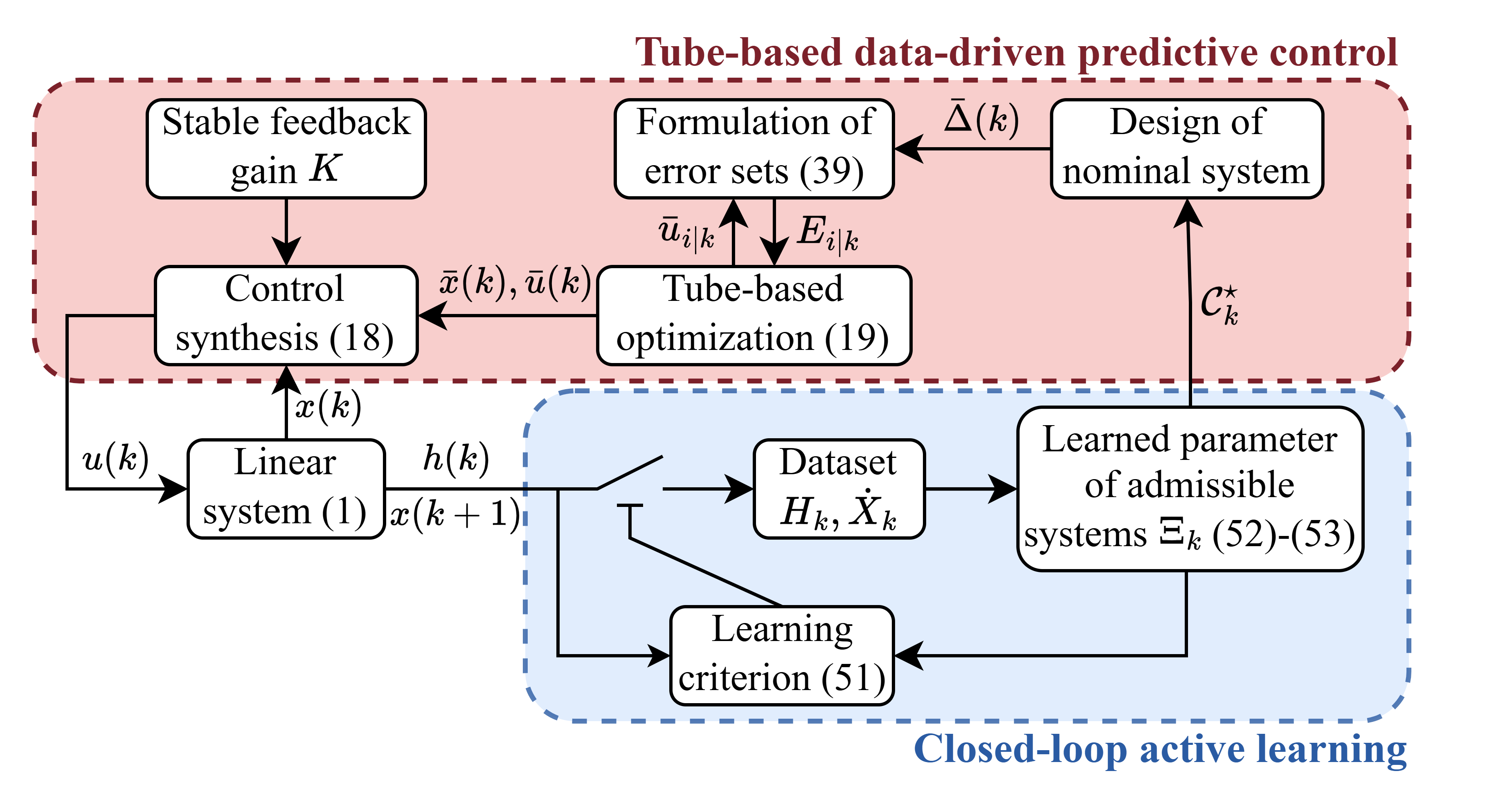
Figure 1: Schematic diagram of the proposed ATDPC schemes.

5.1 Design of Error Set and Terminal Constraint Set

In this subsection, we first introduce the design of error set $E_{i|k}$. We summarize the boundedness and other properties of the error set. Additionally, we present the design of the terminal constraint set $\mathcal{X}_{T}$ based on the bounded error set.

Based on (1), (17), and (18), we can derive the dynamics of the error as

$$e(k+1)=\Delta_{r}\begin{bmatrix}I\\[2.0pt] K\end{bmatrix}e(k)+(\Delta_{r}-\bar{\Delta}(k))\begin{bmatrix}\bar{x}(k)\\[2.0pt] \bar{u}(k)\end{bmatrix}+w(k).$$ (38)

Note that it is hard to predict the error since $\Delta_{r}$ and $w(t)$ are not available. The set $E_{i|k}$ that characterize all reachable errors, however, can be analyzed given that $\Delta_{r}\in\mathcal{C}^{\star}_{k}$ and $w(t)\!\in\!\mathcal{W}$. Suppose that $e(k)$ is available. Then $E_{i|k},i\geq 1$ can be computed by

$$E_{i+1|k}:=\left\{\Delta\begin{bmatrix}I\\ K\end{bmatrix}e+v\ \big{|}\ \Delta\!\in\!\mathcal{C}_{k}^{\star},e\!\in\!E_{i|k},v\!\in\!V_{k}\right\}$$ (39)

where

$$V_{k}\!:=\!\left\{(\Delta\!-\!\bar{\Delta}(k))\!\begin{bmatrix}\bar{x}\\ \bar{u}\end{bmatrix}\!+\!w\ \!\big{|}\!\ \Delta\!\in\!\mathcal{C}_{k}^{\star},\bar{x}\!\in\!\mathcal{X},\bar{u}\!\in\!\mathcal{U},w\!\in\!\mathcal{W}\right\}.$$

Note that the solution of (19) relates closely to the error set and the performance of the ATDPC can only be guaranteed if the error is bounded. Before we further investigate the error set, a general property relating to the inclusion relationship between two matrix ellipsoids is first introduced.

Lemma 5.21.

Let $\mathcal{E}$ and $\mathcal{E}^{\prime}$ be matrix ellipsoids. Then the relationship $\left\{Z-Z^{\prime}_{c}\ |\ Z\in\mathcal{E}^{\prime}\right\}\subseteq\left\{Z-Z_{c}\ |\ Z\in\mathcal{E}\right\}$ holds if $\mathcal{E}^{\prime}\subseteq\mathcal{E}$, where $Z_{c}$ and $Z^{\prime}_{c}$ are the centers of $\mathcal{E}$ and $\mathcal{E}^{\prime}$, respectively.

Proof 5.22.

For simplicity, we denote $\left\{Z-Z^{\prime}_{c}\ |\ Z\in\mathcal{E}^{\prime}\right\}$ by $\mathcal{S}^{\prime}$ and $\left\{Z-Z_{c}\ |\ Z\in\mathcal{E}\right\}$ by $\mathcal{S}$. Suppose that the conformable matrices ${M,N,M^{\prime},N^{\prime}}\succ 0$. Then, without loss of generality, we assume

$$\begin{split}\mathcal{E}&:=\left\{{Z\ |\ (Z-Z_{c})^{\top}M(Z-Z_{c})\preceq N}\right\},\\[2.0pt] \mathcal{E}^{\prime}&:=\left\{{Z\ |\ (Z-Z_{c}^{\prime})^{\top}M^{\prime}(Z-Z_{c}^{\prime})\preceq N^{\prime}}\right\}.\end{split}$$

Let $z:={Z-Z_{c}}$, $d:={Z_{c}^{\prime}-Z_{c}}$, then standard computations reformulate $\mathcal{E},\mathcal{E}^{\prime},\mathcal{S}$, and $\mathcal{S}^{\prime}$ as

$$\begin{split}\mathcal{E}&=\left\{{z}+Z_{c}\ |\ z^{\top}{M}z\preceq{N}\right\},\\[2.0pt] \mathcal{E}^{\prime}&=\left\{{z}+Z_{c}\ |\ (z-d)^{\top}{M^{\prime}}(z-d)\preceq{N^{\prime}}\right\},\\[2.0pt] \mathcal{S}&=\left\{z\ |\ z^{\top}{M}z\preceq{N}\right\},\\[2.0pt] \mathcal{S}^{\prime}&=\left\{z\ |\ z^{\top}{M^{\prime}}z\preceq{N^{\prime}}\right\}.\end{split}$$

Recall that $\mathcal{E}^{\prime}\subseteq\mathcal{E}$. Then we have

$$\begin{bmatrix}I\\ z\end{bmatrix}^{\top}\begin{bmatrix}N&0\\ 0&-M\end{bmatrix}\begin{bmatrix}I\\ z\end{bmatrix}\succeq 0$$ (40)

holds for all $z$ with

$$\begin{bmatrix}I\\ z\end{bmatrix}^{\top}\begin{bmatrix}N^{\prime}-d^{\top}{M^{\prime}}d&d^{\top}{M^{\prime}}\\ {M^{\prime}}d&-M^{\prime}\end{bmatrix}\begin{bmatrix}I\\ z\end{bmatrix}\succeq 0.$$ (41)

Note that if we let $z=d$, the left hand of (41) is equivalent to $N^{\prime}\succ 0$, which verifies the Slater condition. Then, Lemma 2 asserts that there exists a scalar $\alpha\geq 0$ such that

$$\begin{bmatrix}{N-\alpha N^{\prime}}+\alpha d^{\top}{M^{\prime}}d&-\alpha d^{\top}{M^{\prime}}\\[2.0pt] -\alpha{M^{\prime}}d&\alpha{M^{\prime}}-{M}\end{bmatrix}\succeq 0.$$ (42)

By invoking [59, Theorem 1.19], there exists a matrix ${L}$ such that

$$-\alpha d^{\top}{M^{\prime}}={L}(\alpha{M^{\prime}}-{M}).$$ (43)

Furthermore, [59, Theorem 1.20] affirms that

$${N-\alpha N^{\prime}}+\alpha d^{\top}{M^{\prime}}d-\alpha d^{\top}{M^{\prime}}(\alpha{M^{\prime}}-{M})^{\dagger}\alpha{M^{\prime}}d\succeq 0$$ (44)

where $\dagger$ denotes the generalized inverse of the matrix. Note that $\alpha\!\neq 0$; otherwise the second diagonal block of (42) equals to $-{M}$, which is a negative definite matrix and contradicts (42). Note that (44) is equivalent to

$$\begin{split}&{N-\alpha N^{\prime}}+\alpha d^{\top}{M^{\prime}}(\alpha M^{\prime})^{-1}(\alpha d^{\top}{M^{\prime}})^{\top}\\ &-\alpha d^{\top}{M^{\prime}}(\alpha{M^{\prime}}-{M})^{\dagger}\alpha{M^{\prime}}d\succeq 0.\end{split}$$ (45)

By using (43) to eliminate the term $\alpha d^{\top}{M^{\prime}}$, (45) can be written as

$$\begin{split}&{N-\alpha N^{\prime}}+{L}(\alpha{M^{\prime}}-{M})(\alpha M^{\prime})^{-1}(\alpha{M^{\prime}}-{M}){L}^{\top}\\ &-{L}(\alpha{M^{\prime}}-{M})(\alpha{M^{\prime}}-{M})^{\dagger}(\alpha{M^{\prime}}-{M}){L}^{\top}\succeq 0.\end{split}$$ (46)

Also note that

$$\begin{split}&(\alpha{M^{\prime}}-{M})(\alpha M^{\prime})^{-1}(\alpha{M^{\prime}}-{M})\\ &=(\alpha{M^{\prime}}-{M})-M+M(\alpha M^{\prime})^{-1}M,\\ &(\alpha{M^{\prime}}-{M})(\alpha{M^{\prime}}-{M})^{\dagger}(\alpha{M^{\prime}}-{M})=(\alpha{M^{\prime}}-{M}).\end{split}$$

Then, (46) is equivalent to

$${N-\alpha N^{\prime}}-{L(M-M(\alpha M^{\prime})^{-1}M)L^{\top}}\succeq 0.$$ (47)

Note that we have $\alpha{M^{\prime}}-{M}\succeq 0$ from (42). By standard Schur complement argument, ${M-M(\alpha M^{\prime})^{-1}M}\!\succeq\!0$ can be obtained, which implies ${N-\alpha N^{\prime}}\!\succeq\!0$. Now, we conclude that

$$\begin{bmatrix}{N-\alpha N^{\prime}}&0\\[2.0pt] 0&\alpha{M^{\prime}}-{M}\end{bmatrix}\succeq 0,$$ (48)

which proves the lemma by invoking Lemma 2.

With Lemma 5.21, several useful properties of the error set can be summarized in the following lemma.

Lemma 5.23.

For dynamic nominal system (17), if there exist a feedback gain $K$ and a matrix $P\succ 0$ such that

$$(\Delta[I\ K^{\top}]^{\top})^{\top}P(\Delta[I\ K^{\top}]^{\top})-P\prec 0,\ \forall\Delta\in\mathcal{C}^{\star}_{0},$$ (49)

and $e(0)$ is bounded, then the following statements hold.

1. there exists a bounded set $E_{0}$ such that $E_{i|0}\subseteq E_{0},\forall i\in\mathbb{Z}_{\geq 0}$.

2. it holds that $E_{i|k+1}\subseteq E_{i+1|k}$ if $\mathcal{C}_{k+1}^{\star}\subseteq\mathcal{C}_{k}^{\star}$, $\forall k\in\mathbb{Z}_{\geq t_{0}},i\in\mathbb{Z}_{\geq 0}$.

Proof 5.24.

For the first statement, we consider $E_{i|0}^{0}$ and $E_{i|0}^{1}$, where $E_{i|0}^{0}$ equals to $E_{i|0}$ when $e(0)=0$ and $E_{i|0}^{1}$ characterizes the propagation of $e(0)$. Let $E_{i|0}^{0}=\{0\}$ and $E_{i|0}^{1}=\{e(0)\}$ when $i=0$. For $i\in\mathbb{Z}_{\geq 1}$, $E_{i|0}^{0}$ and $E_{i|0}^{1}$ can be computed by

$$\begin{split}E_{i|0}^{0}&=\left\{\Delta\!\begin{bmatrix}I\\ K\end{bmatrix}e+v\ \!\big{|}\!\ \Delta\in\mathcal{C}_{0}^{\star},e\in E_{i-1|0}^{0},v\in V_{0}\right\},\\ E_{i|0}^{1}&=\left\{\Delta\!\begin{bmatrix}I\\ K\end{bmatrix}e\ \!\big{|}\!\ \Delta\in\mathcal{C}_{0}^{\star},e\in E_{i-1|0}^{1}\right\}.\end{split}$$

It can be easily verified that $E_{i|k}=E_{i|k}^{0}\oplus E_{i|k}^{1},\forall i\in\mathbb{Z}_{\geq 0}$. Thus, the existence of $E_{0}$ can be guaranteed if there exist bounded sets $E_{0}^{0}$ and $E_{0}^{1}$ such that $E_{i|0}^{0}\subseteq E_{0}^{0},E_{i|0}^{1}\subseteq E_{0}^{1},\forall i\in\mathbb{Z}_{\geq 0}$. Given the assumption (49) and the fact that $E_{i|0}^{0}=\{0\}$, the existence of such $E_{0}^{0}$ follows directly from [51, Lemma 5]. Additionally, by using (49) and invoking [60, Theorem 8], there exist $\eta_{1},\eta_{2}>0$ such that $\|e_{i}\|_{2}\!<\!\eta_{1}e^{-\eta_{2}i}\|e(0)\|_{2},\forall e_{i}\!\in\!E_{i|0}^{0},i\in\mathbb{Z}_{\geq 1}$. Note that since $e(0)$ is bounded, we can also conclude that there exists an $E_{0}^{1}$ such that $E_{i|0}^{1}\!\subseteq\!E_{0}^{1},\forall i\!\in\!\mathbb{Z}_{\geq 0}$.

For the second statement, we will prove it by mathematical induction (MI). When $i=0$, we have $E_{0|k+1}=\{e(k+1)\}=\{\Delta_{r}[I\ K^{\top}]^{\top}\!e(k)+(\Delta_{r}-\bar{\Delta}(k))[\bar{x}(k)^{\top}\ \bar{u}(k)^{\top}]^{\top}\!+w(k)\},\forall k\in\mathbb{Z}_{\geq t_{0}}$, where $\Delta_{r}\!\in\!\mathcal{C}_{k}^{\star},\bar{x}(k)\!\in\!\mathcal{X},\bar{u}(k)\!\in\!\mathcal{U},w(k)\!\in\!\mathcal{W}$. By the definition of $E_{i|k}$, we can easily conclude that $E_{0|k+1}\subseteq E_{1|k}$. Furthermore, assume that the statement holds for all $k\!\in\!\mathbb{Z}_{\geq t_{0}},i\!\in\!\mathbb{Z}_{[0,j-1]}$. Then, for $i=j$, we have

$$\begin{split}E_{j|k+1}\!&=\!\left\{\Delta\!\begin{bmatrix}I\\ K\end{bmatrix}\!e\!+\!v\!\ \big{|}\!\ \Delta\!\in\!\mathcal{C}_{k+1}^{\star},e\!\in\!E_{j-1|k+1},v\!\in\!V_{k+1}\right\},\!\\ E_{j+1|k}\!&=\!\left\{\Delta\!\begin{bmatrix}I\\ K\end{bmatrix}\!e\!+\!v\!\ \big{|}\!\ \Delta\!\in\!\mathcal{C}_{k}^{\star},e\!\in\!E_{j|k},v\!\in\!V_{k}\right\}.\end{split}$$

Note that $\mathcal{C}_{k+1}^{\star}\subseteq\mathcal{C}_{k}^{\star}$ is guaranteed by (53). By letting $\mathcal{E}=\mathcal{C}_{k}^{\star}$, $\mathcal{E}^{\prime}\!=\mathcal{C}_{k+1}^{\star}$, $Z_{c}=\bar{\Delta}(k)$, and $Z_{c}^{\prime}\!=\bar{\Delta}(k+1)$, we have $V_{k+1}\subseteq V_{k}$ by invoking Lemma 5.21. Besides, $E_{j-1|k+1}\subseteq E_{j|k}$ can be obtained from the MI assumption. We can now conclude that the second statement holds for all $k\in\mathbb{Z}_{\geq t_{0}},i\in\mathbb{Z}_{\geq 0}$.

With the bounded reachable error set $E_{0}$ and the definition of the terminal constraint $\mathcal{X}_{T}$, the parameter $L_{T}$ of the terminal constraint for any given matrices $P_{T}$ and $K$ can be obtained by solving an optimization problem:

$$\begin{split}&\max_{L_{T}}\ L_{T}\\ &\ \text{s.t.}\ Kx\in\mathcal{U}\ominus KE_{0},\ \forall x\in\{x\ |\ x^{\top}P_{T}x\leq L_{T}\}.\end{split}$$ (50)

By revisiting the formulation of $E_{i|k}$ in (39) and invoking Lemma 5.21, we can conclude that the size of $E_{i|k}$ correlates with $\mathcal{C}_{k}^{\star}$. Recall that a smaller $E_{i|k}$ will enable a less conservative solution for (19) and result in a more desirable control performance. Besides, the second statement of Lemma 5.23 asserts that the contraction of the error set can be guaranteed if the ASE is contracting. This motivates the following subsection, in which we design a closed-loop active learning strategy to learn a contracting ASE by further exploring closed-loop data samples.

5.2 Closed-Loop Active Learning for Contracting ASEs

When the controller is employed, the inputs are determined by (18) and cannot be designed freely. Therefore, an active learning strategy is proposed in this section to learn the contracting ASE by actively selecting closed-loop data samples. In addition, the design of dynamical nominal system is also discussed.

Suppose that the dataset we obtained in the open-loop stage at $t_{0}$ is denoted by $(H_{t_{0}},\dot{X}_{t_{0}},\Lambda_{t_{0}})$. We denote $\Xi(H_{t_{0}},\dot{X}_{t_{0}},\Lambda_{t_{0}})$ by $\Xi_{0}$ for brevity. Then, for $k\geq t_{0}+1$, the active learning criterion is designed as

$$\xi(h(k-1),x(k))-\alpha\Xi_{k-1}\succeq 0.$$ (51)

The corresponding learning strategy is presented as follows

$$\begin{split}H_{k}&=\left\{\begin{array}[]{lc}H_{k-1},\ \text{if $\exists\alpha\geq 0$ such that \eqref{eq:ETL_scheduler} holds}\\[2.0pt] [H_{k-1}\ |\ h(k-1)],\ \text{otherwise}\\ \end{array}\right.\\ \dot{X}_{k}&=\left\{\begin{array}[]{lc}\dot{X}_{k-1},\ \text{if $\exists\alpha\geq 0$ such that \eqref{eq:ETL_scheduler} holds}\\[2.0pt] [\dot{X}_{k-1}\ |\ x(k)],\ \text{otherwise}\\ \end{array}\right.\\ \Xi_{k}&=\left\{\begin{array}[]{lc}\Xi_{k-1},\ \text{if $\exists\alpha\geq 0$ such that \eqref{eq:ETL_scheduler} holds}\\[2.0pt] \Xi(H_{k},\dot{X}_{k},\Lambda_{s}),\ \text{otherwise}\\ \end{array}\right.\end{split}$$ (52)

where $\Lambda_{s}$ is the solution of the convex optimization problem:

$$\begin{split}&\max_{\Lambda_{s}\in\mathcal{D}_{\text{col}(H_{k})},\sigma\geq 0}\sigma\\ &\ \text{s.t. }\Xi_{k-1}-\Xi(H_{k},\dot{X}_{k},\Lambda_{s})\succeq\sigma\text{diag}(I_{n_{x}},0).\end{split}$$ (53)

For compactness, we also denote

$$\mathcal{C}^{\star}_{k}:=\bigg{\{}\Delta\ \Big{|}\ \begin{bmatrix}I\\[2.0pt] \Delta^{\top}\end{bmatrix}^{\top}\Xi_{k}\begin{bmatrix}I\\[2.0pt] \Delta^{\top}\end{bmatrix}\succeq 0\bigg{\}},k\in\mathbb{Z}_{\geq t_{0}}.$$

The learning strategy in (53) is designed to gradually construct an contracting ASE with a small size. The constraint $\sigma\geq 0$ ensures that $\Xi_{k-1}-\Xi_{k}\succeq 0$, which implies the contraction of the ASE, namely, $\mathcal{C}^{\star}_{k}\subseteq\mathcal{C}^{\star}_{k-1}$, by invoking Lemma 2. Besides, the objective function $\sigma$ is introduced to learn a relatively small $\mathcal{C}^{\star}_{k}$ because a larger $\sigma$ implies a smaller upper bound on the volume of $\mathcal{C}^{\star}_{k}$ according to Lemmas 1-2. Note that the execution of (53) could be resource-consuming. Therefore, we introduce the learning criterion in (51) to mitigate this issue by only triggering (53) when an informative data sample is detected. An intuitive interpretation of (51) is that if all admissible systems in the current ASE are compatible with the latest data sample, the learning criterion will not be satisfied according to Lemma 2. Therefore, it is unnecessary to trigger the learning strategy in (53) because the latest data sample cannot exclude any admissible system in the ASE. To further illustrate the rationale of the proposed active learning strategy, we investigate the influence of the uncollected data sample to the optimization problem (53). For convenience, we define $H_{k}^{+}:=[H_{k-1}\ h(k-1)]$ and $\dot{X}_{k}^{+}:=[\dot{X}_{k-1}\ x(k)]$, which represent the collected dataset without (51). In this condition, the optimization problem can be accordingly formulated as

$$\begin{split}&\max_{\Lambda_{s}\in\mathcal{D}_{\text{col}(H_{k}^{+})},\sigma\geq 0}\sigma\\ &\ \text{s.t. }\Xi_{k-1}-\Xi(H_{k}^{+},\dot{X}_{k}^{+},\Lambda_{s})\succeq\sigma\text{diag}(I_{n_{x}},0).\end{split}$$ (54)

Suppose that the optimal value of $\sigma$ solved by (53) is $\sigma^{\star}(k)$ and the one solved by (54) is $\sigma^{+}(k)$. Then, properties of the proposed active learning strategy are summarized in the following theorem.

Theorem 5.25.

For ATDPC with learning strategy (52) and the learning criterion (51), the following statements hold:

1. the optimization problem (53) is feasible for all $k\in\mathbb{Z}_{\geq t_{0}+1}$.

2. for $k\geq t_{0}+1$, if there exist $\alpha\geq 0$ such that the learning criterion (51) holds, we have $\sigma^{\star}(k)\geq\sigma^{+}(k)$.

Proof 5.26.

We prove the first statement by MI. Recall that $\Xi_{0}=\Xi(H_{0},\dot{X}_{0},\Lambda_{0})$. For $k=t_{0}+1$, if there exists $\alpha\geq 0$ such that (51) is satisfied, we have $H_{1}=H_{0}$ and $\dot{X}_{1}=\dot{X}_{0}$. It can be verified that $\Lambda_{s}=\Lambda_{0}$ and $\sigma=0$ is a feasible solution to the optimization problem (53). On the other hand, if (51) is not satisfied, the constraint can still be satisfied by letting $\Lambda_{s}=\text{diag}(\Lambda_{0},0)$ and $\sigma=0$. For $k\geq t_{0}+2$, we assume that there exists $\Lambda_{k-1}$ such that

$$\Xi_{k-2}-\Xi(H_{k-1},\dot{X}_{k-1},\Lambda_{k-1})\succeq 0$$ (55)

is satisfied. Then the feasibility of (53) can be analyzed following a similar line of argument to the case of $k=1$.

For the second statement, we denote $\text{col}(H_{k}^{+})$ by $n$ for compactness. Suppose that $\Lambda^{+}=\text{diag}(\lambda_{1},\lambda_{2},\dots,\lambda_{n})$ is a solution corresponding to the optimal value $\sigma^{+}(k)$ in optimization problem (54). We have

$$\Xi_{k-1}\!-\!\sum\limits_{i=1}^{n}\lambda_{i}\xi((H_{k}^{+})_{[i]},({\dot{X}}_{k}^{+})_{[i]})\succeq\sigma^{+}(k)\text{diag}(I_{n_{x}},0)$$ (56)

according to (54). Besides, we also have

$$\xi((H_{k}^{+})_{[n]},({\dot{X}}_{k}^{+})_{[n]})-\alpha\Xi_{k-1}\succeq 0$$ (57)

according to (51). Based on the assumption and the constraint in (54), we have $\alpha\geq 0$ and $\lambda_{n}\geq 0$.

To prove the statement, we first consider a special condition $\alpha=0$. By invoking (57), we have $\xi((H_{k}^{+})_{[n]},({\dot{X}}_{k}^{+})_{[n]})\succeq 0$ when $\alpha=0$. Thus, we can obtain

$$\Xi_{k-1}\!-\!\sum\limits_{i=1}^{n-1}\lambda_{i}\xi((H_{k}^{+})_{[i]},({\dot{X}}_{k}^{+})_{[i]})\succeq\sigma^{+}(k)\text{diag}(I_{n_{x}},0),$$ (58)

which proves that the constraint in (53) is satisfied by letting $\Lambda_{s}=\text{diag}(\lambda_{1},\lambda_{2},\dots,\lambda_{n-1})$ and $\sigma=\sigma^{+}(k)$. Therefore, we have $\sigma^{\star}(k)\geq\sigma^{+}(k)$ when $\alpha=0$.

Next, for the case of $\alpha>0$, by eliminating the term $\Xi_{k-1}$ using (56) and (57), we can obtain

$$\begin{split}&(1-\alpha\lambda_{n})\xi((H_{k}^{+})_{[n]},({\dot{X}}_{k}^{+})_{[n]})\\ &\succeq\alpha\sum\limits_{i=1}^{n-1}\lambda_{i}\xi((H_{k}^{+})_{[i]},({\dot{X}}_{k}^{+})_{[i]})+\alpha\sigma^{+}(k)\text{diag}(I_{n_{x}},0).\end{split}$$ (59)

By pre- and postmultiplication of the right hand of (59) with $[I\ \Delta_{r}]$ and $[I\ \Delta_{r}]^{\top}$, it can be concluded that

$$(1-\alpha\lambda_{n})\begin{bmatrix}I\\[2.0pt] \Delta_{r}^{\top}\end{bmatrix}^{\top}\!\xi((H_{k}^{+})_{[n]},({\dot{X}}_{k}^{+})_{[n]})\begin{bmatrix}I\\[2.0pt] \Delta_{r}^{\top}\end{bmatrix}\succ 0.$$

according to (7), which implies $1-\alpha\lambda_{n}>0$. Since $\alpha>0$ and $\lambda_{n}\geq 0$, we have $0<1-\alpha\lambda_{n}\leq 1$. Let $\tau:=1-\alpha\lambda_{n}$. Then, by eliminating the term $\xi((H_{k}^{+})_{[n]},({\dot{X}}_{k}^{+})_{[n]})$ using (56) and (57), we obtain

$$\tau\Xi_{k-1}-\sum\limits_{i=1}^{n-1}\lambda_{i}\xi((H_{k}^{+})_{[i]},({\dot{X}}_{k}^{+})_{[i]})\succeq\sigma^{+}(k)\text{diag}(I_{n_{x}},0),$$

which is equivalent to

$$\Xi_{k-1}-\sum\limits_{i=1}^{n-1}\frac{\lambda_{i}}{\tau}\xi((H_{k}^{+})_{[i]},({\dot{X}}_{k}^{+})_{[i]})\succeq\frac{\sigma^{+}(k)}{\tau}\text{diag}(I_{n_{x}},0).$$

Note that $\text{diag}(\lambda_{1},\lambda_{2},\dots,\lambda_{n})\in\mathcal{D}_{n}$, $\tau\in(0,1]$, and $\sigma^{+}\geq 0$. It follows directly that the constraint in (53) is satisfied when $\Lambda_{s}=\text{diag}(\lambda_{1}/\tau,\lambda_{2}/\tau,\dots,\lambda_{n-1}/\tau)$ and $\sigma=\sigma^{+}(k)/\tau$. Thus, we have $\sigma^{\star}(k)\geq\sigma^{+}(k)/\tau\geq\sigma^{+}(k)$.

In Theorem 5.25, we show that (53) is feasible for $k\in\mathbb{Z}_{\geq t_{0}+1}$. Recall that (53) is a convex problem. It can be solved by using well-known CVX toolbox [61]. In addition, we also show that the inclusion of data sample that does not meet the learning criterion (51) will not enable a larger $\sigma$. In other words, the inclusion of unselected data samples cannot lead to a smaller ASE, which does not comply to the learning algorithm. Thus, the proposed active learning strategy is able to reduce the learning frequency while maintaining the learning performance.

5.3 Recursive Feasibility and Stability of ATDPC

In this section, we aim to show that the ATDPC is recursively feasible and could stabilize the true system with the proposed closed-loop active learning strategy. To this end, a lemma is introduced first to bribluee ATDPC with the proposed active learning strategy in Section 4.

Lemma 5.27.

For system (1) and its ASE $\mathcal{C}(H,\dot{X},\Lambda)$, assume that the generalized Slater condition (5) holds for $\Xi(H,\dot{X},\Lambda)$ and some $\bar{Z}\in\mathbb{R}^{(n_{x}+n_{u})\times n_{x}}$, then there exist matrices $K$ and $P_{T}$ such that

$$V_{f}(Ax+Bu)-V_{f}(x)\leq-l(x,u)$$ (60)

for $\forall x\in\mathcal{X}_{T}$, $\forall{\Delta}\in\mathcal{C}(H,\dot{X},\Lambda)$, where $u=Kx$, if and only if there exists matrix $Y\in\mathbb{R}^{n_{x}\times n_{x}}$, $Y=Y^{\top}\succ 0$, $L\in\mathbb{R}^{n_{u}\times n_{x}}$, and scalar $\alpha\geq 0$ such that

$$\begin{bmatrix}R^{-1}&L\\[4.0pt] L^{\top}&Y-YQY\\ \end{bmatrix}\succ 0$$ (61)

and (62) hold.

$$\begin{bmatrix}\begin{array}[]{ccc:cc:c}Y&0&0&0&0&0\\ 0&0&0&0&Y&0\\ 0&0&0&0&L&0\\ \hdashline 0&0&0&\raisebox{0.0pt}[10.0pt]{$R^{-1}$}&L&0\\ 0&Y^{\top}&L^{\top}&L^{\top}&Y&Y\\ \hdashline 0&0&0&0&Y&\raisebox{0.0pt}[10.0pt]{$Q^{-1}$}\\ \end{array}\end{bmatrix}-\alpha\begin{bmatrix}\Xi(H,\dot{X},\Lambda)&0\\ 0&0_{2n_{x}+n_{u}}\end{bmatrix}\succeq 0$$ (62)

$$\begin{bmatrix}\begin{array}[]{ccc:cc}Y&0&0&0&0\\ 0&0&0&0&Y\\ 0&0&0&0&L\\ \hdashline 0&0&0&\raisebox{0.0pt}[10.0pt]{$R^{-1}$}&L\\ 0&Y^{\top}&L^{\top}&L^{\top}&Y-YQY\\ \end{array}\end{bmatrix}-\alpha\begin{bmatrix}\Xi(H,\dot{X},\Lambda)&0\\ 0&0_{n_{x}+n_{u}}\end{bmatrix}\succeq 0$$ (63)

Proof 5.28.

For the “if” part, suppose that there exist matrices $Y=Y^{\top}\succ 0$, $L$ and scalar $\alpha\geq 0$ satisfying (61) and (62). By making use of the fact that $R\succ 0$ and computing the Schur complement of (61) with respect to $R^{-1}$, we get $G_{s}\succ 0$ where $G_{s}:=Y-YQY-L^{\top}RL.$ Next, since $Q\succ 0$, the Schur complement of (62) with respect to $R^{-1}$ implies that (62) is equivalent to (63). Then, note that the second diagonal block of (63) is positive definite. By computing the Schur complement of (63) with respect to the second diagonal block, we obtain that

$$\underbrace{\begin{bmatrix}\begin{array}[]{c:c}Y&0\\ \hdashline 0&\raisebox{0.0pt}[20.0pt]{$-\begin{bmatrix}Y\\ L\end{bmatrix}G_{s}^{-1}\begin{bmatrix}Y\\ L\end{bmatrix}^{\top}$}\end{array}\end{bmatrix}}_{:=M_{s}}-\alpha\Xi(H,\dot{X},\Lambda)\succeq 0.$$ (64)

By invoking Lemma 2, (64) implies

$$\begin{bmatrix}I\\[4.0pt] \Delta^{\top}\end{bmatrix}^{\top}M_{s}\begin{bmatrix}I\\[4.0pt] \Delta^{\top}\end{bmatrix}\succeq 0,\ \forall\Delta\in\mathcal{C}(H,\dot{X},\Lambda),$$ (65)

which is equivalent to

$$Y\!-\!(AY\!+\!BL)G_{s}^{-1}(AY\!+\!BL)^{\top}\succeq 0,\forall\Delta\!\in\!\mathcal{C}(H,\dot{X},\Lambda).$$ (66)

Recall that $G_{s}\succ 0$. Then, by standard Schur complement argument, (65) implies that

$$\begin{bmatrix}Y-YQY-L^{\top}RL&(AY+BL)^{\top}\\[4.0pt] AY+BL&Y\end{bmatrix}\succeq 0$$ (67)

holds for all $\Delta\in\mathcal{C}(H,\dot{X},\Lambda)$. By computing the Schur complement of (67) with respect to the second diagonal block, we can obtain that

$$Y-(AY+BL)^{\top}Y^{-1}(AY+BL)-YQY-L^{\top}RL\succeq 0$$ (68)

holds for $\forall\Delta\in\mathcal{C}$. By letting $P_{T}=Y^{-1}$ and $K=LP_{T}$,

$$P_{T}-(A+BK)^{\top}P_{T}(A+BK)\succeq Q+K^{\top}RK$$ (69)

holds for all $\Delta\in\mathcal{C}(H,\dot{X},\Lambda)$. Finally, we can conclude that (60) holds for all $x\in\mathbb{R}^{n_{x}}$ (which includes $\mathcal{X}_{T}$) and ${\Delta}\in\mathcal{C}$.

For “only if” part, since (60) holds for all $x\in\mathcal{X}_{T}$, we have

$$\begin{bmatrix}1\\[2.0pt] x\end{bmatrix}^{\top}\begin{bmatrix}0&0\\[2.0pt] 0&P_{T}-{A}_{K}^{\top}P_{T}{A}_{K}-Q-K^{\top}RK\end{bmatrix}\begin{bmatrix}1\\[2.0pt] x\end{bmatrix}\succeq 0$$ (70)

for $\forall\Delta\in\mathcal{C}$ and $\forall x\in\mathbb{R}^{n_{x}}$ with

$$\begin{bmatrix}1\\[2.0pt] x\end{bmatrix}^{\top}\begin{bmatrix}L_{T}&0\\[2.0pt] 0&-P_{T}\end{bmatrix}\begin{bmatrix}1\\[2.0pt] x\end{bmatrix}\succeq 0$$ (71)

where $A_{K}:=A+BK$. Note that when $x$ is a zero vector, (71) is positive since $L_{T}>0$. Then Lemma 2 asserts that the claim we proposed holds if and only if there exists $\beta\geq 0$ such that

$$\begin{bmatrix}0&0\\[2.0pt] 0&P_{T}-{A}_{K}^{\top}P_{T}{A}_{K}-Q-K^{\top}RK\end{bmatrix}-\beta\begin{bmatrix}L_{T}&0\\[2.0pt] 0&-P_{T}\end{bmatrix}\succeq 0.$$ (72)

Recall that by $L_{T}>0$, we have (72) holds if and only if $\beta=0$ and

$$P_{T}-{A}_{K}^{\top}P_{T}{A}_{K}-Q-K^{\top}RK\succeq 0$$ (73)

for all $\Delta\in\mathcal{C}$. This statement is equivalent to (69) and also proves (61) and (62) by letting $Y\!=\!P_{T}^{-1}$ and $L\!=\!KY$.

Remark 5.29.

The linear matrix inequalities (LMIs) (61) and (62) in Lemma 5.27 provides the sufficient condition that there exists a controller $u=Kx$ such that (60) holds for $\forall x\in\mathcal{X}_{T},\Delta\in\mathcal{C}$. Moreover, (60) also implies

$$V_{f}(Ax+Bu)-V_{f}(x)\!\leq\!0,\forall x\!\in\mathcal{X}_{T},\Delta\!\in\mathcal{C}(H,\dot{X},\Lambda),$$ (74)

from which we can conclude that there exists a controller $u=Kx$ such that

$$V_{f}(Ax+Bu)\leq L_{T},\ \forall x\in\mathcal{X}_{T},\Delta\in\mathcal{C}(H,\dot{X},\Lambda).$$

As such, Lemma 5.27 provides a sufficient condition for the existence of the controller $u=Kx$ such that $Ax+Bu\in\mathcal{X}_{T},\forall x\in\mathcal{X}_{T},{\Delta}\in\mathcal{C}(H,\dot{X},\Lambda)$.

Recall that in the open-loop stage, we obtained an ASE denoted by $\mathcal{C}^{\star}_{0}$. Then by considering the $\mathcal{C}^{\star}_{0}$ in the context of Lemma 5.27, we can set matrices $P_{T}$ and $K$ in ATDPC as $P_{T}=Y^{-1}$ and $K=LP_{T}$ respectively, where $Y$ and $L$ are matrices such that (61) and (62) hold. Additionally, the conclusions drawn in Lemma 5.27 and Remark 5.29 both hold for all systems in $\mathcal{C}^{\star}_{0}$ with $P_{T}$ and $K$, and the assumption (49) in Lemma 5.21 holds.

Now, we are in a position to discuss the recursive feasibility and stability of ATDPC. To this end, by making use of Lemmas 5.23, 5.27 and Remark 5.29, the recursive feasibility and stability are analyzed in the following theorem.

Theorem 5.30.

For system (1) and the ASE $\mathcal{C}^{\star}_{0}$, assume that the generalized Slater condition (5) holds for $\Xi_{0}$ and some $\bar{Z}\in\mathbb{R}^{(n_{x}+n_{u})\times n_{x}}$. If there exist matrices $Y\in\mathbb{R}^{n_{x}\times n_{x}}$, $Y=Y^{\top}\succ 0$, $L\in\mathbb{R}^{n_{u}\times n_{x}}$, and a scalar $\alpha\geq 0$ that satisfy (61) and (62), then the following statements hold:

1. the optimization problem (19) is recursively feasible.

2. the control sequence determined by (18) and (19) manipulates the state of the true system to a bounded set.

Proof 5.31.

Given the fact that there exist matrices $Y$ and $L$ such that (61) and (62) hold, we let $P=Y^{-1}$, $K=LP$. For recursive feasibility, we first assume that it is feasible at instant $k\in\mathbb{Z}_{\geq 0}$. Then there exists an optimal control sequence $\bar{u}_{\text{seq},k}^{\star}=(\bar{u}^{\star}_{0|k},\bar{u}^{\star}_{1|k},\dots,\bar{u}^{\star}_{N-1|k})$ such that $\bar{x}_{N|k}^{\star}\in\mathcal{X}_{T}$, $\bar{u}^{\star}_{i|k}\in\mathcal{U}\ominus KE_{i|k}$, $\forall i\in\mathbb{Z}_{\geq 0}$. At instant $k+1$, we consider a control sequence $\bar{u}_{\text{seq},k+1}$ where

$$\bar{u}_{i|k+1}=\left\{\begin{array}[]{lc}\bar{u}^{\star}_{i+1|k},\ i\in\mathbb{Z}_{[0,N-2]},\\[4.0pt] K\bar{x}_{N|k}^{\star},\ i=N-1.\end{array}\right.$$ (75)

By the second statement of Lemma 5.23, $\bar{u}_{i|k+1}=\bar{u}^{\star}_{i+1|k}\in\mathcal{U}\ominus KE_{i+1|k}$ and $E_{i|k+1}\subseteq E_{i+1|k}$ for $\forall i\in\mathbb{Z}_{\geq 0}$. We conclude that $\bar{u}_{i|k+1}\in\mathcal{U}\ominus KE_{i|k+1}$ for $\forall i\in\mathbb{Z}_{[0,N-2]}$. Moreover, for $i=N-1$, since $\bar{x}_{N|k}^{\star}\in\mathcal{X}_{T}$, $\bar{u}_{N-1|k+1}$ is a feasible control input on the basis of (50). Besides, $\bar{x}_{N|k+1}\in\mathcal{X}_{T}$ can be derived by Remark 5.29. The recursive feasibility of (19) is thus proved.

For the stability of the ATDPC, we reconsider the input sequence $\bar{u}_{\text{seq},k+1}$ which is defined in (75). Suppose that the optimal solution is $\bar{u}_{\text{seq},k+1}^{\star}$. Then, we have

$$V_{s}(\bar{x}_{0|k+1},\bar{u}_{\text{seq},k+1}^{\star})\leq V_{s}(\bar{x}_{0|k+1},\bar{u}_{\text{seq},k+1}).$$ (76)

Furthermore, we have

$$\begin{split}V_{s}(\bar{x}_{0|k+1},\bar{u}_{\text{seq},k+1})\!=\!V_{s}(\bar{x}_{0|k},\bar{u}_{\text{seq},k}^{\star})-l(\bar{x}_{0|k},\bar{u}_{0|k}^{\star})+\mathcal{F}\end{split}$$ (77)

where

$$\mathcal{F}:=V_{f}(\bar{\Delta}(k)\begin{bmatrix}I\\ K\end{bmatrix})-V_{f}(\bar{x}_{N|k}^{\star})+l(\bar{x}_{N|k}^{\star},K\bar{x}_{N|k}^{\star})$$

Given that $\bar{x}_{N|k}^{\star}\in\mathcal{X}_{T}$, $\mathcal{F}\leq 0$ follows from Lemma 5.27. Thus,

$$V_{s}(\bar{x}_{0|k+1},\bar{u}_{\text{seq},k+1}^{\star})-V_{s}\bar{x}_{0|k},\bar{u}_{\text{seq},k}^{\star})\leq-l(\bar{x}_{0|k},\bar{u}_{0|k}^{\star})$$

can be obtained according to (76) and (77). With the definition of the stage cost function, we also have

$$V_{s}(\bar{x}_{0|k+1},\bar{u}_{\text{seq},k+1}^{\star})-V_{s}(\bar{x}_{0|k},\bar{u}_{\text{seq},k}^{\star})<0,\ \forall\bar{x}_{0|k}\neq 0.$$

Therefore, the nominal system is asymptotically stable for the origin. Recall that $x(k)=\bar{x}(k)+e(k)$. Since $\bar{x}(k)$ converges to the origin, the distribution of $x(k)$ depends on $e(k)$ which belongs to a bounded set by Lemma 5.23. Finally, we conclude that the true state is expected to converge to a bounded set.

Remark 5.32.

By considering the set-valued ASE, we ensure that the ATDPC stabilize the true system. Also note that the difference between the state of the true system and the dynamic nominal system belongs to the error set $E_{i|k}$, the size of which closely relates to that of $\mathcal{C}_{k}^{\star}$. Compared with the system identification approach, the proposed closed-loop active learning strategy leverages closed-loop data to learn a series of contracting $\mathcal{C}_{k}^{\star}$, which could lead to a less conservative solution for (19) and a more desirable control performance. Furthermore, it’s important to note that learning a series of contracting ASEs also ensures the feasibility and stability of the controller. Compared with the standard idenfication+model-based control approach, the proposed approach features active input design to escalate the model-learning process during the open-loop learning stage, and event-triggered data selection and model update during the closed-loop control stage to enable more precise and data-efficient understanding of the underlying controlled process.

6 Numerical Examples

In this section, we illustrate the advantage and effectiveness of our theoretical results by two numerical simulations.

6.1 Visualization of Open-Loop Active Learning

To visualize the efficiency of the proposed active learning strategy, we first consider a simple scalar system (1) with $\mathcal{A}=1$, $\mathcal{B}=1$, and $\delta=1$. Assume that the input constraint for open-loop active learning is $\mathcal{U}_{o}=\{u\ |\ \|u\|_{2}\leq 5\}$. As a comparison, under the framework of [55], we apply the input design strategies for data-driven analysis and control in [14] and [16], which are denoted by ID-PE and ID-$\alpha$PE, respectively. The ID-PE aims to select inputs online such that the full rank properties of the data matrix can be achieved. While the ID-$\alpha$PE designs an input sequence offline such that minimum singular value of the data matrix can be lower bounded. Fig. 2 illustrates the average volume of ASE obtained by ID-PE and ID-$\alpha$PE compared to those obtained by the proposed approach in a batch of 100 simulations, as the number of data samples increases from $T\!=\!2$ to $T\!=\!16$. Due to the additional consideration of the volume of ASE as an informativity metric in the design of inputs, the proposed approach consistently achieves a smaller average volume. Similarly, we can see that the proposed approach is capable of learning a small ASE volume with fewer data samples.

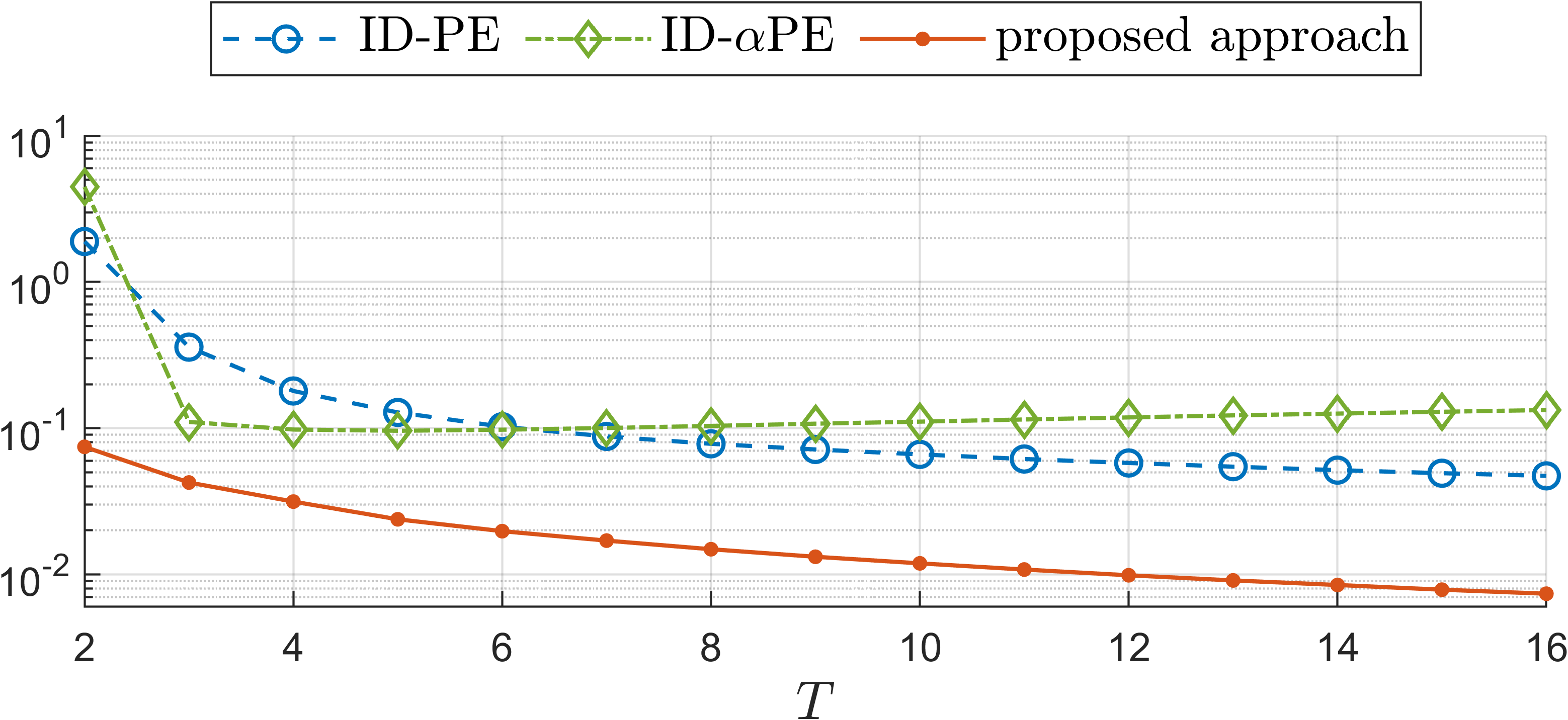
Figure 2: Volume of the ASE obtained by different input design approaches.

Additionally, we visualize the performance of these approaches by plotting the space of the learned ASEs at $T=2,4,8,16$ in Fig. 3, where the efficiency of the proposed approach in learning a small ASE can be observed more intuitively.

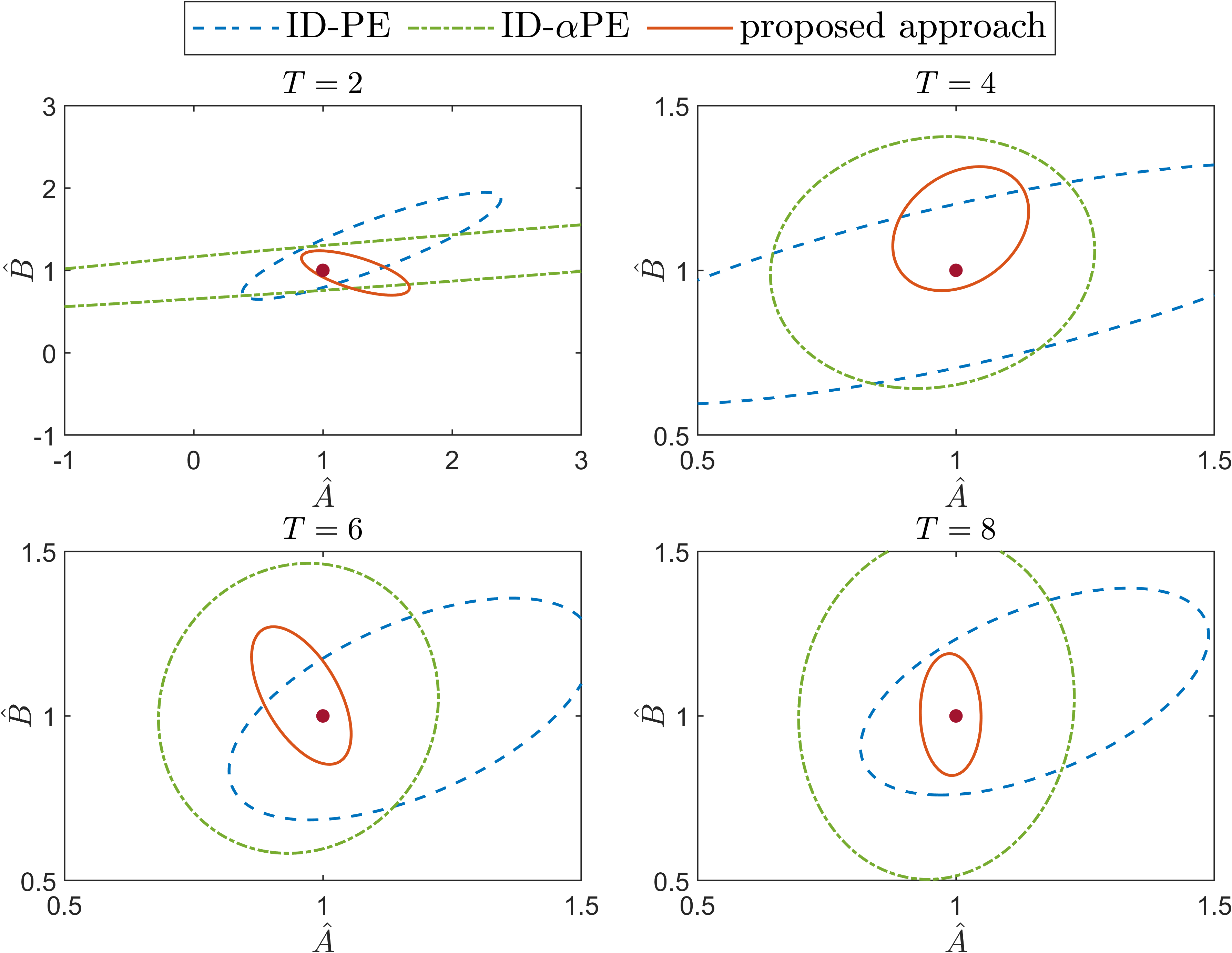
Figure 3: Space of the ASE obtained by different input design approaches. The dark brown dot represents the true system.

6.2 Illustration of Active Learning and Control

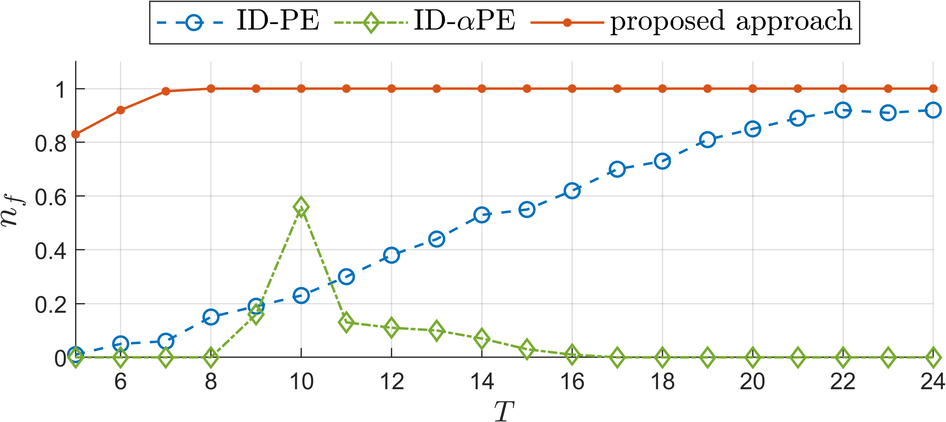
Figure 4: Ratio of feasible problems using different input design approaches.

In this section, we delve into the consideration of a more complex example to represent the learning and control performance of ATDPC. We consider system (1) with

$$\mathcal{A}=\begin{bmatrix}0.850&-0.038&-0.038\\ 0.735&0.815&1.594\\ -0.664&0.697&-0.064\end{bmatrix},\mathcal{B}=\begin{bmatrix}1.431&0.705\\ 1.62&-1.129\\ 0.913&0.369\end{bmatrix},$$

and we let $Q=I_{3}$, $R=I_{2}/10$, and $\delta=0.16$. The constraint for open-loop active learning is $\mathcal{U}_{o}\!=\!\{u\in\mathbb{R}^{2}\ |\ \|u\|_{2}\leq 2\}$. We first analyze the influence of learning strategies and number of data samples to the feasibility of ATDPC. For each number of collected data samples $T\in[5,24]$, we solve a batch of $100$ feasibility problem of ATDPC, count the number of feasible instances by $n_{f}$, and display ${n_{f}}/{100}$ for each approach in Fig. 4. The proposed approach yields better performance in terms of the feasibility compared to ID-PE and ID-$\alpha$PE. Specifically, our approach allows the design of ATDPC in a high probability ($n_{f}\geq 0.8$) when $T\geq 5$, and guarantee the feasibility ($n_{f}=1$) when $T\geq 7$. In contrast, ID-PE enables the design of ATDPC in a high probability when $T\geq 19$, and ID-$\alpha$PE only achieves a notable feasibility when $T=10$. This observation may be due to the fact that the proposed approach designs inputs online to minimize the volume of ASE. This implies less uncertainty about the system and thereby increases the possibility of enabling ATDPC. The active learning strategy shows its appealing feature of being able to effectively reduce uncertainty and design controllers within limited data samples.

Furthermore, to illustrate the effectiveness of the proposed active learning strategy in closed-loop stage, we compared the data-driven tube-based predictive control (TDPC) designed utilizing ID-PE and ID-$\alpha$PE with the proposed ATDPC. We consider a generic reference tracking problem to show the advantages of the proposed active learning approach. The tracking duration is 100, and the reference $x_{f}(k)$ equals to $[-1.2742,-5.1937,-2.7653]^{\top}$ when $k\in[13,24]$ and $k\in[61,72]$ , $[5.9144,5.1550,0.1472]$ when $k\in[13,24]$, and $[0,0,0]$ for other unspecified times instants. Besides, the initial point is set as $x_{0}\!=\![2,1,-1]^{\top}$, the closed-loop state and input constraints are $\mathcal{X}=\{x\in\mathbb{R}^{3}\ |\ \|x\|_{2}\leq 8\}$ and $\mathcal{U}=\{u\in\mathbb{R}^{2}\ |\ \|u\|_{2}\leq 3\}$, respectively. When $10$ data samples are collected using each approach, Fig. 6 shows the trajectories of system state and Fig. 6 shows the control input of different approaches. The gray parts of Fig. 6 and Fig. 6 represent the time instances when the learning criterion (51) is triggered.

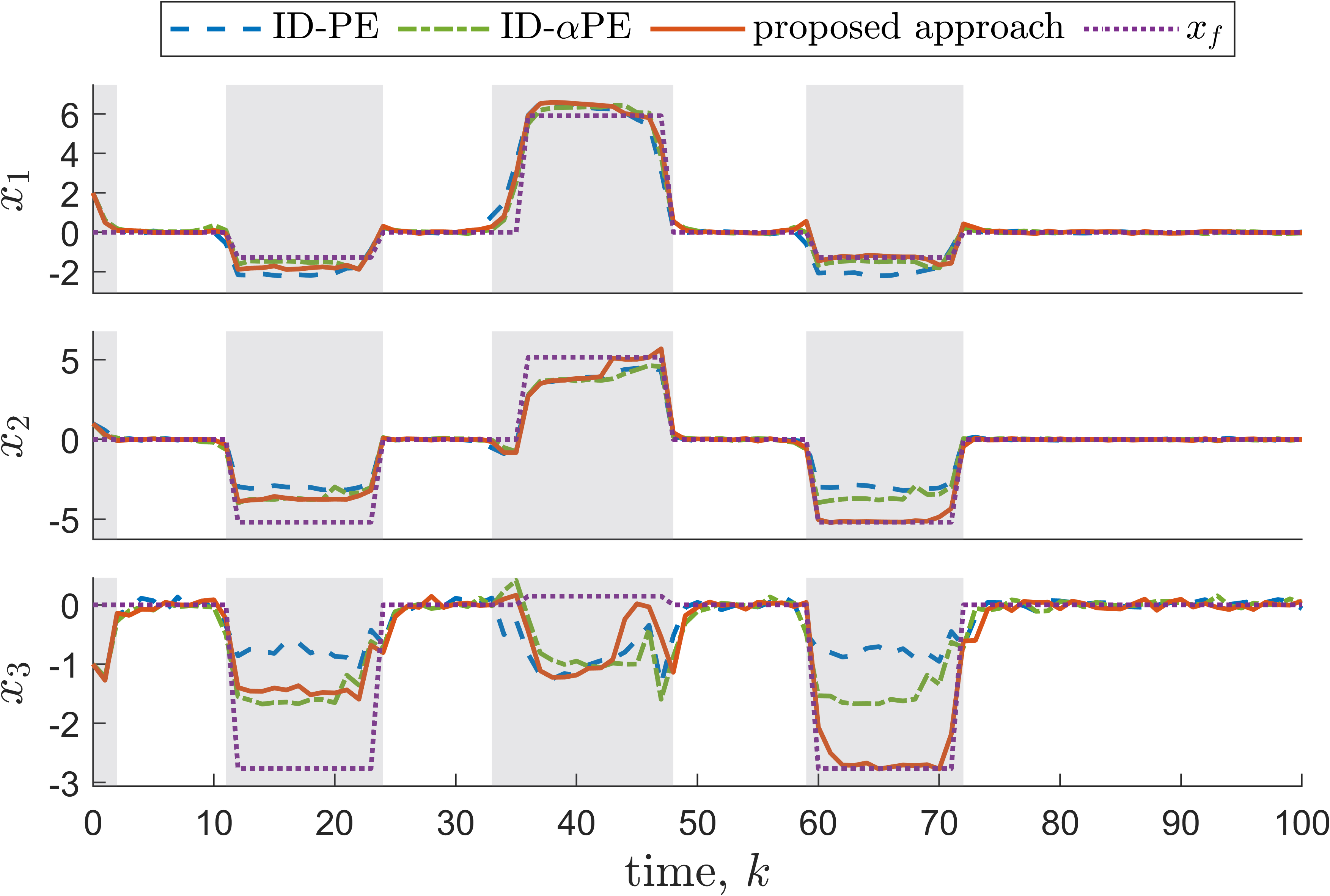
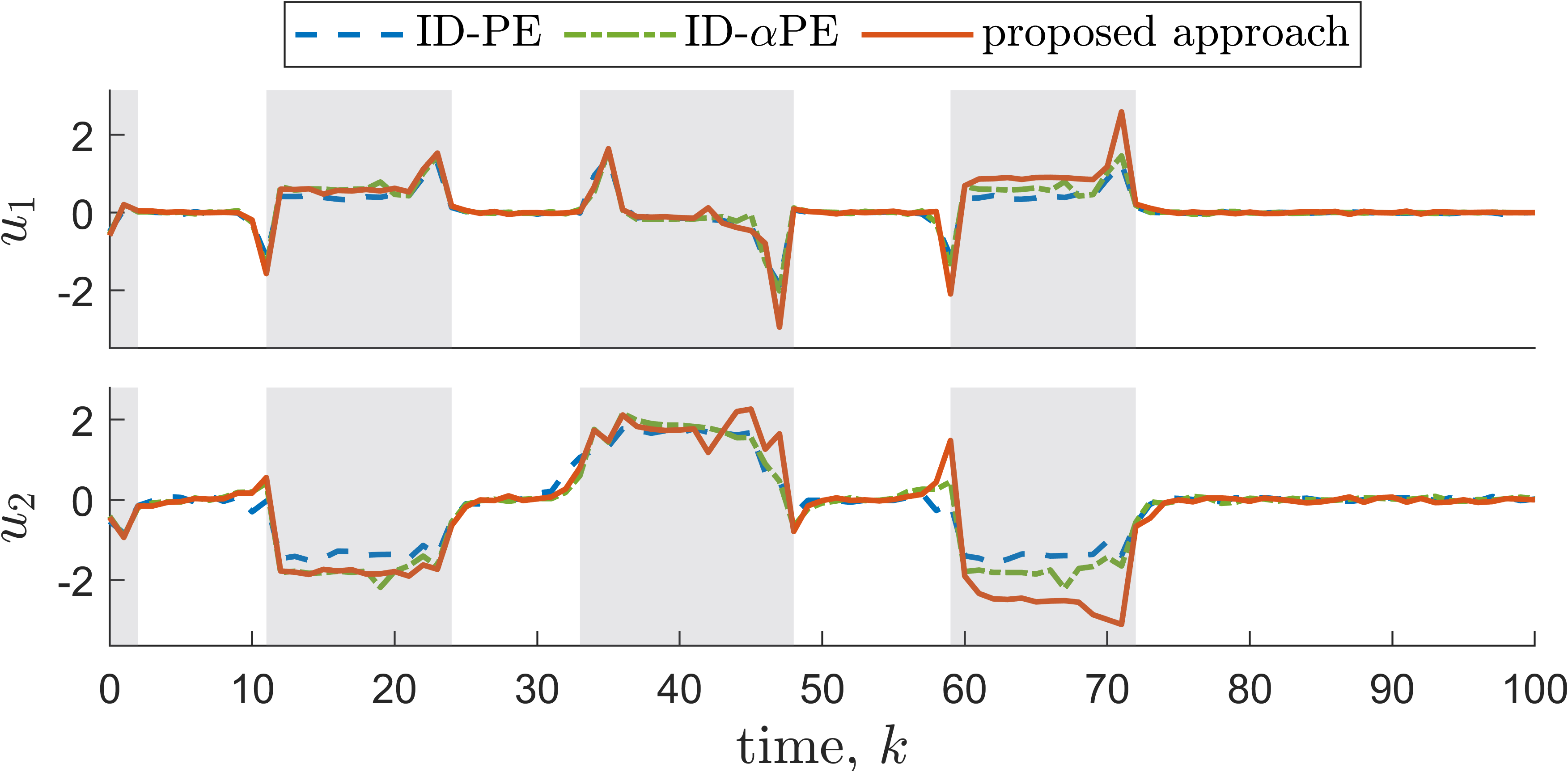
Figure 5: Closed-loop state trajectories of different controllers and the tracking reference.

Figure 6: Closed-loop input sequence of different controllers.

It can be observed that ATDPC provides a less conservative input sequence which accelerates the convergence of the system and enables a better tracking performance. It is also important to note that although ATDPC cannot tracking $x_{f}$ when $k\in[13,24]$, it successfully tracks the same reference $x_{f}$ when $k\in[61,72]$. This is attributed to the ability of the proposed active learning approach to learn form the closed-loop data. To further analyze the control performance of both methods, we introduce the performance index as follows $J_{t}\!=\!\sum_{k=0}^{100}(x(k)\!-\!x_{f}(k))^{\top}Q(x(k)\!-\!x_{f}(k))+u(k)^{\top}Ru(k)$. The performance index for each approach is represented in Table 1, which also implies the improved control performance of ATDPC.

Table 1: Comparison of the tracking costs.

	ID-PE	ID-$\alpha$PE	proposed approach
$J_{t}$	$108.7651$	$98.4251$	$68.5161$

7 Conclusion

In this work, we have investigated efficient data acquisition strategies that generate informative datasets for linear systems with bounded disturbance. The essence of the proposed approach has been to minimize the volume of the admissible systems set determined by the dataset. In the proposed active learning approach, an active input design strategy is first proposed for data acquisition in open-loop scenarios. To analyze the informativeness of the dataset, the volume of the admissible systems set is introduced as the design criterion. An overapproximation method is proposed by the inclusion relationship of ellipsoids, based on which the informativeness of the dataset is proved to be measurable with historical data and the input sequence. In the closed-loop stage, a closed-loop active learning strategy is proposed. The efficiency of this learning strategy is proved by showing that the unselected data samples are nonbenificial to the process of learning for a smaller set of admissible systems. We have followed up by applying our data acquisition strategy to adaptive tube-based data-driven predictive control. In particular, by incorporating the learned admissible systems set with the proposed dynamic nominal system, the resulting predictive control scheme is proved to be stable.

Future research could include active learning strategies for systems with stochastic disturbances. Incorporating active learning with multi-source fusion for distributed learning and control also presents an interesting direction for future work. Another intriguing question is how to design a controller that can stabilize an admissible system set that could be as large as possible, which is a dual problem to the one considered in our work. Analyzing such a problem may lead to a solution to the data-driven robust control problem, which is another potential future research topic.

Acknowlebluement

The authors would like to thank the Associate Editor and the anonymous reviewers for their suggestions which have improved the quality of the work.

[]Shilun Feng was born in Luoyang, Henan, China. He received the B.Eng. degree in automation from the Beijing Institute of Technology, Beijing, China, in 2022.

He is currently pursuing M.Sc. degree in control science and technology in the School of Automation, Beijing Institute of Technology. His research interests include event-triggered learning, data-driven control, and predictive control. []Dawei Shi received the B.Eng. degree in electrical engineering and its automation from the Beijing Institute of Technology, Beijing, China, in 2008, the Ph.D. degree in control systems from the University of Alberta, Edmonton, AB, Canada, in 2014. In December 2014, he was appointed as an Associate Professor at the School of Automation, Beijing Institute of Technology. From February 2017 to July 2018, he was with the Harvard John A. Paulson School of Engineering and Applied Sciences, Harvard University, as a Postdoctoral Fellow in bioengineering. Since July 2018, he has been with the School of Automation, Beijing Institute of Technology, where he is a professor.

His research focuses on the analysis and synthesis of complex sampled-data control systems with applications to biomedical engineering, robotics, and motion systems. He serves as an Associate Editor/Technical Editor for IEEE Transactions on Industrial Electronics, IEEE/ASME Transactions on Mechatronics, IEEE Control Systems Letters, and IET Control Theory and Applications. He is a member of the Early Career Advisory Board of Control Engineering Practice. He was a Guest Editor for European Journal of Control. He served as an associate editor for IFAC World Congress and is a member of the IEEE Control Systems Society Conference Editorial Board. He is a Senior Member of the IEEE.

[]Yang Shi received the Ph.D. degree in electrical and computer engineering from the University of Alberta, Edmonton, AB, Canada, in 2005. From 2005 to 2009, he was an Assistant Professor and an Associate Professor in the Department of Mechanical Engineering, University of Saskatchewan, Saskatoon, SK, Canada. In 2009, he joined the University of Victoria, Victoria, BC, Canada, where he is currently a Professor in the Department of Mechanical Engineering. His current research interests include networked and distributed systems, model predictive control (MPC), cyber-physical systems (CPS), robotics and mechatronics, navigation and control of autonomous systems (AUV and UAV), and energy system applications.

Dr. Shi received the University of Saskatchewan Student Union Teaching Excellence Award in 2007, and the Faculty of Engineering Teaching Excellence Award in 2012 at the University of Victoria (UVic). He is the recipient of the JSPS Invitation Fellowship (short-term) in 2013, the UVic Craigdarroch Silver Medal for Excellence in Research in 2015, the 2016 IEEE Transactions on Fuzzy Systems Outstanding Paper Award, the Humboldt Research Fellowship for Experienced Researchers in 2018. He is Vice-President on Conference Activities of IEEE IES, and Chair of IES Technical Committee of Industrial Cyber-Physical Systems. Currently, he is Co-Editor-in-Chief for IEEE Transactions on Industrial Electronics; he also serves as Associate Editor for Automatica, IEEE Transactions on Automatic Control, IEEE Transactions on Cybernetics, etc. He is General Chair of the 2019 International Symposium on Industrial Electronics (ISIE) and the 2021 International Conference on Industrial Cyber-Physical Systems (ICPS). He is a Fellow of IEEE, ASME, Canadian Academy of Engineering, Engineering Institute of Canada (EIC), and Canadian Society for Mechanical Engineering (CSME), and a registered Professional Engineer in British Columbia, Canada. []Kaikai Zheng was born in Xianyang, Shaanxi Province, China. He received the B.Eng. degree in automation from Beijing Institute of Technology, Beijing, China, in 2020. He is taking successive postgraduate and doctoral programs at the School of Automation, Beijing Institute of Technology. His research interests include event-based state estimation, system identification, event-triggered learning, and model predictive control.

References

• [1] Z.-S. Hou and Z. Wang, “From model-based control to data-driven control: Survey, classification and perspective,” Inf. Sci., vol. 235, pp. 3–35, Jan. 2013.
• [2] C. De Persis and P. Tesi, “Formulas for data-driven control: Stabilization, optimality, and robustness,” IEEE Trans. Autom. Control, vol. 65, no. 3, pp. 909–924, Mar. 2020.
• [3] G. Baggio, D. S. Bassett, and F. Pasqualetti, “Data-driven control of complex networks,” Nat. Commun., vol. 12, Mar. 2021, Art. no. 1429.
• [4] J. Luo, Y. Chen, M. Wu, and Y. Yang, “A survey of routing protocols for underwater wireless sensor networks,” IEEE Commun. Surveys Tuts., vol. 23, no. 1, pp. 137–160, 2021.
• [5] F. Davoli, C. Kourogiorgas, M. Marchese, A. Panagopoulos, and F. Patrone, “Small satellites and cubesats: Survey of structures, architectures, and protocols,” Int. J. Satell. Commun. Netw., vol. 37, no. 4, pp. 343–359, 2019.
• [6] K. Lang, “Newsweeder: Learning to filter netnews,” in Proc. Int. Conf. Mach. Learn., 1995, pp. 331–339.
• [7] B. Settles, “Active learning literature survey,” Dept. Comput. Sci., Univ. Wisconsin-Madison, Madison, WI, USA, Tech. Rep. 1648, Mar. 2009.
• [8] D. D. Lewis and W. A. Gale, “A sequential algorithm for training text classifiers,” in Proc. Int. ACM-SIGIR Conf. Res. Dev. Inf. Retr., Dublin, Ireland, 1994, pp. 3–12.
• [9] A. Raj and F. Bach, “Convergence of uncertainty sampling for active learning,” in Proc. Int. Conf. Mach. Learn., vol. 162, 2022, pp. 18 310–18 331.
• [10] H. T. Nguyen and A. Smeulders, “Active learning using pre-clustering,” in Proc. Int. Conf. Mach. Learn., 2004, p. 79.
• [11] K. Yu, J. Bi, and V. Tresp, “Active learning via transductive experimental design,” in Proc. Int. Conf. Mach. Learn., 2006, pp. 1081–1088.
• [12] L. Pronzato, “Optimal experimental design and some related control problems,” Automatica, vol. 44, no. 2, pp. 303–325, Feb. 2008.
• [13] I. Abraham and T. D. Murphey, “Active learning of dynamics for data-driven control using Koopman operators,” IEEE Trans. Robot., vol. 35, no. 5, pp. 1071–1083, Oct. 2019.
• [14] H. J. van Waarde, “Beyond persistent excitation: Online experiment design for data-driven modeling and control,” IEEE Control Syst. Lett., vol. 6, pp. 319–324, Apr. 2022.
• [15] M. Rotulo, C. De Persis, and P. Tesi, “Online learning of data-driven controllers for unknown switched linear systems,” Automatica, vol. 145, Nov. 2022, Art. no. 110519.
• [16] M. Alsalti, V. G. Lopez, and M. A. Müller, “On the design of persistently exciting inputs for data-driven control of linear and nonlinear systems,” IEEE Control Syst. Lett., vol. 7, 2023.
• [17] A. Wagenmaker and K. Jamieson, “Active learning for identification of linear dynamical systems,” in Proc. Conf. Learn. Theory, 2020, pp. 3487–3582.
• [18] A. T. Taylor, T. A. Berrueta, and T. D. Murphey, “Active learning in robotics: A review of control principles,” Mechatronics, vol. 77, Aug. 2021, Art. no. 102576.
• [19] W. Heemels, K. Johansson, and P. Tabuada, “An introduction to event-triggered and self-triggered control,” in Proc. IEEE Conf. Decis. Control, 2012, pp. 3270–3285.
• [20] C. Peng and F. Li, “A survey on recent advances in event-triggered communication and control,” Inf. Sci., vol. 457, pp. 113–125, Aug. 2018.
• [21] D. Shi, T. Chen, and L. Shi, “Event-triggered maximum likelihood state estimation,” Automatica, vol. 50, no. 1, pp. 247–254, Jan. 2014.
• [22] ——, “On set-valued kalman filtering and its application to event-based state estimation,” IEEE Trans. Autom. Control, vol. 60, no. 5, pp. 1275–1290, May. 2015.
• [23] J. Umlauft and S. Hirche, “Feedback linearization based on Gaussian processes with event-triggered online learning,” IEEE Trans. Autom. Control, vol. 65, no. 10, pp. 4154–4169, Oct. 2020.
• [24] J. Guo and J.-D. Diao, “Prediction-based event-triggered identification of quantized input FIR systems with quantized output observations,” Sci. China-Inf. Sci., vol. 63, pp. 1–12, Dec. 2020.
• [25] F. Solowjow, D. Baumann, J. Garcke, and S. Trimpe, “Event-triggered learning for resource-efficient networked control,” in Proc. Am. Control Conf., 2018, pp. 6506–6512.
• [26] F. Solowjow and S. Trimpe, “Event-triggered learning,” Automatica, vol. 117, Apr. 2020, Art. no. 109009.
• [27] J. Umlauft, T. Beckers, A. Capone, A. Lederer, and S. Hirche, “Smart forgetting for safe online learning with Gaussian processes,” in Proc. Conf. Learn. Dyn. Control, 2020, pp. 160–169.
• [28] A. Lederer, A. J. O. Conejo, K. A. Maier, W. Xiao, J. Umlauft, and S. Hirche, “Gaussian process-based real-time learning for safety critical applications,” in Proc. Int. Conf. Mach. Learn., 2021, pp. 6055–6064.
• [29] J. Jiao, A. Capone, and S. Hirche, “Backstepping tracking control using Gaussian processes with event-triggered online learning,” IEEE Control Syst. Lett., vol. 6, pp. 3176–3181, Jun. 2022.
• [30] K. He, Y. Deng, G. Wang, X. Sun, Y. Sun, and Z. Chen, “Learning-based trajectory tracking and balance control for bicycle robots with a pendulum: A Gaussian process approach,” IEEE-ASME Trans. Mechatron., vol. 27, no. 2, pp. 634–644, Jan. 2022.
• [31] J. Beuchert, F. Solowjow, J. Raisch, S. Trimpe, and T. Seel, “Hierarchical event-triggered learning for cyclically excited systems with application to wireless sensor networks,” IEEE Control Syst. Lett., vol. 4, no. 1, pp. 103–108, Jun. 2020.
• [32] Y. Zheng, S. Li, R. Wan, and Y. Wang, “Economic Lyapunov-based model predictive control with event-triggered parametric identification,” Int. J. Robust Nonlinear Control, vol. 32, no. 1, pp. 205–226, Oct. 2022.
• [33] K. Zheng, D. Shi, Y. Shi, and J. Wang, “Nonparameteric event-triggered learning with applications to adaptive model predictive control,” IEEE Trans. Autom. Control, vol. 68, no. 6, pp. 3469–3484, Jun. 2023.
• [34] J.-D. Diao, J. Guo, and C.-Y. Sun, “Event-triggered identification of FIR systems with binary-valued output observations,” Automatica, vol. 98, pp. 95–102, Dec. 2018.
• [35] K. Gatsis, “Adaptive scheduling for machine learning tasks over networks,” in Proc. Am. Control Conf., 2021, pp. 1224–1229.
• [36] ——, “Federated reinforcement learning at the edge: Exploring the learning-communication tradeoff,” in Proc. Eur. Control Conf., 2022, pp. 1890–1895.
• [37] S. J. Qin and T. A. Badgwell, “A survey of industrial model predictive control technology,” Control Eng. Practice, vol. 11, no. 7, pp. 733–764, Jul. 2003.
• [38] D. Mayne and H. Michalska, “Adaptive receding horizon control for constrained nonlinear systems,” in Proc. IEEE Conf. Decis. Control, 1993, pp. 1286–1291.
• [39] H. Fukushima, T.-H. Kim, and T. Sugie, “Adaptive model predictive control for a class of constrained linear systems based on the comparison model,” Automatica, vol. 43, no. 2, pp. 301–308, Feb. 2007.
• [40] B. A. H. Vicente and P. A. Trodden, “Stabilizing predictive control with persistence of excitation for constrained linear systems,” Syst. Control Lett., vol. 126, pp. 58–66, Apr. 2019.
• [41] V. Adetola and M. Guay, “Robust adaptive MPC for constrained uncertain nonlinear systems,” Int. J. Adaptive Control Signal Process., vol. 25, no. 2, pp. 155–167, Aug. 2011.
• [42] X. Lu and M. Cannon, “Robust adaptive tube model predictive control,” in Proc. Am. Control Conf., 2019, pp. 3695–3701.
• [43] M. Lorenzen, M. Cannon, and F. Allgöwer, “Robust MPC with recursive model update,” Automatica, vol. 103, pp. 461–471, May. 2019.
• [44] K. Zhang and Y. Shi, “Adaptive model predictive control for a class of constrained linear systems with parametric uncertainties,” Automatica, vol. 117, Jul. 2020, Art. no. 108974.
• [45] J. C. Willems, P. Rapisarda, I. Markovsky, and B. L. M. De Moor, “A note on persistency of excitation,” Syst. Control Lett., vol. 54, no. 4, pp. 325–329, Apr. 2005.
• [46] A. Mehrnoosh and M. Haeri, “An event-triggered robust data-driven predictive control with transient response improvement,” in Int. Conf. Electr. Eng., May 2023, pp. 488–491.
• [47] W. Liu, Y. Li, J. Sun, G. Wang, and J. Chen, “Data-driven self-triggering mechanism for state feedback control,” IEEE Control Syst. Lett., vol. 7, pp. 1975–1980, 2023.
• [48] W. Liu, J. Sun, G. Wang, F. Bullo, and J. Chen, “Data-driven resilient predictive control under denial-of-service,” IEEE Trans. Autom. Control, vol. 68, no. 8, pp. 4722–4737, Aug. 2023.
• [49] L. Schmitt, J. Beerwerth, M. Bahr, and D. Abel, “Data-driven predictive control with online adaption: Application to a fuel cell system,” IEEE Trans. Control Syst. Technol., vol. 32, no. 1, pp. 61–72, Jan. 2024.
• [50] S. Baros, C.-Y. Chang, G. E. Colón-Reyes, and A. Bernstein, “Online data-enabled predictive control,” Automatica, vol. 138, p. 109926, Apr. 2022.
• [51] A. Russo and A. Proutiere, “Tube-based zonotopic data-driven predictive control,” in Am. Control Conf., May 2023, pp. 3845–3851.
• [52] A. Alanwar, Y. Stürz, and K. H. Johansson, “Robust data-driven predictive control using reachability analysis,” European Journal of Control, vol. 68, p. 100666, Nov. 2022.
• [53] A. Bisoffi, C. De Persis, and P. Tesi, “Trade-offs in learning controllers from noisy data,” Syst. Control Lett., vol. 154, Aug. 2021, Art. no. 104985.
• [54] S. Boyd, L. El Ghaoui, E. Feron, and V. Balakrishnan, Linear matrix inequalities in system and control theory.   Philadelphia, PA, USA: SIAM, 1994.
• [55] H. J. van Waarde, M. K. Camlibel, and M. Mesbahi, “From noisy data to feedback controllers: Nonconservative design via a matrix S-lemma,” IEEE Trans. Autom. Control, vol. 67, pp. 162–175, Jan 2022.
• [56] I. Markovsky and F. Dörfler, “Behavioral systems theory in data-driven analysis, signal processing, and control,” Annu. Rev. Control, vol. 52, pp. 42–64, Jan. 2021.
• [57] G. H. Golub and C. F. Van Loan, Matrix computations.   Baltimore, MD, USA: JHU Press, 2013.
• [58] J. Ding and A. Zhou, “Eigenvalues of rank-one updated matrices with some applications,” Appl. Math. Lett, vol. 20, pp. 1223–1226, Dec. 2007.
• [59] F. Zhang, The Schur complement and its applications.   New York, NY, USA: Springer, 2006.
• [60] T. Hu and F. Blanchini, “Non-conservative matrix inequality conditions for stability/stabilizability of linear differential inclusions,” Automatica, vol. 46, no. 1, pp. 190–196, Jan. 2010.
• [61] M. Grant and S. Boyd. (2014, Mar.) CVX: Matlab software for disciplined convex programming, version 2.1. [Online]. Available: https://cvxr.com/cvx
{IEEEbiography}