GraphGI:A GNN Explanation Method using Game Interaction

Abstract

Graph Neural Networks (GNNs) have garnered significant attention and have been extensively utilized across various domains. However, similar to other deep learning models, GNNs are often viewed as black-box models, making it challenging to interpret their prediction mechanisms. Current graph explanation techniques focus on identifying key nodes or edges, attributing the critical data features that drive model predictions. Nevertheless, these features do not independently influence the model’s outcomes; rather, they interact with one another to collectively affect predictions. In this work, we propose a novel explanatory method GraphGI, which identifies the coalition with the highest interaction strength and presents it as an explanatory subgraph. Given a trained model and an input graph, our method explains predictions by gradually incorporating significant edges into the selected subgraph. We utilize game-theoretic interaction values to assess the interaction strength after edge additions, ensuring that the newly added edges confer maximum interaction strength to the explanatory subgraph. To enhance computational efficiency, we adopt effective approximation techniques for calculating Shapley values and game-theoretic interaction values. Empirical evaluations demonstrate that our method achieves superior fidelity and sparsity, maintaining the interpretability of the results at a comprehensible level.

1 Introduction

With the rapid growth of big data and artificial intelligence technologies, graph data has gradually evolved into a powerful data representation. Graph neural networks (GNNs) have been widely used in many fields by integrating graph data with deep neural networks, and have shown great potential in various graph-related tasks. However, like other deep learning models, GNNs are considered to be a “black box" model, where the predictions of the model cannot be interpreted from the input data. This leads to a situation where the user trusts these models completely in real-world applications. Therefore, attributing model predictions to input data is important for the progress of graph deep learning.

In recent years, a multitude of Graph Neural Network (GNN) explanation algorithms have been proposed, which can generally be categorized into two types: instance-level and model-level approaches [1]. Instance-level methods provide explanations for specific instances, whereas model-level methods offer high-level insights and a general understanding of how the deep graph model operates. Instance-level explanation methods typically utilize gradients or perturbations to obtain explanations[2, 3, 4, 5, 6, 7]. However, most of these methods assume that data features are independent of each other[8], thereby neglecting the dependencies and interactions between them. Model-level methods [9, 10], on the other hand, usually operate under the assumption that a decision can be explained using a single graph. However, this assumption [11] often fails in real-world scenarios where interactions between multiple structures are common, such as in chemical molecules where multiple structural influences may be at play.

To cope with these problems, cooperative game theory-based methods have been proposed [7, 12, 13, 14, 15]. These methods treat data features as “players" in a game, where each player’s impact on model decisions is measured by calculating the marginal contribution of player coalitions. The most notable calculation method is the Shapley value [16], which satisfies four key properties and is widely used in machine learning and deep learning for feature importance computation. Although Shapley value-based methods provide valuable insights, they present three significant limitations. Firstly, the computational cost is high due to the need to consider all possible combinations, making it an NP-hard problem. Sampling methods are often used to mitigate this, but they reduce accuracy. Secondly, these methods typically overlook structural relationships within GNNs. To mitigate this limitation, GstarX[15] employs H-N values to preserve topological information. Lastly, Shapley value can’t account for interactions between features. In fact, data features are interdependent and collectively influence the model’s decisions[17]. SubgraphX [7] attempt to consider these interactions by using subgraphs as the basis for explanations. However, treating different subgraphs as interacting coalitions fails to effectively capture the interactions between nodes or edges.

To address the aforementioned issues, we propose GraphGI, an explanation model that effectively utilizes graph topological information and the interactions between graph features. The purpose of GraphGI is to identify an explanation subgraph that captures the highest interaction strength, which corresponds to the most significant data features influencing the model’s predictions. Given the information aggregation mechanism of GNNs, for an $L$-hop GNN model, we search for the explanation subgraph within the $L$-hop neighborhood[18] Specifically, we start with an empty set and iteratively add edges that maximize the interaction value of the explanation subgraph. We employ the game-theoretic interaction value[17] as a metric for measuring interaction strength. Additionally, since the computation of the game-theoretic interaction value is based on Shapley values, we optimize this calculation using Monte Carlo sampling[7, 14]. Finally, we conduct extensive experiments on our proposed GraphGI model. The experimental results demonstrate that our model provides superior explanations compared to other models, exhibiting better fidelity and sparsity.

The main contributions of the paper are as follows:

• We propose GraphGI, an explanatory framework for graph neural networks based on game interaction theory, and validate its effectiveness through experiments.

• GraphGI elevates the interaction explanation of graph data structures from the subgraph level to the edge-to-edge interaction level.

• We introduce an efficient computational method for game interactions, significantly improving computational efficiency.

2 Related Work

Explanatory models for GNNs can be divided into two types: instance-level and model-level, in our work we concentrate on instance-level explanation. The current instance-level explanations can be classified into gradients/features-based method, decomposition method, surrogate method, perturbation method. Additionally, Shapley-based methods have gained widespread attention; these methods generate explanations by using the Shapley value as a metric to assess the importance of data features. The purpose of these methods is to find the nodes or links in the input data that play a key role in the model’s predicted results, while ignoring the interactions between these data structures. These methods are described below:

• Gradient/feature-based method: These methods employ gradient or hidden feature mapping values as an approximation of input saliency. Representative methods are Saliency[2], Guided Backpropagation[2], CAM[5] and GradCAM[5]. The main difference between these methods is the process of gradient backpropagation and the way different hidden feature mappings are combined. However, these methods also have significant drawbacks, due to the topological and non-linear nature of the graph data, this method does not produce accurate interpretations and it is difficult to capture the interactions between the graph data in this method.

• Decomposition method: These methods decomposes the predictions of the original model into a number of terms to measure the importance of the input features. These terms are considered as importance scores for the corresponding input features. This type of method directly examines the model parameters to reveal the relationship between the features in the input space and the predictions in the output space. Representative methods in this category are LRP[3], Excitation BP[19] and GNN-LRP[20]. This approach requires knowledge of the model parameters and is therefore not applicable to the interpretation of black-box models. Furthermore, decomposition methods do not capture the interactions between data structures.

• Surrogate methods: This class of methods revolves around the fundamental concept of employing simple and interpretable surrogate models to approximate the predictions of neighboring regions in the input data made by complex deep models. Representative methods in this category include PGM-Explainer[8], Graph-Lime[21] and RelEx[22]. However, it is important to note that surrogate methods often necessitate additional computational resources for training the surrogate model. Additionally, these methods do not have the capability to predict local data structures, which limits their ability to accurately compute interactions between different graph data structures.

• Perturbation methods: These methods involve the removal or addition of specific information such as nodes, edges, or features in the original graph. The modified graph is then fed back into the model for prediction, providing insights into the significance of the perturbed information. Representative methods in this category include PGExplainer[4], GNNExplainer[6], GraphSVX[13], EdgeSHAPer[14], GstarX[15], Zorro[23], FlowX[24] and GraphMask[25]. However, it is important to acknowledge that perturbation methods are susceptible to noise and outliers, and determining the appropriate magnitude of perturbation can be challenging. Additionally, most of these methods assume linear independence among features, thus neglecting the interactions between different data structures.

• Shapley-based Methods: In the context of GNNs, Shapley value-based methods can be categorized into two types based on the challenges they address: computational efficiency and graph structural considerations. The first category includes methods such as SubgraphX[7], GNNShap[12], GraphSVX[13] and EdgeSHAPER[14]. which aim to enhance the computational efficiency of Shapley value through various sampling techniques, thereby identifying high-scoring edges or nodes as explanations. The second category features methods like GstarX[15], which recognize that the Shapley value does not account for the connectivity structures of different coalitions. Consequently, GstarX opts for a structure-aware value from cooperative game theory to provide explanations. Overall, existing Shapley-based methods primarily focus on making the Shapley value more applicable to GNNs efficiently, without delving deeply into the interactions among graph data features.

Broadly speaking, as noted in previous work[8], most of the aforementioned approaches assume that features are independently associated, thereby neglecting their dependencies and interactions. Notably, recent methods such as SubgraphX have advanced GNN explanations from the level of nodes, edges, or node features to the level of subgraphs. However, treating different subgraphs as interacting coalitions fails to effectively capture the interactions between nodes or edges. In contrast, our GraphGI employs game-theoretic interaction values as an evaluation metric and treats explanations as a sequential decision-making process. This approach incrementally considers the interactions among different coalitions, leading to more faithful and rational explanations.

3 Problem Definition and Preliminaries

Notations. Let ${G=(V,E)}$ denote an undirected and unweighted graph, where ${V}=\{{{v}_{1}},\cdots,{{v}_{N}}\}$ denotes the set of nodes and ${E}=\{{{e}_{1}},\cdots,{{e}_{M}}\}$ denotes the set of edges. The adjacency matrix of graph ${G}$ is denoted as ${{A}}\in{\{0,1\}^{N\times N}}$, where ${{{A}}_{ij}}=1$ if nodes $i$ and $j$ are connected and ${{{A}}_{ij}}=0$ otherwise.Additionally, ${{X}}\in{{C}}^{N\times N}$ denote the node feature martrix.We consider node classification task is mapped to one of ${C}$ classes. If $f$ is a GNN model, the predicted class of a node can be expressed as $\hat{y}=f({{A}},{{X}},{{v}})$.

Graph Neural Networks. GNNs (Graph Neural Networks) are a powerful class of neural networks that can effectively model and analyze complex relationships and dependencies within graph-structured data. They utilize a message-passing scheme to propagate information between nodes, enabling them to capture both local and global graph information. The core computation of GNNs can be described by the following equation:

$$h_{v}^{(l+1)}=\sigma\left(\sum_{u\in\mathcal{V}(v)}\frac{1}{c_{u,v}}W^{(l)}h_{u}^{(l)}\right)$$ (1)

where $h_{v}^{(l)}$ represents the hidden representation of node $v$ at layer $l$, $\mathcal{V}(v)$ denotes the set of neighbors of node $v$, $W^{(l)}$ is the weight matrix at layer $l$, $\sigma(\cdot)$ is the activation function, and $c_{u,v}$ is a normalization factor. Equation 1 captures the iterative process of message passing and aggregation, allowing GNNs to capture and integrate information from the neighborhood of each node, producing informative and context-aware node representations.

3.1 GNN Explanations

The purpose of explanation methods for GNNs is to identify significant data features that underpin model reasoning and predictions. Given an original graph $G(V,E)$ and a pre-trained model $f$ that needs to predict $\hat{y}$ for a node $v$, GNN explainers aim to extract an essential subgraph $G_{s}(V_{s},E_{s})$ from the original graph as an explanation for the model’s predictions.In particular, the explanation problem involves determining how to measure the importance of nodes or edges in the original graph $G(V,E)$ and how to obtain an important subgraph $G_{s}(V_{s},E_{s})$.Therefore, the explanation methods for graph neural networks can be formalized as:

$$G_{s}(V_{s},E_{s})=\text{Exp}(G(V,E))$$ (2)

where $\text{Exp}(\cdot)$ denotes a GNN explainer. In this work, we focus on explanations of node classifications.

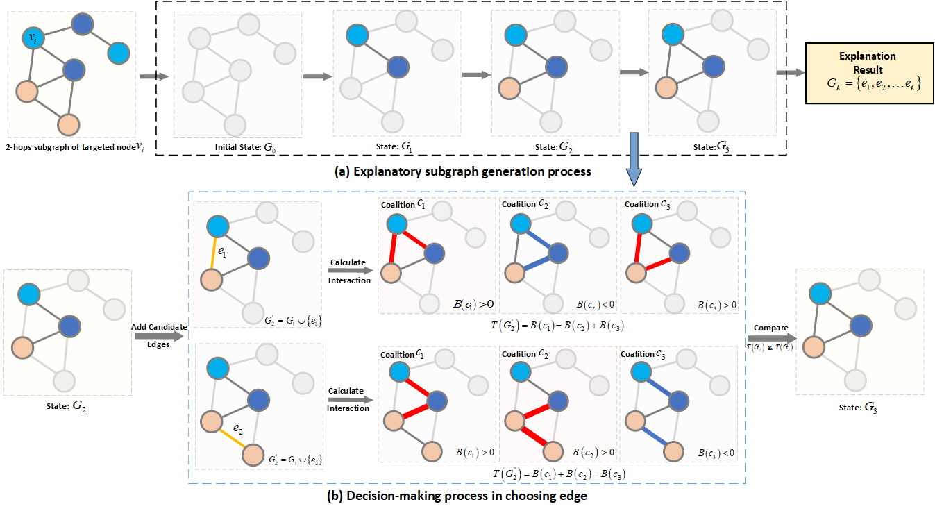
Figure 1: Illustration of the proposed GraphGI framework (a) Explanatory subgraph generation process; (b) Decision-Making Process: Transition from State 3 to State 4. The red edges represent positive interaction alliances, while the blue edges represent negative interactions.

3.2 Shapley Value

The Shapley value [16] is a method from Game Theory. It describes how to fairly distribute the total gains of a game to the players depending on their respective contribution, assuming they all collaborate. It is obtained by computing the average marginal contribution of each player when added to any possible coalition of players. This method is widely applied in explaining machine learning [26, 27] and deep learning model[7, 13]. The contribution of player $i$ can be formalized as follows:

$$\varphi_{v}(i|N)=\frac{1}{n!}\sum_{S\subseteq N\setminus{i}}\frac{(n-|S|-1)!|S|!}{n!}[v(S\cup{i})-v(S)]$$ (3)

where $N$ represents the set of all players, $v$ is the game function mapping subsets to real numbers, $S$ is a subset, $\varphi_{v}(i|N)$ is the Shapley value of player $i$, $|S|$ denotes the number of players in $S$, $n$ represents the total number of players, and $v(\emptyset)=0$. In graph neural networks, nodes, edges, and features are assumed to be “players" for explaining the model.

3.3 Game-theoretic Interaction

In the rich domain of cooperative game theory, interactions among players are crucial for understanding their strategic choices and behavioral patterns. [28] introduced a method to quantify player interactions based on the Shapley value, referred to as Game-theoretic Interaction. This value provides a mathematically rigorous representation of the interactions among players, grounded in the axioms of linearity, dummy players, and symmetry. Specifically, for any set of players $S\subseteq N$, they can be treated as a single player denoted as $[S]$, the game-theoretic interaction value $I([S])$ is calculated as follows:

$$I_{v}(S)=\varphi_{v}([S]|N[S])-\sum_{i\in S}\varphi(i|N_{i})$$ (4)

where, $\varphi v[S]|N[S]$ represents the Shapley value of the coalition $[S]$. We compute the Shapley value over the player set $N[S]=N\setminus S\cup{[S]}$. Similarly, $\varphi(i|N_{i})$ denotes the Shapley value of player $i$ which in coalition $S$.

The sign of the game-theoretic interaction value directly influences players’ cooperative decisions. A positive value typically indicates that cooperation among players can generate additional value, meaning that the total benefit of cooperation exceeds the sum of their individual actions. Conversely, a negative value suggests that cooperation may lead to a loss in value. To better assess the interactions among players, interaction strength[17] is defined based on the game-theoretic interaction value to reflect both positive and negative interactions among multiple players. Assuming $I_{+}(S)$ represents all positive interactions within coalition $S$, and $I_{-}(S)$ represents negative interactions, the interaction strength $T(S)$ is calculated as follows:

$$T(S)=I_{+}(S)-I_{-}(S)$$ (5)

4 The Proposed Method

This section presents the proposed GNN explanation method, GraphGI. Fig.1 illustrates the process of progressively generating the explanation subgraph and the decision-making process for selecting candidate edges. Our model is designed for the task of graph node classification. Fig.1(a) illustrates the process of subgraph search. Starting from an empty set and initiating from the target node $v_{i}$, we progressively search for and add edges to the set that maximize subgraph interactions, ultimately generating the explanatory subgraph. Fig.1(b) shows the decision-making process for each selection. By adding candidate edges to the selected subgraph, we calculate the positive and negative interactions of the new subgraph. By comparing the interaction strengths between subgraphs, we select the edge that maximizes the new subgraph interaction value to be added to the set.

4.1 Game-Interactions Scoring Function

In our proposed GraphGI, the choice of significant edges is highly depending on the scoring function. It is crucial for measuring the importance of different subgraphs. In the past, one conventional method is to remove edges from a subgraph, then feed both the modified subgraph and the original subgraph into a pre-trained model $f(\cdot)$. The importance of edges can be assessed by comparing the output probabilities of the model. However, it cannot capture the interactions between different edges, thus affecting the explanation results. Additionally, another widely used evaluation method is the Shapley value. The Shapley value is an index used in game theory to measure the cooperative properties of a game by assessing the contribution of each player to the game’s gain. When applied it to Graph Neural Networks (GNNs), the predictions of the GNN are usually considered as the payoff of a game, with various graph structures acting as the players. Formally, the Shapley value can be formalized as follows:

$$\varphi(e_{i}|E)=\frac{1}{n!}\sum_{E^{\prime}\subseteq E\setminus{e_{i}}}\frac{(n-|E^{\prime}|-1)!|E^{\prime}|!}{n!}[f(E^{\prime}\cup{e_{i}})-f(E^{\prime})]$$ (6)

here, $n$ is the number of all edges and $E$ is a set of all egdes, $E^{\prime}$ is a subset of $E$, $|E|$ is the size of $E^{\prime}$. $f(\cdot)$ is a pre-trained GNN model, and $f(E^{\prime}\cup{e_{i}})-f(E)$ is the marginal contribution of player $e_{i}$’s to coalition $E^{\prime}$. The Shapley value is the only method that satisfies four key properties: linearity, symmetry, dummy and efficiency these properties ensure the validity and reliability of the explanation results [28, 16, 17]. The Shapley value ranges between $[-1,1]$. If the value is positive, it indicates that the current edge has a positive impact on the model’s prediction; conversely, a negative value suggests a negative impact. The magnitude of the it represents the strength of player’s influence. However, Shapley values can only measure the contribution of individual players in cooperative games and cannot effectively reflect the interactions among players, thus it cannot adequately account for interactions between graph structures. Therefore, in this work, we adopt Game-Interaction values as the scoring function [17, 28]. The Game-Interaction values is a method based on cooperative game theory that can measure the interaction among multiple players in the game.Assume the set of edges $A\subseteq E$ is a coalition, we treat the coalition as a signal player $[A]$ which participate in game. The Game-Interaction values of coalition $[A]$ can be defined as follows:

$$B([A])=\varphi([A]|E[A])-\sum_{e_{i}\in A}\varphi(e_{i}|E_{e_{i}})$$ (7)

where $\varphi([A]|E[A])$ represents the Shapley value of the coalition $[A]$. We compute the Shapley value over the player set $E[A]=N\setminus E\cup{[A]}$. Similarly, $\varphi(e_{i}|E_{e_{i}})$ denotes the Shapley value of egde $e_{i}$ when the model prediction is played without the players in $A\setminus{e_{i}}$. In particular, due to the discrete nature of the graph data, it is difficult to directly synthesise multiple edges directly into a single edge. To preserve the structural information of the original graph, we did not directly treat the coalition $[A]$ as a single new player when calculating the game-theoretic interactions of the coalition. Therefore, in Equation 7, the expression $E[A]=N\setminus E$ differs from that in Equation 4.

In fact, the interaction value obtained from Equation 7 represents the net result of all positive and negative interactions within coalition $A$. We believe that interactions should reflect both positive and negative effects. Therefore, we employ a specialized metric to quantify the positive and negative effects within the edge set $A\subseteq E$. Our objective is to partition all edges in $A$ into multiple coalitions with varying interaction effects, denoted as $\Omega=\{C_{1},C_{2},\dots,C_{k}\}$. $\Omega$ represents a partition of set $A$. The positive interaction for $A$ can then be expressed as the sum of the positive effects of all sub-coalitions, formalized as:

$$B_{\max}([A])=\max_{\Omega}\sum_{C_{i}\in\Omega}\varphi(C_{i}|E[C_{i}])-\sum_{e_{i}\in A}\varphi(e_{i}|E_{i})$$ (8)

here $\varphi(C_{i}|E[C_{i}])$ is computed over $E[C_{i}]=E\setminus A\cup{[C_{i}]}$, and $\varphi(e_{i}|E_{i})$ is computed over $E_{e_{i}}=E\setminus A\cup{e_{i}}$. Similarly, we can use $B_{\min}([A])$ to roughly quantify the negative interaction effects in the set $A$. It can be formulated as:

$$B_{\min}([A])=\min_{\Omega}\sum_{C_{i}\in\Omega}\varphi(C_{i}|E[C_{i}])-\sum_{e_{i}\in A}\varphi(e_{i}|E_{e_{i}})$$ (9)

Therefore, we define a metric $T([A])$ to measure the importance of positive and negative interaction effects as follows:

$$T([A]) =B_{\max}([A])-B_{\min}([A])$$ (10)

$$=\max_{\Omega}\sum_{C_{i}\in\Omega}\varphi(C_{i}|E[C_{i}])-\min_{\Omega}\sum_{C_{i}\in\Omega}\varphi(C_{i}|E[C_{i}])$$

4.2 Subgraph Exploration

In our proposed GraphGI, we employ a greedy subgraph exploration strategy to generate explanation subgraphs. The basic idea is integrating the screening strategy[26] with the Game-Interaction value of subgraph, the explanation subgraph starts from an empty set and gradually selects edges that maximize the interaction value of the subgraph. Formally, the objective function is as follows:

$$e_{k}^{*}=\arg\max_{e_{k}\in\mathcal{O}_{k}}T\left(\left[G_{k}^{*}\right]\right)-T\left(\left[G_{k-1}^{*}\right]\right),\quad k=1,2,\cdots,K$$ (11)

$$G_{k}^{*}=e_{k}\mid{G}_{k-1}^{*}$$ (12)

where $G_{k-1}^{*}$ denotes the subgraph selected at step $k-1$, $G_{0}=\emptyset$ .At the k-th step.$e_{k}^{*}$ is the edge selected from the pool of edge candidates $\mathcal{O}_{k}$, $\mathcal{O}_{k}$ is the set of adjacent edges of $e_{k-1}$. $G_{k}$ is established by merging $G_{k-1}^{*}$ and $e_{k}^{*}$, and $T\left(\left[G_{k}^{*}\right]\right)$ denotes the Game-Interaction value of $G_{k}^{*}$. We repeat this process until we find the subgraph with the highest interaction value as the final explanatory subgraph.

At each step, Eq.11 guides the edge selection, which estimates the Game-Interaction of $G_{k}^{*}$, conditioning on the previously selected subgraph $G_{k-1}^{*}$. In particular, if $T\left(\left[G_{k}^{*}\right]\right)-T\left(\left[G_{k-1}^{*}\right]\right)>0$, it indicates that the addition of the edge $e_{k}$ strengthens the interaction intensity of the subgraph ${G}_{k-1}^{*}$. Therefore, it can be considered that the addition of the edge e has a positive effect on the prediction of the model $f(\cdot)$. Otherwise, a negative influence indicates that $e_{k}$ is not suitable to participate in the interpretation at step k. Hence, it ensures that the final generated explanatory subgraph has the highest interaction value and the effectiveness of the entire explanation.

A straightforward solution to optimising Eq.13 is by greedy sequential exhaustive search. One of the steps is to compute the Game-Interaction value of all candidate edges to add subgraphs, and then add the edge with the highest score, connecting the previously added edges. This step iteration is repeated K times. Greedy sequential exhaustive search is at the heart of many feature selection algorithms, having shown great success. However, this method, and the computation of game interactions based on the Shapley value computation method, require computing for all possible coalitions, which consumes a lot of computational resources. Therefore, optimizing the computation time is also an important challenge.

4.3 Efficient Computations

To improve computational efficiency, we adopted an efficient Shapley value computation method[7] and applied Monte Carlo sampling[14] to the possible coalitions in both Shapley value computation and game interaction computation.

In graph neural networks, the features of a target node are updated by gathering information from a restricted neighborhood. If there are $L$ layers of GNN in the graph model $f(\cdot)$, then only neighboring nodes within $L$ hops are considered for information aggregation. This aggregation process can be viewed as interactions between various graph structures. As a result, subgraph ${G}_{i}$ primarily interacts with neighbors within $L$ hops. However, due to the complexity of graph data, computing the Shapley value still requires calculations for a large number of coalitions, which is a crucial factor contributing to the complexity of Shapley value computation. Hence, in our work, we employ Monte-Carlo sampling to compute shapley value. Specifically, for sampling step $i$, we sample a coalition set $E^{\prime}$ from the player set $E_{i}\setminus{e_{i}}$ and compute its marginalized contribution. Then the averaged contribution score for multiple sampling steps is regarded as the approximation of $\phi(e_{i})$. Formally, it can be mathematically formulated as

$$\varphi(e_{i}|E_{i})=\frac{1}{T}\sum_{t=1}^{T}(f(E^{\prime}\cup{e_{i}})-f(E^{\prime}))$$ (13)

where $T$ is the total sampling steps. Similarly, we also employed Monte Carlo sampling in computing Game-Interactions to obtain possible coalitions. The Game-Interaction value with sampling can be denoted as:

$$B([A])=\frac{1}{M}\sum_{t=1}^{M}\sum_{C_{i}\in\Omega}\varphi(C_{i}|N[C_{i}])-\sum_{e_{i}\in A}\varphi(e_{i}|E_{i})$$ (14)

where $M$ is the total sampling steps. Eventually, we conclude the computation steps 6 our proposed GraphGI in Algorithm 1 and 2.

Algorithm 1 The algorithm GraphGI.

  Input: GNN model $f(\cdot)$ with $L$-layers, input graph ${G}$ with edges $E=\{e_{1},\dots,e_{k}\}$, target node $v_{0}$.

  Initialization: Obtain $L$-hop subgraph $G_{0}$ of the target node $v_{0}$ with edges $E_{0}=\{e_{1},\dots,e_{r}\}$, $G_{0}\subseteq G$. Initialize an empty set coalition $C,C=\emptyset$ and find an edge in the set of neighboring edges $\mathcal{O}$ of the target node $v$ that has the maximum Shapley value to add to the set $C$

  while  $\mathcal{O}=\emptyset$ or the interaction strength of $C$ is no longer increasing do

     for all possible edges $e_{i}$ of $\mathcal{O}$ do

        Add edge to $e_{i}$ the coalition $C_{pre}$ to get the current coalition $C_{now}$,$C_{now}=C_{pre}\cup e_{i}$

        Calculate the Game-Interaction values of $C_{pre}$ and $C_{now}$ with Algorithm 2.

     end for

     Select the edge $e$ with Equation11, $C=C\cup{e}$

     update($\mathcal{O}$)

  end while

  Return: A coalition $C$ of selected edges which can be treated the explanation subgraph.

Algorithm 2 The algorithm of Game-Interaction value.

  Input: GNN model $f(\cdot)$ with $L$ layers, target node $v_{0}$, coalition $E^{\prime}$ with $k$ edges $\{e_{1},\dots,e_{k}\}$, Monte-Carlo sampling steps $T$.

  Initialization: Obtain $L$-hop subgraph $G_{0}$ of the target node $v_{0}$ with edges $E_{0}=\{e_{1},\dots,e_{r}\}$. Initialize an empty set of positive interactions $S_{+}$, and an empty set of negative interactions $S_{-}$

  for $i=1$ to $T$ do

     Sampling a coalition set $E_{i}$ from $E_{s}\setminus E^{\prime}\cup\left[E^{\prime}\right]$

     Caculate the shapley value of coalition $E_{i}$ with Equation 7

     if  $\phi(\left[E_{i}]\right)>0$ then

        $S_{+}$ append $\phi\left(\left[E_{i}\right]\right)$

     else

        $S_{-}$ append $\phi\left(\left[E_{i}\right]\right)$

     end if

  end for

  Return: $T\left(\left[E^{\prime}\right]\right)=sum\left(S_{+}\right)-sum\left(S_{-}\right)$

5 Experimental Settings

5.1 Experimental Datasets

We conducted rich experiments to validate the effectiveness of our model on different datasets and GNN models. Table 1 presents the statistics and attributes of datasets. We evaluate our method on the node classification task using seven datasets, including four synthetic datasets and three real-world datasets, summarized as follows:

• BA-Shapes [6]: This graph is formed by randomly connecting a base graph to a set of motifs. The base graph is a Barabasi-Albert (BA) graph with 300 nodes. It includes 80 house-structured motifs with five nodes each, formed by a top, a middle, and a bottom node typeels are determined by the chemical functionalities of molecules.

• BA-Community[6]: The BA-community graph is a combination of two BA-Shapes graphs. The features of each node are assigned based on two Gaussian distributions. Also, nodes are assigned a class out of eight classes based on the community they belong to.

• Tree Cycle[6]: This consists of a 8-level balanced binary tree as a base graph. To this base graph, 80 cycle motifs with six nodes each are randomly connected. It just has two classes; one for the nodes in the base graph and another for nodes in the defined motif.

• Tree Grids[6]: This graph uses same base graph but a different motif set compared to the tree cycle graph. It uses 3 by 3 grid motifs instead of the cycle motifs.

• Cora[29]: The dataset, commonly used in recent graph deep learning research, consists of machine learning papers. It includes a total of 2,708 samples, each representing a scientific paper. All samples are categorized into eight distinct classes: case-based, genetic algorithms, neural networks, probabilistic methods, reinforcement learning, rule learning, and theory.

• CiteSeer[29]: In the CiteSeer dataset (citation network), the papers are categorized into six classes: Agents, AI (Artificial Intelligence), DB (Databases), IR (Information Retrieval), ML (Machine Learning), and HCI (Human-Computer Interaction). The dataset contains a total of 3,312 papers, with recorded citation information between them. After removing stop words and words that appear less than ten times in the documents, we obtained 3,703 unique words.

• PubMed[29]: The PubMed dataset (citation network) includes 19,717 scientific publications on diabetes from the PubMed database, categorized into three classes. The citation network comprises 44,338 links. Each publication in the dataset is described by a TF/IDF weighted word vector from a dictionary of 500 unique words.

Since interpretation of the target task is time-consuming, we selected only some of the nodes in the test set for our experiments.

Table 1: Comparison of various datasets

	BA-shapes	BA-community	Tree-cycle	Tree-grid	Cora	Citeseer	Pubmed
# of Edges	4110	8920	1950	3410	5489	4732	44338
# of Nodes	700	1400	871	1231	2708	3327	19717
# of Classes	4	8	2	2	6	7	3

Table 2: Model Training and Test Accuracies

Dataset	GCN		GIN
	Train	Test	Train	Test
BA-shapes	99.74	94.15	99.23	93.29
BA-community	98.15	92.73	99.11	94.48
Tree-cycle	99.98	89.86	99.96	90.31
Tree-grid	99.94	91.46	99.99	94.32

5.2 Models

We chose three GNN models to train on the above four datasets, two-layer GCN[30] and two-layer GIN[31]. we used ReLU as the activation function in training, a dropout of 0.5, and a cross-entropy function as the loss function. We train the model for 800 epochs at a learning rate of 0.01. Table 2 shows the accuracy of the training and test sets.

5.3 Evalution metrics

We employ Fidelity[6] and Sparsity[6] metrics to evaluate the performance of our model. Give a graph $G$, its prediction class $y$ and its explanatory subgraph $G_{S}$. Fidelity removes the filtered important graph structures and retains only the non-important parts, it can be computed as:

$$Fidelity=\frac{1}{N}\sum_{i=1}^{N}(f(G)_{y}-f(G\setminus G_{s})_{y})$$ (15)

where $N$ is the number of testing samples,$f(G)_{y}$ is the probability of class $y$ for original graph $G$. Specially, fidelity demonstrates the importance of explanatory subgraphs by probability. In addition, we employ Sparsity to evaluate the fraction of edges are selected in the explanations.Then it can be computed as:

$$\textit{Sparsity}=\frac{1}{N}\sum_{i=1}^{N}(1-\frac{|G_{s}|}{|G|})$$ (16)

where $|G_{i}|$ denotes the number of important edges in explanatory subgraph $G_{i}$ and $|G|$ means the number of edges in $G$. Generally speaking, good explanations should select fewer edges (high Sparsity) but lead to significant prediction drops (high Fidelity).

Table 3: Fidelity scores for the top 20 nodes in the test set for 2-hops GCN explanations. Higher values signify better performance, with bold black denoting the optimal outcome.

Method	Metric	BA-shapes	BA-community	Tree-cycles	Tree-Grid
SubgraphX	Fidelity	64.04 $\pm$ 0.26	59.96 $\pm$ 0.12	99.18 $\pm$ 0.08	87.63 $\pm$ 0.44
	Sparsity	42.38 $\pm$ 0.46	64.94 $\pm$ 0.45	15.38 $\pm$ 0.57	26.53 $\pm$ 0.42
PGExplainer	Fidelity	75.28 $\pm$ 0.73	61.23 $\pm$ 0.21	99.22 $\pm$ 0.05	87.60 $\pm$ 0.34
	Sparsity	32.38 $\pm$ 0.11	53.08 $\pm$ 0.46	55.48 $\pm$ 0.20	56.01 $\pm$ 0.62
GNNExplainer	Fidelity	46.27 $\pm$ 0.78	48.32 $\pm$ 0.42	93.86 $\pm$ 0.24	75.50 $\pm$ 0.53
	Sparsity	50.12 $\pm$ 0.17	54.11 $\pm$ 0.64	45.07 $\pm$ 0.28	54.38 $\pm$ 0.63
PGM-Explainer	Fidelity	62.71 $\pm$ 0.23	59.35 $\pm$ 0.15	95.22 $\pm$ 0.13	81.23 $\pm$ 0.61
	Sparsity	39.56 $\pm$ 0.68	42.65 $\pm$ 0.59	34.14 $\pm$ 0.24	54.84 $\pm$ 0.72
GraphGI	Fidelity	84.84 $\pm$ 0.53	61.51 $\pm$ 0.23	99.19 $\pm$ 0.29	89.10 $\pm$ 0.34
	Sparsity	85.75 $\pm$ 0.51	90.61 $\pm$ 0.32	71.37 $\pm$ 0.55	78.24 $\pm$ 0.36

Table 4: Fidelity scores for the top 20 nodes in the test set for 2-hops GIN explanations. Higher values signify better performance, with bold black denoting the optimal outcome.

Method	Metric	BA-shapes	BA-community	Tree-cycles	Tree-Grid
SubgraphX	Fidelity	74.24 $\pm$ 0.32	64.23 $\pm$ 0.24	94.18 $\pm$ 0.99	89.32 $\pm$ 0.18
	Sparsity	41.14 $\pm$ 0.51	52.42 $\pm$ 0.46	54.68 $\pm$ 0.83	38.53 $\pm$ 0.64
PGExplainer	Fidelity	81.28 $\pm$ 0.35	78.63 $\pm$ 0.92	93.22 $\pm$ 0.78	87.60 $\pm$ 0.84
	Sparsity	32.38 $\pm$ 0.11	50.28 $\pm$ 0.53	48.32 $\pm$ 0.26	53.23 $\pm$ 0.24
GNNExplainer	Fidelity	71.27 $\pm$ 0.32	63.32 $\pm$ 0.42	92.22 $\pm$ 0.18	87.50 $\pm$ 0.53
	Sparsity	56.10 $\pm$ 0.32	53.11 $\pm$ 0.13	53.74 $\pm$ 0.35	52.18 $\pm$ 0.51
PGM-Explainer	Fidelity	72.87 $\pm$ 0.27	64.89 $\pm$ 0.24	96.38 $\pm$ 0.86	87.50 $\pm$ 0.53
	Sparsity	52.10 $\pm$ 0.62	42.11 $\pm$ 0.56	45.65$\pm$ 0.24	61.38 $\pm$ 0.56
GraphGI	Fidelity	89.24 $\pm$ 1.35	86.63 $\pm$ 0.87	97.63 $\pm$ 0.63	87.63 $\pm$ 0.62
	Sparsity	89.75 $\pm$ 0.36	63.53 $\pm$ 0.26	81.46 $\pm$ 0.64	84.23 $\pm$ 1.12

5.4 Baseline

The proposed method is compared with three subgraph exploration baseline methods such as PGExplainer[4], GNNExplainer[6], SubgraphX[7] and PGM-Explainer[18]. We summarize these baseline as:

• PGExplainer: PGExplainer is an improved approach on GNNExplainer which also uses mutual information for explanation. It explain edges by training an agent neural network. We train PGExplainer for 20 epochs with a 0.05 learning rate.

• SubgraphX: SubgraphX employs Monte Carlo tree search to explore explanatory subgraph. We use a "zero-filling" approach to calculate the Shapley value, and the number of Monte Carlo samples is 100. The maximum number of nodes in the interpretation subgraph is set to 5.

• GNNExplainer: uses mutual information to learn important edges and features. Note that the PyTorch Geometric implementation of GNNExplainer uses the full graph instead of a computational graph. We use l-hop-subgraph in explanations to reduce the explanation time. We train GNNExplainerfor 200 epochs with a 0.01 learning rate for explanations.

• PGM-Explainer: learns node importance by using aprobabilistic graphical model. We use default settings for PGM-Explainer.

For our customized methods, we employed the same Shapley value calculation method as used in our proposed GraphGI. The difference lies in how the final explanation subgraph is generated. The objective of these methods is to demonstrate that game-theoretic interaction values can provide more effective model explanations.

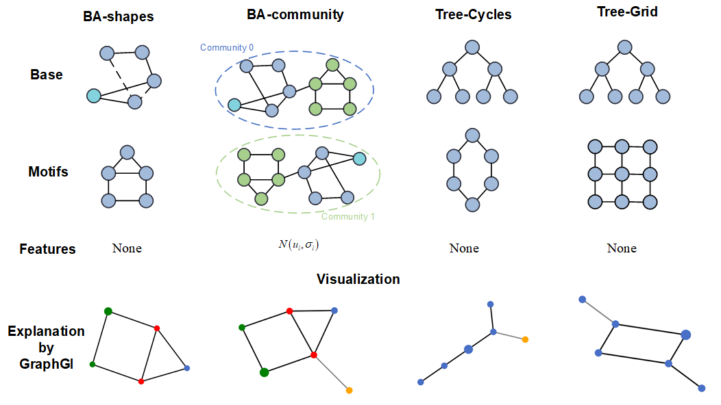
Figure 2: Illustration of the Synthetic Dataset and Visualization of GraphGI Explanation Results

5.5 Test environment

We conduct our experiments useing one NVIDA 2080Ti GPU on Intel CPU.We use Python 3.7.0, PyTorch 1.1.13 and PyTorch Geometric 2.3.1.

Table 5: Fidelity scores for the top 20 nodes in the test set for 2-hops GIN explanations. Higher values signify better performance, with bold black denoting the optimal outcome. The last row represents the accuracy of the GCN model trained on dataset, used for comparison.

Method	Metric	Cora	Citeseer	Pumbed
SubgraphX	Fidelity	9.24 $\pm$ 0.24	10.23 $\pm$ 0.19	7.58 $\pm$ 0.37
	Sparsity	90.52 $\pm$ 0.11	84.53 $\pm$ 0.46	91.68 $\pm$ 0.41
PGExplainer	Fidelity	6.81 $\pm$ 0.35	11.63 $\pm$ 0.92	7.22 $\pm$ 0.78
	Sparsity	42.18 $\pm$ 0.21	51.28 $\pm$ 0.53	62.32 $\pm$ 0.57
GNNExplainer	Fidelity	5.98 $\pm$ 0.45	8.35 $\pm$ 0.51	7.53 $\pm$ 0.73
	Sparsity	50.28 $\pm$ 0.31	53.20 $\pm$ 0.34	52.38 $\pm$ 0.20
PGM-Explainer	Fidelity	12.23 $\pm$ 0.43	13.53 $\pm$ 0.63	10.53 $\pm$ 0.31
	Sparsity	26.12 $\pm$ 0.52	43.51 $\pm$ 0.52	49.34 $\pm$ 0.25
GraphGI	Fidelity	18.21 $\pm$ 0.28	15.12 $\pm$ 0.57	19.63 $\pm$ 0.38
	Sparsity	84.75 $\pm$ 0.57	86.57 $\pm$ 0.18	81.46 $\pm$ 0.64
	Accuracy	31.62	23.33	38.81

Table 6: Fidelity scores for the top 20 nodes in the test set for 2-hops GIN explanations. Higher values signify better performance, with bold black denoting the optimal outcome. The last row represents the accuracy of the GIN model trained on dataset, used for comparison.

Method	Metric	Cora	Citeseer	Pumbed
SubgraphX	Fidelity	8.61 $\pm$ 0.14	11.45 $\pm$ 0.25	8.58 $\pm$ 0.21
	Sparsity	82.14 $\pm$ 0.11	86.21 $\pm$ 0.57	90.15 $\pm$ 0.83
PGExplainer	Fidelity	8.23 $\pm$ 0.41	10.21 $\pm$ 0.74	5.22 $\pm$ 0.51
	Sparsity	32.38 $\pm$ 0.11	50.28 $\pm$ 0.53	48.32 $\pm$ 0.26
GNNExplainer	Fidelity	4.98 $\pm$ 0.74	7.67 $\pm$ 0.82	5.53 $\pm$ 0.37
	Sparsity	50.24 $\pm$ 0.27	57.72 $\pm$ 0.27	52.37 $\pm$ 0.89
PGM-Explainer	Fidelity	10.21 $\pm$ 0.45	11.83 $\pm$ 0.33	9.15 $\pm$ 0.27
	Sparsity	62.15 $\pm$ 0.18	52.51 $\pm$ 0.52	58.34 $\pm$ 0.25
GraphGI	Fidelity	17.21 $\pm$ 0.16	13.12 $\pm$ 0.27	17.63 $\pm$ 0.27
	Sparsity	85.27 $\pm$ 0.36	87.53 $\pm$ 0.26	81.46 $\pm$ 0.64
	Accuracy	28.74	22.82	33.53

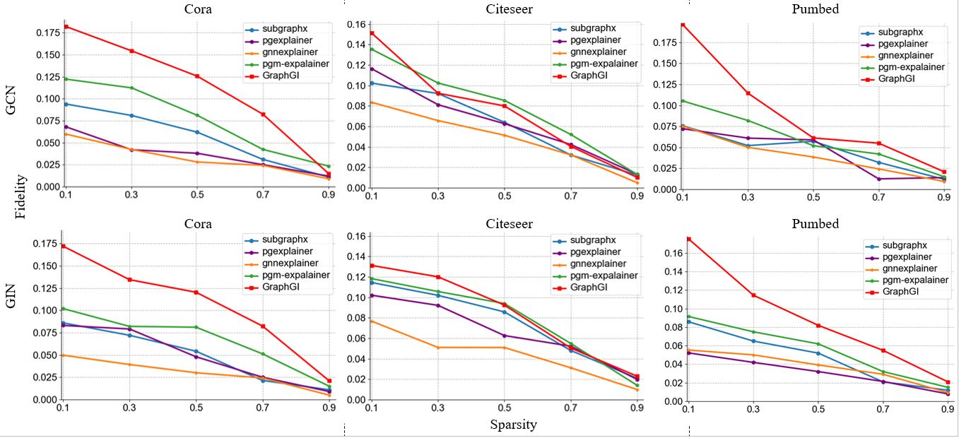
Figure 3: The fidelity scores, derived from the application of the GCN and GIN model on various real-world datasets.

Table 7: Comparison of computational times (Unit: seconds)

	BA-shapes	BA-community	Tree-cycle	Tree-grid	Cora	Citeseer	Pubmed
# No sample	4349	5149	1202	2103	48242	OOM	OOM
# Sample	502	519	51	135	3154	3527	6420

5.6 Experimental Result

5.6.1 Explanation on Syntheic datasets

In the synthetic datasets we have selected, the labels of the nodes are determined by motifs, which are considered the ground truth. Utilizing these motifs, we conducted a qualitative assessment of our proposed algorithm, GraphGI. For each dataset, we have chosen a representative instance and visualized the explanations provided by GraphGI (Fig.2). In these visualizations, the largest node signifies the target node, and the subgraph connected by bold black edges represents the explanatory subgraph computed by GraphGI. As illustrated, GraphGI is capable of successfully identifying the “house" structure within the BA-Shapes and BA-Community datasets. Given that the experiment is designed to explain the 2-hop GCN, the search scope for the explanatory subgraph is confined to the 2-hop subgraph of the target node. This limitation has resulted in GraphGI’s incomplete recognition of the cyclic structures present in the Tree-Grid and Tree-Cycles datasets. However, it is evident from the figure that GraphGI has made the best effort to discern the structure of the motifs.

Table 3 and 4 present the Fidelity Scores and Sparsity Scores of multiple explanation methods across various datasets. These metrics are employed to assess the accuracy and conciseness of each method in the task of node classification. An ideal explanation should possess both high sparsity and fidelity.

Table 3 indicates that in the interpretation of two-layer GCNs, GraphGI achieved the best fidelity and sparsity on the BA-shapes, BA-community and Tree-Grid datasets, and also demonstrated good performance on other datasets. In experiments, GraphGI has demonstrated an extremely high level of sparsity, a characteristic largely determined by the intrinsic properties of the data. In synthetic datasets, each undirected edge is actually represented by two directed edges. According to our subgraph search algorithm, the majority of the edges in the generated subgraphs are single directed edges. In contrast, other methods typically construct explanatory subgraphs by connecting important nodes, in other words, the edges in their explanatory subgraphs are composed of two directed edges. This methodological difference leads to GraphGI’s superiority in sparsity compared to other approaches. In short, the algorithmic design of GraphGI and the characteristics of the data work in concert, enabling it to produce sparser but effective subgraphs when processing synthetic datasets.

In Table 4, concerning the GIN model, GraphGI shows more stable and superior results, achieving the best fidelity and sparsity in the BA-shapes and Tree-cycles datasets, and also obtaining the best fidelity in the BA-community dataset. SubraphX and PGExplainer exhibited lower sparsity in both sets of experiments, which may be due to their lack of consideration for the interactions between data features and the continuous process of model decision-making during the computation, thus reducing the conciseness of the explanations.

5.6.2 Explanation on Real-world dataset

For real-world datasets, we still evaluate using fidelity and sparsity as metrics. Tables 5 and 6 present the Fidelity Scores and sparsity scores of multiple explanation methods across different datasets. It is worth noting that in the last row of Tables 5 and 6, we have marked the accuracy of the model training, which is due to the fact that we only considered the structural information of the graph data, differing from models that generally take into account data features. It can be observed that even with real-world datasets, our proposed GraphGI can maintain high fidelity and sparsity, indicating its effectiveness for such datasets. Additionally, it is noticeable that SubgraphX exhibits high sparsity, which is due to the inherent limitations of the algorithm leading to the selection of fewer edges. Furthermore, the selection of a smaller number of test points for explanation makes it possible to use SubgraphX and GraphGI. In fact, due to the complexity of the algorithms, it is challenging to apply them to large-scale graph-based real-world datasets, which will be the direction of our future research.

To validate the effectiveness of our proposed model, we conducted experiments using real-world datasets. By controlling the sparsity, we verified the proposed model’s quantities. Fig. 3 shows the performance of baselines under different sparsity levels. On the Cora and CiteSeer datasets, GraphGI demonstrated better performance, indicating that even in complex real-world graphs, our model can still capture substructures with the highest interactions. Moreover, we observed that our model outperformed others even at high sparsity levels, suggesting that the model can identify significant interaction structures within smaller graph structures. In Citeseer dataset, the subgraphs still contained a large number of edges, making the interactions between graph data structures very complex, which indirectly led to the degraded performance of the GraphGI model. This also suggests that greedy strategy-based models are challenging to apply to large-scale graphs. For the same reason, SubgraphX and PGExplainer showed poorer performance on real datasets. In summary, GraphGI can still ensure interpretability and reliability in real-world datasets.

5.7 Time Optimization Comparison

As previously mentioned, GraphGI is a greedy and computationally intensive explanation method. In order to enhance computational efficiency, we opted to employ a sampling approach to optimize its calculations. Table 7 illustrates the computational speed before and after the implementation of the sampling method for the first 20 test nodes. The results demonstrate that the use of the sampling method effectively improves computational efficiency and reduces calculation time.

6 Conclusion

The aim of this paper is to improve the interpretability of graph models by employing game-theoretic interaction. Specifically, diverging from the current Shapley-based approaches, this research endeavors to achieve the aforementioned objective by developing an explanation method that capitalizes on the interactions among data features, known as GraphGI. It simultaneously considers the positive and negative interactions across various data structures, utilizing a game-theoretic interaction mechanism to attribute explanations to the input data. The extensive experimental outcomes have substantiated the superiority of the proposed method when compared to other cutting-edge models and conventional baseline methods. This may indeed be a productive pathway for future studies focused on graph interpretation tasks.

References

- [1] Hao Yuan, Haiyang Yu, Shurui Gui, and Shuiwang Ji. Explainability in graph neural networks: A taxonomic survey. IEEE transactions on pattern analysis and machine intelligence, 45(5):5782–5799, 2022.
- [2] Federico Baldassarre and Hossein Azizpour. Explainability techniques for graph convolutional networks. arXiv preprint arXiv:1905.13686, 2019.
- [3] Federico Baldassarre and Hossein Azizpour. Explainability techniques for graph convolutional networks. arXiv preprint arXiv:1905.13686, 2019.
- [4] Dongsheng Luo, Wei Cheng, Dongkuan Xu, Wenchao Yu, Bo Zong, Haifeng Chen, and Xiang Zhang. Parameterized explainer for graph neural network. Advances in neural information processing systems, 33:19620–19631, 2020.
- [5] Phillip E Pope, Soheil Kolouri, Mohammad Rostami, Charles E Martin, and Heiko Hoffmann. Explainability methods for graph convolutional neural networks. In Proceedings of the IEEE/CVF conference on computer vision and pattern recognition, pages 10772–10781, 2019.
- [6] Zhitao Ying, Dylan Bourgeois, Jiaxuan You, Marinka Zitnik, and Jure Leskovec. Gnnexplainer: Generating explanations for graph neural networks. Advances in neural information processing systems, 32, 2019.
- [7] Hao Yuan, Haiyang Yu, Jie Wang, Kang Li, and Shuiwang Ji. On explainability of graph neural networks via subgraph explorations. In International conference on machine learning, pages 12241–12252. PMLR, 2021.
- [8] Minh Vu and My T Thai. Pgm-explainer: Probabilistic graphical model explanations for graph neural networks. Advances in neural information processing systems, 33:12225–12235, 2020.
- [9] Wenqian Li, Yinchuan Li, Zhigang Li, Jianye Hao, and Yan Pang. Dag matters! gflownets enhanced explainer for graph neural networks. arXiv preprint arXiv:2303.02448, 2023.
- [10] Hao Yuan, Jiliang Tang, Xia Hu, and Shuiwang Ji. Xgnn: Towards model-level explanations of graph neural networks. In Proceedings of the 26th ACM SIGKDD international conference on knowledge discovery & data mining, pages 430–438, 2020.
- [11] Ataollah Kamal, Céline Robardet, and Marc Plantevit. Game theoretic explanations for graph neural networks.
- [12] Selahattin Akkas and Ariful Azad. Gnnshap: Scalable and accurate gnn explanation using shapley values. In Proceedings of the ACM on Web Conference 2024, pages 827–838, 2024.
- [13] Alexandre Duval and Fragkiskos D Malliaros. Graphsvx: Shapley value explanations for graph neural networks. In Machine Learning and Knowledge Discovery in Databases. Research Track: European Conference, ECML PKDD 2021, Bilbao, Spain, September 13–17, 2021, Proceedings, Part II 21, pages 302–318. Springer, 2021.
- [14] Andrea Mastropietro, Giuseppe Pasculli, Christian Feldmann, Raquel Rodríguez-Pérez, and Jürgen Bajorath. Edgeshaper: Bond-centric shapley value-based explanation method for graph neural networks. Iscience, 25(10), 2022.
- [15] Shichang Zhang, Yozen Liu, Neil Shah, and Yizhou Sun. Gstarx: Explaining graph neural networks with structure-aware cooperative games. Advances in Neural Information Processing Systems, 35:19810–19823, 2022.
- [16] Lloyd S Shapley. Notes on the n-person game—ii: The value of an n-person game. 1951.
- [17] Hao Zhang, Yichen Xie, Longjie Zheng, Die Zhang, and Quanshi Zhang. Interpreting multivariate shapley interactions in dnns. In Proceedings of the AAAI Conference on Artificial Intelligence, volume 35, pages 10877–10886, 2021.
- [18] Wanyu Lin, Hao Lan, and Baochun Li. Generative causal explanations for graph neural networks. In International Conference on Machine Learning, pages 6666–6679. PMLR, 2021.
- [19] Phillip E Pope, Soheil Kolouri, Mohammad Rostami, Charles E Martin, and Heiko Hoffmann. Explainability methods for graph convolutional neural networks. In Proceedings of the IEEE/CVF conference on computer vision and pattern recognition, pages 10772–10781, 2019.
- [20] Thomas Schnake, Oliver Eberle, Jonas Lederer, Shinichi Nakajima, Kristof T Schütt, Klaus-Robert Müller, and Grégoire Montavon. Higher-order explanations of graph neural networks via relevant walks. IEEE transactions on pattern analysis and machine intelligence, 44(11):7581–7596, 2021.
- [21] Qiang Huang, Makoto Yamada, Yuan Tian, Dinesh Singh, and Yi Chang. Graphlime: Local interpretable model explanations for graph neural networks. IEEE Transactions on Knowledge and Data Engineering, 2022.
- [22] Yue Zhang, David Defazio, and Arti Ramesh. Relex: A model-agnostic relational model explainer. In Proceedings of the 2021 AAAI/ACM Conference on AI, Ethics, and Society, pages 1042–1049, 2021.
- [23] Thorben Funke, Megha Khosla, Mandeep Rathee, and Avishek Anand. Z orro: Valid, sparse, and stable explanations in graph neural networks. IEEE Transactions on Knowledge and Data Engineering, 2022.
- [24] Shurui Gui, Hao Yuan, Jie Wang, Qicheng Lao, Kang Li, and Shuiwang Ji. Flowx: Towards explainable graph neural networks via message flows. IEEE Transactions on Pattern Analysis and Machine Intelligence, 2023.
- [25] Michael Sejr Schlichtkrull, Nicola De Cao, and Ivan Titov. Interpreting graph neural networks for nlp with differentiable edge masking. arXiv preprint arXiv:2010.00577, 2020.
- [26] Amirata Ghorbani and James Zou. Data shapley: Equitable valuation of data for machine learning. In International conference on machine learning, pages 2242–2251. PMLR, 2019.
- [27] Benedek Rozemberczki, Lauren Watson, Péter Bayer, Hao-Tsung Yang, Olivér Kiss, Sebastian Nilsson, and Rik Sarkar. The shapley value in machine learning. arXiv preprint arXiv:2202.05594, 2022.
- [28] Michel Grabisch and Marc Roubens. An axiomatic approach to the concept of interaction among players in cooperative games. International Journal of game theory, 28:547–565, 1999.
- [29] Zhilin Yang, William Cohen, and Ruslan Salakhudinov. Revisiting semi-supervised learning with graph embeddings. In International conference on machine learning, pages 40–48. PMLR, 2016.
- [30] Thomas N Kipf and Max Welling. Semi-supervised classification with graph convolutional networks. arXiv preprint arXiv:1609.02907, 2016.
- [31] Keyulu Xu, Weihua Hu, Jure Leskovec, and Stefanie Jegelka. How powerful are graph neural networks? arXiv preprint arXiv:1810.00826, 2018.