Why collective behaviours self-organise to criticality: A primer on information-theoretic and thermodynamic utility measures

Abstract

Collective behaviours are frequently observed to self-organise to criticality. Existing proposals to explain these phenomena, such as Self-organised Criticality (SOC), are fragmented across disciplines and only partially answer the question. This paper investigates the underlying, intrinsic, utilities that may explain self-organisation of collective behaviours near criticality. We focus on information-driven approaches such as predictive information, empowerment, and active inference, as well as thermodynamic efficiency, which incorporates both information-theoretic and thermodynamic quantities. By interpreting the Ising model as a perception-action loop, we compare how different intrinsic utilities shape collective behaviour and analyse the distinct characteristics that arise when each is optimised. In particular, we highlight that at the critical regime thermodynamic efficiency balances the predictability gained by the system and its energy costs. Finally, we propose the Principle of Super-efficiency, suggesting that collective behaviours self-organise to the critical regime where optimal efficiency is achieved with respect to the entropy reduction relative to the thermodynamic costs.

I Introduction

Self-organisation is a process where a system spontaneously develops new structured patterns or functions, without being explicitly controlled by an external force. This process is observed in a wide range of natural and artificial systems, where local interactions among components generate global order. As a fundamental concept in complexity science, self-organisation is extensively studied in various disciplines, including systems theory, condensed matter physics, systems biology, as well as social sciences.

From a physics perspective, self-organisation is generally viewed as entropy reduction or increase in order in an open system “without specific interference from outside” [1, 2]. From a biological perspective, self-organisation is typically defined as a pattern-formation process that relies entirely on interactions among the lower-level components of the system [3]. There are three key aspects to self-organisation [1, 4, 3, 2, 5]:

1. Spontaneous order: the system evolves into a more organised state without external control;

2. Emergence of coherent global behaviour: there is an observable transition to a more coherent collective behaviour;

3. Local interactions and long-range correlations: system components operate on local information but exhibit long-range interaction and connectivity.

One of the underlying principles for the spontaneous order created in self-organisation, as suggested by Kauffman [4], is the “constraint closure”, which means that the system carries out some work to create constrains on the release of energy, and those constraints, in turn, channel the energy to perform more useful work. Thus, a successful framework describing self-organisation needs to account for thermodynamic characteristics of the spontaneous order, capturing the corresponding energy flows and costs.

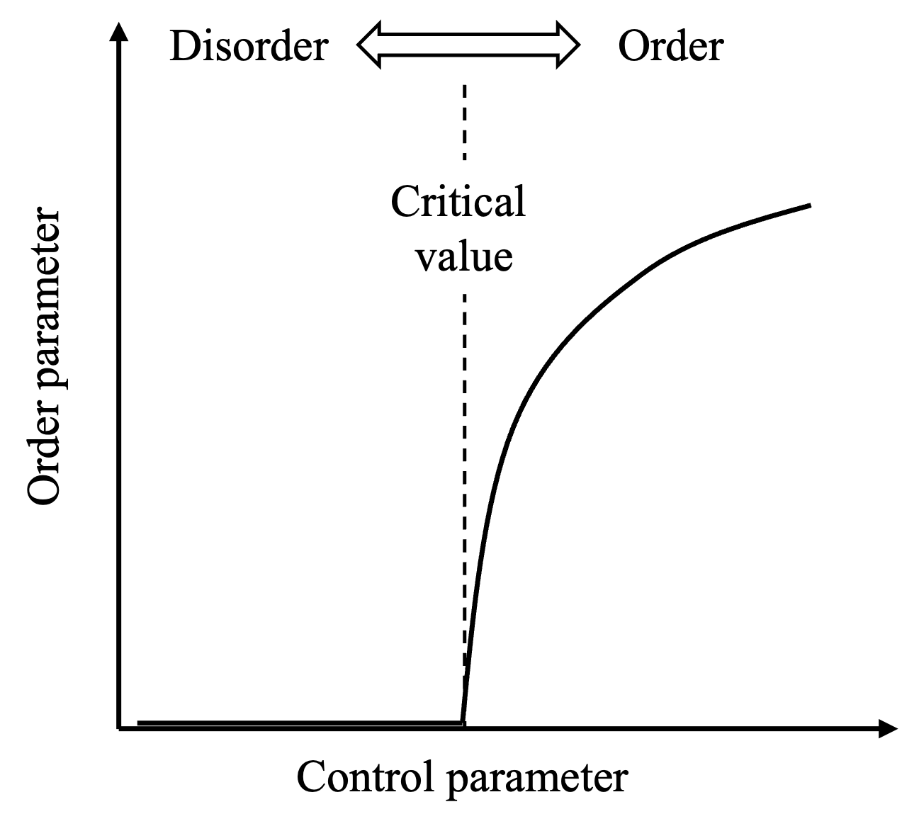
(a) Order-disorder phase transition

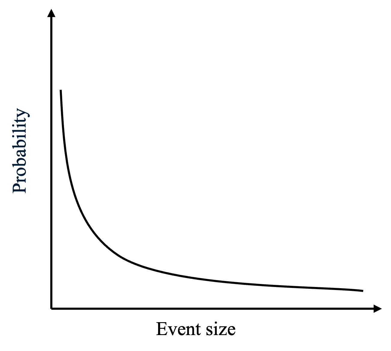
(b) Power-law distribution of event sizes

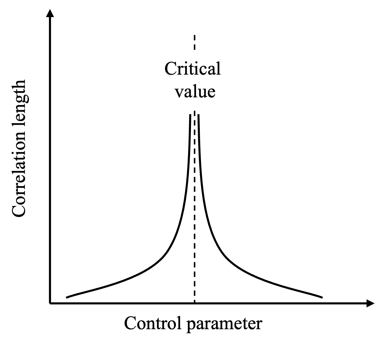
(c) Divergence of correlation length

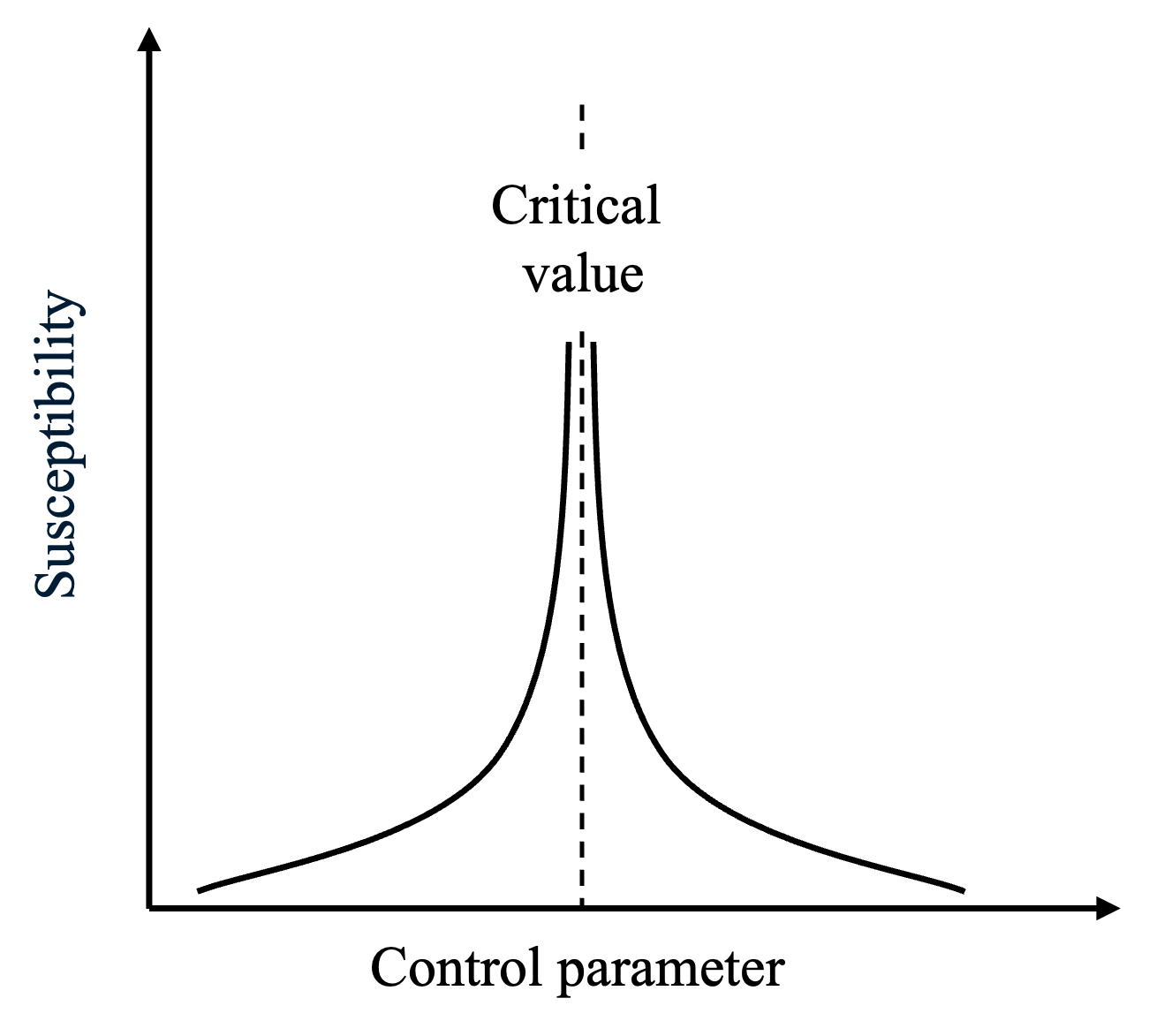
(d) Divergence of susceptibility

Figure 1: Schematic representations for second order phase transition and critical phenomena. The control parameter is a variable that influences the state of the system, such as temperature or pressure, while the order parameter quantifies the degree of order within the system, with non-zero value only in the ordered phase. (a) Order parameter changes continuously in response to changes in the control parameter during a second-order phase transition. (b) Scale-invariance observed at the critical regime indicates a power-law distribution of event sizes, e.g. avalanche or earthquake magnitudes. (c) Correlation length diverges at the critical point, facilitating long-range correlation of fluctuations between constituent parts of the system. (d) Susceptibility diverges at the critical point, reflecting the system’s increased sensitivity to external perturbations.

Typically, self-organised collective behaviours, such as magnetisation, ant colony foraging, swarming, slime mould aggregation, flocking of birds, and neural processing in the brain, exhibit critical phenomena [6, 7, 8, 9, 10, 11, 12, 13, 14]. These phenomena occur at the critical point of a continuous phase transition, and include scale-invariance [15], divergence of correlation length, and divergence of the response function [16]. These hallmarks are observed in physical [17, 18], biological [7, 11, 19], social[20, 21] and hybrid systems [22].

Scale-invariance means that the system near the critical regime does not exhibit a typical length scale, i.e., patterns appear similar on many magnification levels. Consequently, the size of events at criticality follows a power-law distribution. The correlation length measures the scale on which fluctuations or changes at one point in the system affect those at another point, and the divergence of this quantity implies the long-range interaction between constituent components of the system. In the context of collective systems such as groups of biological organisms, long-range interactions may generate more coherent global behaviour for the group. The response function characterises the system’s response to perturbations. For example, magnetic susceptibility represents the change of magnetisation of a material in response to an applied magnetic field, and is known to diverge at criticality, as even a small field can induce large changes in magnetisation. At the critical regime, systems typically become highly sensitive to small changes in parameters, showing large responses to minor perturbations. Another implication to collective behaviour in biological systems is that the groups may become more sensitive to stimuli from the external environment, such as detection of predators.

Physical systems, such as fluids or magnets, can be driven to criticality by adjusting a control parameter, e.g., temperature or pressure, that influences the state of the system. As the control parameter reaches a critical value, the order parameter, which measures the degree of order or organisation within the system, undergoes a transition, e.g., from zero (disordered phase) to non-zero (ordered phase). However, for biological systems, there are typically no well-defined protocols to adjust the control parameters. Nevertheless, nature somehow finds its way to poise the system at or near criticality.

A canonical framework describing the mechanism behind such dynamics is the theory of Self-Organised Criticality (SOC), initially introduced by Bak et al. [23] based on a mathematical model known as the Bak–Tang–Wiesenfeld (BTW) Sandpile Model. Central to this theory is the interplay of two opposing forces that push a system to criticality. The first force is the driving force, characterised by gradual, incremental changes that increase the system’s energy, disorder, or stress (e.g., adding sand to a sand pile). When the accumulated stress or energy reaches a certain threshold, a stabilising force comes into play, triggering a response that dissipates or redistributes the energy, typically in a sudden and possibly widespread manner (e.g., sand avalanche). Under the influence of these two opposing forces, the system “evolves” to criticality and remains there. The concept of SOC inspired a series of studies that applied it to develop an understanding of the underlying mechanism that generates critical phenomena in various complex systems such as forest fires [24, 25, 26], earthquakes [27] and brain activities [7, 10, 28, 29]. However, it can be argued that SOC provides a possible explanation for how criticality occurs, rather than why it benefits the system.

In this work, we are interested in exploring the intrinsic utility for a self-organising system approaching and operating at the critical regime. Here, an intrinsic utility is understood broadly, as the inherent benefit or value gained by the system from its own organisation, independently of external rewards and objectives [30, 31]. Recent research on intrinsic utilities shaping self-organising behaviours primarily examined how systems, especially autonomous robots and biological entities, utilise task-independent objectives in order to optimise and adapt their behaviours. Notable strategies include predictive information maximisation [32, 33, 34, 35, 36, 37, 38], empowerment maximisation [39, 40, 41, 42, 43, 44], and free energy minimisation [45, 46, 47, 48, 49] (which encompasses both intrinsic and extrinsic utilities). A consistent feature of these approaches is their employment of information theory in quantifying the intrinsic motivation for the spontaneous order and emergence of collective behaviours. Informally, one identifies a change in suitably defined entropic quantities with relevant pattern formation at macro-level. Although these approaches can sometimes induce critical behaviours [36, 37, 38, 50], this outcome is not invariably guaranteed. Thus, to understand the fundamental drivers of critical phenomena in collective behaviours, it is essential to give a thermodynamic account of the intrinsic motivation.

The three frameworks mentioned above predominantly focus on the informational benefit (e.g., increase in predictability, order or potential influence, reduction in uncertainty or surprise) without explicitly addressing the associated energy costs. Although the free energy minimisation incorporates the term “energy” in its name, the utilised concept is an information-theoretic construct which does not align with the thermodynamic free energy (more details provided in Section IV). As a result, the trade-offs between informational benefits and thermodynamic costs are not captured explicitly.

In this work, we aim to formulate a unifying principle connecting (i) the intrinsic functional benefits of collective behaviour (measured as entropy reduction or gained predictability) and (ii) the associated thermodynamic costs. Studies of various complex dynamical systems such as urban growth [51], self-propelled particles [52], contagion network [53], and the canonical Curie-Weiss model for magnetisation [54], have shown that systems at critical points exhibit maximum thermodynamic efficiency defined as a ratio of the gained predictability (i.e., reduction in uncertainty, or the increase in the internal order) to the amount of work required to change the underlying control parameter. These studies strongly suggested that the rate of entropy reduction relative to the carried-out work diverges (peaks in finite systems) at critical points.

We argue that these studies exemplify a general principle of super-efficiency: at the critical regime, a self-organising system of interacting agents achieves the optimal thermodynamic efficiency by gaining maximal predictability of collective behaviour per unit of the expended work. Informally, one can say that a complex system finds the regime where the cost of “keeping it together” is justified. On one hand, given some available energy to change the control parameter, the system identifies the control parameter value where the gain in predictability maximises. On the other hand, given a required predictability gain, the system finds the point (the value of the control parameter) where the energy cost associated with the change would be minimal. The principle of super-efficiency suggests that this point aligns with the critical point.

This principle encapsulates the intrinsic utility of self-organising collective behaviour, elucidating why some systems gravitate towards criticality. Our discussion will begin with a background on criticality and phase transitions provided in Section II. Section III outlines the notations and essential technical preliminaries. Section IV provides an overview of established intrinsic utility approaches, while Section V describes thermodynamic efficiency defined at the intersection of information theory and thermodynamics. A common example using the two-dimensional Ising model is presented in Section VI to compare the self-organising behaviours driven by different intrinsic utilities. Section VII offers a more in-depth discussion on the principle of super-efficiency, and Section VIII summarises the findings and presents the final conclusion. This study offers insights into the distinct characteristics of collective behaviour derived within each framework, and emphasises how the principle of super-efficiency captures the intrinsic utility for collective behaviour at the critical regime.

II Phase transitions and criticality

Generally, there are two types of phase transitions: first-order phase transition, characterised by discontinuity in the system’s order parameter during the transition, and second-order phase transition, where the order parameter changes smoothly and continuously. Critical phenomena are observed in second-order phase transitions.

The percolation model serves as a canonical example for understanding phase transition and criticality [55, 15]. Let us consider an infinite-size lattice where each site can either be vacant or occupied. In the simplest version, each site is independently occupied with a probability $p$, leading to the formation of clusters of connected occupied sites. A percolating cluster is a group of connected occupied sites that span across the lattice from one side to the opposite. The percolation phase transition is often studied by tracing percolating cluster sizes with respect to the control parameter $p$ (the site occupancy probability), and one can distinguish between:

• Largest cluster size (LCS): a low LCS value indicates a more disordered state where most clusters are small, while a high LCS value indicates a more ordered state where majority of the sites belong to the same cluster;

• Average cluster size (ACS) measures the average cluster size excluding the percolating cluster. This quantity corresponds to the initial susceptibility in the scaling theory for magnetic systems [56, 57].

The divergence of ACS at the critical point can be understood as follows: at low $p$, predominantly small clusters form, resulting in a small ACS. It increases with $p$ until the percolation threshold $p_{c}$ is reached. At $p=p_{c}$, a percolating cluster forms for the first time, spanning the entire lattice, and the ACS diverges. Beyond $p_{c}$, smaller clusters are progressively absorbed by the giant percolating cluster as more sites become occupied. The absorption reduces the average size of the remaining finite clusters, causing the ACS to decrease.

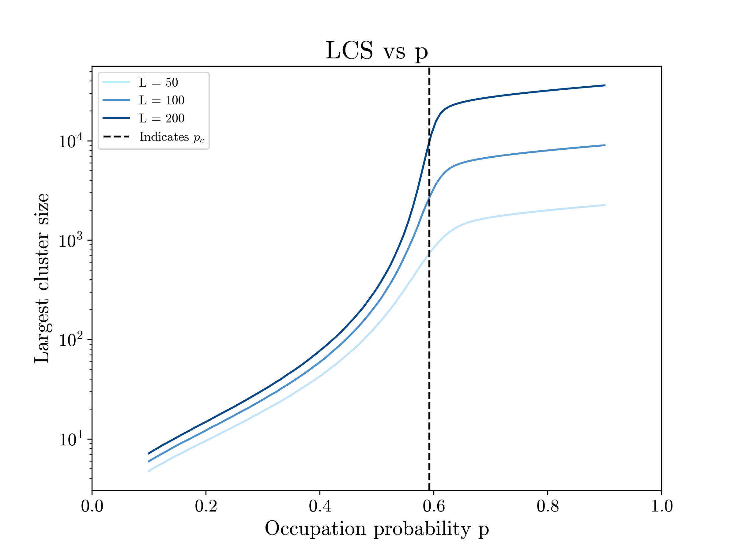
(a) Order-disorder phase transition (largest cluster size)

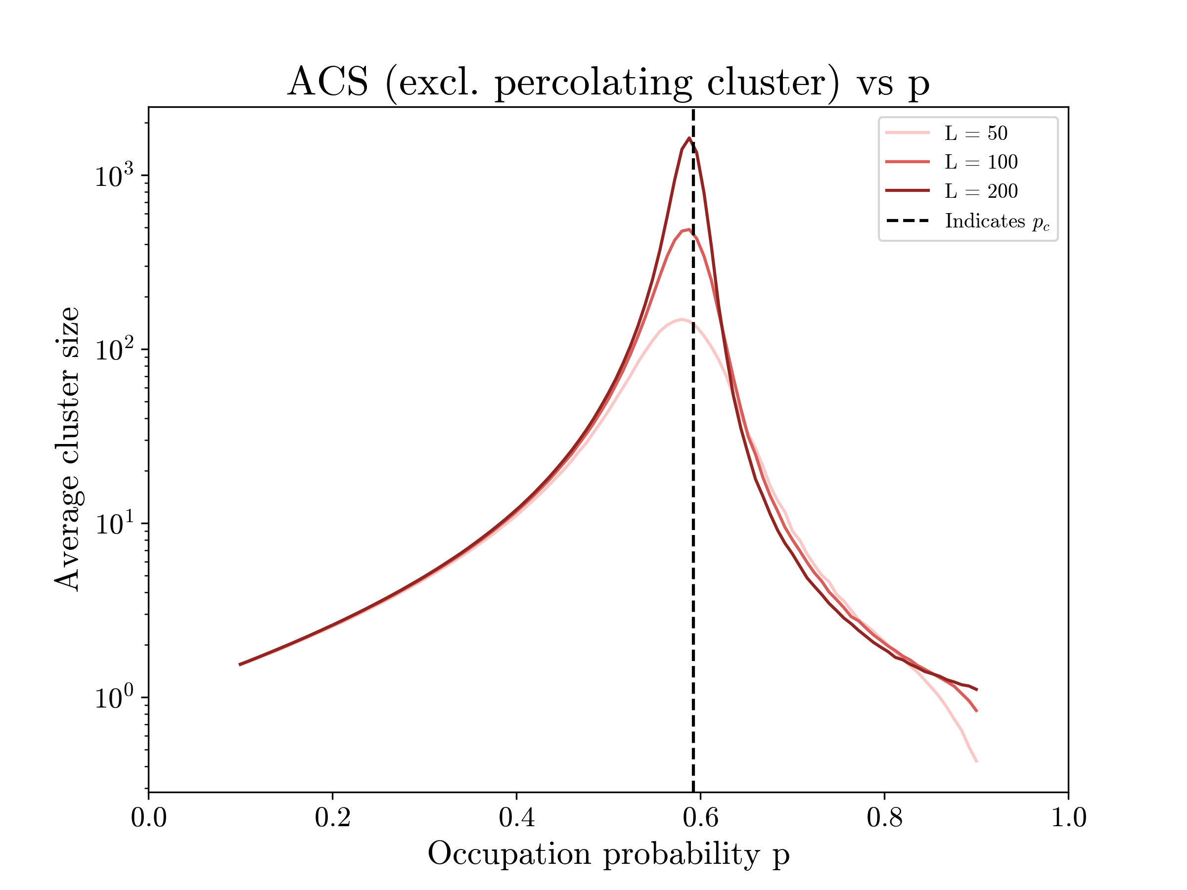
(b) Divergence of susceptibility (average cluster size)

Figure 2: Site percolation model: largest cluster size and average cluster size (excluding percolating cluster) simulated for different lattice sizes $L$ [58]. Vertical axis in log-scale.

Similarly, the correlation length $\xi$ also diverges at the critical point. The divergence of $\xi$ indicates that fluctuations at one single site can propagate infinitely far across the system, reflecting extensive long-range interactions throughout the lattice at the critical regime.

The relationship between average cluster size $\langle S\rangle$ or correlation length $\xi$ and the control parameter $p$ at the critical regime can be expressed as:

$$\langle S\rangle \propto|p-p_{c}|^{-\gamma}$$ (1)

$$\xi \propto|p-p_{c}|^{-\nu}$$ (2)

where $\gamma,\nu$ are critical exponents, positive numbers whose value depends on the dimension of the system. Put simply, at criticality, the system is very sensitive to small perturbations.

The critical phenomena observed in the lattice model provide insights into the dynamics of collective behaviour near the critical point. Structurally, a percolating cluster spanning the entire lattice forms when the control parameter reaches its critical value. Functionally, the system demonstrates a heightened responsiveness to changes in control parameters, exhibiting long-range correlations between its constituents, characterised by the divergence of average cluster size and correlation length. The ability to propagate information over long distances and maximise responsiveness enables more coherent global behaviour and enhances the collective group’s sensitivity to external changes, thus offering advantages for the system to operate at or near the critical regime.

The ubiquity of critical phenomena in nature led to vigorous research into potential mechanisms generating criticality. In the 1980s, the theory of Self-Organised Criticality (SOC) was proposed by Bak, Tang and Wiesenfeld [23] as a possible explanation. Under SOC, specific dissipative dynamical systems naturally evolve towards criticality regardless of their initial states. At the core of the SOC models is the presence of a slow driving force that pushes a subcritical system towards critical or supercritical state, and a fast regulating force that brings the system back from supercritical states. The driving force permits the build-up of energy that is later released by the regulating force, propagating throughout the system via localised interactions.

One of the classical SOC models is the Drossel and Schwabl forest-fire model [24, 25], which enhances the percolation model. Let the occupied sites represent trees grown in the forest. Additionally, the model includes another dynamics: lightning strikes a random site with a probability of $f$. At each time step, the lattice sites are updated based on four rules:

1. on an empty site, a tree grows with probability $p$;

2. lightning strikes a random site in the forest with probability $f$, turning a tree into a burning tree;

3. a tree burns if at least one of its adjacent neighbours is burning;

4. a burning tree turns into an empty site, and the model runs indefinitely.

Following the above rules, as trees grow, they form clusters that contribute to propagation of forest fires. The tree growth probability at any given site mirrors the site occupancy probability in the percolation model. Lightning acts as an external factor that regulates tree growth. While the percolation model requires a manual adjustment of $p$ to reach the critical point, the dynamics of the DS forest-fire model self-regulates to criticality. Thus, critical phenomena, such as long-range correlations and scale-invariance, are considered to be self-organising in response to the model’s inherent dynamics.

The system’s behaviour is governed by two opposing forces: lightning strikes and tree growth. When trees are sparse, the chance of them getting hit by a lightning strike is low; therefore, trees continue to grow. When tree density goes beyond the critical density, giant clusters form, spanning the entire lattice. A lightning strike on such a cluster results in a fire that consumes the entire cluster, returning the system to a subcritical state. The system approaches a steady state at the critical point under the influence of these two forces, where the fire event sizes follow a power-law distribution and the correlation length $\xi$ diverges (Figure 3).

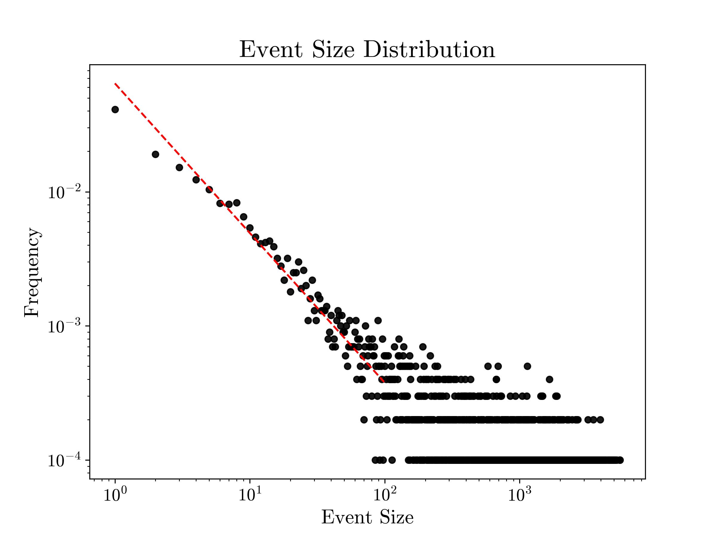
(a) Power-law distribution of event sizes

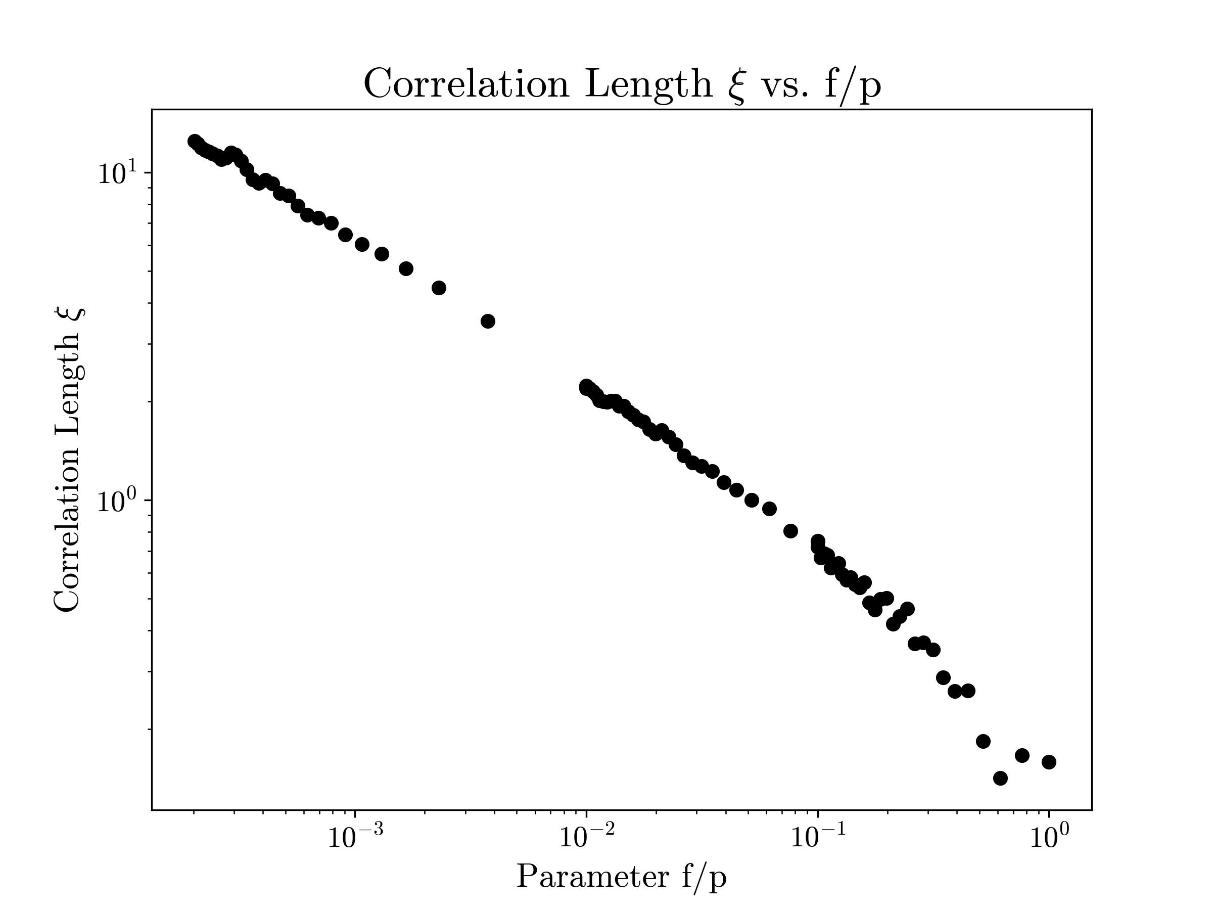
(b) Divergence of correlation length

Figure 3: DS forest-fire model: event size distribution and correlation length plots (log-log scale), simulated on a 100$\times$100 square lattice [58]. Critical point occurs in the limit $f/p\rightarrow 0$ [25].

The dynamic process that drives the system to the critical point hinges on the condition of “separation of time scales”. This condition specifies that the time required to burn down the whole cluster is much shorter than the time it takes to grow a tree, which in turn is much shorter than the time between two lightning strikes at the same site. This condition translates to a slow dynamic of the external driving force (the lightning) and a fast dynamic of local interaction (fire spreading and tree burning). It ensures that (1) no trees grow during a burn, and (2) there is a substantial energy accumulation between lightning events, leading to the destruction of many trees by a single lightning strike [24].

There is an ongoing debate regarding the characteristics of the power-law distribution and criticality generated by the forest fire model or SOC models in general. For example, numerical results indicate that the scaling law observed in the forest-fire model is transient and does not hold at larger scales [59]. Findings of [60] challenge the view that SOC systems inherently exhibit exact critical scaling, but suggest that the forest-fire model demonstrates weak criticality — a concept that is based only on the way that correlation length diverges, without the requirement for an exact power law distribution.

The theory of Self-Organised Criticality elucidates the mechanism behind self-regulation of the dynamics towards a critical point where scale-invariance and long-range correlations may induce collective behaviours. However, SOC does not explain what intrinsic utility is attained by the collective behaviour of the system operating at the critical regime. The subsequent sections will review several approaches that explore the issue of intrinsic motivations.

III notations and Technical Preliminaries

III.1 Notations

Here we offer a brief summary of the notation conventions adopted in this work. Detailed explanations of these notations will be provided within their respective contexts:

• Capital letters $W,S,A,M$… for random variables;

• Small letters $w,s,a,m$… for a realisation of the corresponding random variable;

• Letters $\mathcal{I},\mathfrak{E},\mathcal{F}$ for quantities computed using the information-theoretic approaches, corresponding to predictive information, empowerment and variational free energy, respectively;

• Blackboard bold font $\mathbb{E},\mathbb{S},\mathbb{F},\mathbb{W},\mathbb{Q},\mathbb{I}$ for thermodynamic quantities or statistical quantities, corresponding to energy, entropy, thermodynamic free energy, work, heat and Fisher information respectively.

Additionally, we adopt the notation where subscript $x_{t}$ denotes the state at time $t$ in a time series, and superscript $x^{(i)}$ indicates the $i^{th}$ instance in the population.

III.2 Information-theoretic quantities

We begin by introducing standard notations for information-theoretic quantities that are relevant to the subsequent sections. For readers interested in more details, please refer to [61].

For a discrete random variable $X$ that has probability mass function $p(x)=Pr\{X=x\}$, the entropy $H(X)$ which measures the uncertainty of random variable $X$ is defined as:

$$H(X)=-\sum_{x}p(x)\log p(x)$$ (3)

where by convention, base 2 logarithms are used throughout this paper, and the resulting unit is in bits.

If a pair of discrete random variables $(X,Y)$ follows joint probability distribution be $p(x,y)$, the conditional entropy $H(Y|X)$ is defined as:

$$H(Y|X)=-\sum_{x}\sum_{y}p(x,y)\log p(y|x)$$ (4)

The conditional entropy $H(Y|X)$ measures the remaining uncertainty in random variable $Y$ given the knowledge of random variable $X$.

The mutual information between two discrete random variables $X$ and $Y$ is defined as:

$$I(X;Y)=\sum_{x}\sum_{y}p(x,y)\log\frac{p(x,y)}{p(x)p(y)}$$ (5)

Mutual information is the reduction in surprise about one random variable given the knowledge of the other. It is symmetrical and can be expressed as the difference between entropy and conditional entropy:

$$I(X;Y)=H(X)-H(X|Y)=H(Y)-H(Y|X)$$ (6)

The relative entropy or Kullback–Leibler divergence between two probability mass functions $p(x)$ and $q(x)$ is defined as:

$$D(p||q)=\sum_{x}p(x)\log\frac{p(x)}{q(x)}$$ (7)

The KL divergence $D(p||q)$ quantifies how much information is lost when an alternative probability distribution $q(x)$ is assumed as a model instead of the actual distribution $p(x)$.

IV Information-driven self-organisation

Information-driven self-organisation is an active area of research that applies information theory to study the behaviours of an agent or a group of agents. The information-theoretic utility functions used to derive the behaviours have the advantage of being universal and domain-invariant. These measures are considered strong candidates for capturing the informational benefit of increased order in collective systems. Two broad categories can be identified: purely intrinsic, and “hybrid” measures which incorporate, in addition, an extrinsic target or preference.

IV.1 The perception-action loop

Approaches formalising information-driven self-organisation typically assume an underlying model of agent-world interaction. This interaction is generally modelled with a perception-action (or sensorimotor) loop, using random variables to reflect the probabilistic nature of the dynamic. Figure 4 illustrates the causal network of the perception-action loop traced over time, where $W_{t}$, $S_{t}$, $A_{t}$, $M_{t}$ represent the state of the world, the sensor, the actuator and memory (the controller) at time $t$. The perception-action loop captures the following dynamics:

• At any given time $t$, the world state $W_{t}$ leads to an update of the agent’s sensory state $S_{t}$. The mapping from $W$ to $S$ is specified by kernel $\beta:W\rightarrow S$, representing the agent’s sensory mechanism;

• The agent’s memory (or controller) $M_{t}$ is influenced by both memory from the previous time step $M_{t-1}$ and the current sensory $S_{t}$, a relationship represented by kernel $\phi:M\times S\rightarrow M$;

• Depending on the memory state, the agent updates its action $A_{t}$ according to the policy $\pi:M\rightarrow A$. $M_{t}$ also carries through to the future $M_{t+1}$.

• The action $A_{t}$ and the world state $W_{t}$ jointly update the next world state $W_{t+1}$. The mapping is specified by kernel $\alpha:W\times A\rightarrow W$, representing the agent’s actuation mechanism.

It is worth noting that $\alpha$ and $\beta$ are kernels that capture the agent’s embodiment in terms of the agent’s sensor and actuator capabilities. They set constraints to how the agent may explore the environment, act and learn [62, 63].

Figure 4: Causal structure of perception-action loop of an agent with memory, traced over time.

In the next subsections, we will elaborate on the variations of causal network representations within different intrinsic utility frameworks. A common example will be presented in section VI.

IV.2 Intrinsic utility approaches

The notion of “intrinsic utility” suggests that the utility provided to the agent is internal and task-independent [64, 30]. Predictive information maximisation [32, 33, 34, 35, 36, 37, 38] and empowerment maximisation [39, 40, 41, 42, 43, 44] are two important approaches that utilise information-theoretic measures as intrinsic motivation for inducing self-organising behaviours.

IV.2.1 Predictive information

Predictive information [65], also known as effective measure complexity [66] or excess entropy [67], measures how much the observed history reduces uncertainty about the future. In the context of robotic behaviour development, predictive information in the sensor space may serve as an objective function for behaviour learning. Predictive information maximisation has been implemented for memory-less agents [32, 33, 34, 35, 36, 37, 38] but potentially can be adapted to incorporate external memory. Figure 5 illustrates a reduced causal network for a simple memory-less agent (reactive control) on which predictive information is applied.

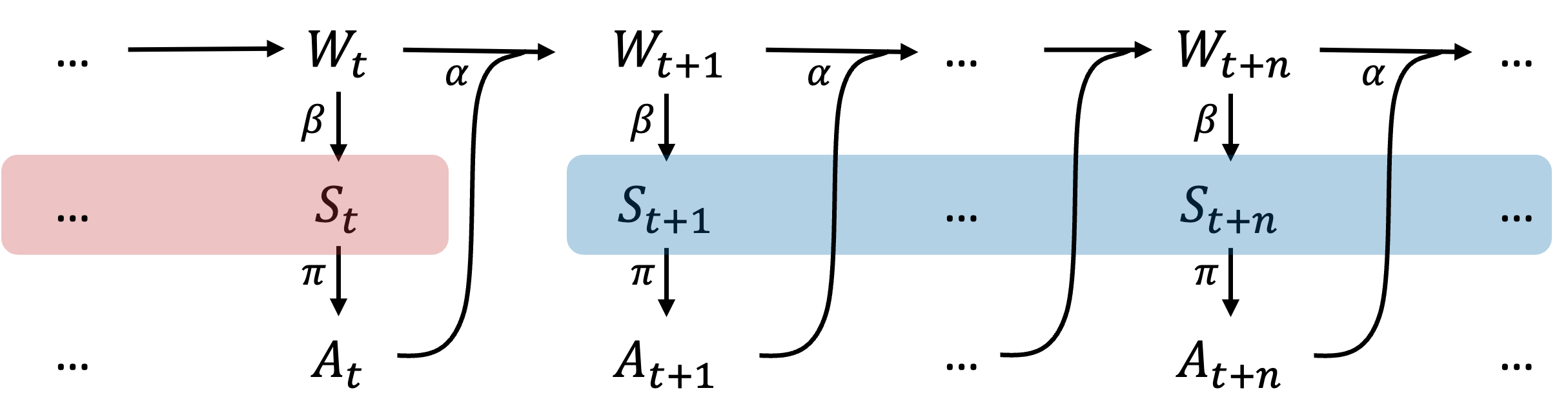
Figure 5: Causal structure of perception-action loop of a memory-less agent traced over time. Coloured blocks represent the two components that mutual information is calculated for predictive information.

Predictive information (used as intrinsic utility) is defined as the mutual information between past and future sensory states [32]. This can be further decomposed into components that represent the diversity and predictability [32, 5]:

$$\begin{split}\mathcal{I}:&=\quad I(S_{past};S_{future})\\ &=\underbrace{H(S_{future})}_{\text{Richness of future states}}-\underbrace{H(S_{future}|S_{past})}_{\text{Unpredictability of future}}\end{split}$$ (8)

Considering only one time step into the future, predictive information is defined as:

$$\mathcal{I}:=I(S_{t};S_{t+1})$$ (9)

Predictive information is measured in bits. Equation (8) indicates that predictive information is large when the entropy of the future sensory states $H(S_{future})$ is large, corresponding to a rich future experience, and/or when conditional entropy $H(S_{future}|S_{past})$ is small, representing a more predictable future. In both extremes, where there is complete order (no diversity) or complete randomness (no predictability), the predictive information will be zero.

The Venn diagram in Figure 6 illustrates the relationship between the time series of past and future sensory states. We note that conditional entropy $H(S_{past}|S_{future})$ represents the remaining entropy of historical sensory states given the future states, which is the part of history that we are unable to reconstruct using information from the future. For example, reconstructing the question given the answer to that question.

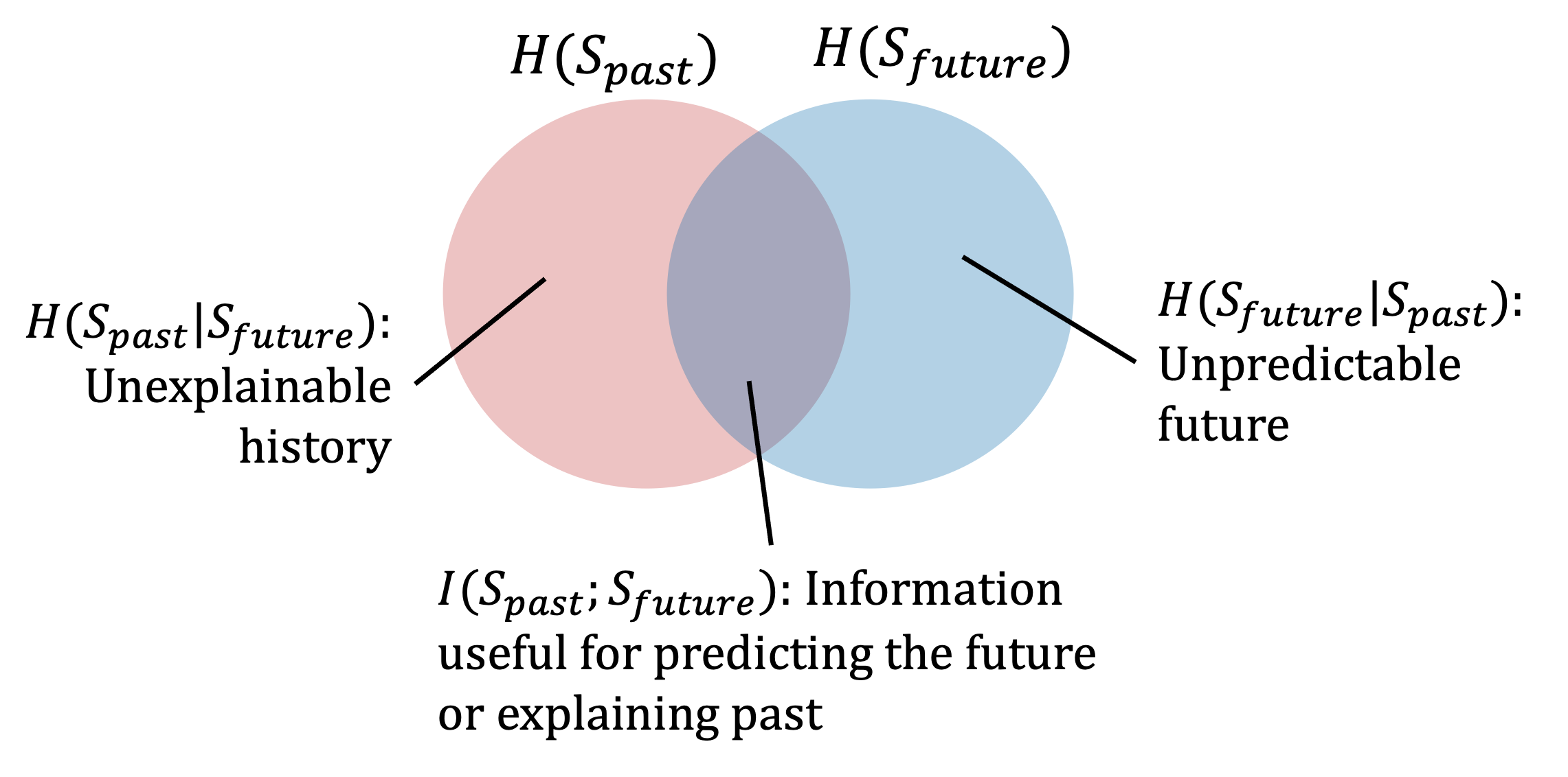
Figure 6: The Venn diagram of predictive information shown as the mutual information (the overlap area) between past and future sensory states: it represents how useful the past is for predicting the future.

Behavioural rules can be derived using the predictive information maximisation approach, forming a policy $\pi$ mapping sensory states to actions. Policy $\pi$ can be either deterministic, such as a simple mapping from sensor values to actions, or stochastic, which is represented by a conditional probability distribution $\pi\equiv p(a|s)$. The general form of the objective function for a one-step predictive information-driven agent is then expressed as:

$$\begin{split}\pi^{*}(a_{t},s_{t})&=\underset{\pi(a_{t},s_{t})}{\arg\max}\>\{\mathcal{I}\}\\ &=\underset{\pi(a_{t},s_{t})}{\arg\max}\>\{I(S_{t+1};S_{t})\}\end{split}$$ (10)

where $\pi^{*}$ denotes the optimal policy.

An agent motivated to maximise predictive information chooses policies that result in more diverse and, at the same time, predictable outcomes. In the context of collective behaviour, maximising predictive information has also been shown to induce cooperative behaviour under decentralised control [68, 34, 36]. The increase of predictive information differs from merely reducing randomness in the system; it enhances the richness of structure in the collective system. As shown in Section VI, collective behaviour resulting from maximising predictive information for each individual may appear random, but locally, it maintains a high level of diversity, aligned with the predictability of an individual’s sensory states.

IV.2.2 Empowerment

Alternatively, we can focus on a specific segment of the causal network that captures the influence of actions on subsequent sensory states through the external world (Figure 7). Empowerment measures this influence as the maximum amount of information an agent can inject from its actuators ($A$) to its sensors ($S$) at a future time via the environment.

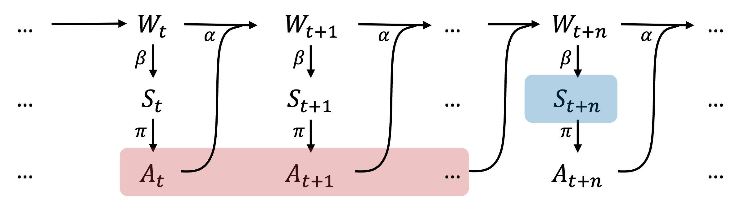
Figure 7: Causal structure of perception-action loop of a memory-less agent traced over time. Coloured blocks represent the components of mutual information which determines empowerment.

The n-step empowerment is defined as the Shannon channel capacity $C$ or maximum mutual information between the current sequence of actions $A_{t}^{n}=\{A_{t},A_{t+1},...,A_{t+n-1}\}$ and future sensor value $S_{t+n}$ [39]:

$$\begin{split}\mathfrak{E}:&=C(A_{t}^{n}\rightarrow S_{t+n})\\ &\equiv\max_{p(a_{t}^{n})}\>I(S_{t+n};A_{t}^{n})\end{split}$$ (11)

Empowerment is measured in bits. Considering only the most immediate future, one-step empowerment can be computed by:

$$\mathfrak{E}:=\max_{p(a_{t})}\>I(S_{t+1};A_{t})$$ (12)

The definition (12) is referred to as general or context-free empowerment since it measures only the agent’s general ability to inject information into its future sensory states. In order to use empowerment as the driver for an agent’s action, one needs to distinguish between different states of the environment, so that the agent can make decisions accordingly. This is achieved by context-dependent empowerment. The context refers to the state of the environment $w$ that affects the perception-action loop characteristic $p(s|a)$. More specifically, the future sensory state of the agent is affected by both its past actions and the historical states of the world. In other words, the same actions can lead to different distributions of future sensory states when the external environment has changed. Instead of considering a general action-perception characteristic $p(s|a)$, empowerment should be considered for a specific world state or context [39, 40, 43, 69]:

$$\mathfrak{E}(w_{t}):=\max_{p(a_{t}^{n}|w_{t})}\>I(S_{t+n};A_{t}^{n}|w_{t})$$ (13)

Given that an action $a_{t}$ stochastically leads to a collection of possible future world states $\Gamma$, the resulting average context-dependent empowerment is computed as:

$$\mathfrak{E}(W_{t}):=\sum_{w_{t}\in\Gamma}p(w_{t})\mathfrak{E}(w_{t})$$ (14)

This quantity can be used as an objective function for an empowerment-driven agent to make decisions on which action to take. More commonly, the state of the world $W$ would be replaced by some context $K$ that approximates it if the full world information is not available.

The general empowerment, as defined in equations (11) and (12), is different from the average context-dependent empowerment [43]. General empowerment does not consider the varying influence of actions in different states, since the channel capacity is computed using only $p(s|a)=\sum_{w}p(s|a,w)p(w)$. In contrast, the average context-dependent empowerment, as defined in equation (14), captures the nuanced ways in which different states can affect the actuation-sensing channel by computing $\max_{p(a|w)}\>I(S;A|w)$, and then average over all possible states.

The objective function for an n-step empowerment-driven agent is:

$$\begin{split}a_{t}^{*}&=\underset{a_{t}}{\arg\max}\{\mathfrak{E}(W_{t+1})\}\\ &=\underbrace{\underset{a_{t}}{\arg\max}}_{\text{empw-driven}}\Bigl{\{}\sum_{w}p(w_{t+1})\underbrace{\underbrace{\max_{p(a_{t+1}^{n}|w_{t+1})}}_{\text{free to act}}\>I(S_{t+n+1};A_{t+1}^{n}|w_{t+1})}_{\text{potential empowerment}}\Bigr{\}}\end{split}$$ (15)

where $a^{*}$ denotes the optimal action under which average context-dependent empowerment is maximised.

Referring to the maximisation expression in equations (11) – (13) and (15), we emphasise that $p(a)$ is assumed to be chosen without constraints, that is, an empowerment-driven agent is free to act, so that the channel capacity can potentially be achieved. This needs to be distinguished from predictive information maximisation, where the agent’s action is mapped to the sensory input via a policy $\pi$ and hence, is constrained.

Furthermore, equation (15) indicates that the action selected at time $t$ is such that the potential empowerment is maximised at time $t+1$. Therefore, the chosen action $a_{t}^{*}$ is different from the action distribution $p^{*}(a_{t+1}^{n}|w_{t+1})$ that maximises the mutual information [43, 69]. As pointed out in [43], “Empowerment considers only the potential information flow, so the agent will only calculate how it could affect the world, rather than actually carry out its potential.”.

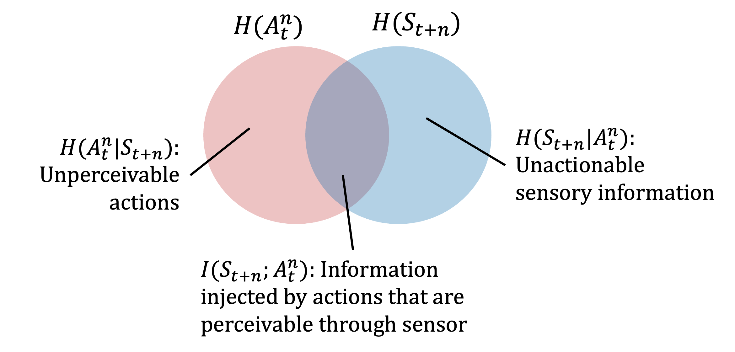
Figure 8: The Venn diagram of mutual information $I(S_{t+n};A^{n}_{t})$. Empowerment is the maximum of this mutual information for a given action channel.

Similar to predictive information, a decomposition of the mutual information in equation (11) is shown in Figure 8. To intuitively understand two conditional entropies, we utilise the box-pushing example presented in [39]: a grid world with a robot that can move anywhere except where the box is. If the box is pushable but the robot’s sensors cannot capture the box’s location, then the robot cannot perceive its box-pushing actions. This is captured in $H(A_{t}^{n}|S_{t+n})$, the unperceivable actions. On the other hand, if the robot can see where the box is but cannot move it, then this information is reflected in $H(S_{t+n}|A_{t}^{n})$, the unactionable sensory information. Only the amount of information that is both actionable and perceivable contributes to empowerment.

In summary, an empowerment-driven agent takes actions that maximise its ability to influence the external world in ways that are perceivable by its own sensors. In multi-agent settings, it has been shown that empowerment-maximisation for individual agents leads to spontaneous coordination among the collective [40, 70, 71]. This coordination arises because shared information enhances an individual’s empowerment, or informally, its ability to make an influence.

Examples of predictive information and empowerment in collective systems, along with their comparisons, are presented in Section VI.

IV.3 Beyond intrinsic motivation

Another prominent approach to derive behaviours based on fundamental principles is the free-energy principle which offers a formal account for the representational capacities of physical systems [46]. The free-energy principle was initially proposed by Friston et al.[45] as an attempt to explain embodied perception-action loops in neuroscience, thus providing an understanding of the dynamics of the brain and decision-making. Adoption of this principle led to wide applications in the study of learning [47, 48, 72], evolutionary dynamics [73], social interactions [74] and collective intelligence [75, 50]. The principle centres on the idea that self-organising biological agents have a natural inclination to resist disorder. It is argued that, as a result, the brain attempts to minimise uncertainty or surprise.

The mechanism derived from the free-energy principle is commonly referred to as active inference. Similar to predictive information and empowerment, active inference can be conceptualised under the perception-action loop representation, although based on different relationships between state variables (Figure 9).

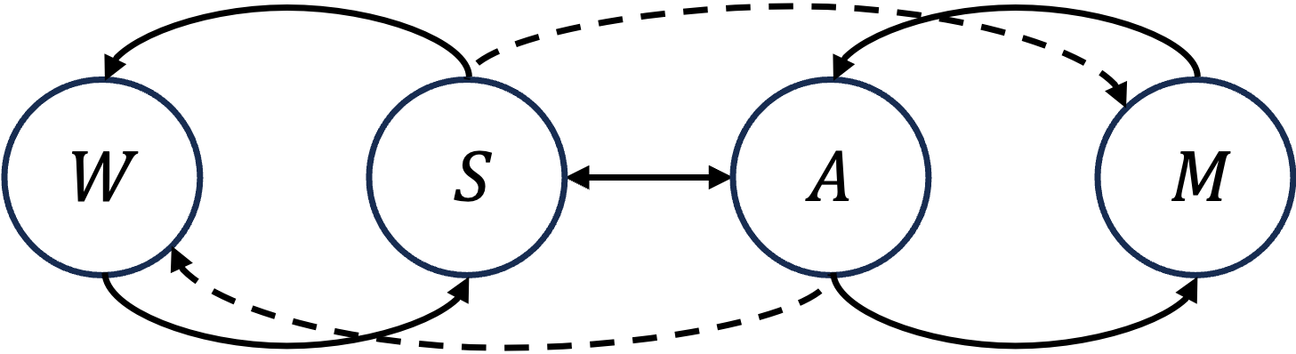
Figure 9: The diagram illustrates interaction between elements in the active inference framework. Solid lines represent influences between components. Dash lines represent directed influence from sensory to internal or from action to external, which correspond to the two stages of active inference. Figure is adapted from [49].

An underlying assumption in active inference is that the brain makes Bayesian inference over the external (world) states. Bayesian inference relies on some prior probability distribution over the unknown world and updates the distribution when more information is available. The main ingredients in the formulation of active inference are the generative model $p$ and the approximate posterior distribution $q$. The generative model $p$ maps causes (external states $W$) to consequences (sensory $S$, action $A$ and internal state $M$). It encodes the dynamics of the external world and integrates the agent’s prior preferences of behaviour [49]. While Bayesian inference relies on updating the prior distribution $p$ to the posterior $p(\cdot|observations)$ given the observed data, the posterior is notoriously costly to compute. To reduce the computational difficulty, a parameterised distribution $q$ is employed as an approximation to the true posterior $p(\cdot|observations)$. The approximation distribution $q$ is parameterised by the internal states $M$, which supplies the sufficient statistics of the conditional distribution. The Bayesian inference process with an approximated posterior distribution is referred to as variational Bayesian inference. It is worth noting that the integration of external goals in the generative model sets active inference apart from the other pure intrinsic motivation approaches.

The variational free energy is defined as the Kullback–Leibler divergence between the approximate posterior distribution $q$ and the generative model $p$. The expression can be expanded in terms of the difference between a term that resembles expected energy and an entropy term, hence the name “free energy”[49]:

$$\begin{split}\mathcal{F}:&=\mathbb{E}_{q}\left[\log\frac{q(w)}{p(s,a,m,w)}\right]\\ &=\underbrace{\mathbb{E}_{q}[-\log p(s,a,m,w)]}_{\text{Expected energy}}-\underbrace{\mathbb{E}_{q}[-\log q(w)]}_{\text{Entropy}}\end{split}$$ (16)

However, the quantity called in this approach “free energy” is different from the thermodynamic free energy. In active inference, it is instead the variational free energy formulated in terms of information theoretic quantities, relating to the Bayesian inference process [45, 49]. Informally, anything that can be represented in the form:

$$\text{free energy}=\text{energy}\pm\text{const.}\times\text{entropy}$$ (17)

can be interpreted as “free energy” [76].

Active inference involves two alternating stages: belief update and action selection. During belief update, the agent optimises the internal representation of the generative model $p$ given the sensory samples; in action selection, the agent’s action ensures that it samples sensory data that aligns with its current representation. The belief update stage addresses uncertainty about the current generative model, while the action selection stage addresses uncertainty about the future (including future hidden states and future observable outcomes) [77, 48].

The active inference approach has been shown to generate collective behaviour in a group of individuals, each driven by the free-energy minimisation scheme [50]. Collective dynamics are influenced by the individual’s belief about uncertainty and can also be tuned to the changing environment by parameter learning over a slower timescale.

Equation (16) can be rearranged in terms of the complexity of the internal model and the accuracy of its representation. In this configuration, minimising free energy is equivalent to reducing complexity, consequently resulting in optimised energy consumption [78, 49]:

$$\begin{split}\mathcal{F}&=\mathbb{E}_{q}[\log q(w)-\log p(w)]-\mathbb{E}_{q}[\log p(s,a,m|w)]\\ &=\underbrace{\text{KL}[q(w)||p(w)]}_{\text{Complexity}}-\underbrace{\mathbb{E}_{q}[\log p(s,a,m|w)]}_{\text{Accuracy}}\end{split}$$ (18)

While equation (18) implies a connection between minimizing free energy and reducing energy cost under Landauer’s principle [78], the relationship is not explicitly formulated as a ratio of informational gain to energetic costs.

A more detailed example of free-energy minimisation and the comparison with other approaches is provided in Section VI.

V Thermodynamic efficiency

At this stage we point out that the three information-theoretic approaches reviewed in the previous section do not explicitly account for the corresponding energy costs. Thermodynamic efficiency, on the other hand, takes into consideration both the benefits and the associated costs of maintaining order within the system. Before presenting a formal definition of thermodynamic efficiency, it is important to differentiate between thermal and thermodynamic efficiency.

V.1 Thermal vs thermodynamic efficiency

Let us consider a system undergoing a non-ideal process in which it receives energy and performs useful work. Not all the received energy is converted into work; some is inevitably lost as heat, which does not contribute to work output (Figure 10). Thermal efficiency measures the system’s efficiency of converting energy to work, and is defined as the ratio of useful work output to total energy input, both measured in joules, rendering it a dimensionless quantity. In a non-ideal process, the second law of thermodynamics implies that this ratio is less than one.

In contrast, thermodynamic efficiency assesses the conversion of work into the system order, measured during a quasi-static change in the underlying control parameter. It pertains to systems involving interactions among multiple components, and considers the benefit of increasing order within a collective system against the thermodynamic cost incurred. A system may transition from a disordered to an ordered state by altering a control parameter according to a specific protocol. Thermodynamic efficiency evaluates how efficiently the system converts the carried out work into order, at each specific value of the control parameter (Figure 11). It is quantified as the ratio of the reduction in the system’s configuration entropy (predictability gain) to the generalised work performed during the control parameter adjustment, expressed in units of bits per joule (subject to the unit of the Boltzmann constant $k_{B}$, e.g., see the expression for entropy, defined in the context of thermodynamics in Equation (21)):

$$\eta(\theta)=\frac{-d\mathbb{S}/d\theta}{d\langle\beta\mathbb{W}_{gen}\rangle/d\theta}$$ (19)

where $\theta$ is the control parameter, $\mathbb{S}$ denotes the configuration entropy of the system, and $\mathbb{W}_{gen}$ denotes the generalised work performed to change the control parameter.

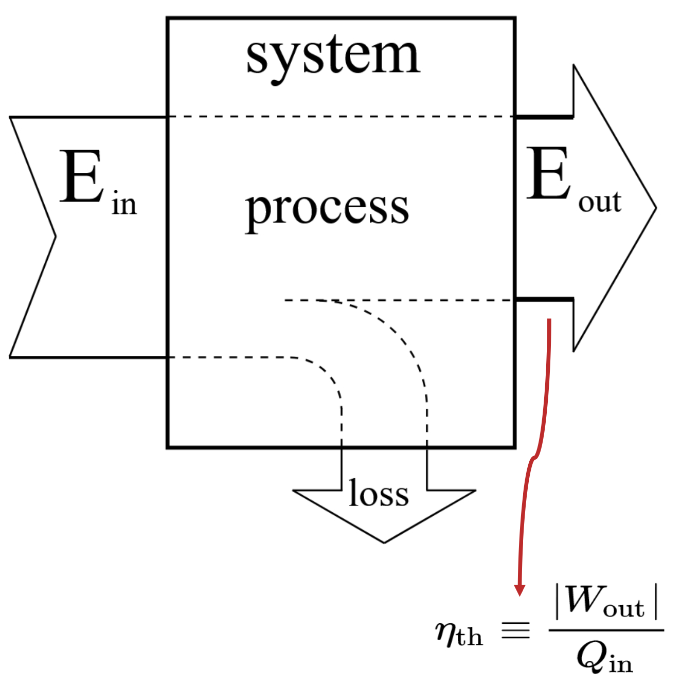
Figure 10: Thermal efficiency for a system undergoing a specific process. It is generally defined as the dimensionless ratio between the total work output and the total energy input. Adapted from [79].

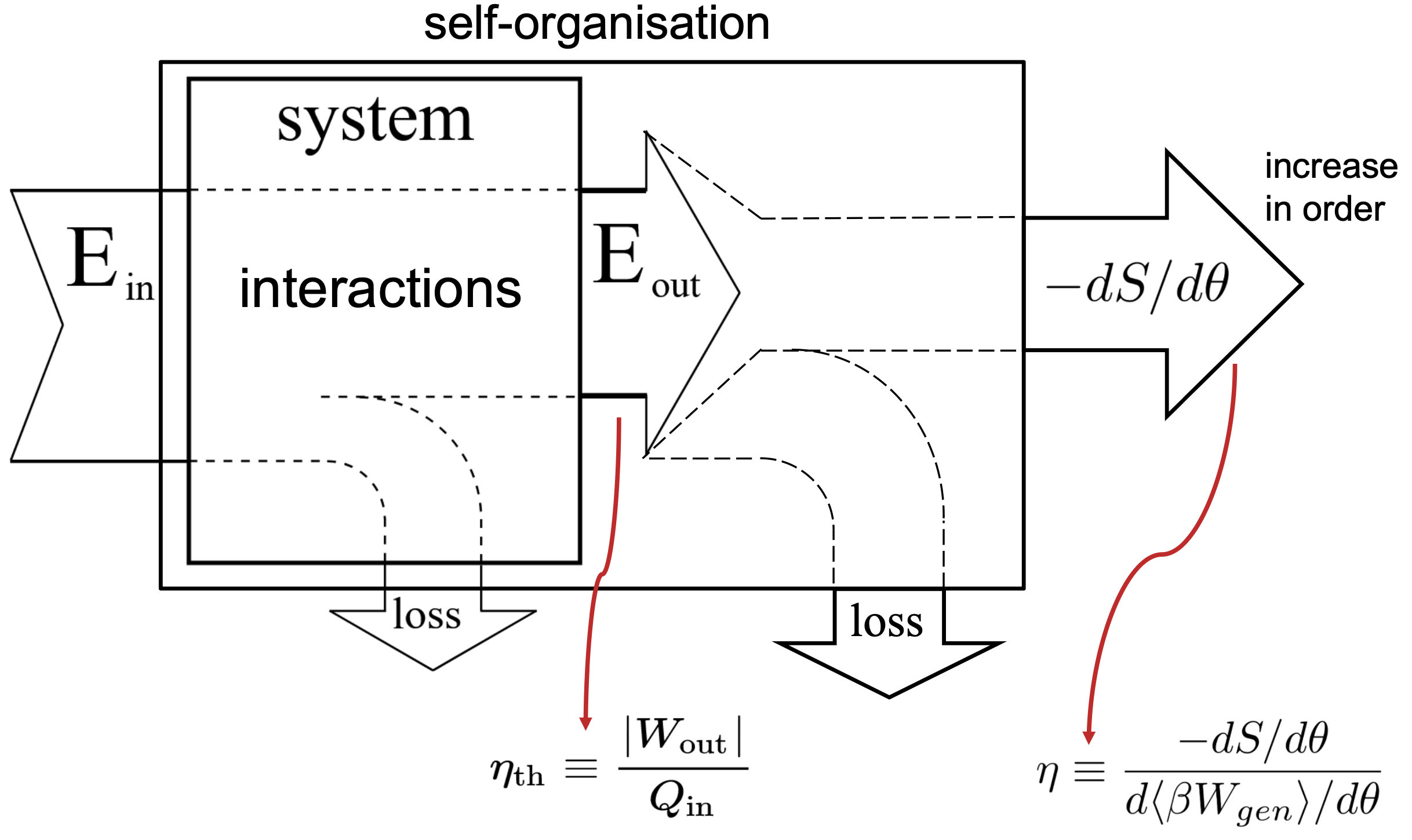
Figure 11: Thermodynamic efficiency for a system. It is defined as the ratio between the increase in order (measured in bits) and change in the generalised work carried out to generate the order (measured in joules). This quantity has a unit of bits per joule.

V.2 Thermodynamic preliminaries

The configuration of a collective system refers to the arrangement of the system’s components, usually the geometric or positional arrangement of the components at a specific moment, for example, the up or down orientations of all the atoms in a ferromagnetic substance. The configuration entropy represents the amount of uncertainty in the system’s arrangement. Lower configuration entropy suggests a limited set of possible configurations, indicating more predictable and coordinated behaviour for the collective system. It is also easier to control or guide the system towards a desired state if there is less uncertainty in the system configurations.

We consider the collective variable $\mathcal{X}_{k}(x)$ defined as a function of the configuration $x$, and the thermodynamic variable $\theta_{k}$ conjugate to $\mathcal{X}_{k}(x)$. A collective variable represents the behaviour of many microscopic components and characterises the macroscopic state of the system resulting from the specific configuration. For example, volume and pressure are a pair of collective and conjugate thermodynamic variables. The probability of the system being in configuration $x$ can be expressed by the Gibbs measure [80, 81]:

$$p(x;\vec{\theta})=\frac{1}{Z(\vec{\theta})}e^{-\sum_{k}\theta_{k}\mathcal{X}_{k}(x)}$$ (20)

where $Z(\vec{\theta})$ is the partition function that normalises this probability over all configurations. For simplicity, we consider single-parameter $\theta$ for the rest of the discussion, but the same framework applies to multi-parameter cases.

In thermodynamic context, the configuration entropy of the system given by the Gibbs ensemble is defined as:

$$\mathbb{S}(\theta)=-k_{B}\sum_{x}{p(x;\theta)\log p(x;\theta)}$$ (21)

and can be converted to the Shannon entropy $H_{X}=-\sum_{x}p(x)\log p(x)$ by dividing by a factor of $k_{B}$.

The order parameter $\phi$ conjugate to the thermodynamic variable $\theta$ is related to the expected value of the corresponding collective variable $\mathcal{X}$:

$$\phi=-k_{B}T\langle\mathcal{X}\rangle$$ (22)

The Gibbs free energy $\mathbb{G}$ is defined as:

$$\mathbb{G}=\mathbb{U}-T\mathbb{S}-\theta\phi$$ (23)

where $\mathbb{U}$ is internal energy.

Evaluating the work done to or extracted from the system requires the specification of a protocol in which the control parameter varies. Henceforth, we consider a quasi-static protocol, which means that the change of control parameter occurs infinitely slowly so that the system remains in thermal equilibrium with its surroundings at all times. The generalised first law of thermodynamics relates the generalised internal energy $\langle\mathbb{U}_{gen}\rangle=\mathbb{U}-\theta\phi$ in the sense of Jaynes [82], the generalised heat flow (from the environment to the system) $\langle\mathbb{Q}_{gen}\rangle$, and the generalised work $\langle\mathbb{W}_{gen}\rangle$:

$$\Delta\langle\mathbb{U}_{gen}\rangle=\Delta\langle\mathbb{Q}_{gen}\rangle+\Delta\langle\mathbb{W}_{gen}\rangle$$ (24)

Since a change in the configuration entropy is matched by the heat flow ($\Delta\mathbb{Q}_{gen}=T\Delta\mathbb{S}$), the thermodynamic work equals the change in free energy, that is, $\Delta\langle\mathbb{W}_{gen}\rangle=\Delta\mathbb{G}$ (the complete argument is presented in Ref. [52]). Taking the first derivative with respect to control parameter $\theta$ yields:

$$\frac{d\langle\mathbb{W}_{gen}\rangle}{d\theta}=\frac{d\mathbb{G}}{d\theta}$$ (25)

V.3 Fisher information

At this stage we turn our attention to the Fisher Information which is related to Gibbs free energy. The Fisher information measures the amount of information that an observable random variable carries about an unknown parameter $\theta$ which may be influencing the probability of observations. In order words, Fisher information quantifies the sensitivity of observations to the change of parameter $\theta$. Mathematically, Fisher information is defined as the variance of the score function, where the score is the derivative of the log-likelihood function with respect to $\theta$ [61]:

$$\begin{split}\mathbb{I}(\theta)&=E\left[\left(\frac{\partial}{\partial\theta}\log p(x;\theta)\right)^{2}\right]\\ &=\int_{x}\left(\frac{\partial}{\partial\theta}\log p(x;\theta)\right)^{2}p(x;\theta)dx\end{split}$$ (26)

It has been established that Fisher information is proportional to the rate of change of the order parameter with respect to the change in control parameter, being analogous to susceptibility [81] (compare with equation (1)):

$$\mathbb{I}(\theta)=\beta\frac{d\phi}{d\theta}\ \propto\ |\theta-\theta_{c}|^{-\gamma}$$ (27)

In explaining the relationship between Fisher information and thermodynamic efficiency, we point out that Fisher information is proportional to the second derivative of Gibbs free energy [80, 83, 84, 85]:

$$\mathbb{I}(\theta)=-\beta\frac{d^{2}\mathbb{G}}{d\theta^{2}}$$ (28)

As established in [52] under a quasi-static protocol, following the first law of thermodynamics, equations (25) and (28) yield:

$$\frac{d\langle\beta\mathbb{W}_{gen}\rangle}{d\theta}=\int_{\theta}^{\theta^{*}}{\mathbb{I}(\theta^{\prime})}d\theta^{\prime}$$ (29)

where the integral is computed from the point of evaluation $\theta$ to the “zero-response point” $\theta^{*}$ defined as the point where a perturbation of control parameter $\theta$ extracts no work from the system.

V.4 Perspectives on thermodynamic efficiency

Using results of the preceding subsections, the thermodynamic efficiency of interactions can be expressed in two different ways [52, 54]:

$$\eta(\theta)=\underbrace{\frac{-d\mathbb{S}/d\theta}{d\langle\beta\mathbb{W}_{gen}\rangle/d\theta}}_{\text{In thermodynamic terms}}\\ =\underbrace{\frac{-d\mathbb{S}/d\theta}{\int_{\theta}^{\theta^{*}}{\mathbb{I}(\theta^{\prime})}d\theta^{\prime}}}_{\text{In computational terms}}$$ (30)

Thermodynamic efficiency offers a dual perspective on the energy dynamics within systems, encompassing both thermodynamic and computational dimensions. From the thermodynamic viewpoint, this quantity captures the gain in internal order within a collective system of interacting agents (e.g., a swarm) relative to the overall work required to adjust the agent interactions. From a computational viewpoint, thermodynamic efficiency measures the increase in predictability (reduction of uncertainty) of collective action gained by accumulating additional sensitivity to changes in the control parameter along the path $\theta\rightarrow\theta^{*}$. For example, a swarm may gain predictability of a collective response by adjusting the individual’s alignment strength or the number of effective neighbours influencing an individual. This, however, may come at the expense of additional sensitivity to changes in these parameters, so that coherent motion may be disrupted by a change of alignment strength or a reduced number of effective neighbours.

The thermodynamic efficiency was shown to peak at the critical regime in complex systems. Some recent studies have pursued this direction, albeit in different application settings. Crosato et al. [52] explored this relationship near criticality using a model of self-propelled particles. They defined thermodynamic efficiency $\eta$ as the reduction in entropy relative to the work done on the system and demonstrated that as particles undergo a kinetic phase transition from disordered to coherent motion, $\eta$ peaks at the critical regime.

This concept was also applied for urban transformations [51], where the maximum entropy principle coupled with Lotka-Volterra dynamics was used to study shifts in population and income distribution in urban areas. The study considered the thermodynamic efficiency $\eta$ expressed as the increase in predictability of the population income flows relative to the thermodynamic work required to adjust the social disposition. The study underscored a phase transition between monocentric and polycentric urban configuration induced by quasi-static changes in the underlying social disposition parameter. Importantly, the thermodynamic efficiency was observed to peak at the phase transition.

In the context of epidemic modelling, Harding et al. [53] examined the thermodynamic efficiency $\eta$ of contagions diffusing on a network, defining $\eta$ as the ratio of uncertainty reduction in the system to work expenditure required to quasi-statically change the control parameter (e.g. the infection transmission rate). Their numerical analyses identified a phase transition between sub-critical (non-epidemic) and super-critical phases (epidemic) as the infection transmission rate increased, with the highest thermodynamic efficiency observed at the critical regime.

A later study by Nigmatullin et al. [54] derived an analytical expression for the thermodynamic efficiency of interactions in the canonical Curie-Weiss model, showing that it diverges at the critical point of second-order phase transitions as $\theta\rightarrow\theta_{c}$:

$$\eta(\theta)=\begin{cases}-\frac{\theta_{c}}{2k_{B}}(\theta-\theta_{c})^{-1}&\text{for }\theta<\theta_{c}\\ \frac{1}{k_{B}}(\theta-\theta_{c})^{-1}&\text{for }\theta>\theta_{c}\end{cases}$$ (31)

where $\theta$ is the temperature, that is:

$$\eta(\theta)\propto|\theta-\theta_{c}|^{-1}\ .$$ (32)

In general, the gained predictability enhances coordination within the system, facilitating efficient interactions. Systems with high or maximal thermodynamic efficiency tend to operate at or near the critical regime where long-range correlations and scale invariance bring collective benefits. Thus, thermodynamic efficiency may provide an intrinsic utility to the system, explaining the ubiquity of collective animal behaviours, such as swarming, herding, flocking, and so on, which balance energy costs with group coherence.

VI An example

In previous sections, we explored different approaches to quantifying the intrinsic utility of collective behaviour. In this section, we compare the four considered approaches — predictive information, empowerment, active inference, and thermodynamic efficiency — using the canonical Ising model as a common example.

VI.1 The 2D Ising model

The 2D Ising model offers a simplified representation of ferromagnetism in statistical mechanics. It models a collection of sites that can each exhibit either an up-spin or down-spin configuration, while interacting with their neighbours to create a complex aggregate dynamic. The 2D Ising model is particularly relevant to our comparison due to its characteristic phase transition in the collective dynamics.

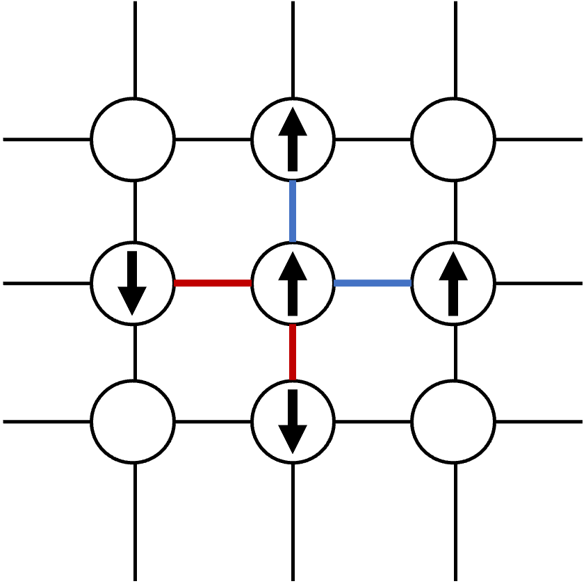
Figure 12: A lattice of atoms with dipole magnetic moments. Links in red represent higher energy bonds (where two adjacent atoms have opposite spins), and blue represents lower energy bonds (where two adjacent atoms are aligned).

The 2D-Ising model considers a lattice of atoms with magnetic spins oriented either up or down (Figure 12). The vertices of the lattice are referred to as “sites” and the edges as “links”. Assuming the absence of an external magnetic field, the energy of a site is determined by the total energies in the links with its neighbours. Each site prefers to be in a lower energy state. For ferromagnetic materials maintaining a link between two sites with opposite spins requires additional energy, hence there is a natural tendency for a site to align its spin with those of its neighbours. The susceptibility of a site to neighbouring influences depends on the coupling parameter $J$. A high value of $J$ indicates strong coupling between sites, leading to a greater tendency for spins to align with neighbouring sites.

In this example, the dynamics of the Ising model is interpreted from a perception-action loop perspective: each site acts as an agent that senses the energy of its neighbourhood and “decides” whether to flip its spin or maintain its current state. The agency of each site is determined by the choice of the coupling parameter $J$. With a high $J$ value a site is more prone to align with its neighbours, and vice versa. This parameter governs the strength of the site’s response to the neighbourhood’s energy landscape, influencing its decision to align with neighbouring spins.

To draw a clearer connection between the Ising model and the perception-action loop, we consider that each of the four elements of the perception-action loop has a corresponding representation in the Ising model:

• $W$ (world): the magnetisation (average spin) of the lattice;

• $S$ (sensory): the energy state of a site (defined in eq. (33));

• $A$ (action): flipping of the spin or remain unchanged, with flip = $-1$ and no-flip = $+1$;

To quantify the energy, we define:

• $N$: the number of sites in the lattice;

• $J$: the coupling strength between adjacent sites;

• $\sigma^{(i)}$: the spin of site $i$, with $+1$ representing up spin and $-1$ is down;

• $\underline{\sigma}$: the configuration of the lattice $\underline{\sigma}=\{\sigma^{(1)},\sigma^{(2)},...,\sigma^{(N)}\}$.

Let $i$,$j$ be two sites connected by a link, then:

$$\sigma^{(i)}\sigma^{(j)}=\begin{cases}+1&\text{if sites i, j aligned}\\ -1&\text{if sites i, j misaligned}\end{cases}$$

Considering the interactions between a site and its nearest four neighbours only, the total energy of this site is:

$$E^{(i)}=\sum_{j\in\nu^{(i)}}{-J\sigma^{(i)}\sigma^{(j)}}$$ (33)

where $\nu^{(i)}$ denotes the set of neighbouring sites of $i$.

We simulate the process using the Metropolis algorithm [86, 87]. Each time, a site in the lattice is chosen randomly. The Metropolis algorithm assumes the following probability for a flipping action:

$$p(\text{flip})=\begin{cases}1&\text{if }dE^{(i)}\leq 0\\ e^{-\beta dE^{(i)}}&\text{if }dE^{(i)}>0\end{cases}$$ (34)

where $\beta$ is the inverse of temperature and $dE^{(i)}$ is the change in energy after a flip. We assume $\beta=1$ for the purpose of this experiment. The energy change $dE^{(i)}$ is computed as:

$$\begin{split}dE^{(i)}&=E^{(i)}(\text{after flip})-E^{(i)}(\text{before flip})\\ &=\sum_{j\in\nu^{(i)}}2J\sigma^{(i)}\sigma^{(j)}\end{split}$$ (35)

Equation (34) implies that a site will always flip its spin ($p(\text{flip})=1$) if doing so results in a lower energy state. However, if the flip leads to a higher energy state, which means that the site goes from aligning to misaligning with its neighbouring sites, the coupling strength $J$ determines the site flipping likelihood. All else being equal, a higher value of $J$ results in a lower probability of flipping or higher likelihood to remain aligned with neighbouring sites.

The experimental setup is detailed in Appendix A, and the source code is available in [58]. For each intrinsic utility approach, we plot the measure against the coupling strength $J$ and identify the value of $J$ that optimises the utility. We then discuss the implications of these different optimal ranges and the associated characteristics of self-organised behaviours.

VI.2 Computational results

In this experiment, we hold the coupling parameter $J$ constant and run the simulation until the system reaches equilibrium. We then calculate the corresponding predictive information, empowerment, free energy (active inference), and thermodynamic efficiency. To eliminate the effects of initial conditions, we average these quantities across multiple simulations for each $J$. This process is repeated for a range of $J$ values. We aim to identify the optimal range of $J$ values under each approach in order to answer the question: “If the coupling strength $J$ evolves independently using each of these quantities as the fitness function, what behaviour should we expect when fitness is optimised?”

We collect the following data for the selected site and the lattice at time $t$:

• $a_{t}$: the action of flip (-1) or no-flip (+1) at time $t$;

• $\sigma_{t},\sigma_{t+1}$: spin of the selected site before and after the action is performed;

• $w_{t},w_{t+1}$: the magnetisation of the lattice before and after the action is performed;

• $s_{t},s_{t+1}$: the selected site’s sensory state before and after the action is performed;

The data form time series $\{a_{t}\}$, $\{\sigma_{t}\}$, $\{\sigma_{t+1}\}$, $\{w_{t}\}$, $\{w_{t+1}\}$, $\{s_{t}\}$, $\{s_{t+1}\}$, using which we compute the intrinsic utility measures. Leveraging the homogeneity of the lattice sites, we can aggregate the random samples from different sites to compute the measures. This approach ensures that the results represent the intrinsic utility values corresponding to the coupling strength $J$ as experienced by an average site within the lattice.

VI.2.1 Predictive information

For a given coupling strength $J$, the corresponding one-step predictive information is the mutual information between the pre-action sensory state and the post-action sensory state:

$$\begin{split}\mathcal{I}&=I(S_{t+1};S_{t})\text{ [bits]}\\ &=\sum_{s_{t}}\sum_{s_{t+1}}p(s_{t},s_{t+1})\log\frac{p(s_{t},s_{t+1})}{p(s_{t})p(s_{t+1})}\end{split}$$ (36)

where the probability distributions are parameterised by $J$.

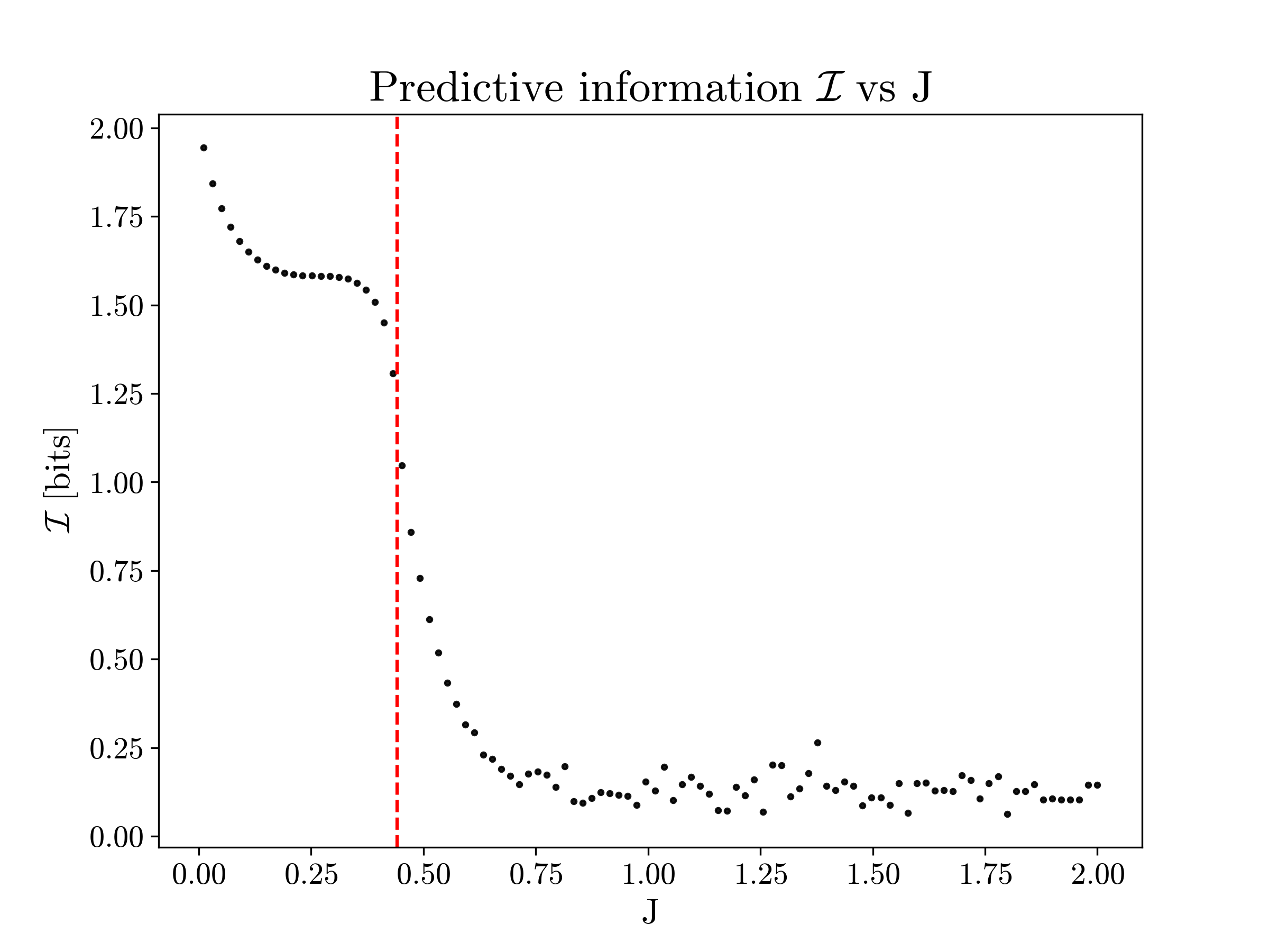
Figure 13: Average predictive information plotted against different values of $J$, computed from 20 simulations, each of 20 million time steps on a $50\times 50$ square lattice with periodic boundary conditions. Predictive information maximises when $J$ is small (weak coupling), and the average site exhibits explorative behaviour.

Figure 13 shows predictive information $\mathcal{I}$ for each coupling strength $J$. Predictive information is maximised when $J$ is low, suggesting that a system driven by predictive information would evolve into a highly exploratory state characterised by weak coupling between the sites. Given equation (8), predictive information can be decomposed into two terms:

$$I(S_{t+1};S_{t})=H(S_{t+1})-H(S_{t+1}|S_{t})$$ (37)

where the entropy $H(S_{t+1})$ represents the richness of future sensory states and the conditional entropy $H(S_{t+1}|S_{t})$ represents unpredictability.

In this example, sensory state $S$, which is the energy of a site, changes from $s$ to $-s$ if the site flips its spin. The trend observed in Figure 13 can be understood by examining the entropy and conditional entropy terms under two extreme scenarios of $J$:

• When $J\rightarrow 0$: The weak coupling leads to frequent flipping of the sites, resulting in a sequence of alternating sensory states. Consequently, $H(S_{t+1})$ is high due to the constant activity, and $H(S_{t+1}|S_{t})=0$ because $S_{t+1}=-S_{t}$ when sites flip indefinitely. Thus, the predictive information is high, reflecting a combination of rich sensory diversity and yet fully predictable future states for a local site;

• When $J\rightarrow+\infty$: The strong coupling prevents sites from flipping, leading to static sensory states. In this scenario,$H(S_{t+1}|S_{t})=0$ because $S_{t+1}=S_{t}$ if the site never flips, and $H(S_{t+1})\rightarrow 0$ as all sites align uniformly. Therefore, predictive information is low, indicating a predictable and homogeneous system with little sensory diversity.

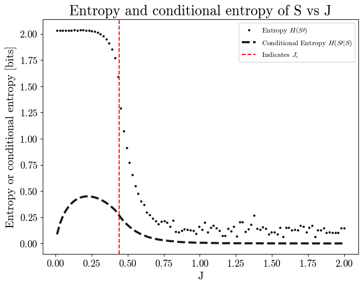
Figure 14: Decomposition of predictive information into richness (dotted line) and unpredictability (dash line) components; predictive information is the difference between the two terms. Results obtained from the average over 20 simulations, each of 20 million time steps on a $50\times 50$ square lattice with periodic boundary conditions.

We further note the inflexion point in Figure 13 just before the point $J_{c}=\frac{1}{2}\ln(1+\sqrt{2})\approx 0.4407$ which corresponds to the critical value for the canonical 2D-Ising model. As shown in Figure 14, $H(S_{t+1}|S_{t})$ first increases with $J$ and then decreases after the critical region, while $H(S_{t+1})$ continues to decrease, creating the inflexion point in the predictive information plot.

VI.2.2 Empowerment

To compute the average empowerment of a site at equilibrium, we first analytically derive the channel capacity of the action channel. In this model, the action channel is defined by the conditional probability $p(s_{t+1}|a_{t})$. The state of pre-action sensory $s_{t}$ determines this conditional probability, and thus, two cases must be considered separately: $p(s_{t+1}|a_{t},s_{t}\neq 0)$ and $p(s_{t+1}|a_{t},s_{t}=0)$.

When $s_{t}\neq 0$, meaning that the up and down spins of the neighbours are not perfectly balanced, a flipping action will result in the next sensory state becoming the opposite of what it was before the flip. The action channel, in this case, resembles the one shown in Figure 15. This is a noiseless binary channel and, by definition, has channel capacity $C(s_{t})=1$ bit. Full capacity is achieved when the site follows action distribution $p(a)=(\frac{1}{2},\frac{1}{2})$.

Figure 15: A noiseless binary channel. Channel capacity C = 1 bit.

If $s_{t}=0$, the channel simply reduces to the one shown in Figure 16, that is, a channel that carries no information as the output is always the same. This means that the channel capacity is zero, $C(s_{t})=0$ bit.

Figure 16: A single output channel. Channel capacity C = 0 bit.

Combining these two cases, we obtain:

$$C(s_{t})=\begin{cases}1&\text{if }s_{t}\neq 0\\ 0&\text{if }s_{t}=0\end{cases}$$ (38)

The average one-step empowerment, averaged over the distribution of channels, is computed as follows:

$$\mathfrak{\bar{E}}=\sum_{s_{t}}{p(s_{t})C(s_{t})}\text{ [bits]}$$ (39)

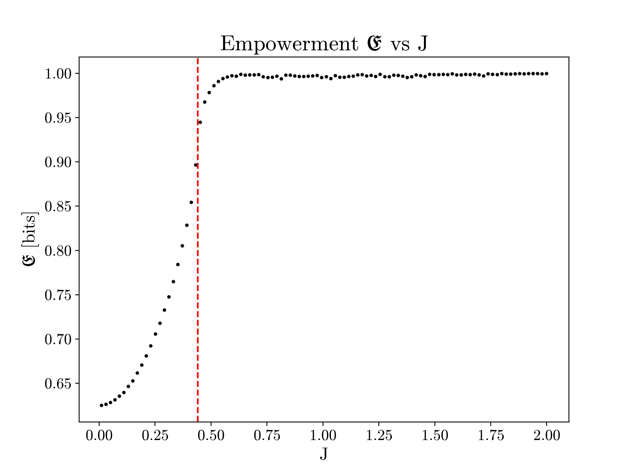
Figure 17: Average empowerment plotted against different values of $J$, computed from 20 simulations, each of 20 million time steps on a $50\times 50$ square lattice with periodic boundary conditions. Empowerment optimises when $J$ is large (strong coupling), and the collective exhibits a stable structure. Such structure in positional configuration increases an average site’s ability to perceive the impact of its action on the environment.

Based on empowerment, the resulting optimal $J$ is at the higher end of the spectrum (Figure 17), where the lattice exhibits a more stable structure with most of the atoms aligned. Empowerment measures an agent’s ability to inject information into the environment via current actions and later retrieve the information via its sensors. A site’s action is most perceivable when all its neighbours align in the same direction, in which case the action of flip or no-flip leads to distinct sensory outputs ($s$ or $-s$, $s\neq 0$). Conversely, if four neighbours have an equal split between up and down spins, flipping the spin of a site does not change its sensory state. That is, the site will not be able to perceive the impact of its action. A large positive $J$ value increases the probability of an average site being at the configuration where all its neighbours have the same spin, thereby maximising the site’s empowerment by ensuring its actions produce noticeable changes to its future sensory inputs.

VI.2.3 Variational free energy (active inference)

For the purpose of this study, the active inference framework is adopted from [88], thus focusing solely on its intrinsic component. A negative sign is placed before the expression, effectively transforming the minimisation problem into one of maximising the action value $-\mathcal{F}$. For each possible action $a_{t}\in\{-1\>(\textit{flip}),+1\>(\textit{no-flip})\}$, we compute the one-step negative free energy following the derivation from [88]:

$$\begin{split}-\mathcal{F}{(a_{t})}&=-H(S_{t+1}|W_{t+1},a_{t})\\ &=\sum_{s_{t+1}}\sum_{w_{t+1}}p(s_{t+1},w_{t+1}|a_{t})\log p(s_{t+1}|w_{t+1},a_{t})\end{split}$$ (40)

where the probability distribution is parameterised by coupling strength $J$.

The conditional entropy describes the expected discrepancy between the agent’s (the site’s) perception of the world (the entire lattice) and the actual future state of the world after performing action $a_{t}$. This expectation is computed based on its current internal model $m(\cdot)$. In this context, the agent’s internal model is the empirical conditional distribution of joint random variables ($S_{t+1}$, $W_{t+1}$), conditional on the values of actions $\{a_{t}\}$. It is constructed using time series $\{s_{t+1}\}$, $\{w_{t+1}\}$ and $\{a_{t}\}$.

The non-zero conditional entropy is the result of the agent’s limited sensory information, which only extends to its nearest neighbours, leading to a mismatch between the agent’s view of the world and the actual world. Under active inference, the agent would choose actions (flipping or not) to minimise this discrepancy. However, in the Ising model setting, the site can only adjust its sensitivity (coupling parameter $J$) to the influence of its neighbours. The coupling parameter effectively decides each site’s propensity to flip its spin. This parameter adjustment serves as a proxy for choosing the optimal action to reduce the conditional entropy.

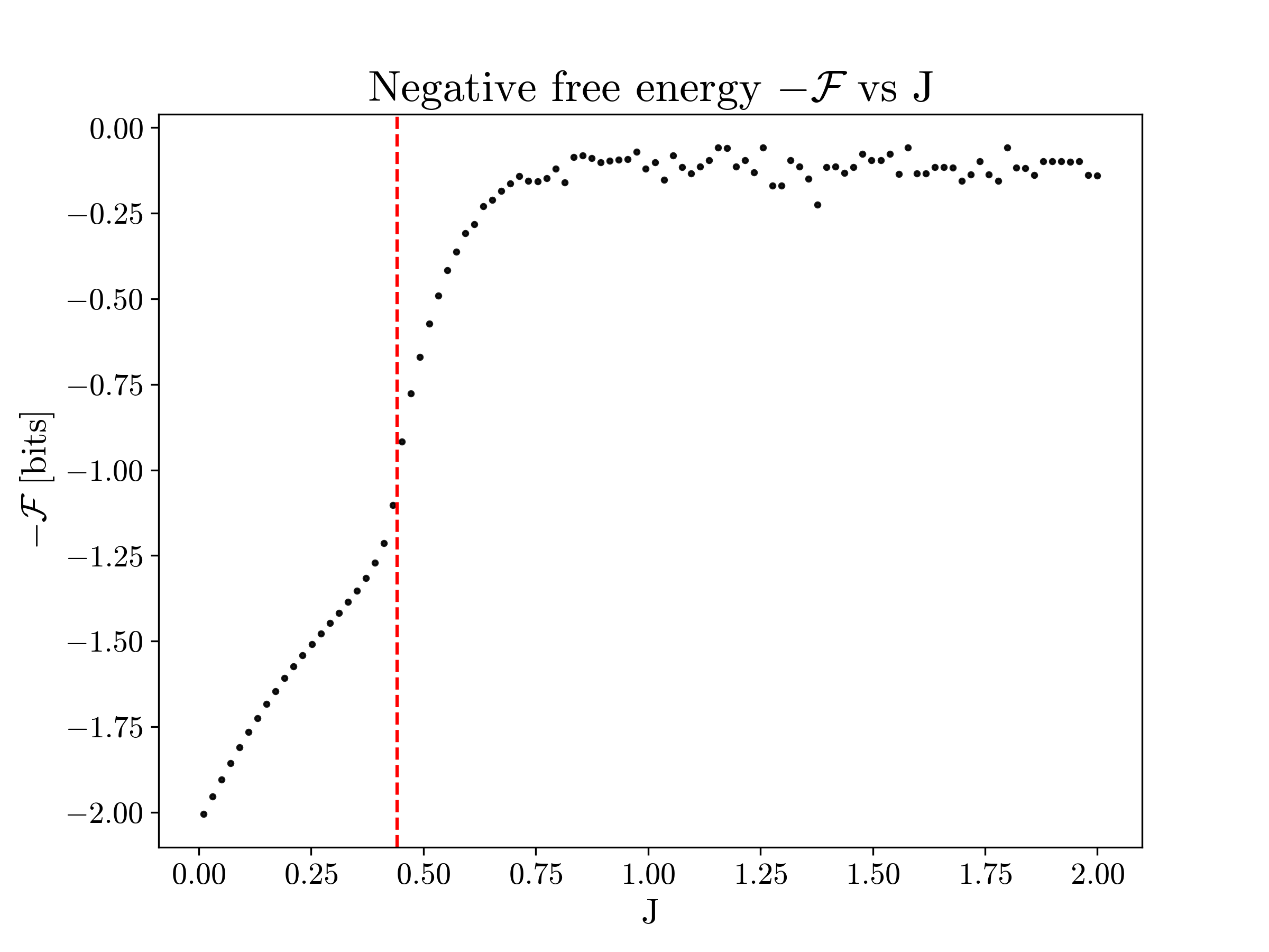
Figure 18: Average negative free energy plotted against different values of $J$, computed from 20 simulations, each of 20 million time steps on a $50\times 50$ square lattice with periodic boundary conditions. Negative free energy maximises when $J$ is large (strong coupling), where the spins are aligned at equilibrium, and the agent (a site)’s approximation of the world state distribution (based on local sensory states) closely matches the actual distribution that generates the world states (global property).

The average negative free energy at equilibrium is computed by weighted average across the proportion of $a_{t}=-1$ (flip) and $a_{t}=1$ (no-flip) actions:

$$-\mathcal{\bar{F}}=-\sum_{a_{t}}{p(a_{t})\mathcal{F}{(a_{t})}}\text{ [bits]}$$ (41)

This measure represents, on average, if a site acts with coupling parameter $J=j$, how much discrepancy it should expect between its internal model (which is based on the local sensory history) and the external world described by the lattice magnetisation. This quantity assesses how well the site’s perception aligns with the underlying global situation.

The negative free energy plot (Figure 18) reveals a similar optimal region for $J$ as the one produced by empowerment. Its negative value reflects how accurately the site’s model of the world (constructed using local information) represents the actual state of global magnetisation. When $J$ is large, more atoms are aligned, increasing the likelihood that an average site correctly perceives the overall spin direction. This alignment results in a higher action value within this range of $J$.

VI.2.4 Thermodynamic efficiency

Thermodynamic efficiency $\eta$ for each corresponding $J$ is computed as:

$$\eta=-\frac{d\mathbb{S}(J)/dJ}{\int_{J}^{J^{*}}{\mathbb{I}(J^{\prime})}dJ^{\prime}}\text{[bits/joule]}$$ (42)

The numerator is the derivative of the configuration entropy $\mathbb{S}$ of the lattice with respect to the control parameter $J$. It represents the reduction of uncertainty in the lattice’s configuration as a result of a small variation in the coupling strength $J$. Using the Kikuchi approximation, the configuration entropy is [89, 90]:

$$\mathbb{S}=\mathbb{S}_{4}-2\mathbb{S}_{2}+\mathbb{S}_{1}$$ (43)

where $\mathbb{S}_{k}$ is the entropy of size k sub-lattices.

The denominator in this calculation is the integral of Fisher information with respect to the control parameter $J$, representing the work required by the system to instigate the change $\delta J$. The integration limit extends from $J$, the point of evaluation, to $J^{*}$, the zero-response point. Ideally, $J^{*}=\infty$, but in this numerical experiment, setting $J^{*}=10$ is sufficient, ensuring that the system reaches perfect order at equilibrium and no further work can be done. The method for numerically computing Fisher information is detailed in Appendix B.

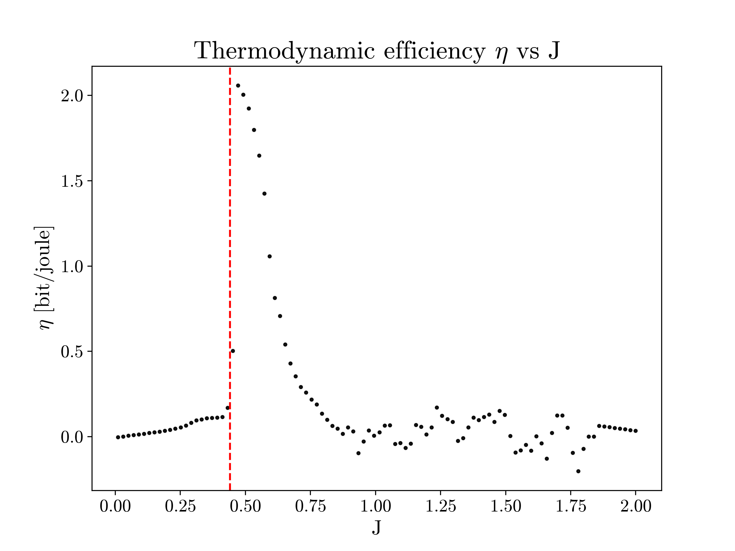
Figure 19: Average thermodynamic efficiency plotted against different values of $J$, computed from 20 simulations, each of 20 million time steps on a $50\times 50$ square lattice with periodic boundary conditions. Efficiency optimises near the critical regime, where a significant portion of the work expended in tuning the parameter $J$ contributes to creating order within the system, that is, small changes of $J$ result in a large decrease in the system’s configuration entropy.

Thermodynamic efficiency reaches optimum when $J$ is near the critical value $J_{c}\approx 0.4407$, as shown in Figure 19. In this range, even a small increase in the control parameter $J$ results in a significant reduction in the system’s disorder. Consequently, the work performed to establish order in the system achieves the highest efficiency. This observation indicates that the collective systems that optimise thermodynamic efficiency at the same time operate at the critical regime.

It is important to note that the numerical values of thermodynamic efficiency tend to exhibit more noise than other metrics. This is due to the computation of the entropy derivative and Fisher information. Despite these numerical nuances, the presented computational results (coupled with prior analytical derivations [54]) suggest that optimising thermodynamic efficiency within a collective system is achieved at the critical regime. This argument frames the thermodynamic efficiency as an intrinsic utility, and provides an explanation why collective behaviours induced by this utility often exhibit critical phenomena.

VII Principle of Super-efficiency

Many natural systems with a large number of interacting components exhibit self-organisation, forming larger structures or coherent collective behaviours without external coordination. Locally interacting neurons collectively perform complex brain functions while processing diverse stimuli [7, 10]. Active matter comprising self-catalytic colloidal particles produces polar collective motion [91, 92]. Starlings form flocks that move in intricate patterns in response to environmental changes [11, 93]. These self-organising collective behaviours are often observed at critical regimes which seem to balance the fluidity (or adaptability) offered by amorphous, disordered groups (e.g., granular materials or liquids) and the stability (or persistence) provided by rigid, ordered structures (e.g., crystalline materials).

The ubiquity of collective behaviours that tend to self-organise near or at critical regimes suggests that there is an underlying principle governing such behaviour across different systems. By abstracting from the specific details of each system, we may uncover not only why collective systems self-organise, but also why self-organisation often brings the collective close to the critical regime. A possible underlying principle would need to interpret these behaviours in terms of generic intrinsic utilities rather than via the typically observed critical phenomena, such as scale invariance and the divergence of correlation length.

We argue that several previous studies of thermodynamic efficiency [51, 52, 53, 54], as well as the computational experiment presented in Section VI, exemplify a general principle of super-efficiency: the efficiency of interactions within self-organising collective systems is maximal at critical points in their dynamics.

The principle of super-efficiency suggests that self-organising collective systems strive to maximise the thermodynamic efficiency of interactions, that is, the ratio between the reduction in configuration entropy and the incurred generalised work (equation (30)). Given a protocol adjusting the interactions among the constituent components of the system, maximisation of the thermodynamic efficiency occurs through tuning the corresponding control parameter:

$$\begin{split}\theta^{*}&=\underset{\theta}{\arg\max}\>\{\eta(\theta)\}\\ &=\underset{\theta}{\arg\max}\>\frac{-\partial\mathbb{S}/\partial\theta}{\partial\langle\beta\mathbb{W}_{gen}\rangle/\partial\theta}\end{split}$$ (44)

In other words, the principle of super-efficiency aims to explain why it is beneficial for a group of interacting agents to operate at the critical regime, rather than how the system could self-organise to this point — the latter question is pursued by SOC models. The underlying rationale is that for a self-organising system with many interacting components, being energetically efficient in reducing disorder and creating internal coordination is advantageous. When the thermodynamic efficiency, considered as an intrinsic utility or a fitness function, attains its maximal value, the system can be interpreted to be super-efficient. In the considered examples the super-efficiency of collective behaviour has occurred at the critical regime, further connecting collective behaviours and critical phenomena.

To re-iterate, a super-efficient self-organising system approaches the point where it can gain maximal predictability of its collective behaviour, given the amount of work available to change the control parameter. Alternatively, given a desired predictability gain, a super-efficient system seeks the point where the energy cost of changing the control parameter is minimal. The considered examples demonstrated that super-efficiency is attained at the critical points.

VIII Conclusion

This paper explored the intrinsic utility for self-organising collective systems to operate at the critical regime. We have discussed various information theoretic approaches as well as an approach that combines information theory and thermodynamics as candidates for understanding the “usefulness” of a dynamical system to operate at the critical point. An experiment was designed connecting the canonical 2D Ising model to the perception-action loop, enabling a comparison of various intrinsic utility approaches within a single example. The optimal coupling strength $J$ was computed for different approaches, including predictive information maximisation, empowerment maximisation, free energy minimisation, and thermodynamic efficiency maximisation. Each approach exhibited a distinct optimal range of parameter values, offering intuitive insights into the underlying driver shaping collective behaviour:

• Predictive information maximises at low coupling strength, balancing sensory richness with predictability;

• Empowerment maximises at high coupling strength, where the individuals have maximal influence over the environment;

• Free energy minimisation (with intrinsic component only) also leads to high coupling strength, where local observations align most closely with the global configuration;

• Thermodynamic efficiency maximisation optimises near the critical regime, achieving maximum entropy reduction per unit of work expended.

Thus, thermodynamic efficiency, measured by the entropy reduction or predictability gain relative to the associated thermodynamic work carried out, might be a candidate for the intrinsic utility of criticality.

Informed by this analysis, as well as the relevant studies of thermodynamic efficiency [52, 51, 53, 54], we proposed a general principle, the principle of super-efficiency, that may explain why collective systems self-organises to the critical point. The principle of super-efficiency states that at the critical point, a self-organising system achieves an optimal entropy reduction relative to the thermodynamic costs. The ability to reduce entropy efficiently grants the collective system an advantage, offering an intrinsic motivation to operate near the critical point. We believe that the principle of super-efficiency has implications for the broader field of guided self-organisation, informing the design of intelligent, adaptive systems that achieve superior coordination, decision-making, and resource management.

Appendix A Simulation of Ising model

The following settings have been applied to the simulations:

• Lattice: a torus-shape lattice of size 50$\times$50;

• Coupling strength $J$: values taken from range (0,2) with increments $\delta J$ = 0.02;

• Number of simulations: 20 simulations with different random seeds are run for each value of $J$;

• Number of time steps: for each simulation, 20 million steps are simulated;

• Number of samples (for predictive information, empowerment and variational free energy): in each simulation, the last 200k steps are sampled to compute the corresponding information-theoretic quantities. The quantities are then averaged over 20 simulations;

• Number of samples (for thermodynamic efficiency): in each simulation, configuration distributions are sampled from the last 200k time steps with a sub-sampling interval of 2,500 time steps (1 sweep of the lattice). A total of 1,600 sample distributions (80 samples/simulation $\times$ 20 simulations) are collected for each $J$. The average distribution over these 1,600 samples is used for computing the corresponding Fisher information. Configuration entropy is computed using the last snapshot of lattice configuration at each simulation, and then averaged over 20 simulations;

• Inverse thermodynamic temperature $\beta$: chosen to be constant 1.

The lattice is randomly initialised with equal probabilities of up and down spins. The spin-flip dynamics follows the Metropolis criterion [86, 87]: at each time step, a site was selected uniformly at random, and its spin flipped with the probability:

$$p(\text{flip})=\min\left[1,e^{-\beta dE}\right]$$ (45)

where $dE=E_{after}-E_{before}$ is the difference in energy before and after the spin flip of the site.

The simulation uses 20 million time steps, equivalent to 8000 lattice sweeps, to ensure the system reaches equilibrium. The transient period is excluded from the analysis, and the final results are obtained by averaging over 20 simulations with different initial conditions.

The simulation results presented in Section VI show increased noise in the super-critical region. This can be attributed to the system’s difficulty in reaching equilibrium as it approaches the critical point or enters the super-critical regime. The distribution of magnetisation for various values of $J$ (Figure 20) illustrates this behaviour. In the sub-critical regime, the distribution is more centred around zero. In contrast, in the super-critical regime, the magnetisation distribution becomes more polarised at equilibrium, with values closer to -1 or 1, reflecting the dominance of up or down spins. The central mass in Figure 20(c) represents simulations that have not reached equilibrium after 20 million time steps, contributing to the increased noise observed in this regime.

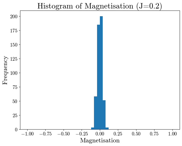
(a) Sub-critical regime

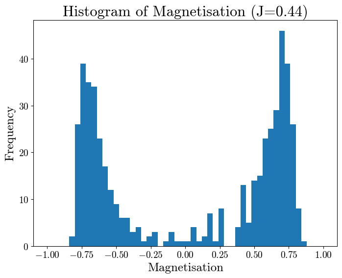
(b) Near-critical regime

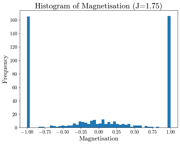
(c) Super-critical regime

Figure 20: Distribution of magnetisation under sub-critical, near-critical and super-critical regimes. 500 simulations run for lattice size $50\times 50$, each simulated for 20 million time steps.

Appendix B Computation of Fisher Information

Let $p(x;\theta)$ denote the probability density of random variable $X$, parameterised by $\theta$. The Fisher information is the variance of the score, and a function of the parameter $\theta$ [61]. The Fisher information can be transformed as follows:

$$\begin{split}\mathbb{I}(\theta)&=\int\left(\frac{\partial\ln p(x;\theta)}{\partial\theta}\right)^{2}p(x;\theta)dx\\ &=\int\left(\frac{\partial p(x;\theta)}{\partial\theta}\right)^{2}\frac{1}{p(x;\theta)}dx\\ &=\int\left(\frac{\partial p(x;\theta)}{\partial\theta}\frac{1}{\sqrt{p(x;\theta)}}\right)^{2}dx\\ &=4\int\left(\frac{\partial\sqrt{p(x;\theta)}}{\partial\theta}\right)^{2}dx\\ \end{split}$$ (46)

In this study, the Fisher information is computed numerically using the discretisation method introduced in [94]:

$$\mathbb{I}(\theta)=4\sum_{x}\left(\frac{\sqrt{p(x;\theta+\Delta\theta)}-\sqrt{p(x;\theta-\Delta\theta)}}{2\Delta\theta}\right)^{2}$$ (47)

References

- Haken [1983] H. Haken, Synergetics: An Introduction, 3rd ed., Springer Series in Synergetics (Springer Berlin, Heidelberg, 1983).
- Haken [2006] H. Haken, Information and Self-Organization: A Macroscopic Approach to Complex Systems, 3rd ed., Springer Series in Synergetics (Springer Berlin, Heidelberg, 2006).
- Camazine et al. [2003] S. Camazine, J.-L. Deneubourg, N. R. Franks, J. Sneyd, G. Theraulaz, and E. Bonabeau, Self-organization in biological systems, Princeton studies in complexity (Princeton University Press, Princeton, NJ, 2003).
- Kauffman [2000] S. A. Kauffman, Investigations (Oxford University Press, New York, 2000).
- Prokopenko et al. [2009] M. Prokopenko, F. Boschetti, and A. J. Ryan, An information-theoretic primer on complexity, self-organization, and emergence, Complexity 15, 11 (2009).
- Beekman et al. [2001] M. Beekman, D. J. T. Sumpter, and F. L. W. Ratnieks, Phase transition between disordered and ordered foraging in Pharaoh’s ants, Proceedings of the National Academy of Sciences 98, 9703 (2001).
- Beggs and Plenz [2003] J. M. Beggs and D. Plenz, Neuronal Avalanches in Neocortical Circuits, The Journal of Neuroscience 23, 11167 (2003).
- Shmulevich et al. [2005] I. Shmulevich, S. A. Kauffman, and M. Aldana, Eukaryotic cells are dynamically ordered or critical but not chaotic, Proceedings of the National Academy of Sciences of the United States of America 102, 13439 (2005).
- Rämö et al. [2006] P. Rämö, J. Kesseli, and O. Yli-Harja, Perturbation avalanches and criticality in gene regulatory networks, Journal of Theoretical Biology 242, 164 (2006).
- Beggs [2008] J. M. Beggs, The criticality hypothesis: How local cortical networks might optimize information processing, Philosophical Transactions of the Royal Society A: Mathematical, Physical and Engineering Sciences 366, 329 (2008).
- Cavagna et al. [2010] A. Cavagna, A. Cimarelli, I. Giardina, G. Parisi, R. Santagati, F. Stefanini, and M. Viale, Scale-free correlations in starling flocks, Proceedings of the National Academy of Sciences 107, 11865 (2010).
- Fessel et al. [2012] A. Fessel, C. Oettmeier, E. Bernitt, N. C. Gauthier, and H.-G. Döbereiner, Physarum polycephalum Percolation as a Paradigm for Topological Phase Transitions in Transportation Networks, Physical Review Letters 109, 078103 (2012).
- Krotov et al. [2014] D. Krotov, J. O. Dubuis, T. Gregora, and W. Bialek, Morphogenesis at criticality, Proceedings of the National Academy of Sciences of the United States of America 111, 3683 (2014).
- Cavagna et al. [2017] A. Cavagna, D. Conti, C. Creato, L. Del Castello, I. Giardina, T. Grigera, S. Melillo, L. Parisi, and M. Viale, Dynamic scaling in natural swarms, Nature Physics 13, 914 (2017).
- Newman [2005] M. Newman, Power laws, Pareto distributions and Zipf’s law, Contemporary Physics 46, 323 (2005).
- Stanley [1971] H. E. Stanley, Introduction to Phase Transitions and Critical Phenomena, 1st ed. (Oxford University Press USA, 1971).
- Halperin and Hohenberg [1969] B. I. Halperin and P. C. Hohenberg, Scaling Laws for Dynamic Critical Phenomena, Physical Review 177, 952 (1969).
- Binney et al. [1992] J. J. Binney, N. J. Dowrick, A. J. Fisher, and M. E. J. Newman, The theory of critical phenomena: an introduction to the renormalization group, Oxford science publications (Clarendon press, Oxford, 1992).
- Bialek et al. [2014] W. Bialek, A. Cavagna, I. Giardina, T. Mora, O. Pohl, E. Silvestri, M. Viale, and A. M. Walczak, Social interactions dominate speed control in poising natural flocks near criticality, Proceedings of the National Academy of Sciences of the United States of America 111, 7212 (2014).
- Stanley et al. [2000] H. E. Stanley, L. A. N. Amaral, P. Gopikrishnan, and V. Plerou, Scale invariance and universality of economic fluctuations, Physica A: Statistical Mechanics and its Applications 283, 31 (2000).
- Bettencourt et al. [2007] L. M. A. Bettencourt, J. Lobo, D. Helbing, C. Kühnert, and G. B. West, Growth, innovation, scaling, and the pace of life in cities, Proceedings of the National Academy of Sciences 104, 7301 (2007).
- Scheffer [2009] M. Scheffer, Critical transitions in nature and society, Princeton studies in complexity (Princeton University Press, Princeton, N.J, 2009).
- Bak et al. [1987] P. Bak, C. Tang, and K. Wiesenfeld, Self-organized criticality: An explanation of the 1/ f noise, Physical Review Letters 59, 381 (1987).
- Drossel and Schwabl [1992] B. Drossel and F. Schwabl, Self-organized critical forest-fire model, Physical Review Letters 69, 1629 (1992).
- Clar et al. [1996] S. Clar, B. Drossel, and F. Schwabl, Forest fires and other examples of self-organized criticality, Journal of Physics Condensed Matter 8, 6803 (1996).
- Malamud et al. [1998] B. D. Malamud, G. Morein, and D. L. Turcotte, Forest fires: An example of self-organized critical behavior, Science 281, 1840 (1998).
- Chen et al. [1991] K. Chen, P. Bak, and S. P. Obukhov, Self-organized criticality in a crack-propagation model of earthquakes, Physical Review A 43, 625 (1991).
- Hesse and Gross [2014] J. Hesse and T. Gross, Self-organized criticality as a fundamental property of neural systems, Frontiers in Systems Neuroscience 8, 10.3389/fnsys.2014.00166 (2014).
- Shew et al. [2015] W. L. Shew, W. P. Clawson, J. Pobst, Y. Karimipanah, N. C. Wright, and R. Wessel, Adaptation to sensory input tunes visual cortex to criticality, Nature Physics 11, 659 (2015).
- Schmidhuber [2010] J. Schmidhuber, Formal Theory of Creativity, Fun, and Intrinsic Motivation (1990–2010), IEEE Transactions on Autonomous Mental Development 2, 230 (2010).
- Oudeyer and Kaplan [2007] P. Y. Oudeyer and F. Kaplan, What is intrinsic motivation? A typology of computational approaches, Frontiers in Neurorobotics 1, 10.3389/neuro.12.006.2007 (2007).
- Ay et al. [2008] N. Ay, N. Bertschinger, R. Der, F. Güttler, and E. Olbrich, Predictive information and explorative behavior of autonomous robots, The European Physical Journal B 63, 329 (2008).
- Der et al. [2008] R. Der, F. Güttler, and N. Ay, Predictive information and emergent cooperativity in a chain of mobile robots, in Proc. Artificial Life XI, edited by S. Bullock, J. Noble, R. Watson, and M. Bedau (MIT Press, Cambridge, MA, 2008) pp. 166–172.
- Zahedi et al. [2010] K. Zahedi, N. Ay, and R. Der, Higher Coordination With Less Control–A Result of Information Maximization in the Sensorimotor Loop, Adaptive Behavior 18, 338 (2010).
- Ay et al. [2012] N. Ay, H. Bernigau, R. Der, and M. Prokopenko, Information-driven self-organization: The dynamical system approach to autonomous robot behavior, Theory in Biosciences 131, 161 (2012).
- Martius et al. [2013] G. Martius, R. Der, and N. Ay, Information Driven Self-Organization of Complex Robotic Behaviors, PLoS ONE 8, 10.1371/journal.pone.0063400 (2013).
- Der and Martius [2013] R. Der and G. Martius, Behavior as broken symmetry in embodied self-organizing robots, in ECAL 2013: The Twelfth European Conference on Artificial Life (MIT Press, Sicily, Italy, 2013) pp. 601–608.
- Der [2014] R. Der, On the Role of Embodiment for Self-Organizing Robots: Behavior As Broken Symmetry, in Guided self-organization: Inception, Emergence, Complexity and Computation, Vol. 9, edited by M. Prokopenko (Springer, Berlin, Heidelberg, 2014) pp. 193–221.
- Klyubin et al. [2005] A. Klyubin, D. Polani, and C. Nehaniv, Empowerment: A Universal Agent-Centric Measure of Control, in 2005 IEEE Congress on Evolutionary Computation, Vol. 1 (IEEE, Edinburgh, Scotland, UK, 2005) pp. 128–135.
- Capdepuy et al. [2007] P. Capdepuy, D. Polani, and C. L. Nehaniv, Maximization of Potential Information Flow as a Universal Utility for Collective Behaviour, in 2007 IEEE Symposium on Artificial Life (IEEE, Honolulu, HI, USA, 2007) pp. 207–213.
- Klyubin et al. [2008] A. S. Klyubin, D. Polani, and C. L. Nehaniv, Keep Your Options Open: An Information-Based Driving Principle for Sensorimotor Systems, PLoS ONE 3, e4018 (2008).
- Capdepuy et al. [2012] P. Capdepuy, D. Polani, and C. L. Nehaniv, Perception-action loops of multiple agents: Informational aspects and the impact of coordination, Theory in Biosciences 131, 149 (2012).
- Salge et al. [2014] C. Salge, C. Glackin, and D. Polani, Empowerment–An Introduction (Springer Berlin Heidelberg, Berlin, Heidelberg, 2014) pp. 67–114, series Title: Emergence, Complexity and Computation.
- Tiomkin et al. [2024] S. Tiomkin, I. Nemenman, D. Polani, and N. Tishby, Intrinsic Motivation in Dynamical Control Systems, PRX Life 2, 033009 (2024).
- Friston et al. [2006] K. Friston, J. Kilner, and L. Harrison, A free energy principle for the brain, Journal of Physiology-Paris 100, 70 (2006).
- Friston [2010] K. Friston, The free-energy principle: A unified brain theory?, Nature Reviews Neuroscience 11, 127 (2010).
- Friston et al. [2015] K. Friston, F. Rigoli, D. Ognibene, C. Mathys, T. Fitzgerald, and G. Pezzulo, Active inference and epistemic value, Cognitive Neuroscience 6, 187 (2015).
- Friston et al. [2017] K. J. Friston, M. Lin, C. D. Frith, G. Pezzulo, J. A. Hobson, and S. Ondobaka, Active Inference, Curiosity and Insight, Neural Computation 29, 2633 (2017).
- Friston et al. [2023] K. Friston, L. Da Costa, N. Sajid, C. Heins, K. Ueltzhöffer, G. A. Pavliotis, and T. Parr, The free energy principle made simpler but not too simple, Physics Reports 1024, 1 (2023).
- Heins et al. [2024] C. Heins, B. Millidge, L. Da Costa, R. Mann, K. Friston, and I. Couzin, Collective behavior from surprise minimization, 121, e2320239121 (2024).
- Crosato et al. [2018a] E. Crosato, R. Nigmatullin, and M. Prokopenko, On critical dynamics and thermodynamic efficiency of urban transformations, Royal Society Open Science 5, 10.1098/rsos.180863 (2018a).
- Crosato et al. [2018b] E. Crosato, R. E. Spinney, R. Nigmatullin, J. T. Lizier, and M. Prokopenko, Thermodynamics and computation during collective motion near criticality, Physical Review E 97, 1 (2018b).
- Harding et al. [2018] N. Harding, R. Nigmatullin, and M. Prokopenko, Thermodynamic efficiency of contagions: A statistical mechanical analysis of the SIS epidemic model, Interface Focus 8, 20180036 (2018).
- Nigmatullin and Prokopenko [2021] R. Nigmatullin and M. Prokopenko, Thermodynamic efficiency of interactions in self-organizing systems, Entropy 23, 757 (2021).
- Stauffer [1992] D. Stauffer, Introduction to Percolation Theory Revised Second Edition, 2nd ed. (Taylor and Francis, London, 1992).
- Stauffer [1979] D. Stauffer, Scaling theory of percolation clusters, Physics Reports 54, 1 (1979).
- Deckmyn et al. [1995] P. Deckmyn, G. Davies, and D. Bell, Properties of percolating clusters on finite lattices applied to model filtration processes, Applied Mathematical Modelling 19, 258 (1995).
- Chen [2024] Q. Chen, qianyangchen/isingmodelpaloop: v1.0.1 (2024).
- Grassberger [2002] P. Grassberger, Critical behaviour of the Drossel-Schwabl forest fire model, New Journal of Physics 4, 17 (2002).
- Palmieri and Jensen [2018] L. Palmieri and H. J. Jensen, The emergence of weak criticality in SOC systems, Europhysics Letters 123, 20002 (2018).
- Cover and Thomas [2005] T. M. Cover and J. A. Thomas, Elements of information theory, 2nd ed. (John Wiley & Sons, Inc., Hoboken, New Jersey, 2005).
- Ay and Zahedi [2013] N. Ay and K. Zahedi, Causal Effects for Prediction and Deliberative Decision Making of Embodied Systems, in Advances in Cognitive Neurodynamics (III), edited by Y. Yamaguchi (Springer, Dordrecht, 2013).
- Ay and Zahedi [2014] N. Ay and K. Zahedi, On the Causal Structure of the Sensorimotor Loop, in Guided Self-Organization: Inception. Emergence, Complexity and Computation, Emergence, Complexity and Computation, Vol. 9, edited by M. Prokopenko (Springer, Berlin, Heidelberg, 2014) pp. 261–294.
- Schmidhuber [1991] J. Schmidhuber, Curious model-building control systems, in 1991 IEEE International Joint Conference on Neural Networks (IEEE, Singapore, 1991) pp. 1458–1463 vol.2.
- Bialek et al. [2001] W. Bialek, I. Nemenman, and N. Tishby, Predictability, complexity, and learning, Neural Computation 13, 2409 (2001).
- Grassberger [1986] P. Grassberger, Toward a quantitative theory of self-generated complexity, International Journal of Theoretical Physics 25, 907 (1986).
- Crutchfield and Young [1989] J. P. Crutchfield and K. Young, Inferring statistical complexity, Physical Review Letters 63, 105 (1989).
- Prokopenko et al. [2006] M. Prokopenko, V. Gerasimov, and I. Tanev, Evolving Spatiotemporal Coordination in a Modular Robotic System, in From Animals to Animats 9, Vol. 4095, edited by S. Nolfi (Springer, Berlin, Heidelberg., Rome, Italy, 2006) pp. 558–569.
- Salge and Polani [2017] C. Salge and D. Polani, Empowerment As Replacement for the Three Laws of Robotics, Frontiers in Robotics and AI 4, 25 (2017).
- Clements and Polani [2017] M. Clements and D. Polani, Empowerment as a Generic Utility Function for Agents in a Simple Team Sport Simulation, in Interactive Collaborative Robotics, Vol. 10459, edited by A. Ronzhin, G. Rigoll, and R. Meshcheryakov (Springer International Publishing, Cham, 2017) pp. 37–49, series Title: Lecture Notes in Computer Science.
- Grasso and Bongard [2022] C. Grasso and J. Bongard, Empowered neural cellular automata, in Proceedings of the Genetic and Evolutionary Computation Conference Companion (ACM, Boston Massachusetts, 2022) pp. 108–111.
- Proietti et al. [2023] R. Proietti, G. Pezzulo, and A. Tessari, An active inference model of hierarchical action understanding, learning and imitation, Physics of Life Reviews 46, 92 (2023).
- Ramstead et al. [2018] M. J. D. Ramstead, P. B. Badcock, and K. Friston, Answering Schrödinger’s question: A free-energy formulation, Physics of Life Reviews 24, 1 (2018).
- Veissière et al. [2020] S. P. L. Veissière, A. Constant, M. J. D. Ramstead, K. J. Friston, and L. J. Kirmayer, Thinking through other minds: A variational approach to cognition and culture, Behavioral and Brain Sciences 43, e90 (2020), publisher: Cambridge University Press.
- Kaufmann et al. [2021] R. Kaufmann, P. Gupta, and J. Taylor, An active inference model of collective intelligence, Entropy 23, 830 (2021).
- Gottwald and Braun [2020] S. Gottwald and D. A. Braun, The two kinds of free energy and the Bayesian revolution, PLOS Computational Biology 16, e1008420 (2020).
- Friston [2009] K. Friston, The free-energy principle: a rough guide to the brain?, Trends in Cognitive Sciences 13, 293 (2009).
- Landauer [1961] R. Landauer, Irreversibility and Heat Generation in the Computing Process, IBM Journal of Research and Development 5, 183 (1961).
- [79] Wikipedia contributors, Thermal Efficiency, accessed: 2024-08-22. Available online: https://en.wikipedia.org/wiki/Thermal_efficiency.
- Brody and Rivier [1995] D. Brody and N. Rivier, Geometrical aspects of statistical mechanics, Physical Review E 51, 1006 (1995).
- Prokopenko et al. [2011] M. Prokopenko, J. T. Lizier, O. Obst, and X. R. Wang, Relating Fisher information to order parameters, Physical Review E - Statistical, Nonlinear, and Soft Matter Physics 84, 041116 (2011).
- Jaynes [1957] E. T. Jaynes, Information Theory and Statistical Mechanics, Physical Review 106, 620 (1957).
- Brody and Ritz [2003] D. C. Brody and A. Ritz, Information geometry of finite Ising models, Journal of Geometry and Physics 47, 207 (2003).
- Janke et al. [2004] W. Janke, D. Johnston, and R. Kenna, Information geometry and phase transitions, Physica A: Statistical Mechanics and its Applications 336, 181 (2004).
- Crooks [2007] G. E. Crooks, Measuring Thermodynamic Length, Physical Review Letters 99, 100602 (2007).
- Bhanot [1988] G. Bhanot, The Metropolis algorithm, Reports on Progress in Physics 51, 429 (1988).
- Janke et al. [2019] W. Janke, H. Christiansen, and S. Majumder, Coarsening in the long-range Ising model: Metropolis versus Glauber criterion, in Journal of Physics: Conference Series, Vol. 1163 (Moscow, Russian Federation, 2019) p. 012002.
- Biehl et al. [2018] M. Biehl, C. Guckelsberger, C. Salge, S. C. Smith, and D. Polani, Expanding the active inference landscape: More intrinsic motivations in the perception-action loop, Frontiers in Neurorobotics 12, 1 (2018).
- Kikuchi [1951] R. Kikuchi, A Theory of Cooperative Phenomena, Physical Review 81, 988 (1951).
- Brandani et al. [2013] G. B. Brandani, M. Schor, C. E. MacPhee, H. Grubmüller, U. Zachariae, and D. Marenduzzo, Quantifying Disorder through Conditional Entropy: An Application to Fluid Mixing, PLoS ONE 8, e65617 (2013).
- Ramaswamy [2010] S. Ramaswamy, The mechanics and statistics of active matter, Annual Review of Condensed Matter Physics 1, 323 (2010).
- Crosato et al. [2019] E. Crosato, M. Prokopenko, and R. E. Spinney, Irreversibility and emergent structure in active matter, Physical Review E 100, 042613 (2019).
- Bialek et al. [2012] W. Bialek, A. Cavagna, I. Giardina, T. Mora, E. Silvestri, M. Viale, and A. M. Walczak, Statistical mechanics for natural flocks of birds, Proceedings of the National Academy of Sciences 109, 4786 (2012).
- Sánchez-Moreno et al. [2009] P. Sánchez-Moreno, R. J. Yanez, and J. S. Dehesa, Discrete Densities and Fisher Information, in Proceedings of the 14th International Conference on Difference Equations and Applications (Bahçesehir University Press, Istanbul, Turkey, 2009) pp. 291–298.