Normal Modes of the Small-Amplitude Oscillon
Jarah Evslin1,2 ***jarah@impcas.ac.cn, Tomasz Romańczukiewicz3 †††tomasz.romanczukiewicz@uj.edu.pl, Katarzyna Sławińska3 ‡‡‡katarzyna.slawinska@uj.edu.pl, and Andrzej Wereszczyński3,4,5 §§§andrzej.wereszczynski@uj.edu.pl
1) Institute of Modern Physics, NanChangLu 509, Lanzhou 730000, China
2) University of the Chinese Academy of Sciences, YuQuanLu 19A, Beijing 100049, China
3) Institute of Theoretical Physics, Jagiellonian University, Lojasiewicza 11, Kraków, Poland
4) Departamento de Matematica Aplicada, Universidad de Salamanca, Spain
5) International Institute for Sustainability with Knotted Chiral Meta Matter (WPI-SKCM2), Hiroshima University, Higashi-Hiroshima, Hiroshima 739-8526, Japan
Abstract
Consider a classical (1+1)-dimensional oscillon of small amplitude . To all orders in , the oscillon solution is exactly periodic. We study small perturbations of such periodic configurations. These perturbations are themselves periodic up to a monodromy matrix. We explicitly find the eigenvectors of the monodromy matrix, which are the analogues of normal modes for oscillons. Dashen, Hasslacher and Neveu used such eigenvectors to quantize the sine-Gordon breather, and we suspect that they will be necessary to quantize the oscillon. Our results, regardless of the chosen model, suggest that low amplitude oscillons do not reflect small amplitude radiation.
1 Introduction
Oscillons [1, 2, 3, 4] are long-lived, quasi-periodic, soliton-like excitations in non-linear field theories. While genuine (large amplitude) oscillons are rather very complicated objects with characteristic double frequency bahaviour and related amplitude modulations, oscillons with a small amplitude seem to be much simpler. Indeed, they are, to all orders in , periodic [5, 6]. This implies [7] that small perturbations about oscillons are also periodic, up to the action of a monodromy matrix.
In Ref. [8] the periodic Sine-Gordon soliton was quantized, using the properties of the monodromy matrix and its eigenvectors. The eigenvectors played the role that was played by normal modes in their earlier quantization of the kink [9]. In the case of quantum kinks, the solutions of these normal modes reproduce the reflection and transmission coefficients for kink-radiation scattering at low amplitudes in classical field theory. Our goal is to do the same for the oscillon, we are interested in both oscillon-radiation scattering and also in the oscillon’s quantization. Thus in the present paper we study the oscillon’s monodromy matrix and its eigenvectors.
Perturbations of oscillons have been studied in the past. Recently, Ref. [10] found a rich structure of perturbations in 2+1 dimensions, as has [11] in 3+1 dimensions. However, with an eye towards quantization, we will restrict our attention to the simplest case of (1+1)-dimensional oscillons. Here, an oscillon whose physical size is enjoys perturbations at several distinct scales. At short wavelengths, of order where is the meson mass, the perturbations are essentially plane waves that scatter with the oscillon. These were studied in Ref. [12] in a rough approximation where the spatial derivatives of the oscillon, and the resonances that they may lead to, were ignored. The stability of wavelength oscillons, whose length scale is similar to the oscillon itself, were investigated in Ref. [13].
Perturbations of large amplitude oscillons are a far more complicated issue. However, it has been recently proposed that such perturbed oscillons, which generically exhibit modulations of amplitude, are in fact bound states of unmodulated oscillons [14]. From this perspective, the perturbed oscillon is a nonlinear superposition of several unperturbed (non-modulated) fundamental oscillons just as the modulated two-breather solution of the sine-Gordon theory is a bound state of two single breathers.
In the present paper, we consider small amplitude oscillons and impose the classical equations of motion up to order , where resonances may first appear and their cancellation places meaningful restrictions on the leading order solutions [6]. We study oscillon perturbations in three regimes. First we study perturbations of wavenumber of order or greater. These we find are essentially plane waves in a potential of Pöschl-Teller form, created by the oscillon. When , if and only if the potential at the vacuum has a cubic term, at leading order there will be relativistic corrections which imply that the Pöschl-Teller potential depends explicitly on . In all cases, we explicitly solve for the leading order perturbations in terms of hypergeometric functions. We find that the symmetric and antisymmetric solutions are out of phase, and so following standard arguments [19], we conclude that in this regime oscillon-radiation scattering is reflectionless for small amplitude radiation.
We also consider a long wavelength regime, where the perturbation has a length scale of order or more. Recall that at leading order the oscillon itself has a behavior. This implies that there is a positive frequency component and a negative frequency component. We find that the perturbations also have two components, one with positive and one with negative frequency. These are described by two Pöschl-Teller equations which are coupled inside of the support of the oscillon. We do not have explicit solutions for these in general. However, for each positive energy we numerically find an even and an odd unbound state. These are asymptotically plane-waves, and by numerically calculating their relative phases we find again that the scattering is reflectionless.
In this long-wavelength regime there are also two zero-modes, which satisfy our coupled equations. One corresponds to the freedom to translate the oscillon, while another corresponds to the phase . On all of the modes mentioned so far, the monodromy matrix can be diagonalized and its eigenvalues are phases, or unity for the zero-modes. However there is also a perturbation corresponding to a moving oscillon. Of course, evolving by one period, the kink motion shifts the kink position zero-mode. Thus the monodromy matrix is not diagonalizable, it is upper triangular.
We also consider intermediate wavenumber perturbations, of order . For these, the positive and negative frequency perturbations decouple at leading order. The relativistic corrections also vanish, and so the leading order perturbations are all hypergeometric functions arising from the same Pöschl-Teller potential. These are just the nonrelativistic limit of those found for the wavenumber perturbations, and so again they result in reflectionless scattering.
An important consequence of our analysis is the fact that small amplitude oscillon do not have discrete massive normal modes.
We begin in Sec. 2 by reviewing the -expansion for the oscillon solution [6]. Next in Sec. 3 we consider relativistic perturbations, with wave number of order or greater. In Sec. 4 we consider intermediate scale perturbations and in Sec. 5 we turn to perturbations of the same length scale as the oscillon itself. Finally in Sec. 6 we describe the perturbation corresponding to a moving oscillon and the monodromy matrix.
2 A Low-Amplitude Oscillon
2.1 The Theory
Let us consider the classical field theory described by a Hamiltonian
| (2.1) |
with the zero of and fixed so that
| (2.2) |
and define
| (2.3) |
Hamilton’s equations are
| (2.4) |
so that
| (2.5) |
We remark that a non-zero mass threshold is not a necessary condition for the existence of oscillons, (it is rather inflection point in the potential or better said an effective potential, see [15],[16] and [17]). However, oscillons in massless models need to have a large amplitude and therefore go beyond the scope of the present work, see [18] for details.
2.2 The Oscillon Solution
Consider the Ansatz
| (2.6) |
where each is of order . If there is such a solution, this Ansatz contains a broad oscillon . The equation of motion can be rewritten as
| (2.7) |
This slight rewriting has an important consequence. The only spatial derivative terms are suppressed by order . This means, that in an expansion, one can solve for each using an ordinary differential equation in time at , as its spatial derivative only appears at . Even at no partial differential equations appear, merely an ordinary differential equation in time for . Now we insert the expansion (2.6) into the equation of motion (2.7).
1 Order
The leading contribution to (2.5) is at
| (2.8) |
which, for real , is solved by
| (2.9) |
for some function of order .
The expansion here is a bit subtle, as in principle can take any value, and may be of order for any , as can the time derivatives. In particular, if is of order then corrections to are of order unity and cannot be relegated to a higher order in the expansion. As a result, our prescription will be as follows. The time-dependence will be exact, in the sense that the frequency of is exactly with no corrections. However, itself will be determined one order at a time. This approach ensures that solutions to the -truncated equations of motion apply at all times .
The in Eq. (2.8) was restricted to . From the solution (2.9) one finds that indeed there are subleading corrections
| (2.10) |
which will appear in the equations at higher orders.
In particular, at order in (2.7), would lead to a resonance. As this is already well known [6], we will simply set . Thus
| (2.11) |
So far, the parameter has been arbitrary. On the other hand, is a physical parameter, corresponding to an observable property of our solution. , on the other hand, is a function of of given by solving Eq. (2.11). Therefore, we are free to transform and drop the prime, so long as is negative. We will make this transformation, restricting our attention to solutions with frequencies below . Whatever dimensions one assigned to before the transformation, had dimensions of , and so after the transformation will have dimensions of mass.
After the transformation, keeping the physical quantity fixed, we find
| (2.12) |
corresponding to .
2 Order
At the next order, Eq. (2.5) becomes
The homogeneous solution for can be absorbed into an contribution to , whereas the particular solution is
| (2.14) |
3 Order
At this order, there is a contribution from
| (2.15) |
Including the term in Eq. (2.15) on the left hand side, one obtains, at the next order
| (2.16) | |||||
In particular, the term proportional to is
| (2.17) |
where the symbol indicates that we restrict to the -dependent piece and we have defined
| (2.18) |
The condition that the resonance vanishes
| (2.19) |
is just the master equation [6], which is solved by
| (2.20) |
where and are constants of integration. The here is equal to in the notation of Ref. [6], as .
The term proportional to is
| (2.21) |
leading to
| (2.22) |
where we have included the identical term with a positive frequency
3 High Energy Perturbations
3.1 The Ansatz
We will first consider perturbations with wave number of order
| (3.1) |
Note that their wavelengths are much shorter than the oscillon wavelength , and so one may expect them to be amenable to a WKB expansion.
We will be interested in the limit
| (3.2) |
for some positive integer . Since we are interested in the linearized solution for , terms of order will be identified with zero.
Note that, up to order , we can ignore terms and so we can trust the expansion above. On the other hand, at order , the equation of motion (2.5) is
| (3.3) |
Inserting
our master formula for perturbations becomes
3.2 Order
The leading order equation for the perturbations is at order
| (3.6) |
A basis of positive frequency solutions is given by
| (3.7) |
Note that is positive as . For now are essentially arbitrary, but their spatial derivatives are suppressed by at least one power of .
| (3.8) |
Later we will need the expansion of out to order
3.3 Order
At the next order, one finds
| (3.10) | |||||
Again the homogeneous solutions for can be rescaled into the coefficients of the functions , leaving the particular solution. The term potentially leads to a resonance. It is a first order, homogeneous ordinary differential equation whose solution contains one constant of integration, that can be interpreted as . We will consider the following solution, which is equivalent to any other choice for some ,
| (3.11) |
3.4 Order
The next order equation is
| (3.16) | |||||
where
| (3.17) | |||||
and
Again, at this order the dependence of is that of the right hand side of (3.16). The derivatives in , at this order, only act on the and so the left hand side is . This means that terms on the right hand side with frequency lead to a resonance. These terms are
| (3.19) |
The resonance is removed by setting the term in the square bracket to zero
| (3.20) | |||||
This fixes to be the solution of this nonrelativistic Schrodinger equation, albeit with a -dependent potential, and leading to the usual small wave number and amplitude shift found for a high frequency wave in a wide, shallow potential . As the potential depends on , or more precisely , one expects that the solutions will not be orthogonal when the perturbation is relativistic, corresponding to of order or greater.
Now one can easily solve for
| (3.21) | |||||
In the nonrelativistic limit, , we find . In particular, the -dependence of the potential disappears, as is expected for a nonrelativistic particle.
3.5 Solving the No-Resonance Condition
The second spatial derivative yields terms at two different orders
| (3.22) |
where the first equality is the definition of the differential operator . One recognizes the last two terms from (3.19)
| (3.23) |
Substituting Eq. (3.23) into the no-resonance condition Eq. (3.20) one finds
This is of the Pöschl-Teller form, although we remind the reader that for each wave number one must choose the potential .
This equation is of the general Pöschl-Teller form
| (3.25) |
Define
| (3.26) |
Then
| (3.27) |
and so
| (3.28) | |||||
To obtain the hypergeometric equation, we need to multiply by for some -dependent
| (3.29) |
Using
| (3.30) |
one finds
where the last equality used the Pöschl-Teller equation Eq. (3.25). Fixing
| (3.32) |
so that
| (3.33) |
the terms cancel in the last equality. This leaves the hypergeometric equation
| (3.34) |
which has coefficients
| (3.35) |
One finds
| (3.36) |
The independent solutions are then
where the sign in the argument of is independent of the sign in the exponent. The sign in the argument, on the other hand, is related to the direction of propagation of the wave.
We remind the reader that
| (3.38) |
Here is a relativistic correction. For long wavelength perturbations it equals , but as the wave number approaches the meson mass, it becomes dependent on the individual couplings and it decreases.
The solutions in this regime have a continuous spectrum, and so any of order corresponds to two solutions. We will fix a unique pair of solutions at each by setting . Then, the term is equal to
| (3.39) |
One may simply replace each with and then check that the asymptotic wavenumber is indeed . Recall that only the asymptotic wavenumber solution, where agrees with the coefficient of , solves the no resonance condition. With this substitution, the solutions are
Using the plus sign, these are the even and odd normal modes of the kink when and the Sine-Gordon soliton when . Note that if an oscillon exists and also . Therefore
| (3.41) |
implies that is monotonically decreasing with respect to . In particular it is greatest at , where , and so it is never equal to .
We can read the reflection and transmission coefficients, as well as the phase shift, off of these functions. For example, the norm squared of the reflection coefficient is given by
| (3.42) |
where and are the asymptotic phases of the even and odd solutions. For the Pöschl-Teller problem with
| (3.43) |
According to Eq. (39.21) of Ref. [19], this phase difference is
| (3.44) |
As a result
| (3.45) |
The treatment in this section is only valid when , a condition which is relaxed in Sec. 5. If is, for example, of order , then is of order and so vanishes in the expansion. More generally, we learn that oscillons do not reflect small-amplitude radiation of wavelength much less than the oscillon width .
Theories with , like the Sine-Gordon model, are much simpler. Then for all . In particular, the normal modes with wave number are solutions of the same Pöschl-Teller problem, and so are orthogonal. It would be interesting to understand how this property relates to the stability of the Sine-Gordon breather.
3.6 Longer Wavelength Perturbations
But what about zero modes and other bound modes? These have compact support and so are not, at leading order, approximated by plane waves . Why were they missed in the treatment above? We assumed that perturbations had wave numbers of order in the Ansatz (3.1). As the only mass scales in the problem are the meson mass and the inverse oscillon length , if the wave number is much larger than it is insensitive to the oscillon and to the mass and so is as in the free theory. On the other hand, a smaller wave number invalidates the expansion above.
4 Intermediate Wave Number Perturbations
The derivation above fails already for a perturbation with wave number , as the kinetic energy term enters only at order .
More precisely, consider the Ansatz
| (4.1) |
Then at order instead of (3.6) one finds
| (4.2) |
This is solved by
| (4.3) |
for some function . Here labels the solution. In particular, up to order
| (4.4) |
Next, at order , Eq. (2.5) becomes
| (4.5) | |||||
The terms lead to a naive resonance unless
| (4.6) |
As a result, a basis of solutions is
| (4.7) |
We see that is an ordinary plane wave solution, as in the high energy perturbations. This is to be expected, as the wavelength of the perturbations is still much less than the length of the oscillon. Note that is of order as and are both of order by definition.
Summarizing, we have found
| (4.8) | |||||
where is a homogeneous solution. We will see shortly that the only part of the homogeneous solution needed to remove the leading resonance is
| (4.9) |
One may choose to interpret as the correction to in Eq. (4.7)
| (4.10) |
Let us proceed to order , where we have seen that resonances can appear. Now the equation of motion is
| (4.11) | |||||
Resonances can arise both from terms proportional to and also those proportional to . The terms proportional to are
| (4.12) |
The resonance is therefore canceled if
| (4.13) |
This is easily solved by Fourier transform. The Fourier transform of this equation is
| (4.14) |
This leads to
| (4.15) |
Now recall that is of order . Therefore the in the argument of csch is of order unless . Note that the pole in csch at is canceled by the numerator of the previous term. As the csch term leads to an exponential suppression when is outside of window whose size is of order , the integration is over a domain of size and so leads to a factor of order . As a result, itself is of order . However, by definition is a term in which is of order , and so its order corrections are meaningless. One could define them to be the homogeneous part of , but these will be constrained by the resonance condition at , which we do not consider. Thus, we set .
This is to be expected, as the resonance is caused by
| (4.16) |
but the characteristic length scale of is and that of the phase term is . This means that the phase oscillates of order times over the length of the oscillon, leading to destructive interference which already essentially eliminates this potential resonance. There would not be so much interference if were of order , in which case the perturbation length scale would the same as that of . We next turn to that case in Sec. 5. For now, as the term is exponentially suppressed we will ignore it.
The other resonance corresponds to terms proportional to . These are
| (4.17) | |||||
The vanishing of the square brackets is again a linear ordinary differential equation for which can be solved by Fourier transform. Rewriting this as a homogeneous equation for in the form (4.10), one can identify this as the part of a time-independent, non-relativistic Schrodinger equation for a monochromatic wave in a potential well
| (4.18) | |||||
Note that this agrees with the nonrelativistic limit of Eq. (3.5), with here identified with there. We conclude that intermediate wavelength perturbations are described by the same formulas as the short wavelength perturbations found in the previous section, which is of little surprise as both have wavelengths which are much shorter than the oscillon.
5 Long Wavelength Perturbations
5.1 Zero Modes
To find honest, bound modes one needs a wave number which is still lower. The analysis above fails once the wave number falls to order However, if depends on position via the combination and it has the same frequency as the oscillon , then its dependence matches that of in Eq. (3.1). Therefore, any frequency solution in this regime, can be obtained by setting and absorbing it into In other words, all such perturbations of wavelength are already contained in the analysis of Subsec. 2.2. In particular, any solution plus such periodic perturbations should correspond to a solution of the master equation Eq. (2.19).
The solutions of Eq. (2.19) are
| (5.1) |
These depend on two constants of integration. The first is , the position of the center of the oscillon. The second is the phase . The analogues of zero modes for the oscillon are just the small perturbations in these constants of integration. In other words, up to normalization constants that may be fixed at will, spatial translations and time translations correspond to the zero modes
| (5.2) |
where is the sum of all up to the desired order.
Note that the term zero mode is rather misleading, as these have frequencies of , which is approximately , not zero. Indeed they are a long wavelength limit of the meson in which the meson no longer fits entirely inside of the oscillon. In particular, it may be that there is no gap between these zero modes and the continuum.
At leading order is simply where
| (5.3) |
Therefore the zero modes are
| (5.4) |
5.2 General Long Wavelength Perturbations
We have discovered that there are two perturbation modes, and , which have the same frequency as the oscillon. They have compact support, and frequencies below the threshold , and so presumably they are discrete states. However, our analysis of the continuum modes was only valid for wavenumbers with , and so we have not shown that the frequencies of the continuum modes do not extend down to .
Recall that in the case of modes with wavenumbers of order , the kinetic term, and so the nontrivial constraints, only appear at order . Here, the corrections to the frequency also appear. Thus our above treatment of the expansion at does not apply when the wavenumber is of order .
Such perturbations need to be considered if one wishes to see whether the set of indeed forms a basis of the set of functions, as is needed to decompose the Schrodinger picture fields and . For example, one may search for a completeness relation similar to (2.13) in Ref. [20].
With this motivation, let us consider the expansion of a new Ansatz
| (5.5) |
which is suitable for long wavelength perturbations. We expect and to be solutions. Now the terms are as above, but we will allow for different relativistic corrections to the frequency of the perturbations. Therefore the terms will differ.
At order the equation of motion is just Eq. (4.2). However, we now write a solution, indexed by , as
| (5.6) |
for some which is equal to
| (5.7) |
The solutions and would arise at The term here plays the same role as in the homogeneous solution in in the case of intermediate scale perturbations. Here it is one order lower in , appearing in instead of , because two derivatives now lead to an additional power of .
Using
| (5.8) |
one finds
At order we arrive at
Every term in the second line has a frequency of or and so does not lead to a resonance. On the other hand, the terms in the first line have frequency and so do lead to a resonance unless . Therefore we fix .
Again the homogeneous solution for may be absorbed into corrections to and . The particular solution is
As in the usual expansion, the most interesting order has three powers of , as that is the first place where spatial derivatives appear and so constraints may be placed on the spatial functions. At one finds
where the denotes that we dropped the terms, as they do not contribute to any resonance.
The terms proportional to are
| (5.13) |
while those proportional to are
| (5.14) |
We learn that the resonances vanish when two coupled, linear ordinary differential equations are satisfied
| (5.15) | |||||
Choosing or , which is just an arbitrary choice of initial time , this is
| (5.16) | |||||
5.3 Solutions of Eq. (5.15)
Eq. (5.15) simplifies to a very elegant form if we define
| (5.17) |
Indeed, using
| (5.18) |
one finds that the second equation plus (minus) times the first gives
| (5.19) | |||||
These are two coupled equations of the Pöschl-Teller form, where the coupling is given by simply, constant coefficient terms.
These functions may be decomposed in a basis of eigenfunctions of the corresponding ordinary Pöschl-Teller problems
| (5.20) |
where here represents a sum over all continuum and bound modes, including zero modes, of the corresponding problem. More precisely, where the index may be a continuum mode or while may be a continuum mode, or .
The modes satisfy the Sturm-Liouville problems
| (5.21) |
where for concreteness we have set .
Inserting this basis into the equations of motion Eq. (5.19) one finds
| (5.22) | |||||
where we have defined
| (5.23) |
Note that is not the frequency of any particle, as is not a mass, rather it is a kind of effective energy for a long wavelength perturbation of the oscillon. The sums on the left hand side contain all bound modes. However if then the left hand side vanishes and so and , the coefficients of and , do not appear in the equations. As a result, and are zero-mode solutions.
1 Zero Modes
Consider the special case . In this case, these coupled equations are easily solved. Indeed, the equations decouple
| (5.24) |
| (5.25) |
These are the and Pöschl-Teller equations with energy . This energy corresponds to the highest bound state in each case.
In other words, if then is the higher of the two bound states, and, using the known solution, one finds that is the temporal zero mode. On the other hand, if then is the only bound state, and it yields the spatial zero mode .
5.4 Near Threshold Continuum Modes
1 Continuum Modes
Consider , so that the terms in Eq. (5.15) vanish
| (5.26) |
We expect, based on intuition with time-independent backgrounds, that only negative frequency modes will be interesting. Therefore we restrict our attention to . Then we see that always falls off exponentially far from the oscillon, however becomes a plane wave for , corresponding to and so the frequency of beyond the mass threshold. It remains to check that these lead to consistent solutions to (5.15).
When , is continuous and is bound, so in principle for a given there may be several solutions corresponding to different numbers of nodes of . We have numerically obtained a branch of solutions for all frequencies in this regime, some of which are plotted in Figs. 1 and 2 at .
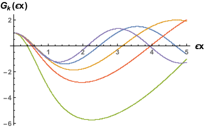
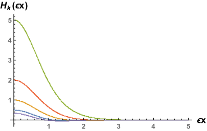
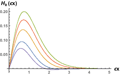
At higher frequencies, becomes smaller. This is consistent with the fact that at very lower frequencies, in Sec. 4, we saw in Eq. (4.15) that it is suppressed. Note that in the case of the even perturbations the -intercepts of are, within numerical errors, equal to
| (5.27) |
Indeed, close to the threshold at , we find that tends to . Similarly, in the case of the odd functions, the slopes at the origin are related by
| (5.28) |
This gives hope that analytic solutions may be found. We also note that the even and odd solutions appear to be 90 degrees out of phase far from the oscillon, and so may be assembled into or , suggesting that reflectionless oscillon-radiation scattering persists even at these long wavelengths.
6 Nonperiodic Solutions
6.1 A Moving Oscillon
We have not yet found all solutions of Eq. (3.3), as we have assumed that equals up to a phase. Another solution is provided by a moving oscillon. In the defining frame, this can be constructed by simply boosting the oscillon solution
| (6.1) |
In the comoving frame this is
| (6.2) |
Recalling that and are solutions of (3.3), we can check that is a solution
Note that this solution corresponds to the initial conditions
| (6.4) |
In the case of the moving kink, and so only the term in appears. Returning to the general oscillon case, instead of periodicity, satisfies the condition
6.2 The Monodromy Matrix
Following the general treatment of perturbations of stable orbits in Ref. [7], we may define a monodromy matrix such that
| (6.6) |
The vectors are eigenvectors, as are
| (6.7) |
where the second equation is the complex conjugate of the first, using the fact that is real. Similarly the zero-modes are preserved by
| (6.8) |
Finally Eq. (6.1) implies
| (6.9) |
Note that is not diagonalizable, in fact on the basis it is upper-triangular. Nonetheless, the monodromy matrix acts on all perturbations and so vectors span the space of pairs of functions, corresponding to arbitrary initial conditions. The pairs corresponding to and are linearly independent and, if they span the space of solutions of (3.3), then these pairs are a basis of the space of pairs of functions. This means that they can be used to decompose Schrodinger picture pairs in quantum field theory and so will allow a quantization of the oscillon following the strategy of Refs. [21, 22].
7 Remarks
In classical field theory, oscillons dominate configurations fairly ubiquitously [2, 23, 24, 25, 26] after violent events have excited all perturbations, and short-lived perturbations have had time to dissipate. As a result, oscillons play a key role in many phenomenological contexts [27, 28, 29, 30]. It is often claimed that this is not the case in the real world, as the quantum oscillons of Refs. [31, 32, 33] emit radiation with such a high luminosity, of order the meson mass squared, that, if they continued to radiate, they would dissipate rather quickly.
The key question becomes, what is the end point of this decay? Is it pure radiation or a more stable quantum oscillon? This motivates us to search for a more stable quantum oscillon than that of Refs. [31, 32], see e.e., [34] and thus our interest in the quantization of oscillon.
We wish not only to find the quantum corrections to the oscillon mass, as in the treatment of breathers in Ref. [8], but we also desire to explicitly find the oscillon state. This will allow us to answer questions such as whether the phase can be fixed for a quantum oscillon, or rather whether it is necessarily described by some continuous wave functions. Or, more likely, whether it smears over a time scale which is suppressed in powers of the coupling . To do this, we will use the approach of Refs. [21, 22, 20]. But this approach, as well as that of Ref. [8], requires the full monodromy matrix. In particular, one needs to find explicit expressions for a set of perturbations which spans the space of initial conditions, consisting of all possible perturbations of the field and its first time derivative. In the case of the quantum kink, the perturbations were described by a Sturm-Liouville equation, whose solutions are known to provide a basis. However in the present case, we have not yet shown completeness for our solutions. Perhaps this needs to be done numerically. Nonetheless, numerically we have searched and we have not found other solutions.
In summary, we have classified the perturbations of the small amplitude oscillon and we have numerical evidence that our classification is complete. We stress that our analysis applies to models with any potential which admits a small amplitude oscillon solution, which in particular requires that the mass threshold be nonzero. If the solutions found here are indeed complete, then we are now ready to quantize the oscillon.
Interestingly, the non-existence of massive bound modes for oscillons provides a further support for the recently proposed explanation of amplitude modulation. A genuine oscillon enjoys two independent degrees of freedom: the fundamental frequency and a frequency of the amplitude modulations. In [14] it has been argued that modulated oscillon can be viewed as a semi-bound state of two (or more) unmodulated, fundamental oscillons. Potentially, one might imagine another explanation where the one parameter expansion [6] gives the fundamental frequency while a linear perturbation leads to an internal vibrational mode which is the second degree of freedom needed for the modulations. Since small amplitude oscillons do not host vibrational modes this possibility is excluded.
Acknowledgements
KS acknowledge financial support from the Polish National Science Centre (Grant NCN 2021/43/D/ST2/01122).
References
- [1] I. L. Bogolyubsky and V. G. Makhankov, “Lifetime of Pulsating Solitons in Some Classical Models,” Pisma Zh. Eksp. Teor. Fiz. 24 (1976), 15-18
- [2] M. Gleiser, “Pseudostable bubbles,” Phys. Rev. D 49 (1994), 2978-2981 doi:10.1103/PhysRevD.49.2978 [arXiv:hep-ph/9308279 [hep-ph]].
- [3] M. Gleiser, Oscillons in scalar field theories: Applications in higher dimensions and inflation, Int. J. Mod. Phys. D 16 (2007) 219.
- [4] M. Gleiser and D. Sicilia, A General Theory of Oscillon Dynamics, Phys. Rev. D 80 (2009) 125037.
- [5] A. M. Kosevich and A. S. Kovalev, “Self-localization of vibrations in a one-dimensional anharmonic chain.” Zh. Eksp. Teor. Fiz. 67 (1974) 1793-1804
- [6] G. Fodor, P. Forgacs, Z. Horvath and A. Lukacs, “Small amplitude quasi-breathers and oscillons,” Phys. Rev. D 78 (2008), 025003 doi:10.1103/PhysRevD.78.025003 [arXiv:0802.3525 [hep-th]].
- [7] L. A. Pars, “A Treatise on Analytical Dynamics,” (Heinemann, London, 1965)
- [8] R. F. Dashen, B. Hasslacher and A. Neveu, “The Particle Spectrum in Model Field Theories from Semiclassical Functional Integral Techniques,” Phys. Rev. D 11 (1975), 3424 doi:10.1103/PhysRevD.11.3424
- [9] R. F. Dashen, B. Hasslacher and A. Neveu, “Nonperturbative Methods and Extended Hadron Models in Field Theory 2. Two-Dimensional Models and Extended Hadrons,” Phys. Rev. D 10 (1974) 4130. doi:10.1103/PhysRevD.10.4130
- [10] Y. J. Wang, Q. X. Xie and S. Y. Zhou, “Excited oscillons: cascading levels and higher multipoles,” Phys. Rev. D 108 (2023) 025006.
- [11] F. van Dissel, O. Pujolas and E. Sfakianakis, “Oscillon spectroscopy,” JHEP 07 (2023) 194.
- [12] M. A. Amin, “Inflaton fragmentation: Emergence of pseudo-stable inflaton lumps (oscillons) after inflation,” [arXiv:1006.3075 [astro-ph.CO]].
- [13] F. Van Dissel, “Multi-Component Oscillons,” Masters Thesis at Leiden University, 2020, https://hdl.handle.net/1887/135806.
- [14] F. Blaschke, T. Romanczukiewicz, K. Slawinska, and A. Wereszczynski, ”Amplitude modulations and resonant decay of excited oscillons”, Phys. Rev. E 110 (2024) 014203 [arXiv:2403.00443 [hep-th]].
- [15] M. Gleiser and D. Sicilia, ”Analytical Characterization of Oscillon Energy and Lifetime” Phys. Rev. Lett. 101, 011602 doi.org/10.1103/PhysRevLett.101.011602 [arXiv:0804.0791 [hep-th]]
- [16] E. J. Copeland, M. Gleiser, and H.-R. Müller ”Oscillons: Resonant configurations during bubble collapse” Phys. Rev. D 52, 1920 doi.org/10.1103/PhysRevD.52.1920 [arXiv:hep-ph/9503217 [ht-ph]]
- [17] G. Fodor, P. Forgacs, Z. Horvath, and Mark Mezei, ”Computation of the radiation amplitude of oscillons”, Phys. Rev. D 79 (2009) 065002.
- [18] P. Dorey, T. Romanczukiewicz, Y. Shnir, A. Wereszczynski, ”Oscillons in gapless theories”, Phys. Rev. D 109 (2024) 085017 [arXiv:2312.05308 [hep-th]].
- [19] S. Flügge, “Practical Quantum Mechanics,” Springer-Verlag Berlin Heidelberg (1999), doi:10.1007/978-3-642-61995-3
- [20] J. Evslin and H. Guo, “Two-Loop Scalar Kinks,” Phys. Rev. D 103 (2021) no.12, 125011 doi:10.1103/PhysRevD.103.125011 [arXiv:2012.04912 [hep-th]].
- [21] K. E. Cahill, A. Comtet and R. J. Glauber, “Mass Formulas for Static Solitons,” Phys. Lett. B 64 (1976), 283-285 doi:10.1016/0370-2693(76)90202-1
- [22] J. Evslin, “Manifestly Finite Derivation of the Quantum Kink Mass,” JHEP 11 (2019), 161 doi:10.1007/JHEP11(2019)161 [arXiv:1908.06710 [hep-th]].
- [23] V. A. Gani, A. M. Marjaneh and K. Javidan, “Exotic final states in the multi-kink collisions,” Eur. Phys. J. C 81 (2021) no.12, 1124 doi:10.1140/epjc/s10052-021-09935-7 [arXiv:2106.06399 [hep-th]].
- [24] X. Li and L. Long, “Radiation-like Shock Waves in Kink Scattering,” [arXiv:2407.14479 [hep-th]].
- [25] S. Navarro-Obregon, L. M. Nieto, and J. M. Queiruga, Inclusion of radiation in the CCM approach of the model, Phys. Rev. E 108 (2023) 044216.
- [26] F. C. Lima, F. C. Simas, K. Z. Nobrega, and A. R. Gomes, Scattering of metastable lumps in a model with a false vacuum, Phys. Lett. B 822 (2021) 136707.
- [27] K. D. Lozanov, M. Sasaki and V. Takhistov, “Universal Gravitational Wave Signatures of Cosmological Solitons,” [arXiv:2304.06709 [astro-ph.CO]].
- [28] J. C. Aurrekoetxea, K. Clough and F. Muia, “Oscillon formation during inflationary preheating with general relativity,” Phys. Rev. D 108 (2023) 023501 .
- [29] D. Pîrvu, M. C. Johnson and S. Sibiryakov, “Bubble velocities and oscillon precursors in first order phase transitions,” [arXiv:2312.13364 [hep-th]].
- [30] D. del-Corral, “Self-resonance after inflation: The case of -attractor models,” [arXiv:2406.04017 [hep-th]].
- [31] M. P. Hertzberg, “Quantum Radiation of Oscillons,” Phys. Rev. D 82 (2010), 045022 doi:10.1103/PhysRevD.82.045022 [arXiv:1003.3459 [hep-th]].
- [32] J. Ollé, O. Pujolas, T. Vachaspati and G. Zahariade, “Quantum Evaporation of Classical Breathers,” Phys. Rev. D 100 (2019) no.4, 045011 doi:10.1103/PhysRevD.100.045011 [arXiv:1904.12962 [hep-th]]
- [33] M. Mukhopadhyay, E. I. Sfakianakis, T. Vachaspati and G. Zahariade, “Kink-antikink scattering in a quantum vacuum,” JHEP 04 (2022), 118 doi:10.1007/JHEP04(2022)118 [arXiv:2110.08277 [hep-th]].
- [34] J. Evslin, T. Romanczukiewicz and A. Wereszczynski, ”Quantum Oscillons May be Long-Lived”, JHEP 08 (2023) 182 [arXiv:2305.18056 [hep-th]].