Revealing the propagation dynamic of Laguerre-Gaussian beam with two Bohm-like theories

Abstract

By employing $x$-Bohm theory and $p$-Bohm theory, we construct the position and momentum trajectories of single-mode and superposed-mode Laguerre-Gaussian (LG) beams. The dependence of divergence velocity and rotation velocity on the initial position and propagation distance is quantified, indicating that LG beams exhibit subluminal effects, even in free space. Additionally, we clarify the formation of the petal-shaped intensity distribution of the superposed-mode LG beam in terms of motion trajectory, where the particle-like trajectory and wave-like interference are “simultaneously" observed. Our work provides an intuitive way to visualize the propagation characteristics of LG beams and deepen the comprehension of Bohm-like theory.

1 Introduction

Laguerre-Gaussian (LG) beams, a typical type of vortex beams carrying orbital angular momentum (OAM), are renowned for the infinite OAM orthogonal modes and spiral phase structure [1]. They have been widely used in optical communication [2, 3, 4], particle manipulation [5, 7, 6], super-resolution imaging [8, 9, 10], quantum information processing [13, 14, 11, 12], and various other domains [17, 16, 15]. These promising applications of LG beams have driven significant advancements in their generation and detection techniques [18, 19, 20, 21, 22]. Moreover, several adaptive optical methods have been devised to recover LG beams distorted by atmospheric or ocean turbulence [23, 24]. Despite all these works, investigations into the mechanisms and physics underlying their propagation remain limited. Most existing studies have approached this subject from a classical wave-optics analysis [25, 26]. Further research is needed from a trajectory viewpoint, considering the wave-particle duality, to gain insight into the propagation characteristics inherent in different LG beams. For instance, it is crucial to investigate why LG beams exhibit slow-light effects, even in free space [27, 28]; determine the quantitative relationship between beam parameters and propagation velocity; and elucidate how the petal-shaped intensity distribution of superposed-mode LG beams forms and evolves.

In standard quantum mechanics, the Heisenberg uncertainty principle suggests that it is impossible to simultaneously determine the position and momentum of a particle [29]. This implies that accurately tracking the trajectory of a quantum particle, as we can with a classical particle, is unattainable. Nevertheless, in 1952, Bohm proposed a nonlocal hidden-variable interpretation of quantum theory, predicting that a particle has a deterministic trajectory guided by the position space wave function [30, 31]. In Bohm’s interpretation, the position variable is regarded as the primary ontological variable. The momentum of a particle is simply derived from its velocity, which is determined by the gradient of the wavefunction at the corresponding position. Considering the equal importance of position and momentum inherent in both classical and quantum mechanics, Epstein later proposed an alternative trajectory theory, where momentum acts as the primary ontological status and a particle’s trajectory is fundamentally characterized by its momentum space wavefunction [32, 33]. For simplicity, we refer to Bohm’s original theory as $x$-Bohm theory and Epstein’s proposal as $p$-Bohm theory. Subsequently, Wiseman demonstrated that velocities of Bohm-like particles can be experimentally extracted by taking conditional averages of weak measurements on an ensemble of post-selected systems [34]. Inspired by his idea, researchers have successfully obtained putative Bohmian trajectories in various two-slit experiments [35, 36, 37, 38, 39]. However, the propagation dynamics of LG beams, particularly that of superposed-mode LG beams, have been rarely analyzed from the perspective of Bohm-like trajectories.

In this work, we explore the propagation trajectories of single-mode and superposed-mode LG beams within the frameworks of both $x$-Bohm theory and $p$-Bohm theory. We investigate the subluminal effect of these beams concerning the initial position and the propagation distance. Additionally, the formation of petal-shaped intensity distributions of superposed-mode LG beams is clarified by the motion trajectory. Notably, we find that both the position trajectory and the momentum trajectory exhibit significantly different dynamics in $x$-Bohm theory and $p$-Bohm theory. Our trajectory-baesd method not only provides an intuitive depiction of the propagation characteristics of LG beams but can also be extended to describe the properties of arbitrarily structured light beams, including propagation behavior, spin-orbit and orbit-orbit interactions, as well as diffraction and interference phenomena. Additionally, by employing the weak measurement techniques mentioned in the references [39, 40], it can also experimentally reconstruct the corresponding trajectories.

2 Theoretical Model

We start by reviewing the $x$-Bohm theory and $p$-Bohm theory, and then derive the trajectories of the primary and non-primary ontological variables of the particles in each theory. This enables us to quantify the difference between the two theories by contrasting their predicted trajectories in the same space.

2.1 the trajectory in $x$-Bohm theory

In $x$-Bohm theory, the primary and non-primary ontological variables are respectively identified as the position and momentum of the particle, with the fundamental dynamics occurring in position space [30, 31]. Assuming the particle’s position wave function is $\psi(\textbf{x},t)=R(\textbf{x},t){\rm exp}(iS(\textbf{x},t)/\hbar)$, its velocity is given by

$$\textbf{v}(\textbf{x},t)=\nabla S(\textbf{x},t)/m,$$ (1)

where $\nabla$ is the gradient operator in position space, $m$ is the mass of the particle, and $R(\textbf{x}(t),t)$ and $S(\textbf{x}(t),t)$ are the amplitude and phase functions, respectively. As the wave function $\psi(\textbf{x},t)$ evolves according to the Schrödinger equation

$$i\hbar\dfrac{\partial}{\partial t}\psi(\textbf{x},t)=\dfrac{\hat{\textbf{p}}^{2}}{2m}\psi(\textbf{x},t)+\hat{V}(\textbf{x})\psi(\textbf{x},t).$$ (2)

Here, $\hat{\textbf{p}}=-i\hbar\nabla$ is the momentum operator. Eq. (3) can be rewritten as

$$\textbf{v}(\textbf{x},t)=\dfrac{\textbf{j}(\textbf{x},t))}{|\psi(\textbf{x},t))|^{2}},$$ (3)

where $\textbf{j}(\textbf{x},t)$ represents the probability current and can be expressed as

$$\begin{split}\textbf{j}(\textbf{x},t)=\dfrac{1}{2m}(\psi^{\ast}(\textbf{x},t)\hat{\textbf{p}}\psi(\textbf{x},t)-\psi(\textbf{x},t)\hat{\textbf{p}}\psi^{\ast}(\textbf{x},t)).\end{split}$$ (4)

In analogy to classical Newtonian mechanics, the position trajectory of a particle in the $x$-Bohm theory is determined by its initial position $\textbf{x}_{0}$ and the integral of its velocity over time. The guidance equation for the position trajectory can be written as

$$\begin{split}\textbf{x}(t)=\textbf{x}_{0}+\int^{t}_{0}\textbf{v}(\textbf{x},t)dt.\end{split}$$ (5)

Clearly, for a particle at position $\textbf{x}(t)$ at time $t$, the momentum of the particle can be obtained by multiplying its velocity by its mass, i.e.,

$$\begin{split}\textbf{p}(\textbf{x}(t),t)=m\textbf{v}(\textbf{x}(t),t).\end{split}$$ (6)

From an experimental perspective, Wiseman et al. have shown that Eq. (6) can be expressed in terms of the weak value as follows:

$$\begin{split}\textbf{p}(\textbf{x}(t),t)={\rm Re}\dfrac{\langle\textbf{x}(t)|\hat{\textbf{p}}|\psi(t)\rangle}{\langle\textbf{x}(t)|\psi(t)\rangle}=\hbar\cdot{\rm Im}\dfrac{\nabla\psi(\textbf{x}(t),t)}{\psi(\textbf{x}(t),t)}.\\ \end{split}$$ (7)

By tracking $\textbf{p}(\textbf{x}(t),t)$ as $t$ evolves, one can assign a momentum trajectory to the particle in the $x$-Bohm theory.

2.2 the trajectory in $p$-Bohm theory

The $p$-Bohm theory offers a different perspective on the dynamic behavior of a particle, wherein the momentum and position of the particle are identified as the primary and non-primary ontological variables, respectively [32, 33]. Clearly, its fundamental dynamics take place in momentum space. The particle’s wave function in the momentum representation can be expressed as $\widetilde{\psi}(\textbf{p},t)=\int^{\infty}_{-\infty}d^{3}x\psi(\textbf{x},t)e^{-i\textbf{p}\cdot\textbf{x}/\hbar}$ and is guided by the Schrödinger equation

$$i\hbar\dfrac{\partial}{\partial t}\widetilde{\psi}(\textbf{p},t)=\dfrac{\hat{\textbf{p}}^{2}}{2m}\widetilde{\psi}(\textbf{p},t)+\hat{V}(i\hbar\nabla_{p}\widetilde{\psi}(\textbf{p},t)),$$ (8)

where $\nabla_{p}$ is the gradient operator in momentum space. Unlike Eq. (2) involves only second derivatives with respect to $x$, Eq. (8) can involve any number of derivatives with respect to $p$, potentially giving rise to distinct trajectories in $p$-Bohm theory.

Similarly, the evolution of the particle’s momentum trajectory is determined by the guidance equation

$$\begin{split}\textbf{p}(t)=\textbf{p}_{0}+\int^{t}_{0}\textbf{v}(\textbf{p},t)dt=\textbf{p}_{0}+\int^{t}_{0}\dfrac{\textbf{j}(\textbf{p},t)}{|\widetilde{\psi}(\textbf{p},t)|^{2}}dt,\end{split}$$ (9)

where $\textbf{p}_{0}$ is the initial momentum, $\textbf{v}(\textbf{p},t)=\textbf{j}(\textbf{p},t)/|\widetilde{\psi}(\textbf{p},t)|^{2}$ is the corresponding velocity, and $\textbf{j}(\textbf{p},t)$ is the probability current, writing

$$\begin{split}\textbf{j}(\textbf{p},t)=\dfrac{2}{\hbar}\int^{p}_{-\infty}{\rm Im}[\widetilde{\psi}(\textbf{p}^{\prime},t)^{\ast}V(i\hbar\nabla_{p^{\prime}})\widetilde{\psi}(\textbf{p}^{\prime},t)]d^{3}p^{\prime}.\end{split}$$ (10)

It satisfies the physically reasonable assumption that $\textbf{j}(\textbf{p},t)\rightarrow 0$ as $|\textbf{p}|\rightarrow\infty$.

Analogous to Eq. (7), for a particle with momentum $\textbf{p}(t)$ at time $t$, the position of the particle can be expressed as

$$\begin{split}\textbf{x}(\textbf{p}(t),t)={\rm Re}\dfrac{\langle\textbf{p}(t)|\hat{\textbf{x}}|\widetilde{\psi}(t)\rangle}{\langle\textbf{p}(t)|\widetilde{\psi}(t)\rangle}=-\hbar\cdot{\rm Im}\dfrac{\nabla_{p}\widetilde{\psi}(\textbf{p}(t),t)}{\widetilde{\psi}(\textbf{p}(t),t)}.\\ \end{split}$$ (11)

By tracking $\textbf{x}(\textbf{p}(t),t)$ as $t$ evolves, one can assign a position trajectory to the particle in the $p$-Bohm theory.

It is noteworthy that the energy flow trajectories [25, 26], employed in previous investigations on the propagation of LG beams, are essentially similar to the position trajectories in position space. By combining $x$-Bohm theory with $p$-Bohm theory, an in-depth exploration of the position trajectory in momentum space, along with the momentum trajectory in both position and momentum spaces, becomes feasible. Subsequently, a comprehensive analysis of LG beam propagation trajectory in three-dimensional space will be conducted to achieve a more thorough understanding of its dynamics.

3 the trajectory of LG Beam

In position space, the time-dependent wave function (or complex amplitude at the propagation distance $z$) of a single-mode LG beam with an angular momentum index $l$ and a radial mode index $p$ can be expressed as [1]

$$\begin{split}LG^{l}_{p}(r,{\theta},z)&=\sqrt{\dfrac{2p!}{\pi(p+|l|)!}}\frac{1}{\omega_{z}}(\dfrac{\sqrt{2}r}{\omega_{z}})^{|l|}{\rm exp}(\dfrac{-r^{2}}{\omega_{z}^{2}})\times\\ &L^{|l|}_{p}(\dfrac{2r^{2}}{\omega_{z}^{2}}){\rm exp}(-\dfrac{ikr^{2}z}{2(z^{2}+z^{2}_{R})}-il{\theta}+i\xi_{g}+ikz),\end{split}$$ (12)

where $(r,\theta)$ are the polar coordinates, $k=2\pi/\lambda$ is the wave number, $\lambda$ is the wavelength, $z_{R}=\pi\omega_{0}^{2}/\lambda$ is the Rayleigh length, $\omega_{z}=\omega_{0}\sqrt{1+(z/z_{R})^{2}}$ is the beam waist radius at the propagation distance $z$, $L^{|l|}_{p}(\cdot)$ the associated Laguerre polynomial, $\xi_{g}=(2p+|l|+1){\rm arctan}({z}/z_{R})$ is the Gouy phase, and ${\rm exp}(il\theta)$ is the spiral phase term. For simplicity, we consider an LG beam with a radial mode index $p=0$. The wave function of the LG beam in momentum space is obtained by applying the Fourier transform to its position space wave function, which can be expressed as

$$\begin{split}\widetilde{LG}^{l}_{0}(\rho,\varphi,z)&=\sqrt{\dfrac{2\pi}{|l|!}}\omega_{0}(-i)^{|l|}(\sqrt{2}\pi\omega_{0}\rho)^{|l|}\times\\ &{\rm exp}[-\pi^{2}\rho^{2}\omega_{0}^{2}(1+i\dfrac{z}{z_{R}})]{\rm exp}(-il\varphi+{ikz}),\end{split}$$ (13)

where $(\rho,\varphi)$ are the polar coordinates. The position space wave function $\psi(r,\theta,z)$ and momentum space wave function $\widetilde{\psi}(\rho,\varphi,z)$ of a superposition state of two LG beams with different angular momentum indices $l_{1}$ and $l_{2}$, and same radial indices $p_{1}=p_{2}=0$, can be respectively expressed as

$$\begin{split}&\psi(r,\theta,z)=a_{1}LG^{l_{1}}_{0}(r,\theta,z)+a_{2}LG^{l_{2}}_{0}(r,\theta,z),\\ &\widetilde{\psi}(\rho,\varphi,z)=a_{1}\widetilde{LG}^{l_{1}}_{0}(\rho,\varphi,z)+a_{2}\widetilde{LG}^{l_{2}}_{0}(\rho,\varphi,z),\end{split}$$ (14)

where $a_{1}$ and $a_{2}$ are complex coefficients satisfying $|a_{1}|^{2}+|a_{2}|^{2}=1$.

By combining Eqs. (3), (4), (12), and (14), the radial velocity and angular velocity in $x$-Bohm theory can be obtained as follows:

$$\begin{split}&v_{r}^{x}=\frac{k\cdot r}{m}\frac{z}{z^{2}+z_{R}^{2}}-\dfrac{1}{m\cdot r}\dfrac{a_{1}a_{2}R_{1}R_{2}(|l_{1}|-|l_{2}|){\rm sin}(\xi_{x})}{|a_{1}|^{2}R_{1}^{2}+|a_{2}|^{2}R_{2}^{2}+2a_{1}a_{2}R_{1}R_{2}{\rm cos}(\xi_{x})},\\ &\omega_{{\theta}}^{x}=\dfrac{-1}{m\cdot r^{{2}}}\dfrac{|a_{1}|^{2}R_{1}^{2}l_{1}+|a_{2}|^{2}R_{2}^{2}l_{2}+a_{1}a_{2}R_{1}R_{2}(l_{1}+l_{2}){\rm cos}(\xi_{x})}{|a_{1}^{2}|^{2}R_{1}^{2}+|a_{2}|^{2}R_{2}^{2}+2a_{1}a_{2}R_{1}R_{2}{\rm cos}(\xi_{x})},\end{split}$$ (15)

where $m=2\pi\hbar/(\lambda c)$ is the mass of photon, $c$ is the speed of light, $\xi_{x}=(l_{1}-l_{2}){\theta}+(|l_{1}|-|l_{2}|){\rm arctan}(z/z_{R})$, and $R_{j}=\sqrt{\dfrac{2}{\pi(|l_{{j}}|)!}}\frac{1}{\omega_{z}}(\dfrac{\sqrt{2}r}{\omega_{z}})^{|l_{{j}}|}{\rm exp}(\dfrac{-r^{2}}{\omega_{z}^{2}})$ is the amplitude of $LG^{l_{j}}_{0}(r,{\theta},z)$, $j\in\{1,2\}$. Consequently, the position trajectory can be expressed as $r\cdot\textbf{e}_{r}+\theta\cdot\textbf{e}_{\theta}$, where

$$\begin{split}&r=r_{0}+\int_{0}^{z}v_{r}^{x}/\sqrt{c^{2}-(v_{r}^{x})^{2}-(\omega_{\theta}^{x}\cdot r)^{2}}dz,\\ &\theta=\theta_{0}+\int_{0}^{z}\omega_{\theta}^{x}/\sqrt{c^{2}-(v_{r}^{x})^{2}-(\omega_{\theta}^{x}\cdot r)^{2}}dz.\\ \end{split}$$ (16)

Additionally, by tracking $p_{r}^{{x}}=m\cdot v_{r}^{x}$ and ${p_{\theta}^{x}=m\cdot(\omega_{\theta}^{x}\cdot r)}$ as $z$ evolves, one can obtain the momentum trajectories $p_{r}^{{x}}\cdot\textbf{e}_{r}+p_{\theta}^{x}\cdot\textbf{e}_{\theta}$ in $x$-Bohm theory.

Since the LG beam propagates in free space, i.e., the potential energy function $V(r,\theta,z)=0$, the wave function in momentum space remains unchanged with respect to propagate distance. This implies that both the radial velocity $v_{\rho}^{p}$ and angular velocity $\omega_{\varphi}^{p}$ are equal to zero during the propagation, and the corresponding momentum remains unchanged, i.e., $\rho=\rho_{0}$ and $\varphi=\varphi_{0}$. However, it can be deduced from Eqs. (6) and (14) that the position trajectory in $p$-Bohm theory changes as follows

$$\begin{split}&{x_{\rho}^{p}}=2\pi^{2}\omega_{0}^{2}\rho\dfrac{z}{z_{r}}+\dfrac{1}{\rho}\dfrac{a_{1}a_{2}R^{\prime}_{1}R^{\prime}_{2}(|l_{1}|-|l_{2}|){\rm sin}(\xi_{p})}{|a_{1}|^{2}R_{1}^{{}^{\prime}2}+|a_{2}|^{2}R_{2}^{{}^{\prime}2}+2a_{1}a_{2}R^{\prime}_{1}R^{\prime}_{2}{\rm cos}(\xi_{p})},\\ &{x_{\varphi}^{p}}=\dfrac{1}{\rho}\dfrac{|a_{1}|^{2}R_{1}^{{}^{\prime}2}l_{1}+|a_{2}|^{2}R_{2}^{{}^{\prime}2}l_{2}+a_{1}a_{2}R^{\prime}_{1}R^{\prime}_{2}(l_{1}+l_{2}){\rm cos}(\xi_{p})}{|a_{1}^{2}|^{2}R_{1}^{{}^{\prime}2}+|a_{2}|^{2}R_{2}^{{}^{\prime}2}+2a_{1}a_{2}R^{\prime}_{1}R^{\prime}_{2}{\rm cos}(\xi_{p})},\end{split}$$ (17)

where $\xi_{p}=(l_{1}-l_{2})\varphi+(|l_{1}|-|l_{2}|)\pi/2$ and $R^{\prime}_{j}=\sqrt{\dfrac{2\pi}{|l_{j}|!}}\omega_{0}(\sqrt{2}\pi\omega_{0}\rho)^{|l_{j}|}{\rm exp}(-\pi^{2}\rho^{2}\omega_{0}^{2})$ is the amplitude of $\widetilde{LG}^{l_{j}}_{0}(\rho,\varphi,z)$, and $j\in\{1,2\}$. Similar to $x$-Bohm theory, the radial velocity $v_{x\rho}^{p}$ and angular velocity $\omega_{x\varphi}^{p}$ in position space of $p$-Bohm theory can be defined as

$$\begin{split}v_{x\rho}^{p}=\dfrac{\rho}{m},\quad\omega_{x\varphi}^{p}=\dfrac{\varphi}{m\cdot x_{\rho}^{p}}.\end{split}$$ (18)

4 Visualize the propagation trajectory of LG beam

To provide a more intuitive representation of the propagation characteristics of different LG beams, we numerically reconstruct the three-dimensional position and momentum trajectories for both single-mode LG beams and their superpositions. In the subsequent calculations, the parameters used are $\lambda=810$ nm and $w_{0}=0.5$ mm. The corresponding code can be found in [41] .

4.1 The results for a single-mode LG beam

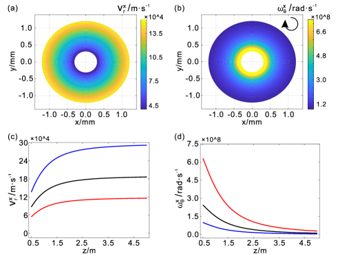
Figure 1: The velocity of a single-mode LG beam in $x$-Bohm theory with $l_{1}=3$ and $a_{1}=1$. (a) and (b) show the radial velocity and angular velocity in the $z=0.5$ m plane, respectively. At each point, the direction of angular velocity is the same, as indicated in the upper right corner of (b). (c) and (d) show how the radial velocity and angular velocity change with the propagation distance, respectively.

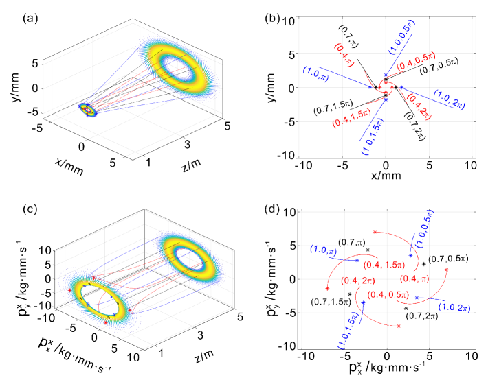
Figure 2: The trajectory of a single-mode LG beam in $x$-Bohm theory with $l_{1}=3$ and $a_{1}=1$. (a) shows the three-dimensional position trajectory of the LG beam from $z=0.5$ m to $z=5$ m. (b) shows the projection of (a) on the xoy plane. (c) shows the three-dimensional momentum trajectory of the LG beam from $z=0.5$ m to $z=5$ m. (d) shows the projection of (c) on the xoy plane. $*$ remarks the starting point. Lines are labeled by initial polar coordinates.

First, we investigate the trajectory of a single-mode LG beam in $x$-Bohm theory with $l_{1}=3$ and $a_{1}=1$. Fig. 1(a) and Fig. 1(b) show the radial velocity and angular velocity of the LG beam in the $z=0.5$ m plane. It can be seen that both velocities depend only on the off-axial distance (i.e., radius); with the distance decreasing, the radial velocity decreases, while the angular velocity increases. This implies that the closer to the center of the LG beam, the slower the divergence and the faster the rotation. Additionally, as depicted in Fig. 1(c) and Fig. 1(d), both velocities change quickly in the near field and become constant in the far field. With the help of Eqs. (3) and (5), we can further derive the three-dimensional position trajectory. Four starting positions are chosen at each radius, and their corresponding three-dimensional position trajectories from $z=0.5$ m to $z=5$ m are shown in Fig. 2(a). Obviously, the rotation velocity of the trajectory decreases as the propagation distance increases. And, inner trajectories (red curves) exhibit faster rotation and slower divergence, while outer trajectories (blue curves) show the opposite trend, consistent with the observed changes in velocity. See Fig. 2(b), the top view of Fig. 2(a) for more clarity. It should be noted that the observed divergence and rotation will induce a reduction in the longitudinal propagation velocity. Consequently, in the communication task, information embedded in LG beams with different initial off-axial distances and propagation distances does not arrive simultaneously, necessitating corrections [27, 28].

By tracking the momentum of each position, the corresponding momentum trajectory can be obtained, as illustrated in Fig. 2(c) and Fig. 2(d). While the intensity distribution of the LG beam in momentum space retains a ring-shaped pattern without significant expansion, the momentum trajectories are not flat lines, excluding those starting at peak intensity (black markers). For trajectories starting within the peak intensity, the radial velocity is positive, and the angular velocity is negative, leading to inward convergence and clockwise rotation. Conversely, for trajectories starting outside the peak intensity, the radial velocity is negative, and the angular velocity is positive, resulting in outward divergence and counter-clockwise rotation. Counter-intuitively, these trajectories “intersect" each other during propagation.

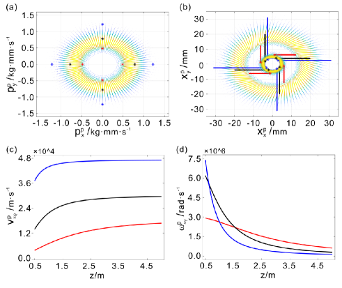
Figure 3: The results of a single-mode LG beam in $p$-Bohm theory with $l_{1}=3$ and $a_{1}=1$. (a) and (b) respectively show the projections of the three-dimensional momentum and position trajectories in the $z=0.5$ m plane. The background density plots in (a) and (b) represent the intensity distribution in the respective planes. (c) and (d) show how the radial velocity and angular velocity change with the propagation distance, respectively. In (a)-(d), lines with the same color have the same radial coordinate.

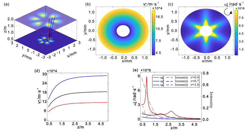
Figure 4: The results of the superposed-mode LG beam in $x$-Bohm theory with $l_{1}=-l_{2}=3$ and (a) $a_{1}=a_{2}=1/\sqrt{2}$, (b-e) $a_{1}=1/\sqrt{10}$, $a_{2}=3/\sqrt{10}$. (a) shows the three-dimensional position trajectory from $z=0.5$ m to $z=2$ m. (b) and (c) show the radial velocity and angular velocity distributions in the $z=0.5$ m plane, respectively. At each point, the direction of angular velocity is the same, as indicated in the upper right corner of (c). (d) and (e) show how the radial velocity and angular velocity change with the propagation distance, respectively. In (a) and (d)-(e), lines with the same color have the same radial coordinate. The background density plots in (a) represents the intensity distribution in the respective plane.

On the other hand, for the freely propagating LG beam, its intensity distribution in momentum space remains constant. Consequently, both the radial velocity $v_{\rho}^{p}$ and angular velocity $\omega_{\varphi}^{p}$ are equal to zero during the propagation. The momentum trajectories in $p$-Bohm theory are represented by straight lines, specifically given by $\rho=\rho_{0}$ and $\varphi=\varphi_{0}$ (see Fig. 3(a)). In contrast to the results depicted in Fig. 2(c) and Fig. 2(d), these trajectories exhibit no divergence and rotation. By tracking each position along the momentum trajectory, the corresponding position trajectory can be obtained, as shown in Fig. 3(b). Surprisingly, these $p$-Bohm position trajectories originate from positions with vanishingly low probabilities according to $x$-Bohm. Notably, in $p$-Bohm theory, position trajectories with the same initial angular coordinate divergence in parallel. This divergence arises from the fact that, while the radial velocity in the $p$-Bohm theory undergoes a similar evolution to that in the $x$-Bohm theory, the angular velocity, particularly in the near field, follows a different trend, being inversely proportional to the radius. See Fig. 3(c) and (d) for more clarity.

4.2 The results for superposed-mode LG beams

In this section, we consider the case when $a_{2}\neq 0$, which indicates the beam is in a superposition state of two LG beams with different $l_{1}$ and $l_{2}$. The intensity distribution of the superposed-mode LG beam is petal-shaped, with the number of petals being $|l_{2}-l_{1}|$. It is straightforward to deduce from Eq. (15) that when $l_{1}=-l_{2}$ and $a_{1}=a_{2}$, the angular velocity becomes zero. As shown in Fig. 4(a), the superposed-mode LG beam exhibits rotation-free propagation, yielding seemingly trivial characteristics.

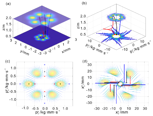
Figure 5: The trajectory of the superposed-mode LG beam with $l_{1}=-l_{2}=3$ and $a_{1}=1/\sqrt{10}$, $a_{2}=3/\sqrt{10}$. (a) and (b) show the three-dimensional position and momentum trajectory of the LG beam from $z=0.5$ m to $z=2$ m in $x$-Bohm theory, respectively. The momentum trajectory and position trajectory of the superposed-mode LG beam in $p$-Bohm theory are shown in (c) and (d), respectively. In (a-d), lines with the same color have the same radial coordinate. The background density plots in (a-d) represents the intensity distribution in the respective plane.

To better illustrate the distinction between superposed-mode and single-model LG beams, we set $l_{1}=-l_{2}=3$, $a_{1}=1/\sqrt{10}$ and $a_{2}=3/\sqrt{10}$ to investigate the propagation characteristics of the superposed-mode LG beam. The corresponding results in $x$-Bohm theory are presented in Fig. 4(b-e) and Fig. 5(a-b) . As shown in Fig. 4(b) and Fig. 4(d), the change in the radial velocity is similar to that of a single-mode LG beam. However, due to interference, the angular velocity exhibits periodic oscillation. Fig. 4(c) and Fig. 4(e) show that in regions with lower angular velocity, trajectories converge together, forming bright petals; conversely, in regions with higher angular velocity, trajectories disperse and form dark petals. After integrating the velocity, the $x$-Bohm position trajectory can be obtained. Fig. 5(a) clearly shows that the inner trajectory moves from one bright petal to another. Furthermore, by tracking the momentum at each point on this trajectory, the momentum trajectory in $x$-Bohm theory can be determined. As shown in Fig. 5(b), the radial velocity in non-primary space is not always positive, especially for the inner trajectory indicated by the red line. Comparing Fig. 5(a) and Fig. 5(b), a distinctive observation emerges: while primary space consistently maintains a perfect petal-shaped intensity distribution, non-primary space can only achieve it in the far field. In $p$-Bohm theory, the petal-shaped intensity distribution remains unchanged in the primary space. However, in the non-primary space, it diverges with the increase of the propagation distance. Interestingly, the evolutions of the $p$-Bohm momentum and position trajectories are similar to those of the single-mode LG beam, yet they deviate from the trajectory observed in $x$-Bohm theory. See Fig. 3(a-b), Fig. 5(a-b), and Fig. 5(c-d) for more clarity.

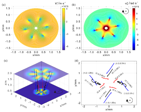
Figure 6: The results of superposed-mode LG beam in the $x$-Bohm theory with $l_{1}=-1$, $l_{2}=5$ and $a_{1}=a_{2}=1/\sqrt{2}$. (a) and (b) show the radial velocity and angular velocity in the $z=0.5$ m plane. (c) shows the three-dimensional position trajectories from $z=0.5$ m to $z=2$ m. Red and blue trajectories respectively start at the extreme intensity of the single-mode LG beam with $l_{1}=-1$ and $l_{1}=5$, while black trajectories start at that of their superposition. The background density plots represent the intensity distribution in the respective planes. (d) shows the projection of (c) on the xoy plane. $*$ remarks the starting point.

The analysis above highlights that the $x$-Bohm theory offers a more familiar dynamical scenario. To comprehensively investigate the propagation characteristics of superposed-mode LG beams, we further explore the dynamic behaviour of LG beam with $l_{1}=-1$, $l_{2}=5$ and $a_{1}=a_{2}=1/\sqrt{2}$ within the framework of $x$-Bohm theory. Fig. 6(a) and Fig. 6(b) show that both the radial velocity and angular velocity change direction around the center of the the dark intensity patterns. The three-dimensional position trajectories from $z=0.5$ m to $z=2$ m are shown in Fig. 6(c). The red and blue trajectories respectively start at the extreme intensity of the single-mode LG beam with $l_{1}=-1$ and $l_{1}=5$, while the black trajectories start at that of their superposition. Obviously, the red trajectory rotates in the opposite direction as the superposed-mode LG beam, while both the blue and black trajectories rotate in the same direction. Additionally, the black trajectory, starting from the minimum intensity, rotates the most quickly. See Fig. 6(d), the top view of Fig. 6(c) for more clarity.

5 Conclusions and Discussion

In this work, we construct the three-dimensional trajectory of LG beams employing the $x$-Bohm theory and $p$-Bohm theory. Our results reveal that the divergence of a single-mode LG beam increases with both off-axis distance and propagation distance, while the rotation behavior displays a distinct dynamic. We rigorously quantify the divergence velocity and rotation velocity, allowing precise adjustment of the arrival time of encoded information in LG beams, which is crucial for communication tasks. Additionally, we find that the distinctive petal-shaped intensity distribution in the superposed-mode LG beam emerges as the trajectories converge when approaching the maximum intensity and diverge on coming out of it. That is why the energy concentrates in the “rear" and dissipates near the “front" of the bright petal. Of course, all these processes can be described in the optical wave language which is used in the original works, but the employment of the propagation trajectory makes the behavior physically clear. In addition, when the absolute values of the angular momentum indices in the superposed-mode LG beam are different, the divergence and rotation direction of the trajectory do not always align with that of the intensity distribution. Instead, they depend on the initial position and propagation distance. Intriguingly, discrepancies are observed between the position and momentum trajectories in $x$-Bohm theory and their counterparts in $p$-Bohm theory. This reveals an asymmetry between position and momentum and underscores the importance of selecting a primary ontological variable [39].

Funding This work was supported by the Fundamental Research Funds for the Central Universities (Grant No. 202364008), the Natural Science Foundation of Shandong Province of China (Grant No. ZR2021ZD19), and the Young Talents Project at Ocean University of China (Grant No. 861901013107).

Data availability The data sets generated during and/or analyzed during the current study are available from the corresponding author on reasonable request.

Disclosures The authors have no competing interests to declare that are relevant to the content of this article.

Disclosures The authors promise that the results of this article are correct and original and it has not been published in other journals before.

References

- [1] L. Allen, M. W. Beijersbergen, R. J. C. Spreeuw, et al., “Orbital angular momentum of light and the transformation of Laguerre-Gaussian laser mode,” Phys. Rev. A 45, 8185 (1992).
- [2] A. E. Willner, K. Pang, H. Song, et al., “Orbital angular momentum of light for communication,” Appl. Phys. Rev. 8, 041312 (2021).
- [3] A. E. Willner, H. Huang, Y. Yan, et al., “Optical communications using orbital angular momentum beams,” Adv. Opt. Photon. 7, 66 (2015).
- [4] N. Bozinovic, Y. Yue, Y. Ren, et al., “Terabit-scale orbital angular momentum mode division multiplexing in fibers,” Science 340, 1545 (2013).
- [5] M. Padgett and R. Bowman, “Tweezers with a twist,” Nat. Photonics 5, 343 (2011).
- [6] E. Otte, and C. Denz, “Optical trapping gets structure: structured light for advanced optical manipulation,” Appl. Phys. Rev. 7, 041308 (2020).
- [7] L. Gong, B. Gu, G. Rui, et al., “Optical forces of focused femtosecond laser pulses on nonlinear optical Rayleigh particles,” Photonics Res. 6, 138 (2018).
- [8] Z. Shi, Z. Wan, Z. Zhan, et al., “Super-resolution orbital angular momentum holography,” Nat. Commun. 14, 1869 (2023).
- [9] Z. Wu, R. Gao, S. Zhou, et al., “Robust super-resolution image transmission based on a ring core fiber with orbital angular momentum,” Laser Photonics Rev., 2300624 (2023).
- [10] Y. Kozawa, D. Matsunaga, and S. Sato, “Superresolution imaging via super-oscillation focusing of a radially polarized beam,” Optica 5, 86 (2018).
- [11] J. Pinnell, I. Nape, M. de Oliveira, et al., “Experimental demonstration of 11-dimensional 10-party quantum secret sharing,” Laser Photonics Rev. 14, 2000012 (2020).
- [12] L.-J. Kong, Y. Sun, F. Zhang, et al., “High-Dimensional Entanglement-Enabled Holography,” Phys. Rev. Lett. 130, 053602 (2023).
- [13] X.-L. Wang, X.-D. Cai, Z.-E. Su, et al., “Quantum teleportation of multiple degrees of freedom of a single photon,” Nature(London) 518, 516 (2015).
- [14] X. Fang, H. Ren, and M. Gu, “Orbital angular momentum holography for high-security encryption,” Nat. Photonics 14, 102 (2020).
- [15] C. He, Y.-J. Shen, and A. Forbes, “Towards higher-dimensional structured light,” Light. Sci. Appl. 11, 205 (2022).
- [16] M. P. J. Lavery, F. C. Speirits, S. M. Barnett, et al., “Detection of a spinning object using light’s orbital angular momentum,” Science 341, 537 (2013).
- [17] N. Uribe-Patarroyo, A. Fraine, D. S. Simon, et al., “Object identification using correlated orbital angular momentum states,” Phys. Rev. Lett. 110, 043601 (2013).
- [18] K. Zhang, Y. Wang, Y. Yuan, et al., “A review of orbital angular momentum bortex beams generation: from traditional methods to metasurfaces,” Appl. Sci. 10, 1015 (2020).
- [19] Y. Lian, X. Qi, Y. Wang, et al., “OAM beam generation in space and its applications: a review,” Opt. Lasers Eng. 151, 106923 (2022).
- [20] J. Wang, and Y. Liang, “Generation and detection of structured light: a review,” Front. Phys. 9, 688284 (2021).
- [21] Y. Xiao, H. Liu, Y. Song, et al., “Accurately quantifying the superposition state of two different Laguerre-Gaussian modes with single intensity distribution measurement,” Quantum Inf. Process 21, 90 (2022).
- [22] J. Zhu, P. Zhang, F. Wang, et al., “Experimentally measuring the mode indices of Laguerre-Gaussian beams by weak measurement,” Opt. Express 29, 5419 (2021).
- [23] T. Doster, and A. T. Watnik, “Machine learning approach to oam beam demultiplexing via convolutional neural networks,” Appl. Opt. 56, 3386 (2017).
- [24] X. Yin, X. Cui, H. Chang, et al., “Research progress of orbital angular momentum modes detecting technology based on machine learning,” Opto-Electron Eng. 47, 190584 (2020).
- [25] Y. Li, Z. Ren, L. Kong, et al., “Trajectory-based unveiling of the angular momentum of photons,” Phys. Rev. A 95, 043830 (2017).
- [26] M. Cai, Q. Wang, Y. Li, et al., “Propagation and focusing properties of vortex beams based on light ray tracing,” Front. Phys. 10, 931131 (2022).
- [27] F. Bouchard, J. Harris, H. Mand, et al., “Observation of subluminal twisted light in vacuum,” Optica 3, 351 (2016).
- [28] A. Lyons, T. Roger, N. Westerberg, et al., “How fast is a twisted photon?” Optica 5, 682 (2018).
- [29] W. Heisenberg, “Über den anschaulichen inhalt der quantentheoretischen kinematik und mechanik,” Z. Phys. 43, 172 (1927).
- [30] D. Bohm, “A suggested interpretation of the quantum theory in terms of "hidden" variables. I,” Phys. Rev. 85, 166 (1952).
- [31] D. Bohm, “A suggested interpretation of the quantum theory in terms of "hidden" variables. II,” Phys. Rev. 85, 180 (1952).
- [32] S. T. Epstein, “The causal interpretation of quantum mechanics,” Phys. Rev. 89, 319 (1953).
- [33] S. T. Epstein, “The causal interpretation of quantum mechanics,” Phys. Rev. 91, 985 (1953).
- [34] H. M. Wiseman, “Grounding Bohmian mechanics in weak values and bayesianism,” New J. Phys. 9, 165 (2007).
- [35] S. Kocsis, B. Braverman, S. Ravets, et al., “Observing the average trajectories of single photons in a two-slit interferometer,” Science 332, 1170 (2011).
- [36] D. H. Mahler, L. Rozema, K. Fisher, et al., “Experimental nonlocal and surreal Bohmian trajectories,” Sci. Adv. 2, 1501466 (2016).
- [37] Y. Xiao, Y. Kedem, J.-S. Xu, et al., “Experimental nonlocal steering of Bohmian trajectories,” Opt. Express 25, 14463 (2017).
- [38] Y. Xiao, H. M. Wiseman, J.-S. Xu, et al., “Observing momentum disturbance in double-slit “which-way" measurements,” Sci. Adv. 5, aav9547 (2019).
- [39] A. O. T. Pang, H. Ferretti, N. Lupu-Gladstein, et al., “Experimental comparison of Bohm-like theories with different ontologies,” Quantum 4, 365 (2020).
- [40] M. Yang, Y. Xiao, Y.-W. Liao, et al., “Zonal reconstruction of photonic wavefunction via momentum weak measurement,” Laser Photonics Rev. 14, 1900251 (2020).
- [41] The corresponding codes for reconstructing the propagation trajectories of Laguerre-Gaussian beams using -Bohm theory and -Bohm theory can be found at: https://github.com/Hpf-77/LG-trajectory.git