Intent Prediction-Driven Model Predictive Control for UAV Planning and Navigation in Dynamic Environments

Abstract

The emergence of indoor aerial robots holds significant potential for enhancing construction site workers' productivity by autonomously performing inspection and mapping tasks. The key challenge to this application is ensuring navigation safety with human workers. While navigation in static environments has been extensively studied, navigating dynamic environments remains open due to challenges in perception and planning. Payload limitations of unmanned aerial vehicles limit them to using cameras with limited fields of view, resulting in unreliable perception and tracking during collision avoidance. Moreover, the unpredictable nature of the dynamic environments can quickly make the generated optimal trajectory outdated. To address these challenges, this paper presents a comprehensive navigation framework that incorporates both perception and planning, introducing the concept of dynamic obstacle intent prediction. Our perception module detects and tracks dynamic obstacles efficiently and handles tracking loss and occlusion during collision avoidance. The proposed intent prediction module employs a Markov Decision Process (MDP) to forecast potential actions of dynamic obstacles with the possible future trajectories. Finally, a novel intent-based planning algorithm, leveraging model predictive control (MPC), is applied to generate safe navigation trajectories. Simulation and physical experiments demonstrate that our method enables safe navigation in dynamic environments and achieves the fewest collisions compared to benchmarks.

I Introduction

In recent years, lightweight autonomous unmanned aerial vehicles (UAVs) have shown great potential for inspection and mapping in indoor construction sites [1][2][3]. Unlike the open outdoor environments, indoor construction sites present more complex conditions, including the presence of moving workers, machines, and other static structures in close proximity. Ensuring the operational safety of these autonomous robots in relation to human workers is thus a critical challenge that must be addressed before their deployment. As a result, designing a navigation framework that enables safe operation in dynamic environments is essential.

Despite the success of previous research [4][5] in navigation for complex static environments, achieving safe robot navigation in dynamic environments remains challenging due to two major factors. First, the low image quality of onboard cameras in lightweight UAVs makes accurate detection and tracking of dynamic obstacles difficult. Although our previous work [6] utilizes an ensemble detection method to improve accuracy and computational efficiency, the camera's limited field of view (FOV) can still result in tracking failures during collision avoidance maneuvers, increasing the risk of severe collisions from undetected dynamic obstacles. Second, the unpredictable motion of dynamic obstacles can quickly make an optimized trajectory ineffective. While many previous works [7][8][9][10] have incorporated obstacle trajectory prediction into planning frameworks, most methods consider only a single future mode (i.e., one trajectory) per obstacle, typically using a simple linear motion model. Although these approaches can improve dynamic obstacle avoidance, their effectiveness is significantly diminished if the actual motion of the obstacles differs from the assumed model.

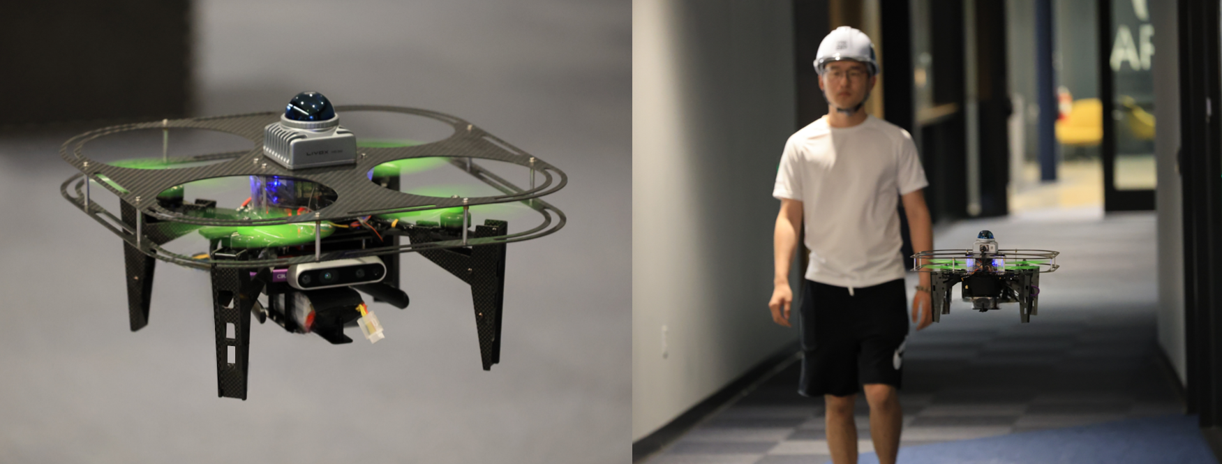
Figure 1: The UAV navigating a dynamic environment using the proposed algorithm. The left figure shows our customized UAV equipped with onboard sensors and the right figure illustrates the UAV avoiding a pedestrian.

To address these challenges, this paper presents an intent prediction-driven and comprehensive navigation framework based on a model predictive control scheme. An enhanced perception module for dynamic obstacle detection and tracking is introduced to mitigate the lost-tracking issue during collision avoidance maneuvers. Crucially, to enable the planner to consider all potential future movements of dynamic obstacles, this work introduces the concept of dynamic obstacle intents, represented as a probability distribution that reflects the likelihood of predefined high-level decisions for each obstacle. Instead of predicting a single trajectory per obstacle, the prediction module generates all possible trajectories based on various possible intents. The proposed trajectory planning algorithm optimizes multiple trajectories according to potential future states using model predictive control formulation and applies a scoring function to select the best trajectory for execution. Fig. 1 shows an example of our UAV navigating in a dynamic environment with the proposed method. The contributions of this work are:

• Lost-Tracking-Aware Perception: Building on previous work in obstacle detection and tracking [6], the perception module is enhanced with an out-of-view compensation method to mitigate lost tracking and occlusion during collision avoidance maneuvers.

• Intent and Trajectory Prediction: This work introduces dynamic obstacle intent prediction, which forecasts potential actions and future trajectories using a Markov Decision Process, enabling more comprehensive anticipation of movements within the environment.

• Intent-Based Planning Algorithm: Unlike traditional methods optimizing a single trajectory based on one future prediction per obstacle, our algorithm generates multiple candidates and selects the highest-score one by evaluating potential future states, thereby reducing trajectory flickering in unpredictable environments.

II Related Work

Recent years have seen significant advances in lightweight indoor UAV navigation. While early challenges in trajectory planning [11][12] and collision avoidance [13][14] for static environments have been largely addressed [4][5][15], navigating dynamic environments remains a challenge due to the unpredictable nature of dynamic obstacles. Research efforts to improve UAV navigation safety and efficiency in dynamic environments can be broadly categorized into reactive planning-based and predictive planning-based methods.

Reactive planning-based methods: These methods treat dynamic obstacles as static at each time step, adapting static planning methods to dynamic environments through high-frequency replanning. Oleynikova et al. [16] use depth vision to detect obstacles and generate waypoints for collision avoidance. In [4][5], occupancy-based maps are adopted for environment representation, which enables safe trajectory generation. Similarly, Ren et al. [15] achieve aggressive and safe maneuvering using whole-body motion planning. However, because these methods are primarily designed for static obstacles, their lack of dynamic obstacle perception and planning can lead to potential failures. To address the future uncertainties of dynamic obstacles, Guo et al. [17] construct risk regions, while [18] adopts a safe flight corridor that considers both static and dynamic obstacles. In [19], moving obstacle avoidance is achieved through raycasting and Riemannian motion policy. Although some reactive methods can achieve safe navigation, they can become significantly less effective and risky in highly dynamic environments.

Predictive planning-based methods: Different from the reactive methods, methods from this category make plans utilizing the prediction of dynamic obstacles in a future horizon. In [20][7][21], a chance-constrained model predictive control approach is used to account for the uncertainties of dynamic obstacles. Similarly, Jian et al. [22] employ a control barrier function within an MPC framework for collision avoidance. Wang et al. [8] enhance safe navigation by combining occlusion-aware obstacle tracking with spline-based trajectory optimization. Chen et al. [23] sample and evaluate trajectories based on predicted dynamic obstacles, while [10] incorporates UAV yaw angle for collision avoidance. In [9], a vision-aided planner is used for avoiding both static and dynamic obstacles. For dynamic obstacle perception, a learning-based method [24] is proposed for 3D detection and tracking, with further improvements in computation and accuracy achieved through ensemble detection in [6]. Additionally, some methods [25][26] use learning-based approaches to avoid dynamic obstacles. However, these methods only rely on a constant velocity model for predicting the future state of dynamic obstacles, which may not always be reliable. To better model pedestrian trajectories, Peddi et al. [27] trained a Hidden Markov Model on trajectory datasets, and Thomas et al. [28] applied self-supervised learning for map-level dynamic obstacle prediction. Although these methods, along with other popular learning-based approaches [29][30], improve upon traditional linear predictions, they primarily focus on low-level trajectory prediction and fail to account for the high-level decision-making processes of dynamic obstacles, potentially overlooking variations in obstacle behavior. Inspired by methods in autonomous driving [31][32][33][34] that predict multiple future trajectories for vehicles, we introduce the concept of dynamic obstacle intent. Our approach considers the high-level decisions of obstacles, predicts trajectories based on these intents, and generates safe trajectories accordingly.

III Methodology

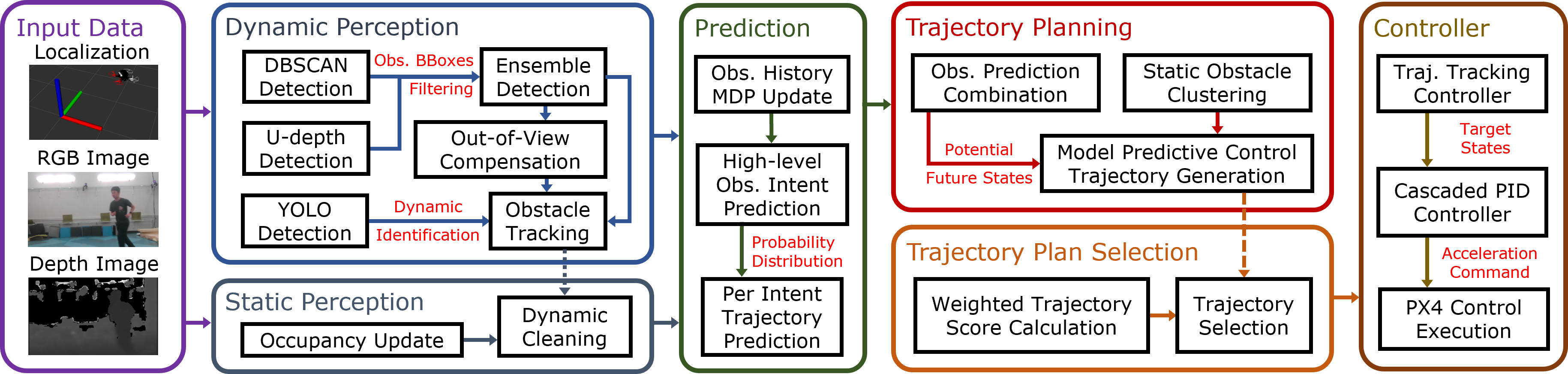
Figure 2: The proposed dynamic environment navigation system framework. Given localization, RGB, and depth image data, the static perception module constructs an occupancy map, while the dynamic perception module detects and tracks dynamic obstacles with out-of-view compensation. With the tracked obstacles' histories, the prediction module anticipates future obstacle trajectories using intent prediction. The intent-based planning algorithm, including trajectory planning and selection, then optimizes and selects the highest-score trajectory. Finally, the selected trajectory is sent to the controller for execution.

The proposed method contains three main modules: perception, prediction, and planning, as shown in Fig. 2. The perception module (Sec. III-A) is divided into two parts, handling static and dynamic obstacle perception, respectively. The intent and trajectory prediction module (Sec. III-B) processes dynamic obstacle history from the dynamic perception module and the occupancy map from the static perception module to generate intent probability distributions and corresponding predicted trajectories for dynamic obstacles. The intent-based planning algorithm (Sec. III-D) includes a trajectory planning that uses a model predictive control formulation (Sec. III-C) and a score-based trajectory selection module to produce the final trajectory for execution.

III-A Lost-Tracking-Aware Perception

The perception module consists of a static and a dynamic component for separate obstacle detection. As shown in Fig. 2, the static perception uses a traditional occupancy voxel map to represent static obstacles, with dynamic cleaning to remove noise caused by moving obstacles. The dynamic perception is based on [6] and incorporates an updated ensemble detection method along with out-of-view compensation to improve accuracy and safety during collision avoidance, particularly in dynamic-obstacle-tracking loss scenarios.

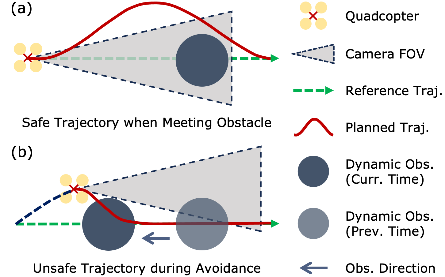
Figure 3: Illustration of unsafe dynamic obstacle avoidance due to tracking loss. (a) The robot initially detects and tracks the dynamic obstacle, generating a safe trajectory. (b) As the robot maneuvers, the obstacle moves out of the camera view, leading to an unsafe replanned trajectory.

Dynamic Obstacle Detection: The main challenge in 3D dynamic obstacle detection arises from the noisy depth images captured by lightweight UAV cameras, and the limited processing power of the UAV's onboard computer makes computationally intensive methods like [35] impractical. To achieve high-accuracy results while maintaining the computational cost manageable, we propose an ensemble detection method that integrates two lightweight detectors. The first, known as the DBSCAN detector, uses the DBSCAN clustering algorithm on point cloud data from depth images to determine obstacle centers and sizes based on the boundary points in each cluster. The second, the U-depth detector, processes raw depth images to create a U-depth map (similar to a top-down view) and uses a contiguous line-grouping algorithm [16][7] to detect 3D bounding boxes of obstacles. Note that, due to the noisy input data, both detectors can produce a significant number of false-positive results. The proposed ensemble detection method addresses this issue by identifying the mutual agreements between the two detectors. In addition, since the detection results may include both static and dynamic obstacles, a lightweight YOLO detector is applied to the re-projected 2D bounding boxes in the image plane from the 3D results to classify dynamic obstacles.

Feature-based Tracking: With the detected obstacles, feature-based tracking is used to estimate their states (i.e., positions and velocities). To minimize detection mismatches over time that can occur with the closest-center-point association method, a feature-based association method is proposed. The feature vector of an obstacle $\text{o}_{i}$ is defined as:

$$f(\text{o}_{i})=[\text{pos}(\text{o}_{i}),\ \text{dim}(\text{o}_{i}),\ \text{len}(\text{o}_{i}),\ \text{std}(\text{o}_{i})]^{T},$$ (1)

which includes information about the obstacle's position, dimensions, and the length and standard deviation of the point cloud. To associate obstacles between the current and previous time steps, the two detected obstacles, $\text{o}_{i}$ and $\text{o}_{j}$, with the highest similarity score are selected, calculated as:

$$\text{sim}(\text{o}_{i},\text{o}_{j})=\text{exp}(-||W(f(\text{o}_{i})-f(\text{o}_{j}))||_{2}^{2}),$$ (2)

where $W$ is a diagonal matrix that weights the obstacle features. After the association process is complete, a linear Kalman filter with a constant acceleration model is applied to estimate the positions and velocities of the obstacles.

Out-of-View Compensation: Unlike stationary sensors, the onboard camera moves with the robot during collision avoidance maneuvers. As shown in Fig. 3a, the robot may initially generate a safe trajectory with the obstacle entirely within the camera's field of view. However, Fig. 3b illustrates that the replanned trajectory can become unsafe if the obstacle moves out of view during the maneuver. To address this issue, out-of-view compensation is introduced to estimate the states of obstacles when tracking is lost. Whenever a previously tracked dynamic obstacle moves out of view, instead of completely ignoring the obstacle, its position is linearly extrapolated using its estimated velocity, and its size is gradually inflated to account for uncertainties over a short time horizon. In our experiments, this out-of-view compensation significantly improves trajectory safety.

III-B Intent and Trajectory Prediction

The prediction module, which activates after the perception, contains two steps: the high-level intent prediction and the trajectory-level prediction. The proposed method forecasts the potential high-level actions of dynamic obstacles and then performs the trajectory prediction step to generate possible future states for all intents (Fig. 4a). This process is crucial for comprehensively anticipating the behaviors of dynamic obstacles and generating safe trajectories.

Intent Prediction: The various obstacle intents represent different high-level decisions of the dynamic obstacle. To model the changes in these decisions over time, we apply a Markov Decision Process (MDP), where the intents serve as the MDP states. The intent $\mathbb{I}^{\text{o}_{i}}_{t}$ of the $i$-th dynamic obstacle at time $t$ can be selected from a finite set $\mathcal{I}$ defined as:

$$\mathcal{I}=\{\text{forward},\text{left},\text{right},\text{stop}\},\ \mathbb{I}^{\text{o}_{i}}_{t}\in\mathcal{I}.$$ (3)

Here we define four intents to consider the forwarding, turning, and stopping decisions of dynamic obstacles. Based on the historical trajectory of the $i$-th dynamic obstacle, our goal is to estimate the probability distribution $P^{o_{i}}_{\mathcal{T}}(\mathcal{I})$ over the set of possible intents at the current time $\mathcal{T}$. Note that dynamic obstacles are assumed to move in the 2D plane.

We begin by computing the raw intent probability $\tilde{P}^{o_{i}}_{t}(\mathcal{I})$, which represents the intent probability distribution considering only the obstacle states at the time $t$ and the previous time step $t-1$. Given the obstacle states, the motion angle $\theta_{t}$ is defined as the angle between the obstacle current velocity $v_{t}$ and its facing direction vector $f_{t}=p_{t}-p_{t-1}$. For clarity, we omit the superscript for obstacle $o_{i}$ and use $p_{t}$ to represent obstacle position at time $t$. Consequently, the raw intent probability distribution $\tilde{P}^{o_{i}}_{t}$ can be computed as follows:

$$\begin{split}\tilde{P}^{o_{i}}_{t}(\mathcal{I})=\frac{\hat{P}^{o_{i}}_{t}(\mathcal{I})}{\lVert\hat{P}^{o_{i}}_{t}(\mathcal{I})\lVert},\ \text{where}\ \hat{P}^{o_{i}}_{t}(\mathcal{I})=[e^{-\alpha\theta_{t}^{2}},...\\ \ \beta(1+\sin{\theta_{t}}),\ \beta(1-\sin{\theta_{t}}),\ 1-\tanh{(\gamma\lVert v_{t}\rVert})]^{T},\end{split}$$ (4)

where the values of the raw intent probability distribution is calculated based on the order of the intent set $\mathcal{I}$, with $\alpha,\beta,\gamma$ being user-defined parameters that control the probability balance across various intents. The underlying intuition is that as the motion angle goes close to zero, the probability of the forward intent increases relative to the turning intents. Similarly, when the obstacle's speed is low, the probability of the stopping intent increases compared to the other intents.

To fully leverage the trajectory of the dynamic obstacle, we use the raw intent probability $\tilde{P}^{o_{i}}_{t}$ to first construct the unnormalized transition matrix $\hat{T}^{o_{i}}_{t}$ of the MDP at time $t$:

$$\hat{T}^{o_{i}}_{t}=\Sigma_{t}\cdot(\tilde{P}^{o_{i}}_{t}(\mathcal{I})\otimes\textbf{1}^{T}),\ \ \Sigma_{t}\in\mathbb{R}^{4\times 4},$$ (5)

where $(\cdot\otimes\textbf{1}^{T})$ represents the operation of expanding a vector into a square matrix, and $\Sigma_{t}$ is a diagonal matrix with all entries equal to one, except for the $n$-th entry, which is set to $s(s>1)$ corresponding to the previous intent index with the highest probability. This setup of $\Sigma_{t}$ reflects the obstacle's tendency to continue with its previous intent. The transition matrix $T^{o_{i}}_{t}$ is then obtained by normalizing each row of $\hat{T}^{o_{i}}_{t}$.

Finally, by initializing the intent probability $P^{o_{i}}_{0}$ at $t=0$ to a uniform distribution, we can apply the MDP to obtain the intent probability distribution $P^{o_{i}}_{\mathcal{T}}$ at current time $\mathcal{T}$ using:

$$P^{o_{i}}_{\mathcal{T}}=(\prod_{t=0}^{\mathcal{T}}T^{o_{i}}_{t})\cdot P^{o_{i}}_{0},\ \text{where}\ \mathcal{T}=n\Delta t.$$ (6)

This process is computed at each time step with only a limited duration of each dynamic obstacle's history retained. The computed intent probability distribution is utilized by the planning algorithm, which will be discussed in later sections.

Trajectory Prediction: The trajectory-level prediction computes the future positions and risk sizes of the obstacle for all possible intents, as outlined in Alg. 1. It is important to note that for each obstacle, trajectories are predicted for all four intents, regardless of the intent probability distribution. For the stop intent (Lines 1-1), the predicted positions replicate the current obstacle position, while the risk sizes are inflated based on the obstacle's velocity and the time elapsed. For the forward, left, and right intents, a set of control inputs based on the current velocity is first generated (Lines 1-1). Constant linear and angular velocities are then applied to propagate the obstacle positions. The forward intent generates controls by varying the linear velocity within a predefined range while setting the angular velocity to zero (Line 1), whereas the left and right intents adjust both angular and linear velocities within their respective predefined ranges (Line 1). By applying these control combinations to the obstacle (Lines 1-1) with propagation continuing until a collision occurs, multiple trajectories are sampled for each intent. Finally, the predicted trajectory is determined by averaging the positions of all sampled trajectories at each time step, and the risk sizes of the obstacle are inflated by adding a value proportional to the standard deviation of the sampled trajectory positions (Lines 1-1). If the mean trajectory is not collision-free, a sampled trajectory closest to the mean trajectory will be selected. Fig. 4b visualizes the sampled trajectories for the right intent as red dotted curves and the final predicted trajectory as a blue solid curve.

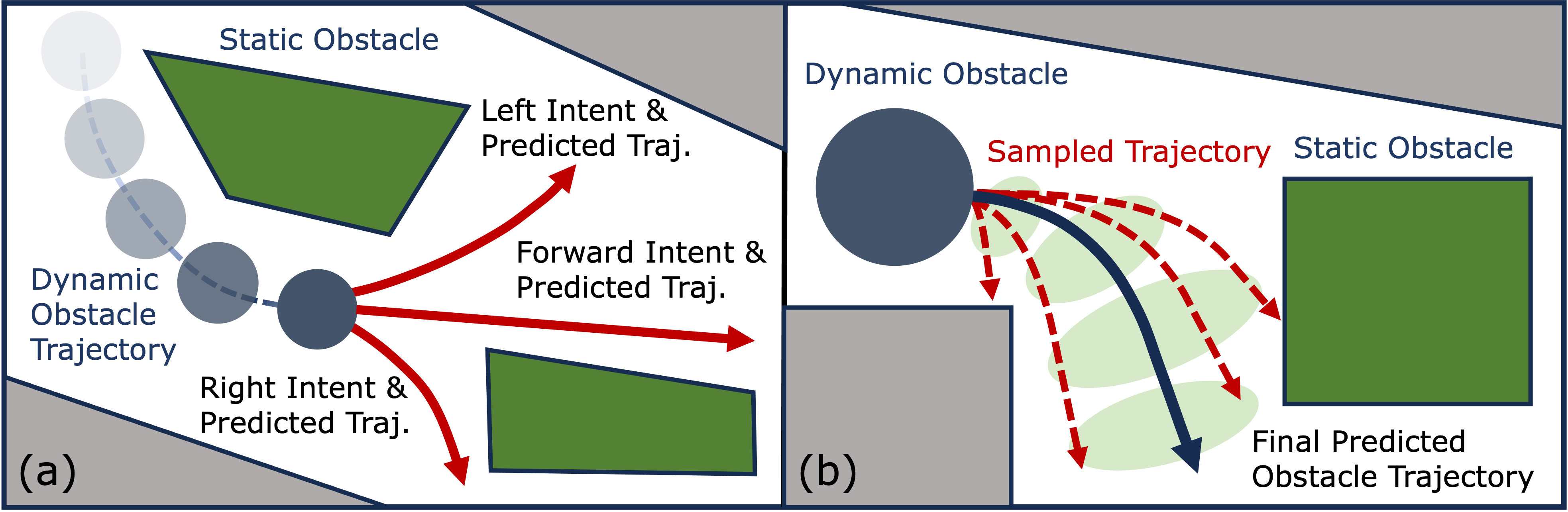
Figure 4: Illustration of the proposed prediction method. (a) Predicted trajectories (red curves) are generated from possible obstacle intents based on the obstacle's historical trajectory and the environment. (b) The example demonstrates trajectory prediction for the obstacle's right (direction) intent. The final predicted trajectories are represented by the mean of the sampled trajectories, with the trajectory variance indicated by shaded green areas.

1 $o\leftarrow\text{Input Dynamic Obstacle}$;

2 $N_{\text{pred}}\leftarrow\text{Prediction Time Steps}$;

$p^{o},v^{o},s^{o}\leftarrow\textbf{obsInfo}(o)$ ;

  $\triangleright$ pos, vel, size

$\text{predictions}\leftarrow\emptyset$ ;

  $\triangleright$ all intent predictions

3 for $\mathbb{I}^{o}$ in $\mathcal{I}$ do

      $\mathcal{P}_{\text{pos}},\mathcal{P}_{\text{size}}\leftarrow\emptyset$ ;

       $\triangleright$ prediction array

4      if $\mathbb{I}^{o}$ is stop then

5           for n in ${\textbf{range}}(0,N_{\text{pred}})$ do

6                $\mathcal{P}_{\text{pos}}.{\textbf{append}}(p^{o})$;

7                $\mathcal{P}_{\text{size}}.{\textbf{append}}(s^{o}+n\Delta t\cdot{\textbf{min}}(v^{o},v_{\text{thresh}}))$;

8               

9                ${\text{predictions}}.{\textbf{append}}(\{\mathcal{P}_{\text{pos}},\mathcal{P}_{\text{size}}\})$;

10                continue;

11               

12                if $\mathbb{I}^{o}$ is forward then

13                     $\mathcal{S}_{\text{control}}\leftarrow{\textbf{getLinearControlSet}}(v^{o})$; 

14                     else if $\mathbb{I}^{o}$ is left or $\mathbb{I}^{o}$ is right then

15                          $\mathcal{S}_{\text{control}}\leftarrow{\textbf{getTurningControlSet}}(v^{o},\mathbb{I}^{o})$; 

                          $\mathcal{S}_{\text{traj}}\leftarrow\emptyset$ ;

                           $\triangleright$ pred trajectory array

16                          for $\text{c}_{i}$ in $\mathcal{S}_{\text{control}}$ do

17                               $\sigma_{\text{traj}}\leftarrow{\textbf{getConstControlTraj}(p^{o},c_{i},N_{\text{pred}}})$;

18                               $\mathcal{S}_{\text{traj}}.{\textbf{append}}(\sigma_{\text{traj}})$;

19                              

20                               $\mathcal{P}_{\text{pos}},\mathcal{V}_{\text{pos}}\leftarrow{\textbf{getPositionMeanAndVar}}(\mathcal{S}_{\text{traj}})$;

21                               $\mathcal{P}_{\text{size}}\leftarrow\lambda\cdot\sqrt{\mathcal{V}_{\text{pos}}}+s^{o}$;

22                               ${\text{predictions}}.{\textbf{append}}(\{\mathcal{P}_{\text{pos}},\mathcal{P}_{\text{size}}\})$;

23                              

24                               return predictions;

Algorithm 1 Trajectory-level Prediction

III-C MPC Formulation for Trajectory Generation

Given an input reference trajectory, we apply the model predictive control method to generate a safe trajectory. The entire optimization problem can be formulated as: [2] x_0:N, u_0:N-1∑_k=0^N ∥xk- xkref∥^2 + ∑_k=0^N-1 λ_u∥uk∥^2, x_0=x(t_0) x_k=f(x_k-1, u_k-1) u_min ≤u_k ≤u_max x_k ／∈C_i, ∀i ∈S^static_o ∪S^dynamic_o ∀k ∈{0, …, N}, where $\mathbf{x}$ and $\mathbf{u}$ represent the robot states and control inputs with the subscript indicating the time step. The objective (Eqn. III-C) is to minimize the distance to the reference trajectory while using the least amount of control effort possible. Eqn. III-C sets the initial state constraint based on the current robot states. The robot's dynamics model and control limits are presented by Eqns. III-C and III-C, respectively.

The collision constraints (Eqn. III-C) ensure that the robot avoids collisions with static and dynamic obstacles. Static obstacles are represented in an occupancy voxel map, while dynamic obstacles are detected as axis-aligned 3D bounding boxes. To simplify the expression of the collision constraints, we unify the representations by converting static obstacles into oriented 3D bounding boxes with a proposed hierarchical clustering method. Initially, surrounding occupancy voxels are collected as a point cloud, and the DBSCAN clustering algorithm is applied as the first level to determine the rough centroid and dimensions of the static obstacles. This step ensures that all static obstacle voxels are enclosed within one of the DBSCAN-clustered bounding boxes, though these boxes may include empty spaces. To refine these DBSCAN-clustered bounding boxes, we then iteratively apply the K-means++ algorithm, starting with two initial centroids at the corners of the bounding boxes and continuing until the point-cloud density within the boxes exceeds a specified threshold. Finally, the 2D orientation angle $\phi$ of each static obstacle bounding box is adjusted in a discretized manner to further maximize point-cloud density. With both static and dynamic obstacles uniformly represented as 3D bounding boxes, the collision constraint for each obstacle can be expressed as:

$$\frac{(x\cos{\phi}+y\sin{\phi})^{2}}{a^{2}}+\frac{(-x\sin{\phi}+y\cos{\phi})^{2}}{b^{2}}+\frac{z^{2}}{c^{2}}\geq 1,$$ (7)

where $a$, $b$, and $c$ are the half-lengths of the principal axes of the minimum ellipsoid enclosing the obstacle's risk-size bounding box, and $x$, $y$, and $z$ are the relative positions along the three axes between the robot and the obstacle centroid.

III-D Intent-Based Trajectory Planning

1 $\mathcal{M}\leftarrow\text{Static Occupancy Map}$;

2 $p^{r}\leftarrow\text{Current Robot Position}$;

3 $\mathbf{\sigma}_{\text{ref}}\leftarrow\text{Input Reference Trajectory}$;

4 $\mathbf{N}_{ic}\leftarrow\text{Number of Intent Combinations}$;

5 $\mathcal{S}_{so}\leftarrow{\textbf{clusterStaticObstacles}}(\mathcal{M},p^{r})$;

6 $\mathcal{S}_{do}\leftarrow{\textbf{closeDynamicObstacles}}(p^{r})$;

7 $\mathcal{S}_{ic}\leftarrow{\textbf{topIntentCombinations}}(\mathcal{S}_{do},N_{ic})$;

8 $\sigma_{\text{output}}\leftarrow\emptyset,\ \text{highestScore}\leftarrow 0$;

9 for $n$ in ${\textbf{range}}(0,N_{ic})$ do

      $\mathcal{IC}\leftarrow\mathcal{S}_{ic}[n]$ ;

       $\triangleright$ Intent Combination

10      $\mathcal{S}^{\text{pred}}_{\text{do}}\leftarrow{\textbf{getObstaclePredictions}}(IC,\mathcal{S}_{do})$;

11      $\sigma_{\text{traj}}\leftarrow{\textbf{MPCTrajGeneration}}(\sigma_{\text{ref}},\mathcal{S}_{so},\mathcal{S}^{\text{pred}}_{do})$;

12      $\text{score}\leftarrow P_{ic}\cdot{\textbf{evaluateTraj}}(\sigma_{\text{traj}})$;

13      if ${\text{score}}>{\text{highestScore}}$ then

14           $\sigma_{\text{output}}\leftarrow\sigma_{\text{traj}}$;

15           $\text{highestScore}\leftarrow\text{score}$;

16          

17          

18           $\textbf{return}\ \sigma_{\text{output}}$;

Algorithm 2 Intent-based Trajectory Planning

With the dynamic obstacle trajectory prediction and MPC formulation introduced, this section presents the intent-based trajectory planning algorithm. The proposed algorithm (Alg. 2) generates multiple trajectories corresponding to different obstacle intent combinations and selects the optimal one for execution based on an evaluation system. Initially, static obstacles are clustered into a set of bounding boxes $\mathcal{S}_{so}$, and the set of risky dynamic obstacles $\mathcal{S}_{do}$ near the robot is identified (Lines 2-2). Next, the top $N_{ic}$ intent combinations $S_{ic}$ for different obstacles are determined based on their current intent probability distributions. Each intent combination, denoted as $\mathcal{IC}$ in Line 2, represents one possible future action scenario for all obstacles, with the algorithm focusing on the most likely $N_{ic}$ scenarios. For a single intent combination, the trajectory-level prediction is obtained for each obstacle (Line 2), and MPC is used to generate a collision-free trajectory $\sigma_{\text{safeTraj}}$ for navigation (Line 2). Finally, the score of the generated trajectory is calculated by combining the intent combination probability $P_{ic}$ with the raw score from the evaluation system (Lines 2-2). The algorithm selects the highest-score trajectory for execution.

The evaluation system computes the raw trajectory score using a weighted sum of three components: the consistency score, the detouring score, and the safety score:

$$\mathbb{S}_{\text{traj}}=\lambda_{\text{1}}\cdot\mathbb{S}_{\text{cons}}+\lambda_{\text{2}}\cdot\mathbb{S}_{\text{detour}}+\lambda_{\text{3}}\cdot\mathbb{S}_{\text{safety}},$$ (8)

where $\lambda_{1}$, $\lambda_{2}$, and $\lambda_{3}$ are user-defined weights. The consistency score evaluates how closely the new trajectory matches the previous one to prevent oscillating behaviors:

$$\mathbb{S}_{\text{cons}}=\frac{N}{\sum_{k=1}^{N}\lVert\sigma_{\text{traj}}(k)-\sigma_{\text{traj}}^{\text{prev}}(k)\rVert}.$$ (9)

Similarly, the detouring score is calculated based on the point-wise distance between the trajectory and the reference:

$$\mathbb{S}_{\text{detour}}=\frac{N}{\sum_{k=1}^{N}\lVert\sigma_{\text{traj}}(k)-\sigma_{\text{ref}}(k)\rVert}.$$ (10)

Both the consistency score and the detouring score are capped at a maximum allowable value to prevent extremely high scores when the denominators approach zero. The safety score is determined by the distance to static and dynamic obstacles under the most likely intent combination:

$$\mathbb{S}_{\text{safety}}=\frac{1}{N}\sum_{k=1}^{N}\frac{1}{N_{so}+N_{do}}\sum_{i=1}^{N_{so}+N_{do}}\lVert\sigma_{\text{traj}}(k)-p^{o_{i}}_{k}\rVert.$$ (11)

These scores work together to ensure the trajectory maintains smoothness, follows the reference, and maximizes safety.

IV Result and Discussion

To evaluate the proposed method, we conduct simulation experiments and physical flight tests in various dynamic environments. The system is implemented in C++ and ROS and runs on an NVIDIA Orin NX onboard computer from our quadcopter, as shown in Fig. 1. An Intel RealSense D435i RGB-D camera is used for both static and dynamic perception. In addition, the LiDAR Inertial Odometry (LIO) algorithm [36] is employed for accurate state estimation of the robot. The robot parameters and settings are detailed in Table I. During the experiments, we set a maximum velocity limit of 1.5 m/s along each axis to balance safety and efficiency. An occupancy map with a resolution of 0.1 m is applied to represent static obstacles, and a prediction time of 3.0 s is used for dynamic obstacle prediction.

TABLE I: Robot parameters and settings.

Max. Axis Vel.	1.5 m/s	Collision Box	[0.5, 0.5, 0.3]$\text{m}^{\text{3}}$
Camera FOV	[86, 57]°	Camera Range	5 m
Map Resolution	0.1 m	Prediction Time	3.0 s

IV-A Simulation Experiments

We conduct both qualitative and quantitative experiments to evaluate the proposed navigation system. The qualitative experiments aim to demonstrate the necessity of integrating the dynamic perception and prediction modules into the system and to highlight the effectiveness of the prediction module. An example of our qualitative experiment is illustrated in Fig. 5. In this experiment, we create a specific simulation scenario where the robot is required to navigate to its goal while a dynamic obstacle moves perpendicularly across the robot's forward path (Fig. 5a). As shown in Fig. 5b, the trajectory generation using the EGO planner [5] fails due to noisy occupancy data caused by the dynamic obstacle. In contrast, Fig. 5d demonstrates that our planner successfully generates a safe trajectory using a cleaned map and a tracked dynamic obstacle bounding box. This difference illustrates that the occupancy update in a static map is insufficiently responsive, underscoring the importance of our combined static and dynamic perception module design. When comparing the trajectories generated with and without the prediction module, Fig. 5c clearly shows that the trajectory without prediction leads to a potential future collision with the dynamic obstacle moving in the direction of the blue arrow, while the prediction module enables the generation of a trajectory that safely avoids future collisions.

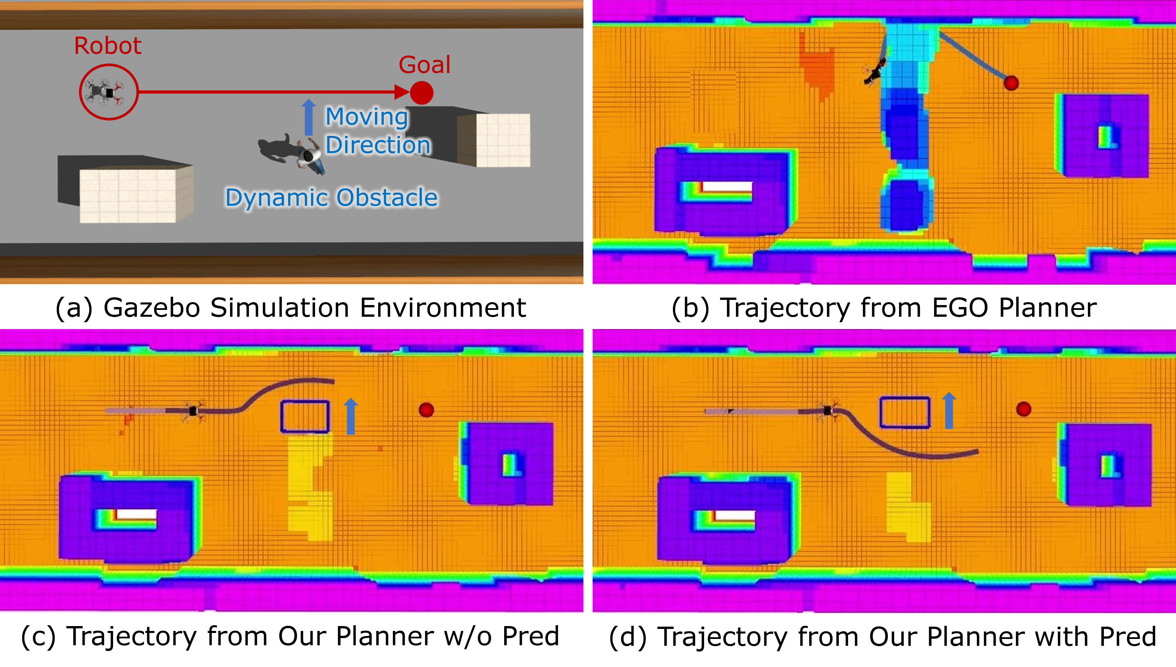
Figure 5: Comparison of generated trajectories from benchmark planners in the same scenario. (a) Experiment scenario in Gazebo. (b) EGO Planner [5] failure due to a noisy map. (c) Our planner's trajectory without prediction, resulting in potential collision. (d) Safe trajectory generated by our planner.

The quantitative results measure the number of collisions for our system and benchmark methods across environments with different difficulty levels, as shown in Fig. 6. The white cylinders are static obstacles, and the red cylinders are dynamic obstacles that move randomly. We selected the EGO planner [5] and ViGO [9] as benchmarks. We also compared the performance of our method with and without the prediction module. Each method was tested 20 times in each environment, and the number of collisions was recorded. The results are shown in Table II. The entries represent the number of collisions, with the values in parentheses indicating the percentage relative to ViGO. Overall, our planner demonstrates the fewest collisions across all three environments. The N/A value for the EGO planner indicates that its trajectory generation fails due to noisy maps in the medium and high-density environments. Comparing the number of collisions for ViGO with our method without prediction reveals that our method achieves a lower collision rate even though ViGO uses linear prediction for dynamic obstacles. From our experimental observations, when a dynamic obstacle is close to the robot, the trajectory generated by B-spline trajectory optimization (ViGO) does not allow the robot to maneuver aggressively enough to avoid immediate collisions. In contrast, our method, which uses model predictive control, allows for more agile avoidance maneuvers. Besides, the comparison between our method with and without the prediction module shows that the proposed prediction method effectively reduces collisions, which matches the observations in the qualitative experiments.

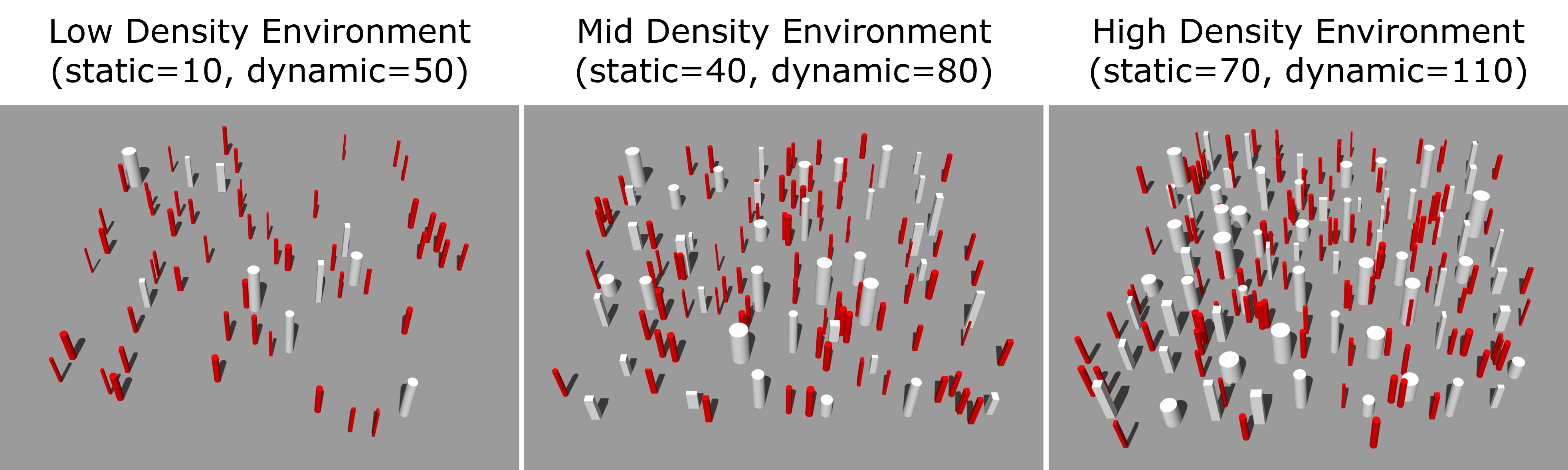
Figure 6: Visualization of experiment environments with varying obstacle densities used to evaluate the number of collisions. Static obstacles are shown in white and dynamic obstacles are displayed in red.

TABLE II: Benchmark of the number of collisions from 20 sample runs in environments with different obstacle densities.

Collision Times Measurement with Benchmarks on a 20m$\times$20m Map
Obstacle Density	Low Density	Mid Density	High Density
	S=10, D=50	S=40, D=80	S=70, D=110
EGO Planner [5]	53 ($196.2\%$)	N/A	N/A
ViGO [9]	27 ($100\%$)	56 ($100\%$)	69 ($100\%$)
Ours w/o pred	12 ($44.4\%$)	25 ($44.6\%$)	43 ($62.3\%$)
Ours	4 (14.8%)	11 (19.6%)	14 (20.3%)

IV-B Physical Flight Tests

To validate the performance of the system in real-world scenarios, we conducted experiments to replicate situations where the robot needs to safely operate alongside humans. We selected two indoor environments and one outdoor environment for conducting the physical flight tests, as illustrated in Fig. 7. In each environment, the robot either builds the map in real-time for straight-line navigation or uses a pre-built map with waypoints to navigate through complex structures. To simulate dynamic obstacles, we let persons intentionally walk toward the robot at a normal walking speed, blocking the robot's paths. The left column images in Fig. 7 capture moments when the robot encounters humans, while the right column images display the generated safe trajectories for collision avoidance. Our observations confirm that the robot successfully navigates safely in all environments, demonstrating the effectiveness of the proposed method.

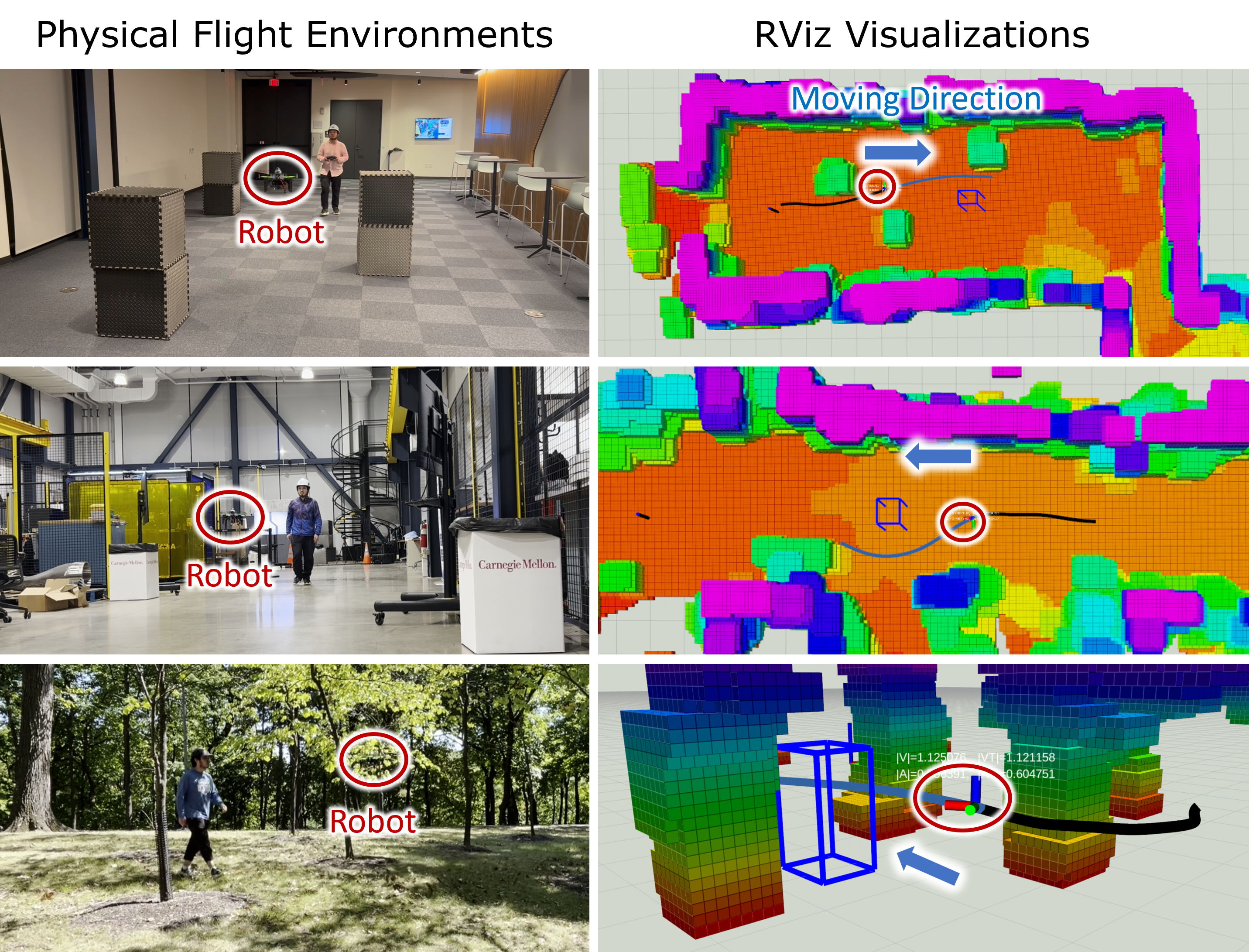
Figure 7: Physical flight experiments. The left column figures show moments of collision avoidance in various environments, while the right column figures visualize the robot following safe trajectories to avoid obstacles.

Since the proposed dynamic perception module is based on a camera with a limited field of view, we also performed experiments using a motion capture system to verify obstacle avoidance ability from all directions, as shown in Fig. 8. In this experiment, the robot hovers at a fixed position while multiple pedestrians walk toward it. As illustrated in Fig. 8, the robot can successfully avoid the pedestrian and return to its original position once the pedestrian moves away.

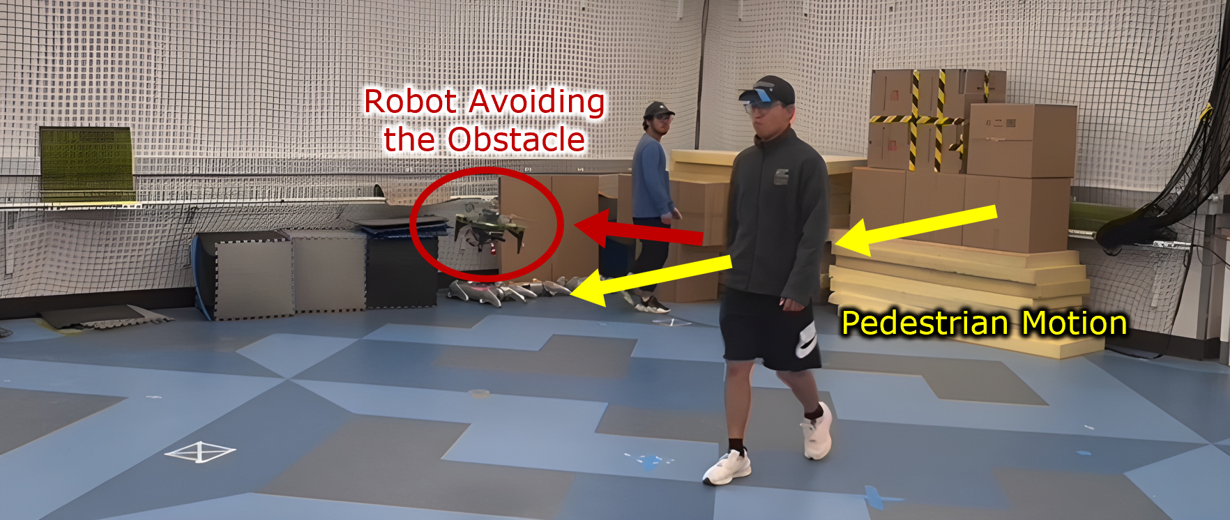
Figure 8: Experiment on collision avoidance Using a motion capture system. The figure illustrates the robot successfully avoiding a dynamic obstacle.

During these experiments, we measured the computation time for each module within the proposed navigation system, as summarized in Table III. It is important to note that all modules run in parallel on separate threads. The perception module, responsible for both static and dynamic perception, requires times of 15 ms and 27 ms, respectively. The dynamic obstacle prediction module, which includes intent and trajectory prediction, demonstrates highly efficient performance, with computation times of 0.05 ms for intent prediction and 2 ms for trajectory prediction. Finally, the planning module shows a computation time of 10 ms for generating a single MPC trajectory, and the total time for intent-based planning, including multiple MPC trajectories, is 68 ms. These results demonstrate that the system components perform within a duration suitable for real-time applications, enabling effective navigation and obstacle avoidance in dynamic environments.

TABLE III: Measurement of Proposed System Computation Time.

Proposed System	Module Component	Comp. Time
Perception Module	Static Perception	$15\text{ms}$
	Dynamic Perception	$27\text{ms}$
Prediction Module	Intent Prediction	$0.05\text{ms}$
	Trajectory Prediction	$2\text{ms}$
Planning Module	MPC Trajectory	$10\text{ms}$
	Intent-based Planning	$68\text{ms}$

V Conclusion and Future Work

This paper introduces a comprehensive autonomous navigation framework to enhance the safety and effectiveness of indoor UAV navigation in dynamic environments. Our approach addresses key challenges in perception and planning by incorporating a dynamic obstacle intent prediction mechanism. Specifically, we develop a perception module that efficiently detects and tracks dynamic obstacles, mitigating issues of tracking loss and occlusion during collision avoidance. We further employ a Markov Decision Process (MDP) in our intent prediction module to anticipate potential actions of dynamic obstacles and generate future trajectories. To ensure safe navigation, we propose an intent-based planning algorithm that leverages model predictive control (MPC) to compute optimal trajectories. Simulation and physical experiments validate the effectiveness of the proposed framework in enabling reliable and safe navigation of aerial robots in complex and dynamic environments. To achieve a better performance in navigating dynamic environments, our future work will focus on integrating a lightweight LiDAR to enhance the tracking range of the current system.

References

- [1] H. Liang, S.-C. Lee, W. Bae, J. Kim, and S. Seo, ``Towards uavs in construction: advancements, challenges, and future directions for monitoring and inspection,'' Drones, vol. 7, no. 3, p. 202, 2023.
- [2] C. Gao, X. Wang, R. Wang, Z. Zhao, Y. Zhai, X. Chen, and B. M. Chen, ``A uav-based explore-then-exploit system for autonomous indoor facility inspection and scene reconstruction,'' Automation in Construction, vol. 148, p. 104753, 2023.
- [3] Z. Xu, B. Chen, X. Zhan, Y. Xiu, C. Suzuki, and K. Shimada, ``A vision-based autonomous uav inspection framework for unknown tunnel construction sites with dynamic obstacles,'' IEEE Robotics and Automation Letters, vol. 8, no. 8, pp. 4983–4990, 2023.
- [4] B. Zhou, F. Gao, L. Wang, C. Liu, and S. Shen, ``Robust and efficient quadrotor trajectory generation for fast autonomous flight,'' IEEE Robotics and Automation Letters, vol. 4, no. 4, pp. 3529–3536, 2019.
- [5] X. Zhou, Z. Wang, H. Ye, C. Xu, and F. Gao, ``Ego-planner: An esdf-free gradient-based local planner for quadrotors,'' IEEE Robotics and Automation Letters, vol. 6, no. 2, pp. 478–485, 2020.
- [6] Z. Xu, X. Zhan, Y. Xiu, C. Suzuki, and K. Shimada, ``Onboard dynamic-object detection and tracking for autonomous robot navigation with rgb-d camera,'' IEEE Robotics and Automation Letters, vol. 9, no. 1, pp. 651–658, 2024.
- [7] J. Lin, H. Zhu, and J. Alonso-Mora, ``Robust vision-based obstacle avoidance for micro aerial vehicles in dynamic environments,'' in 2020 IEEE International Conference on Robotics and Automation (ICRA), 2020, pp. 2682–2688.
- [8] Y. Wang, J. Ji, Q. Wang, C. Xu, and F. Gao, ``Autonomous flights in dynamic environments with onboard vision,'' in 2021 IEEE/RSJ International Conference on Intelligent Robots and Systems (IROS), 2021, pp. 1966–1973.
- [9] Z. Xu, Y. Xiu, X. Zhan, B. Chen, and K. Shimada, ``Vision-aided uav navigation and dynamic obstacle avoidance using gradient-based b-spline trajectory optimization,'' in 2023 IEEE International Conference on Robotics and Automation (ICRA), 2023, pp. 1214–1220.
- [10] H. Chen, C.-Y. Wen, F. Gao, and P. Lu, ``Flying in dynamic scenes with multitarget velocimetry and perception-enhanced planning,'' IEEE/ASME Transactions on Mechatronics, 2023.
- [11] D. Mellinger and V. Kumar, ``Minimum snap trajectory generation and control for quadrotors,'' in 2011 IEEE international conference on robotics and automation. IEEE, 2011, pp. 2520–2525.
- [12] C. Richter, A. Bry, and N. Roy, ``Polynomial trajectory planning for aggressive quadrotor flight in dense indoor environments,'' in Robotics Research: The 16th International Symposium ISRR. Springer, 2016, pp. 649–666.
- [13] O. Khatib, ``Real-time obstacle avoidance for manipulators and mobile robots,'' The international journal of robotics research, vol. 5, no. 1, pp. 90–98, 1986.
- [14] J. Van Den Berg, S. J. Guy, M. Lin, and D. Manocha, ``Reciprocal n-body collision avoidance,'' in Robotics Research: The 14th International Symposium ISRR. Springer, 2011, pp. 3–19.
- [15] Y. Ren, S. Liang, F. Zhu, G. Lu, and F. Zhang, ``Online whole-body motion planning for quadrotor using multi-resolution search,'' in 2023 IEEE International Conference on Robotics and Automation (ICRA). IEEE, 2023, pp. 1594–1600.
- [16] H. Oleynikova, D. Honegger, and M. Pollefeys, ``Reactive avoidance using embedded stereo vision for mav flight,'' in 2015 IEEE International Conference on Robotics and Automation (ICRA). IEEE, 2015, pp. 50–56.
- [17] B. Guo, N. Guo, and Z. Cen, ``Obstacle avoidance with dynamic avoidance risk region for mobile robots in dynamic environments,'' IEEE Robotics and Automation Letters, vol. 7, no. 3, pp. 5850–5857, 2022.
- [18] W. Liu, Y. Ren, and F. Zhang, ``Integrated planning and control for quadrotor navigation in presence of suddenly appearing objects and disturbances,'' IEEE Robotics and Automation Letters, 2023.
- [19] M. Pantic, I. Meijer, R. Bähnemann, N. Alatur, O. Andersson, C. Cadena, R. Siegwart, and L. Ott, ``Obstacle avoidance using raycasting and riemannian motion policies at khz rates for mavs,'' in 2023 IEEE International Conference on Robotics and Automation (ICRA). IEEE, 2023, pp. 1666–1672.
- [20] H. Zhu and J. Alonso-Mora, ``Chance-constrained collision avoidance for mavs in dynamic environments,'' IEEE Robotics and Automation Letters, vol. 4, no. 2, pp. 776–783, 2019.
- [21] T. Wakabayashi, Y. Suzuki, and S. Suzuki, ``Dynamic obstacle avoidance for multi-rotor uav using chance-constraints based on obstacle velocity,'' Robotics and Autonomous Systems, vol. 160, p. 104320, 2023.
- [22] Z. Jian, Z. Yan, X. Lei, Z. Lu, B. Lan, X. Wang, and B. Liang, ``Dynamic control barrier function-based model predictive control to safety-critical obstacle-avoidance of mobile robot,'' in 2023 IEEE International Conference on Robotics and Automation (ICRA). IEEE, 2023, pp. 3679–3685.
- [23] G. Chen, P. Peng, P. Zhang, and W. Dong, ``Risk-aware trajectory sampling for quadrotor obstacle avoidance in dynamic environments,'' IEEE Transactions on Industrial Electronics, vol. 70, no. 12, pp. 12 606–12 615, 2023.
- [24] T. Eppenberger, G. Cesari, M. Dymczyk, R. Siegwart, and R. Dubé, ``Leveraging stereo-camera data for real-time dynamic obstacle detection and tracking,'' in 2020 IEEE/RSJ International Conference on Intelligent Robots and Systems (IROS). IEEE, 2020, pp. 10 528–10 535.
- [25] A. J. Sathyamoorthy, U. Patel, T. Guan, and D. Manocha, ``Frozone: Freezing-free, pedestrian-friendly navigation in human crowds,'' IEEE Robotics and Automation Letters, vol. 5, no. 3, pp. 4352–4359, 2020.
- [26] V. Tolani, S. Bansal, A. Faust, and C. Tomlin, ``Visual navigation among humans with optimal control as a supervisor,'' IEEE Robotics and Automation Letters, vol. 6, no. 2, pp. 2288–2295, 2021.
- [27] R. Peddi, C. Di Franco, S. Gao, and N. Bezzo, ``A data-driven framework for proactive intention-aware motion planning of a robot in a human environment,'' in 2020 IEEE/RSJ International Conference on Intelligent Robots and Systems (IROS). IEEE, 2020, pp. 5738–5744.
- [28] H. Thomas, J. Zhang, and T. D. Barfoot, ``The foreseeable future: Self-supervised learning to predict dynamic scenes for indoor navigation,'' IEEE Transactions on Robotics, 2023.
- [29] A. Alahi, K. Goel, V. Ramanathan, A. Robicquet, L. Fei-Fei, and S. Savarese, ``Social lstm: Human trajectory prediction in crowded spaces,'' in Proceedings of the IEEE conference on computer vision and pattern recognition, 2016, pp. 961–971.
- [30] A. Gupta, J. Johnson, L. Fei-Fei, S. Savarese, and A. Alahi, ``Social gan: Socially acceptable trajectories with generative adversarial networks,'' in Proceedings of the IEEE conference on computer vision and pattern recognition, 2018, pp. 2255–2264.
- [31] H. Cui, V. Radosavljevic, F.-C. Chou, T.-H. Lin, T. Nguyen, T.-K. Huang, J. Schneider, and N. Djuric, ``Multimodal trajectory predictions for autonomous driving using deep convolutional networks,'' in 2019 international conference on robotics and automation (icra). IEEE, 2019, pp. 2090–2096.
- [32] K. D. Katyal, G. D. Hager, and C.-M. Huang, ``Intent-aware pedestrian prediction for adaptive crowd navigation,'' in 2020 IEEE International Conference on Robotics and Automation (ICRA). IEEE, 2020, pp. 3277–3283.
- [33] T. Benciolini, D. Wollherr, and M. Leibold, ``Non-conservative trajectory planning for automated vehicles by estimating intentions of dynamic obstacles,'' IEEE Transactions on Intelligent Vehicles, vol. 8, no. 3, pp. 2463–2481, 2023.
- [34] J. Zhou, B. Olofsson, and E. Frisk, ``Interaction-aware motion planning for autonomous vehicles with multi-modal obstacle uncertainty predictions,'' IEEE Transactions on Intelligent Vehicles, 2023.
- [35] S. Shi, C. Guo, L. Jiang, Z. Wang, J. Shi, X. Wang, and H. Li, ``Pv-rcnn: Point-voxel feature set abstraction for 3d object detection,'' in Proceedings of the IEEE/CVF conference on computer vision and pattern recognition, 2020, pp. 10 529–10 538.
- [36] W. Xu, Y. Cai, D. He, J. Lin, and F. Zhang, ``Fast-lio2: Fast direct lidar-inertial odometry,'' IEEE Transactions on Robotics, vol. 38, no. 4, pp. 2053–2073, 2022.