ModCube: Modular, Self-Assembling Cubic Underwater Robot

Abstract

This paper presents a low-cost, centralized modular underwater robot platform, ModCube, which can be used to study swarm coordination for a wide range of tasks in underwater environments. A ModCube structure consists of multiple ModCube robots. Each robot can move in six DoF with eight thrusters and can be rigidly connected to other ModCube robots with an electromagnet controlled by onboard computer. In this paper, we present a novel method for characterizing and visualizing dynamic behavior, along with four benchmarks to evaluate the morphological performance of the robot. Analysis shows that our ModCube design is desirable for omnidirectional tasks, compared with the configurations widely used by commercial underwater robots. We run real robot experiments in two water tanks to demonstrate the robust control and self-assemble of the proposed system, We also open-source the design and code to facilitate future research: https://jiaxi-zheng.github.io/ModCube.github.io/.

I Introduction

Underwater robots have allowed us to explore the vast benthic world, even reaching the deepest regions of the ocean, the Mariana Trench [1]. However, these robots are often costly to build and limited to their designed tasks: The shape of an underwater robot is typically specific to its designated application and does not generalize to other tasks. This lack of flexibility presents barriers to more widespread research and commercial deployments of underwater robots. To tackle this, we present a low-cost MSRR platform [2], which we call ModCube. Individual ModCube robots are agile and omnidirectional, while a swarm of ModCubes can dock with each other to reconfigure into different shapes for diverse tasks.

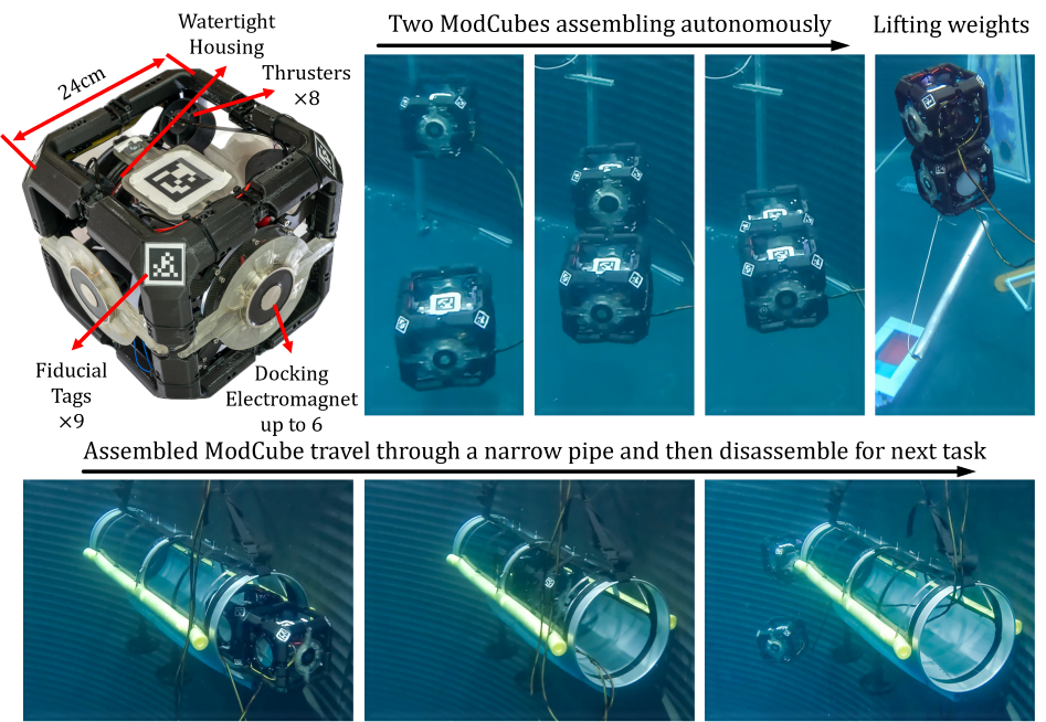
Figure 1: ModCube’s design (top left) features 8 thrusters allowing omnidirectional motion and docking mechanism for assemble and reconfiguration. Two ModCubes can assemble into a holistic structure autonomously. With this assembled structure we show the capability of lifting a metal pipe from the bottom of the tank, passing through a narrow pipe, and disassemble for reconfiguration.

The underwater environment presents unique opportunities for the development of MSRR. The assembled structure can be configured in a more diverse way as the robot moves in six DoF (DoF). In comparison, most of the terrestrial or airborne swarm robots are physically constrained, resulting in limited connection patterns. For example, groups of UGV generally cannot connect to each other from below. Likewise, quadrotors have limited vertical connection areas due to gravity and aerodynamic constraints. These constraints are not applicable underwater, which ModCube leverages to its advantage. Underwater robots also face unique challenges in modeling the dynamics. Particular attention has been paid to durability and energy efficiency. However, it can often be challenging to accurately estimate some of the robot’s physical properties to accurately model the robot’s dynamical behavior in the water.

With these opportunities and challenges in mind, we present a comprehensive analysis of ModCube and dive into the details of its design. We focus on producing a modular underwater robot designed for self-assembly and enhanced agility. In particular, the design of ModCube, especially the configuration of its actuation components, was carefully analyzed to ensure mobility and stability. This led to a design consisting of a symmetric frame structure equipped with eight thrusters to achieve omnidirectional movement and high agility. We also endow ModCube with an innovative docking mechanism designed to take advantage of the reduced connectivity constraints underwater, providing a connection bridge for ModCube. In light of the challenges of analyzing underwater robots, we propose a novel method using morphological characteristic analysis, which we apply to quantify and characterize the mobility of ModCube. This analysis provides a clear visualization of the robot’s dynamics based on spherical harmonics [3]. Our analysis highlights ModCube’s superior mobility and power efficiency.

In summary, this paper presents an underwater MSRR, ModCube, along with extensive analysis of its design. Concretely, we provide the following technical contributions:

1. The design details of the ModCube system.

2. A novel morphological characterization method for robot dynamics analysis, which can be applied to a range of underwater robots.

3. Real-world experiments in a water tank which rigorously validates the proposed platform, mechanism and software.

II Related Work

II-A Shape design of underwater vehicles

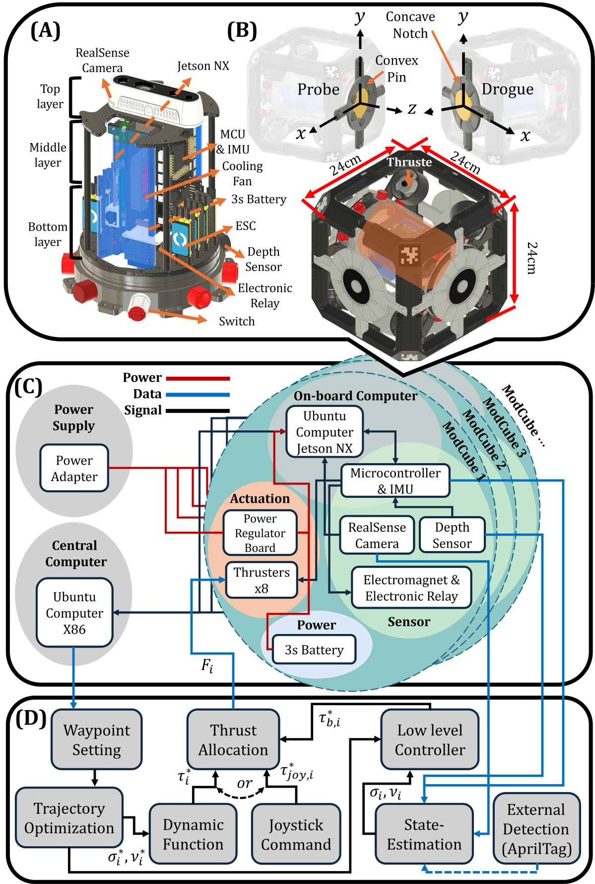
Figure 2: System components and architecture. (A) Interior view of ModCube. (B) Exterior view of ModCube with the cabin highlighted in orange, and the docking mechanism layout in the top. (C) Electronic system architecture. (D) Control and planning framework.

The design of underwater robots varies a lot based on the task requirements. Full-size ROV are frequently used for underwater manipulation tasks, but their large size often results in limited mobility [4]. In contrast, compact-size ROV are typically box-shaped and equipped with five to eight thrusters, allowing omnidirectional maneuverability for tasks such as underwater inspection [5]. However, the hydrodynamic performance of ROV is poor and mobility is often limited. For long-range autonomous tasks, torpedo-shaped [6] or dual-hulled AUV [7] have been widely used, which have streamlined shapes for travelling longer distances. In summary, all today’s underwater robots are designed for a single purpose that does not generalize to different tasks [8]. In this paper, we aim to develop a modular robot system that can be potentially versatile for various tasks through self-assembly.

II-B Underwater robot for compact space

Compared with conventional underwater robots designed for open water, the small-scale underwater robot is perfectly built for compact space inspection, such as nuclear fuel facilities on sites where the human is restricted from entering [9], operations in shallow water areas [10], and even interacts with underwater animals [11]. Although mobility is highlighted, existing compact-sized underwater robots do not support onboard computation well. Therefore, they all have limited extendability towards online deep learning, 3D mapping, or state estimation stacks. Researchers have deployed Jetson computers on tiny quadrotors and performed autonomous swarm operations in the field [12].

II-C Reconfigurable robot swarms

Research in MSRR focuses on deploying multiple robots to dynamically form task-specific structures tailored to diverse operational needs [13]. Significant progress has been made in air and ground environments. For example, the ground-based car SMORES-EP [14] can explore unknown environments by reactively reconfiguring itself. Similarly, bio-inspired robots, like the multilegged robot [15], can perform diverse tasks in variable terrains. In the aerial domain, the Modquad [16] demonstrates a stable integration of multiple units.

However, research specific to underwater environments remains limited. Early work, such as CoCoRo (CoCoRo) [17], exhibited restricted mobility due to its fish-like actuated form. Other studies have explored implicit coordination resembles fish swarms [18], but do not show possibilities for assembling or reconfiguring. Other approaches require human intervention to preconfigure robots before actions [19].

III ModCube Design

ModCube is designed to travel, assemble, and reconfigure in the 3D underwater environment with six DoF. A single ModCube features a cubic shape that is symmetric in shape, mass distribution, and thruster configuration. Each ModCube is equipped with four electromagnets, which allows them to dock with each other and move as a rigid body.

III-A System Overview

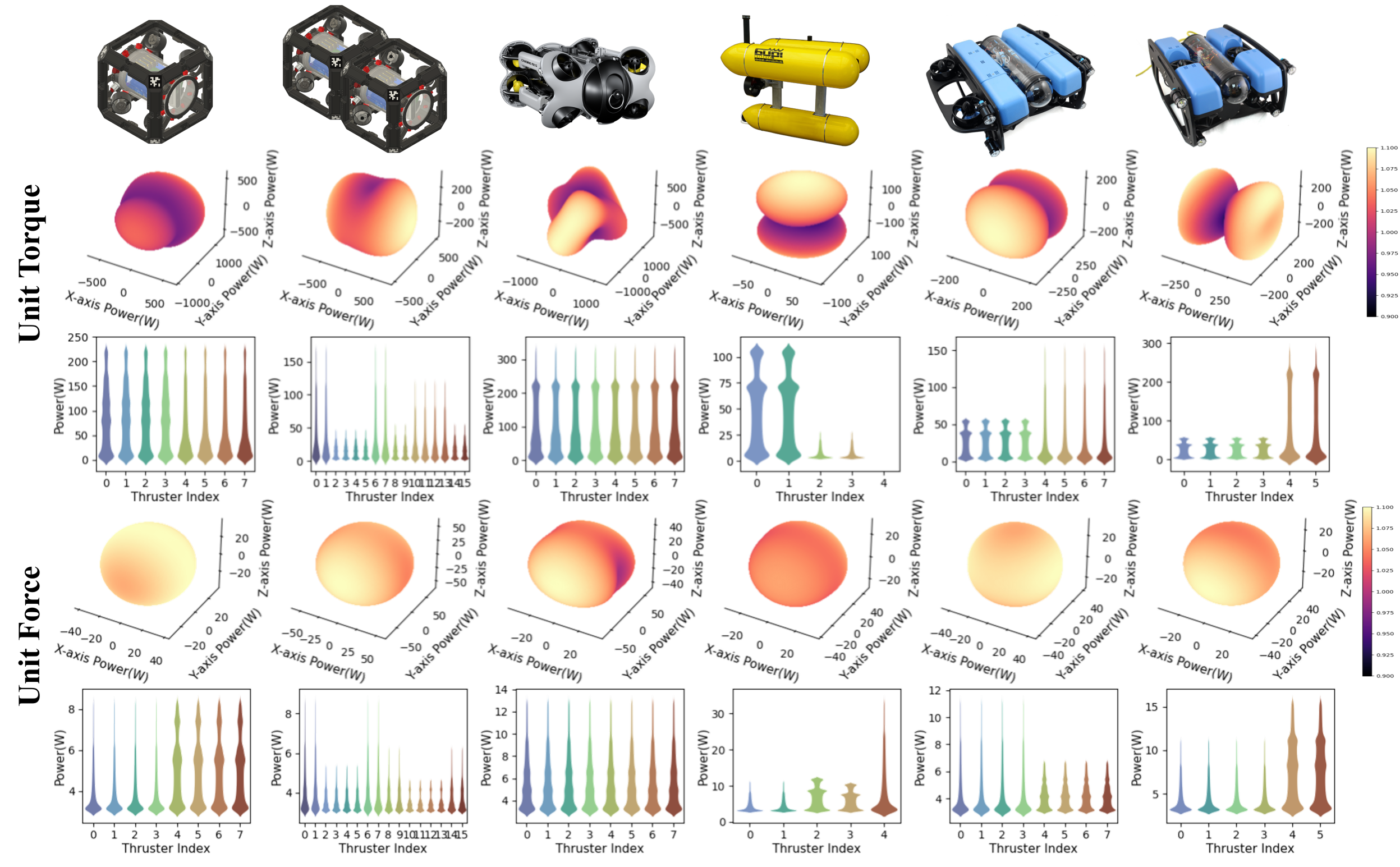
Figure 3: Benchmark comparisons of six popular commercial underwater robots: The 3D heatmap visualizes the power consumption as a vector field under a given unit torque and force. The violin plot illustrates the distribution of power consumption across individual thrusters. The numerical results of the morphological analysis in Table I follow the same order as the robots listed.

The following features are highlighted for each ModCube (also see Fig. 2(A)):

Onboard Computer: ModCube integrates an Nvidia Jetson NX computer, providing a platform for high level perception, planning, and control tasks.

Minimization: We organize electronic components into 3 layers to optimize internal space for electronics following a bottom-up design strategy (* denote optional components):

• Bottom layer: Electric relay, Battery*, ESC (ESC)

• Middle layer: microcontroller, Linux computer*, Power distribution board

• Top layer: USB camera*

Dual power supply: Our design allows users to power ModCube with external power supply or on-board batteries.

Low Cost: ModCube features a jet-fusion nylon PA12 material for the cowling of the 56mm customized diameter thruster with a waterproof brushless motor, and 3D-printed aluminum for the propeller. Each thruster provides a maximum thrust of 10N, withstands pressures up to 50m deep, and costs only 14 USD each.

Fabrication: ModCube’s mechanical structure features a dual-layer outer shell, featuring a metal frame for structural support and a nylon shell for collision protection. The shell’s mounting holes facilitate the attachment of various components such as docking disks, manipulators, DVL, and sonar, supporting our modular use case.

III-B Docking Mechanism Design

A robust docking mechanism that allows robots to dock and detach smoothly is essential for self-assembly. Previous work on robot docking inspired us by using electromagnets and docking disks [20, 21]. In our design, an electronic relay controls the power on/off of the electromagnet. Additionally, We designed a guidance rail for the docking disk that provides an initial positioning tolerance of 4 mm and a rotational tolerance of 50 degrees, also preventing any relative rotation between the two disks during docking. ModCube’s disks consist of two types: Probe and Drogue, as shown in Fig. 2 (B). The docking disks feature a circular arrangement of alternately positioned convex pins and concave notches, viewed from the side projection, ensures that the Probe and Drogue disks interlock securely. The docking disk is made from the same material as the shell, with circular constraint slots on the outer surface to maintain rotational alignment between two ModCubes.

Successful docking is identified by monitoring the pulse of current on the electromagnet. Docking is successful if the current value drops above 650mA. Validation with real-robot experiments are discussed in V-B and Fig. 7 (A).

III-C Morphological Characterization

TABLE I: Comprehensive Analysis of Thrust Allocation Parameters for Various Underwater Robots

		Single ModCube	Double ModCube	Chasing	Girona 500 AUV	BlueROV2 Heavy	BlueROV2
Price (USD)$\downarrow$		800	1600	2500	7000+	4500	6000
Size (mm³)		210x210x210	430x210x210	380x267x165	1500x1000x1000	457x338x254	457x436x254
Given unit Torque	Dirichlet Energy $E_{D}\downarrow$	$1.577e+07$	$6.898e+06$	$4.613e+07$	$1.211e+06$	$3.195e+06$	$9.673e+06$
	Willmore Energy $\mathcal{W\downarrow}$	$2.475e+22$	$6.496e+15$	$1.019e+17$	$4.523e+20$	$8.323e+11$	$2.248e+23$
	Power Cost (W)$\downarrow$	$5.613e+07$	$4.065e+07$	$7.596e+07$	$1.050e+07$	$2.256e+07$	$2.550e+07$
	Variance Volume$\downarrow$	$3.393e+07$	$7.774e+06$	$5.059e+07$	$7.479e+06$	$7.930e+06$	$2.851e+07$
Given unit Force	Dirichlet Energy $E_{D}\downarrow$	$2.234e+03$	$1.422e+04$	$4.848e+04$	$8.509e+03$	$3.911e+03$	$3.193e+03$
	Willmore Energy $\mathcal{W\downarrow}$	$3.045e+14$	$3.754e+15$	$7.430e+22$	$1.131e+16$	$1.600e+15$	$6.885e+15$
	Power Cost (W)$\downarrow$	$3.314e+06$	$5.606e+06$	$4.209e+06$	$2.900e+06$	$3.255e+06$	$3.062e+06$
	Variance Volume$\downarrow$	$2.071e+04$	$7.371e+03$	$4.827e+04$	$1.763e+05$	$2.250e+04$	$7.633e+04$

One of the design goals of ModCube is omnidirectional mobility that allows agile reconfiguration. The design of ModCube structure and thruster allocation take into consideration the force and torque can be generated in arbitrary direction. Concretely, to generate a unit force or unit torque in an arbitrary direction, we look at how the power consumption is distributed over all directions (Fig. 3).

Such distribution can be visualized as a closed 3D surface [22], initially composed of a fixed number of vertices forming a sphere, which is then scaled according to specific parameters such as power consumption or hydrodynamic effects. The smoothness of this surface directly reflects the continuity and stability of its operations [23]. For ModCube, ensuring smooth steering and locomotion is crucial for maintaining precise control and effective task execution in complex environments. The variance of thruster effort is also important to ensure hardware lifespan. The volume of the 3D closed surface also reflects the total power consumption.

We employ two metrics from geometric analysis: Willmore energy $\mathcal{W}$ [24] and Dirichlet energy $E_{D}$ [25], to analyze the smoothness of a three-dimensional surface. Willmore energy can be calculated by [24]:

$$\mathcal{W}=\sum_{i}^{n}H_{i}^{2}A_{i}-\sum_{i}^{n}K_{i}A_{i}$$ (1)

$H_{i}$ is the mean curvature at vertex $i$, $K_{i}$ is the Gaussian curvature at vertex $i$, $A_{i}$ is the area associated with vertex $i$ calculated by Delaunay tool, The summation is performed over all vertices.

Dirichlet energy can be calculated by [25]:

$$E_{D}=\sum_{l=0}^{l_{\text{max}}}\sum_{m=-l}^{l}l(l+1)\left|\sum_{i}^{n}d_{i}Y_{l}^{m}\right|^{2}$$ (2)

where $d_{i}$ is the radial distance for each vertex $i$. $Y_{l}^{m}$ is the spherical harmonic function at vertex $i$. The outer sum over $l_{\text{max}}=10$ and $m$ sums over all spherical harmonic modes, with the factor $l(l+1)$ representing the contribution of the harmonic degree to the energy. The summation over $i$ inside the absolute value accounts for the least-squares fit of the radial distances using spherical harmonics.

The result is presented in Table I and Fig. 3, showcasing four popular commercial underwater robots, each equipped with different thruster numbers $n_{t}$ ranging from five to eight and various allocations. In Fig. 3, the 3D heatmap illustrates the magnitude of the total power consumption, while the violin graph represents the distribution of the power consumption. A more uniform power distribution indicates smoother control transitions for ModCube.

Among the robots listed in Table I, single ModCube has the lowest price and the minimum size. In comparison, Chasing M2 exhibits the most balanced distribution, offering near-uniform directionality, but at the cost of higher power consumption. Girona 500 exhibits the lowest energy consumption, suggesting the smoothest performance under a given unit torque, but suffers from uneven thrust distribution. ModCube excels across these metrics, particularly in force application, which is crucial in underwater robotics due to the expansive, unobstructed environment where less emphasis is placed on turning.

IV Model and Control

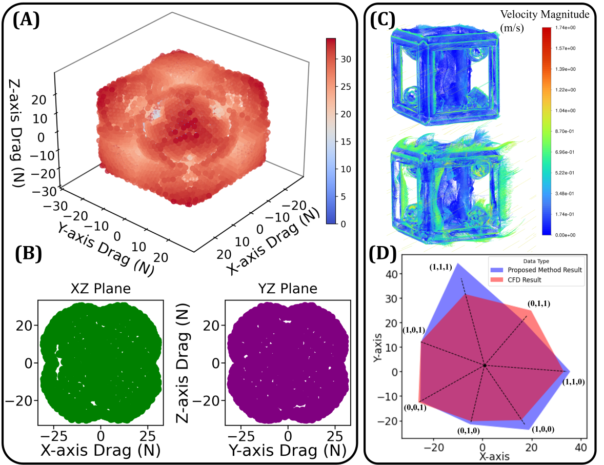
Figure 4: (A) Vector-valued hydrodynamics field by proposed method. (B) XZ and YZ plane (C) Flow velocity pathline in Ansys Fluent simulation with a ModCube. (D) Comparison of the drag force calculated by the proposed method and simulation result.

IV-A Robot Hydrodynamics

Underwater robots overcomes significant darg force while moving in water. For efficient trajectory planning and following, it is critical to characterize the darg force. The drag force on a single ModCube is formulated using the NASA (NASA) drag equation:

$$\boldsymbol{\tau}_{D}=\frac{1}{2}C_{d}\rho av_{f}^{2}$$ (3)

where the drag coefficient $C_{d}$ is computed using CFD (CFD) simulations in Ansys Fluent with a flow velocity of $v_{f}=1\,\text{m/s}$, $\rho$ is the fluid density, and $a$ is the frontal area. The frontal area orthogonal to the velocity, is calculated using the Monte Carlo method. the detailed process is discussed later in Algorithm 1. Satisfies $\boldsymbol{\tau}_{D}/||\boldsymbol{\tau}_{D}||=v_{f}/||v_{f}||$.

The visualization details of ModCube show a near symmetrical surface area and omnidirectional hydrodynamic properties indicated by proposed method in Fig. 4 (A) (B) and CFD simulations in Fig. 4 (C). It can be treated as having an identical shape due to minimal variance in results. We compare the calculated results from Algorithm 1 with the reference results obtained from CFD, as shown in Fig. 4 (D). The figure displays drag forces across seven flow directions. The significant deviations caused by the vertices create a sharper leading edge, which streamlines the flow and reduces the formation of turbulent wake regions behind the object. This streamlined flow results in lower energy loss and, consequently, reduced overall drag forces on the object.

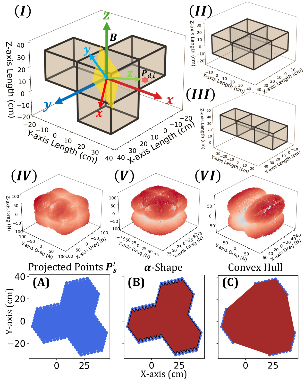
Figure 5: Construction of a ModCube structure following Algorithm 1. The top row (I to III) illustrates different ModCube structures: random, box, and line configurations. The middle row (IV to VI) depicts the corresponding relative drag force vector fields. The body frame $\mathcal{B}$ is shown in I, with the projection plane highlighted in yellow. The random index $P_{d,i}$ is indicated by a red star, and the shallow green arrow represents the drag vector. The bottom row (A) displays $P_{s}^{\prime}$ in blue, with the estimated shapes shown in red, using the $\alpha$-convex shape and convex hull tool, respectively.

Algorithm 1 Hydrodynamics of Arbitrary Configuration

1:Input: $P_{s},n_{s},v_{f},\rho,C_{d}$

2:Output: $\Psi$

3:for $i=0$ to $n_{s}-1$ do

4:    $\varphi_{i}=\arccos\left(1-\frac{2i}{n_{s}}\right),\theta_{i}=\pi\left(1+\sqrt{5}\right)i$

5:    $P_{d}\leftarrow(\cos(\theta_{i})\sin(\varphi_{i}),\sin(\theta_{i})\sin(\varphi_{i}),\cos(\varphi_{i}))$

6:end for

7:for  ${p}_{i}\in P_{d},\{i\in n_{s}\}$ do

8:    $\mathbf{e}_{z}=[0,0,1]^{\top}$, ${v}_{i}={p}_{i}\times\mathbf{e}_{z}$, $c_{i}={p}_{i}\mathbf{e}_{z}$, $s_{i}=\|{v}_{i}\|$

9:    ${R}_{i}=\mathbf{I}_{3\times 3}+{K(v)}_{i}+{K(v)}_{i}^{2}\left(\frac{1-c_{i}}{s_{i}^{2}}\right),{K}^{\top}=-{K}$

10:    $P_{s}^{\prime}=({R}_{i}P_{s})\mathbf{e}_{z}$

11:    $C_{l}=\texttt{$\alpha$-shape}(P_{s}^{\prime})$

12:    $\Psi_{i}=\frac{1}{2}C_{d}\rho C_{l}v_{f}^{2}{p}_{i}$ using Eq. 3

13:end for

14:return $\Psi$

IV-B Monte Carlo Approximation of Hydrodynamics

When an assembled ModCube structure moves, the direction of motion can make a significant difference in the hydrodynamics depending on the robot configuration. We also approximate the drag force with the frontal area for an assembled ModCube structure. To determine the frontal area of an arbitrary configuration, we sample points inside ModCube uniformly and use orthographic projection to project the sample points $P_{s}$ from the body frame $\mathcal{B}\rightarrow\mathbb{R}^{3}$ into the projection plane orthogonal to the velocity direction (yellow color as shown in Fig. 5$(I)$).

In Algorithm 1 we use $\alpha$-shape to estimate the best shape representing the compressed sample points $P_{s}^{\prime}$ [26] as the frontal area, the result shown as Figure 5(B), and (C) demonstrates the estimated result of convex hull tool [27], which failed to capture the concavities and holes present in a random structure shape.

IV-C Thrust Allocation

For a single ModCube, give a control input $u$, a thruster consumes power $P$ and generates a force $f$. Their relationship is modeled using polynomial functions:

$$f(u)=c_{u}\boldsymbol{\beta}(u), P(f)=c_{f}\boldsymbol{\beta}(f)$$ (4)

Here, $\boldsymbol{\beta}(x)=[1,x,x^{2},\ldots,x^{5}]^{T}$ represents the vector of polynomial basis functions, while $c_{u}$ and $c_{f}$ denote the polynomial parameter matrices. The overall force and moment exerted on the vehicle are calculated as follows:

$${T}=\sum_{i=1}^{n_{t}}\left[\begin{matrix}p_{i}^{t}\\ r_{i}^{t}\times p_{i}^{t}\end{matrix}\right],\quad F={T}^{+}\boldsymbol{\tau}$$ (5)

where $\boldsymbol{\tau}\in\mathbb{R}^{6\times 1}$ is the given wrench(force/torque) vector, ${\quad F}\in\mathbb{R}^{n_{t}\times 1}$ is the thrust maticx($n_{t}$ is the number of the thruster), and ${T}$ is the kinematic transformation matrix, ${T}^{+}$ is the pseudo-inverse of ${T}$. The position vector $r_{i}^{t}$ and rotation vector $p_{i}^{t}$ extend from the vehicle’s center of mass to each thruster. The sum of the power is then computed by:

$$\mathcal{P}=\sum_{i=1}^{n_{t}}P(f)$$ (6)

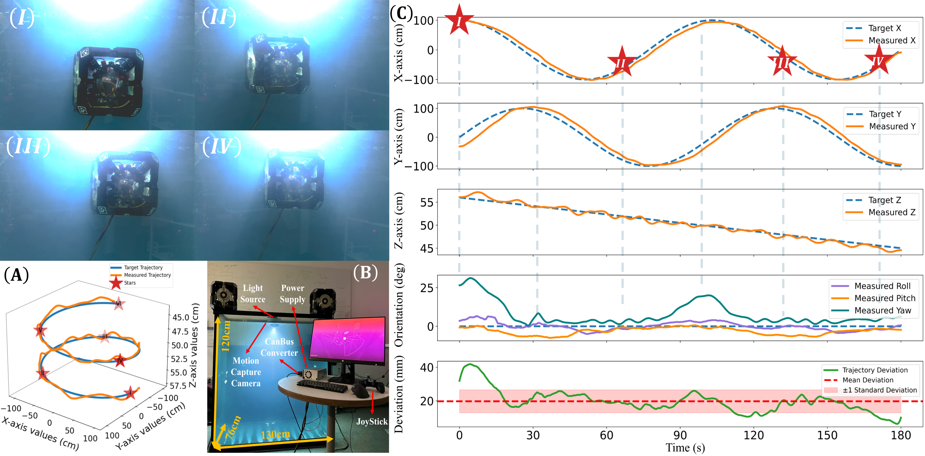
Figure 6: Cylindrical spiral trajectory tracking from supplementary video clips S1. I-IV shows snapshots of the tracking process. (A) ModCube target trajectory and measured trajectory in 3D space. (B) The lab water tank experiment layout. (C) Position and attitude while tracking the target trajectory: The measured trajectory is shown as a solid line, and the target trajectory is shown as a dash line, highlighting key events marked by red stars. The bottom right graph shows trajectory deviation over time. The green line shows the trajectory deviation, the red dashed line represents the mean deviation, and the pink shaded area indicates the ±1 standard deviation.

IV-D ModCube Dynamics

Following Fossen’s formulation [28], the general dynamics of underwater robots are expressed in matrix-vector notation. The position and attitude of a single ModCube are parameterized by the body-fixed velocities $\boldsymbol{\nu}\in\mathbb{R}^{6}$, while the world-fixed velocities are represented by $\boldsymbol{\eta}\in\mathbb{R}^{6}$. The kinematic relationship is:

$$\dot{\boldsymbol{\eta}}=J(\boldsymbol{\eta})\boldsymbol{\nu}$$ (7)

The single ModCube’s dynamic model is given by:

$$M\dot{\boldsymbol{\nu}}+C(\boldsymbol{\nu})\boldsymbol{\nu}+D_{A}(\boldsymbol{\nu})\boldsymbol{\nu}+g(\boldsymbol{\eta})=\boldsymbol{\tau}+\boldsymbol{\tau}_{D}$$ (8)

where $M$ is the combined mass matrix including rigid body and added mass effects, $C(\boldsymbol{\nu})$ accounts for Coriolis and centrifugal forces, $D_{A}(\boldsymbol{\nu})$ represents hydrodynamic damping, $g({\eta})$ includes buoyancy and gravitational forces. The forces and moments generated by the actuators are represented by $\tau$. External forces and moments on the robot are neglected, and $\boldsymbol{\tau}_{D}$ represents drag forces. Additionally, the center of gravity and the center of buoyancy are designed to coincide, resulting in $g(\eta)=0$.

For a ModCube structure, the system functions as a rigid body with 6 degrees of freedom. The geometric center is set as ModCube structure’s center, and the dynamic model for ModCube is described by $\hat{M}=J^{\top}\text{diag}(M_{1},\ldots,M_{\mathcal{N}})J$, and similar definitions apply for $\hat{C}$ and $\hat{D}_{A}$, $\mathcal{N}$ refers to the number of ModCubes within the structure.

IV-E ModCube Control

The ModCube system can be operated in two control modes: 1) autonomous mode, where the system automatically follows a predefined trajectory; 2) teleoperated mode, allowing an operator to control the ModCube using a joystick. Throughout the experiment, each ModCube maintains a hovering state, regulated by a feedback control loop (see Fig 2(D)), ensuring that the attitude angles $(\phi_{i},\theta_{i},\psi_{i}$), $i\in\mathcal{N}$ remain at zero. The position is given by $(x_{i},y_{i},z_{i})$, and the state vector is $\boldsymbol{\sigma_{i}}=[x_{i},y_{i},z_{i},\phi_{i},\theta_{i},\psi_{i}]$ , $\boldsymbol{\nu_{i}}=\dot{\boldsymbol{\sigma_{i}}}$.

The objective is to guide each ModCube to follow a predefined trajectory. The high-level trajectory planner computes the control inputs $\boldsymbol{\tau}$ based on ModCube’s current global position and the target location using a cascade PID controller defined as below:

$${\nu_{i}}^{*}=K_{p}^{1}({\sigma_{i}}^{*}-{\sigma_{i}})+K_{i}^{1}\int({\sigma_{i}}^{*}-{\sigma_{i}})\,dt+K_{d}^{1}({\sigma_{i}}^{*}-{\sigma_{i}})$$

$${\tau}_{i}^{*}=K_{p}^{2}({\nu}_{i}^{*}-{\nu}_{i})+K_{i}^{2}\int({\nu}_{i}^{*}-{\nu}_{i})\,dt+K_{d}^{2}({\nu}_{i}^{*}-{\nu}_{i})$$ (9)

Here, $K_{p}$, $K_{i}$, and $K_{d}$ represent the proportional, integral, and derivative gains, and the numbers in the upper right denote the controller layer. respectively. The superscripts denote the layer number of the PID controller. The superscripts with * mean the desired values.

V Experiments

Two experiments were conducted to evaluate ModCube’s capabilities. The first experiment, cylindrical spiral trajectory tracking, assessed ModCube’s fundamental control performance, which is a prerequisite for complex swarm tasks. Building on this, the second experiment focused on advanced docking to establish the feasibility of more intricate self-assembly tasks.

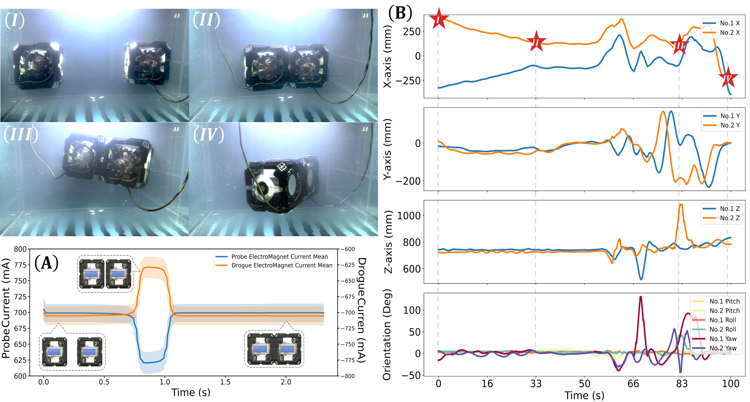
Figure 7: Snapshots of the hovering self-assembly and structure steering experiment from supplementary video clips S2 - S3. I-IV Sequential images of the automatic docking process: I Initial positions, II Successful docking. III-IV Sequential images of structure locomotion with teleoperation. The Electromagnet current values were measured during docking in over ten experiments shown in (A). The (B) on the right illustrates the X, Y, and Z-axis displacements and attitude (pitch, roll, yaw) over time, highlighting key events marked by red stars.

The experiments are conducted within a $130\times 120\times 76\,\text{cm}$ water tank, see Fig. 6 (B). The tank is equipped with a camera to track the robot motion. For all experiments, we attached a large (10cm$\times$10cm) Apriltag [29] to the top of each ModCube. Each vertex of the robot was also equipped with smaller (3cm$\times$3cm) Apriltags to increase the tracking robustness in real-time, at 60hz. In addition, a submerged LED provides a light source for the environment. The CANbus converter serves as the hub for ModCube’s CAN signal. The power supply outputs 12V DC, while a joystick controller, with an emergency button, is used for mode transfer.

V-A Cylindrical Spiral Trajectory Tracking

We evaluate the performance of our control approach by executing a cylindrical spiral trajectory tracking task over a 180-second period. The ModCube initiates the task at the bottom of the tank and ascends along the defined spiral path shown as Fig. 6 I–VI, controlled by a PID algorithm. The tracking results, illustrated in Fig. 6, demonstrate the system’s capability to follow the target trajectory with minimal error. The instabilities, likely caused by hydrodynamic forces and thruster interactions, diminish as the system converges to the desired trajectory, showing improved stability over time.

The deviation plot in Fig. 6 (C) quantifies the Euclidean distance between the actual and target positions, illustrating the system’s tracking accuracy. Initially, the deviation spikes to 40 mm within the first 20 seconds, likely due to controller initialization and system calibration. Afterward, the deviation stabilizes around 20 mm, as indicated by the mean deviation line. The pink-shaded region, representing ±1 standard deviation, shows that the system maintains consistent tracking accuracy within this range throughout the experiment.

The attitude control data (pitch, roll, yaw) further highlight the system’s ability to maintain stable orientation during the task. Minor fluctuations are observed during ascent but are successfully corrected, demonstrating the ModCube’s robustness in compensating for external disturbances and maintaining precise trajectory alignment.

V-B Self-assembly

Following successful trajectory tracking, we conducted an experiment with two ModCubes assemble into a rigid structure, as shown in Fig. 7. The ModCubes, starting from opposite sides of the tank, follow a straight-line trajectory and dock with each other using electromagnets, as illustrated in snapshots (I) to (VI), forming a two-member ModCube structure. The assembled structure was then teleoperated to assess its locomotion.

Figure 7 (A) shows electromagnet current measurements during docking. The shaded regions indicate the variability across ten trials, while the solid lines represent the mean current for the probe and drogue electromagnets. A sharp pulse at approximately 1.0s marks successful engagement, followed by current stabilization, confirming a secure connection. Figure 7 (B) presents time-series data for X, Y, and Z-axis displacements during docking. Oscillations in the X-axis, highlighted by red stars, reflect positional instabilities due to proximity effects induced by the thrusters. After docking, the displacement data converge reflecting a successful alignment. Attitude plots (pitch, roll, yaw) show instability during approach, but stabilize post-docking. This highlights the system’s ability to self-correct after assembly.

We observed slight instabilities in position and attitude prior to assembly, likely caused by the interaction of jet flows from the close proximity of the thrusters. Additionally, the limited tank space and proximity to the wall of the water tank cause these instabilities.

V-C Demonstrations of Use Cases

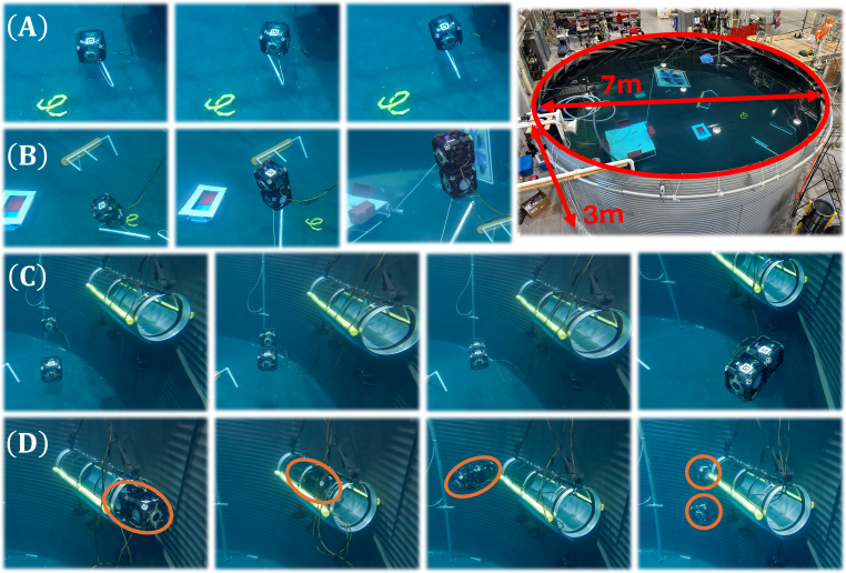
Figure 8: Snapshots from (A) to (D) sequentially illustrate: (A) unsuccessful attempt of a single ModCube lifting a metal pipe, (B) successful weight-lifting task with two ModCubes, (C) docking procedure of two separate ModCubes, and (D) in-pipe traversal and disassembly task following docking. Above tasks deployed in the CMU Highbay water tank are referenced in supplementary video clips S4 - S8.

Fig. 8 illustrates the capabilities of the ModCube system in various underwater tasks, including use cases for cooperative object lifting, autonomous docking, and in-pipe traversing. These scenarios demonstrate the modularity, adaptability, and precise control of the system in complex environments. The ability to reconfigure and execute coordinated maneuvers highlights the potential of ModCube for advanced underwater operations.

VI Conclusion and Future Work

This paper introduced ModCube, a novel modular underwater robot designed for self-assembly and reconfiguration. Our approach leverages morphological analysis to construct a vector field, and effectively quantifies the robot’s dynamics through the surface smoothness of the field. We validate the attach and detach functionality between ModCubes with a horizontal docking configuration. Based on the success of our developed docking mechanism, we demonstrate the capability of assembled ModCube like weight lifting and narrow space locomotion. To address this, future work will involve the assembly of more ModCube units and exploring its capabilities in self-assembly-based collective manipulation. We also plan to use graph optimization methods to optimize the thrust configuration to find the best configuration, based on our proposed morphological characterization. This will extend ModCube’s operational capabilities and enhance energy efficiency in more complex underwater environments.

References

- [1] Andrew D. Bowen et al. “The Nereus hybrid underwater robotic vehicle for global ocean science operations to 11,000m depth” In OCEANS 2008, 2008, pp. 1–10 DOI: 10.1109/OCEANS.2008.5151993
- [2] Mark Yim et al. “Modular self-reconfigurable robot systems [grand challenges of robotics]” In IEEE Robotics & Automation Magazine 14.1 IEEE, 2007, pp. 43–52
- [3] Sheldon Axler, Paul Bourdon and Ramey Wade “Harmonic function theory” Springer Science & Business Media, 2013
- [4] Amy Phung et al. “Enhancing scientific exploration of the deep sea through shared autonomy in remote manipulation” In Science Robotics 8.81, 2023, pp. eadi5227 DOI: 10.1126/scirobotics.adi5227
- [5] Edward Morgan, William Ard and Corina Barbalata “A Probabilistic Framework For Hydrodynamic Parameter Estimation for Underwater Manipulators” In OCEANS 2023 - MTS/IEEE U.S. Gulf Coast, 2023, pp. 1–9 DOI: 10.23919/OCEANS52994.2023.10337120
- [6] Geoffrey A. Hollinger et al. “Learning Uncertainty in Ocean Current Predictions for Safe and Reliable Navigation of Underwater Vehicles” In Journal of Field Robotics 33.1, 2016, pp. 47–66 DOI: https://doi.org/10.1002/rob.21613
- [7] Hanumant Singh et al. “Seabed AUV offers new platform for high-resolution imaging” In Eos, Transactions American Geophysical Union 85.31 Wiley Online Library, 2004, pp. 289–296
- [8] Junku Yuh and Michael West “Underwater robotics” In Advanced Robotics 15.5 Taylor & Francis, 2001, pp. 609–639
- [9] Arron Griffiths et al. “AVEXIS—Aqua vehicle explorer for in-situ sensing” In IEEE Robotics and Automation Letters 1.1 IEEE, 2016, pp. 282–287
- [10] Killian Poore, Christopher Kitts, Geoffrey Wheat and William Kirkwood “A small scale ROV for shallow-water science operations” In OCEANS 2016 MTS/IEEE Monterey, 2016, pp. 1–6 IEEE
- [11] Robert K Katzschmann, Joseph DelPreto, Robert MacCurdy and Daniela Rus “Exploration of underwater life with an acoustically controlled soft robotic fish” In Science Robotics 3.16 American Association for the Advancement of Science, 2018, pp. eaar3449
- [12] Xin Zhou et al. “Swarm of micro flying robots in the wild” In Science Robotics 7.66 American Association for the Advancement of Science, 2022, pp. eabm5954
- [13] Kirstin H Petersen et al. “A review of collective robotic construction” In Science Robotics 4.28 American Association for the Advancement of Science, 2019, pp. eaau8479
- [14] Jonathan Daudelin et al. “An integrated system for perception-driven autonomy with modular robots” In Science Robotics 3.23 American Association for the Advancement of Science, 2018, pp. eaat4983
- [15] Yasemin Ozkan-Aydin and Daniel I Goldman “Self-reconfigurable multilegged robot swarms collectively accomplish challenging terradynamic tasks” In Science Robotics 6.56 American Association for the Advancement of Science, 2021, pp. eabf1628
- [16] David Saldana et al. “Modquad: The flying modular structure that self-assembles in midair” In 2018 IEEE International Conference on Robotics and Automation (ICRA), 2018, pp. 691–698 IEEE
- [17] James Paulos et al. “Automated self-assembly of large maritime structures by a team of robotic boats” In IEEE Transactions on Automation Science and Engineering 12.3 IEEE, 2015, pp. 958–968
- [18] Florian Berlinger, Melvin Gauci and Radhika Nagpal “Implicit coordination for 3D underwater collective behaviors in a fish-inspired robot swarm” In Science Robotics 6.50 American Association for the Advancement of Science, 2021, pp. eabd8668
- [19] Jing Zhou, Sideng Hu, Tiefeng Li and Xiangning He “Cubic marine robotics” In Nature Reviews Electrical Engineering 1.3 Nature Publishing Group UK London, 2024, pp. 143–144
- [20] Stefano Mintchev, Raffaele Ranzani, Filippo Fabiani and Cesare Stefanini “Towards docking for small scale underwater robots” In Autonomous Robots 38 Springer, 2015, pp. 283–299
- [21] Francesco Branz, Lorenzo Olivieri, Francesco Sansone and Alessandro Francesconi “Miniature docking mechanism for CubeSats” In Acta Astronautica 176 Elsevier, 2020, pp. 510–519
- [22] Mike Allenspach et al. “Design and optimal control of a tiltrotor micro-aerial vehicle for efficient omnidirectional flight” In The International Journal of Robotics Research 39.10-11 SAGE Publications Sage UK: London, England, 2020, pp. 1305–1325
- [23] Gerald Farin “Curves and surfaces for CAGD: a practical guide” Elsevier, 2001
- [24] Alexander I. Bobenko and Peter Schröder “Discrete Willmore Flow” In ACM SIGGRAPH 2005 Courses, SIGGRAPH ’05 Association for Computing Machinery, 2005, pp. 5–es DOI: 10.1145/1198555.1198664
- [25] Richard Courant “Dirichlet’s principle, conformal mapping, and minimal surfaces” Courier Corporation, 2005
- [26] Herbert Edelsbrunner, David Kirkpatrick and Raimund Seidel “On the shape of a set of points in the plane” In IEEE Transactions on information theory 29.4 IEEE, 1983, pp. 551–559
- [27] C Bradford Barber, David P Dobkin and Hannu Huhdanpaa “The quickhull algorithm for convex hulls” In ACM Transactions on Mathematical Software (TOMS) 22.4 Acm New York, NY, USA, 1996, pp. 469–483
- [28] Thor I Fossen “Handbook of marine craft hydrodynamics and motion control” John Wiley & Sons, 2011
- [29] John Wang and Edwin Olson “AprilTag 2: Efficient and robust fiducial detection” In 2016 IEEE/RSJ International Conference on Intelligent Robots and Systems (IROS), 2016, pp. 4193–4198 IEEE