Logarithmic Subdiffusion from a Damped Bath Model

Abstract

A damped heat bath is a modification of the standard oscillator heat bath model, wherein each bath oscillator itself has a Markovian coupling to its own heat bath. We modify such a model as described in Plyukhin (2019) to one where the oscillators undergo linear rather than constant damping, and find that this generates a memory kernel which behaves like $k(t)\sim 1/t$ as $t\to\infty$ when the spectral density is Ohmic. This is a boundary case not considered in previous works. As the memory kernel does not have a finite integral, it is subdiffusive, and we numerically show the diffusion to go as $\left\langle{\Delta Q^{2}(t)}\right\rangle\sim t/\log(t)$ as $t\to\infty$. We also numerically calculate the velocity correlation function in the asymptotic regime and use it to confirm the aforementioned subdiffusion.

I Introduction

Brownian motion gives rise to so-called normal diffusion, where the mean-squared displacement $\left\langle{\Delta Q^{2}}\right\rangle=\left\langle{(Q-\left\langle{Q}\right\rangle)^{2}}\right\rangle$ of the position $Q$ of a free particle is asymptotically linear in time. This motion is found in nature: for example the random movement of a large particle such as pollen suspended in a liquid or gaseous medium, as first modelled by Einstein Einstein (1905).

Some systems will exhibit superdiffusion, where the mean-squared displacement increases faster than linearly in the asymptotic time regime. A simple example is a ballistic particle; more interesting examples include atmospheric eddies such as smoke and turbulence Richardson (1926). Conversely, some systems exhibit subdiffusion, where the mean-squared displacement is sub-linear. This can be due to crowding effects such as those occurring in biological systems Weiss et al. (2004); Regner et al. (2013). These examples of anomalous diffusion are typically described in terms of a power law mean-square displacement $\left\langle{\Delta Q^{2}(t)}\right\rangle\sim t^{\alpha}$, where $\alpha>1$ corresponds to superdiffusion and $\alpha<1$ indicates subdiffusion.

Diffusion is studied in both classical and quantum systems and in both cases, normal diffusion is effectively modelled using the Langevin equation driven by a thermal stochastic force. Anomalous diffusion is typically modelled by modifying the Langevin equation to achieve non-standard properties, such as modifying the statistics of the stochastic force Jespersen et al. (1999). Alternatively, one can replace the dissipation term with a convolution integral of the velocity and a memory kernel — the so-called generalised Langevin equation — which can describe information back-flow into the system. One can then study the diffusive effects of different memory kernels Porrà et al. (1996). In particular, if the memory kernel behaves asymptotically as $k(t)\sim t^{-\alpha}$ where $0<\alpha<1$, then the system will be subdiffusive, with $\left\langle{\Delta Q^{2}(t)}\right\rangle\sim t^{\alpha}$ Plyukhin (2019); Kupferman (2004).

Classically, one can modify the equivalent Fokker-Planck equation by replacing ordinary derivatives with fractional derivatives Metzler et al. (1999); Metzler and Klafter (2000). This can also be done with the Langevin equation itself Grigolini et al. (1999); Lutz (2001a). In the quantum case one can introduce fractional derivatives in the master equation to study anomalous quantum diffusion Tarasov (2013). Quantum mechanical systems are more subtle due to low temperature quantum effects which often change the diffusion properties; indeed a high-temperature limit is often taken for simplicity.

Both classically and quantum mechanically, the generalised Langevin equation can be derived from a simple open systems model where a system of interest interacts with a bath composed of harmonic oscillators Ford et al. (1965); Cortés et al. (1985); Caldeira and Leggett (1983). Anomalous diffusion can then be modelled by appropriately changing the interaction between system and bath, that is the distribution of oscillator frequencies and the coupling between each oscillator and the system. In particular, a choice of a spectral density linear in frequency with an infinite frequency cut-off leads to delta correlated noise and Markovian evolution. More generally, different power-law spectral densities correspond to more exotic diffusive behaviour, and the corresponding mean-squared displacement does not necessarily follow a power-law Grabert et al. (1987). Alternatively one can consider fractional coupling between the bath and system Vertessen et al. (2024) or random interaction Hamiltonians Lutz (2001a, b). In quantum mechanical systems, a zero-temperature heat bath can lead to subdiffusion Breuer and Petruccione (2002).

An alternative approach is proposed in Plyukhin (2019), whereby the internal structure of the bath is changed: using instead a damped bath model to generate a memory kernel with the aforementioned power law. This model consists of a system coupled to a bath of harmonic oscillators, with each oscillator in turn coupled to its own bath of harmonic oscillators (see fig. 1). The interaction between each primary bath oscillator and it’s corresponding bath is presumed to be Markovian. One can consider this damped bath model as a particle interacting with a bath of Brownian particles instead of harmonic oscillators.

In this paper we show that a simple modification to this model can be used to generate a subdiffusive boundary case. We modify the model to allow the damping of each primary oscillator bath to be proportional to the frequency. With this modification the memory behaves asymptotically as $k(t)\sim 1/t$ even with a linear (Ohmic) spectral density; a non-linear power-law spectral density is not required. It is the internal structure of the bath which causes it to respond to the system according to an infinite time-scale, leading to anomalous diffusion.

This power-law behaviour is a boundary case of the range considered above, and is not readily represented as a fractional derivative. However since it is non-integrable, it still results in subdiffusion Morgado et al. (2002), although the diffusion not governed by a power-law. We show numerically that the mean-squared displacement asymptotically behaves like $\left\langle{\Delta Q^{2}(t)}\right\rangle\sim t/\log(t)$, and confirm this diffusion using the velocity autocorrelation function. This diffusive behaviour does not arise from the standard Caldeira-Leggett model with a power-law spectral density, at any temperature Grabert et al. (1987).

II Damped Bath Model

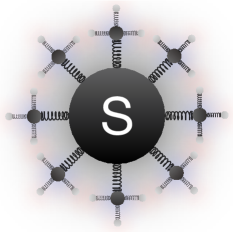
Figure 1: Schematic of damped bath model. The system of interest is coupled to a collection of harmonic oscillators, each of which is in turn coupled to their own set of harmonic oscillators. The secondary baths induce Markovian dissipation in each oscillator of the primary bath. This modified bath structure will lead to subdiffusion without changing the nature of coupling (i.e. the spectral density) between the system of interest and the primary bath.

The model consists of a single position degree of freedom $Q$, and associated momentum $P$, coupled linearly to a bath of $N$ harmonic oscillators $\left\{q_{k},p_{k}\right\}_{k=1}^{N}$. The Hamiltonian consists of three terms

$$H=H_{\textsc{s}}+H_{\textsc{b}}+H_{\textsc{int}}.$$ (1)

The system and interaction parts are given by

$$H_{\textsc{s}} =\frac{P^{2}}{2M}+\sum_{n=1}^{N}\frac{g_{n}^{2}}{2m_{n}\omega_{n}^{2}}Q^{2}$$ (2a)

$$H_{\textsc{int}} =-\sum_{n=1}^{N}g_{n}q_{n}Q,$$ (2b)

where the quadratic system term counters the potential re-normalisation induced from the interaction of the system and the bath. The bath Hamiltonian term $H_{\textsc{b}}$ has the usual kinetic and quadratic potential terms but to each oscillator we add an extra Hamiltonian term $H_{\textsc{b}}^{(n)}$

$$H_{\textsc{b}}=\sum_{n=1}^{N}\left(\frac{p_{n}^{2}}{2m_{n}}+\frac{m_{n}\omega_{n}^{2}q_{n}^{2}}{2}+H_{\textsc{b}}^{(n)}\right),$$ (3)

where $H_{\textsc{b}}^{(n)}$ is an entire secondary harmonic bath Hamiltonian consisting of $N_{n}$ oscillators coupled linearly to the $n^{\text{th}}$ oscillator,

$$H_{\textsc{b}}^{(n)}=\sum_{\nu=1}^{N_{n}}\left(\frac{p_{n,\nu}^{2}}{2m_{n,\nu}}+\frac{m_{n,\nu}\omega_{n,\nu}^{2}}{2}\left(q_{n,\nu}-\frac{g_{n,\nu}}{m_{n,\nu}\omega_{n,\nu}^{2}}q_{n}\right)^{2}\right).$$ (4)

Here $q_{n,\nu}$ and $p_{n,\nu}$ are the position and momentum respectively of the $\nu^{\text{th}}$ oscillator in the secondary bath corresponding to the $n^{\text{th}}$ oscillator of the primary bath. Instead of a standard harmonic equation of motion, the equation of motion of the $n^{\text{th}}$ primary bath oscillator takes the form of a generalised Langevin equation, owing to the interaction with the secondary bath,

$$\ddot{q}_{n}+\omega_{n}^{2}q_{n}+\int_{0}^{t}k_{n}(t-t^{\prime}) \dot{q}_{n}(t^{\prime})\,dt^{\prime}+k_{n}(t)q_{n}(0)$$

$$=\frac{1}{m_{n}}\varepsilon_{n}(t)+\frac{g_{n}}{m_{n}}Q.$$ (5)

The memory kernel $k_{n}$ and the stochastic force $\varepsilon_{n}$ are given by the familiar expressions for the standard oscillator environmental model Breuer and Petruccione (2002). The stochasticity of $\varepsilon_{n}(t)$ arises from the (thermal) uncertainty of the initial conditions $q_{n,\nu}(0)$ and $p_{n,\nu}(0)$. Assuming a standard Ohmic spectral density for each secondary bath, the primary bath equation of motion becomes that of a damped and driven harmonic oscillator,

$$\ddot{q}_{n}+2\gamma_{n}\dot{q_{n}}+\omega_{n}^{2}q_{n}=\frac{g_{n}}{m_{n}}Q+\frac{1}{m_{n}}\varepsilon_{n}(t),$$ (6)

where $\gamma_{n}$ is the damping coefficient of the $n^{\text{th}}$ oscillator, and the factor of $2$ is included for convenience. Since the probability distribution for the initial conditions is thermal at temperature $T$, the stochastic forces $\varepsilon_{n}(t)$ have the usual white noise statistics,

$$\left\langle{\varepsilon_{n}(t)}\right\rangle=0,\;\;\left\langle{\varepsilon_{n}(t)\varepsilon_{j}(t^{\prime})}\right\rangle=4k_{B}Tm_{n}\gamma_{n}\delta(t-t^{\prime})\delta_{ij}$$ (7)

where $k_{B}$ is Boltzmann’s constant. The homogeneous solution to (6) is

$$q_{n}^{(h)}(t)=a_{n}(t)q_{n}(0)+b_{n}(t)p_{n}(0),$$ (8)

where

$$a_{n}(t) =e^{-\gamma_{n}t}\left(\cos\Omega_{n}t+\frac{\gamma_{n}}{\Omega_{n}}\sin\Omega_{n}t\right),$$ (9a)

$$b_{n}(t) =\frac{1}{m_{n}\Omega_{n}}e^{-\gamma_{n}t}\sin\Omega_{n}t,$$ (9b)

and $$\Omega_{n}^{2}=\omega_{n}^{2}-\gamma^{2}_{n} \sum_{n}g_{n}b_{n}(t)$$. The green’s function for the particular solution is ; and so the equation of motion for the system of interest is itself a generalised Langevin equation,

$$M\frac{d^{2}Q}{dt}+\int_{0}^{t} k(t-t^{\prime})\dot{Q}(t^{\prime})\,dt^{\prime}+k(t)Q(0)=f(t)$$ (10)

with a memory kernel and stochastic force which show the effect of the secondary bath coupling,

$$k(t) =\sum_{n=1}^{N}\frac{g_{n}^{2}}{m_{n}\omega_{n}^{2}}a_{n}(t),$$ (11a)

$$f(t) =\sum_{n=1}^{N}\left(g_{n}q_{n}^{(h)}(t)+g_{n}\int_{0}^{t}b_{n}(t-t^{\prime})\varepsilon_{n}(t^{\prime})\,dt^{\prime}\right).$$ (11b)

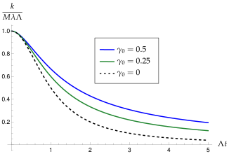
Figure 2: Memory kernel for the damped bath model with an Ohmic spectral density with an exponential cut-off. The kernel is plotted for $\gamma_{0}=0,0.25,0.5$. When $\gamma_{0}=0$, then $k(t)\sim 1/t^{2}$, and the kernel has a finite integral over the positive real line, giving a finite bath time-scale. When $\gamma_{0}>0$, then $k(t)\sim 1/t$, which has an infinite time scale, leading to subdiffusion.

Assuming the initial condition of the primary bath is a thermal state at temperature $T$ (the same temperature as the secondary baths) in the quantum case, or has thermally distributed initial conditions, the fluctuation-dissipation relation holds,

$$\frac{1}{2}\left\langle{\left\{f(t),f(t^{\prime})\right\}}\right\rangle=k_{B}Tk(|t-t^{\prime}|),$$ (12)

where $\left\{\cdot,\cdot\right\}$ denotes the anti-commutator. In the quantum case the high-temperature limit must be taken so that the ground state fluctuations become negligible.

We re-write the memory kernel in the integral form,

$$k(t)=\int_{0}^{\Lambda}\frac{J(\omega)}{\omega}a_{\omega}(t)\,d\omega$$ (13)

where $\Lambda$ is the maximal oscillator frequency and $a_{\omega}(t)$ is simply $a_{n}(t)$ with $\gamma_{n}\to\gamma(\omega)$, and $\Omega_{n}\to\Omega(\omega)$; and $J(\omega)$ is the spectral density

$$J(\omega)=\sum_{n=1}^{N}\frac{g_{n}^{2}}{m_{n}\omega_{n}^{2}}\delta(\omega-\omega_{n}).$$ (14)

In contrast to Plyukhin (2019) we now assume a linear damping of oscillators $\gamma(\omega)=\gamma_{0}\omega$. We assume that $0<\gamma_{0}<1$ for convenience but this is not a necessary restriction. The frequency shift then becomes $\Omega(\omega)=\omega\sqrt{1-\gamma_{0}^{2}}=\gamma_{1}\omega$. The type of diffusion arising from this memory kernel can be determined from the integral of the memory kernel over the positive real axis Morgado et al. (2002),

$$\int_{0}^{\infty}k(t)\,dt=\int_{0}^{\Lambda}\frac{2\gamma_{0}J(\omega)}{\omega^{2}}\,d\omega.$$ (15)

The diffusion will be subdiffusive when this integral is infinte, which happens when the spectral density is asymptotically linear or sub-linear as $\omega\to 0$. Normal diffusion occurs when the integral is finite but non-zero. This happens when the spectral density is asymptotically super-linear. Note that since $J(\omega)>0$, there is no choice of spectral density which could make this integral zero (even using a minimal frequency cut-off as suggested in Morgado et al. (2002)). That is, there is no way to generate superdiffusion using a damped bath model. For comparison, if we followed the choice in Plyukhin (2019) that $\gamma(\omega)=\gamma$ is a constant, then

$$\int_{0}^{\infty}k(t)\,dt=\int_{0}^{\Lambda}\frac{2\gamma J(\omega)}{\omega^{3}}\,d\omega,$$ (16)

and subdiffusion will result from any spectral density that is quadratic or sub-quadratic in $\omega$.

We now make the standard assumption of a continuum of oscillators with an Ohmic spectral density where the maximal frequency is implemented using an exponential cut-off,

$$J(\omega)=M\lambda\omega e^{-\frac{\omega}{\Lambda}},$$ (17)

with $\lambda$ as a dissipation constant. As mentioned above, any power-law spectral density with a larger exponent in $\omega$ will no longer lead to a non-integrable kernel, necessary for subdiffusion. The memory kernel can now be calculated

$$k(t) =M\lambda\int_{0}^{\infty}e^{-\frac{\omega}{\Lambda}}a_{\omega}(t)\,d\omega$$

$$=\frac{M\lambda\Lambda(1+2\gamma_{0}\Lambda t)}{1+2\gamma_{0}\Lambda t+\Lambda^{2}t^{2}}$$ (18)

Asymptotically, this memory kernel behaves as $k(t)\sim 1/t$ as $t\to\infty$. If we choose $\gamma_{0}=0$ (that is turn off the interaction between the primary and secondary baths), then the kernel reverts to $k(t)\sim 1/t^{2}$, which has a finite integral on $[0,\infty)$. It is therefore the presence of the secondary bath which causes the time-scale in which the bath responds to the system of interest to be infinite (see fig. 2).

III Subdiffusion

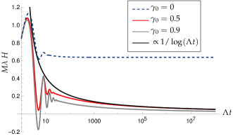
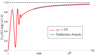
Figure 3: (a) The Green’s function $H$ (20) for the memory kernel (18), computed numerically for values $\gamma_{0}=0,0.5,0.9$, along with the asymptotic fit of $1/\log(t)$ (black) which should apply to the $\gamma_{0}=0.5$ case. When $\gamma_{0}=0$, the secondary bath is turned off and the Green’s function approaches a constant value, as in standard theory. In the asymptotic regime the fit is very accurate. (b) The Green’s function normalised by the inverse logarithm function (red) showing convergence to unity. In blue is plotted the inverse Laplace transform of (22), showing agreement in the asymptotic limit.

The generalised Langevin equation (10) can be solved using Laplace transforms Porrà et al. (1996); Ford and O’Connell (2001), and from this, the mean-squared displacement $\left\langle{Q^{2}(t)}\right\rangle$ is given by

$$\left\langle{\Delta Q^{2}(t)}\right\rangle =\int_{0}^{t}\int_{0}^{t}H(t-t_{1})H(t-t_{2})$$

$$\qquad\qquad\times\left\langle{\left\{f(t_{1}),f(t_{2})\right\}}\right\rangle\,dt_{1}dt_{2}$$ (19)

$$=2k_{B}T\int_{0}^{t}\int_{0}^{t}H(t_{1})H(t_{2})k(|t_{1}-t_{2}|)\,dt_{1}dt_{2}.$$

Here the Green’s function $H(t)$ is defined through its Laplace transform,

$$\int_{0}^{\infty}H(t)e^{-st}\,dt=\frac{1}{Ms^{2}+s\tilde{k}(s)},$$ (20)

where $\tilde{k}(s)$ is the Laplace transform of the memory kernel. In the case of (18), we have the expression

$$\tilde{k}(s)=-\frac{M\lambda}{\pi\gamma_{1}} e^{\frac{s}{\Lambda}(\gamma_{0}-i\gamma_{1})}(\gamma_{0}-i\gamma_{1})^{2}$$ (21)

$$\times\left(\pi+i\,\text{Ei}\left(-\frac{s}{\Lambda}(\gamma_{0}-i\gamma_{1})\right)\right)+\textsc{h.c.},$$

where Ei denotes the exponential integral. Results from Tauberian theory Feller (1991) connect the asymptotic behaviour of a function to the behaviour of its Laplace derivative around zero. In this spirit we see that $\tilde{k}(s)$ behaves as $\tilde{k}(s)\sim-2M\lambda\gamma_{0}\log(s)$ as $s\to 0$. Consequently,

$$\frac{1}{Ms^{2}+s\tilde{k}(s)}\sim-\frac{1}{2M\lambda\gamma_{0}s\log(s)}\quad\text{as}\;s\to 0.$$ (22)

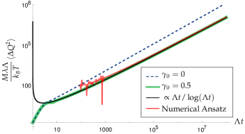
Figure 4: Log-log plot of the mean-squared displacement $\left\langle{\Delta Q^{2}}\right\rangle$ calculated numerically using (19) where $H$ was computed numerically as in fig. 3 with a choice of $\gamma_{0}=0.5$ (green) and $\gamma_{0}=0$ (blue, dashed). When $\gamma_{0}=0$, the system undergoes standard linear diffusion. When $\gamma_{0}>0$ the system undergoes subdiffusion, asymptotically as $\left\langle{\Delta Q^{2}}\right\rangle\sim t/\log(t)$. This behaviour is fitted in black. In red is the result of choosing $H$ to be precisely the asymptotic expression (23); which has a highly oscillatory initial phase but which gives the same asymptotic subdiffusion.

The Green’s function $H(t)$ (20) cannot be calculated analytically but can be evaluated numerically. In fig. 3 we have plotted $H(t)$ corresponding to the memory kernel $k(t)$ (18) in the asymptotic limit. We can see by plotting a fitting curve that asymptotically it behaves as $H(t)\sim 1/\log(t)$ as $t\to 0$. The same asymptotic behaviour is seen when numerically calculating the inverse Laplace transform of (22). The form of (22) suggests that the the parameter dependence is

$$H(t)\sim\frac{1}{2M\lambda\gamma_{0}\log(\Lambda t)},$$ (23)

and this is confirmed numerically. When $\gamma_{0}=0$, the memory kernel becomes integrable, and $H(t)$ asymptotes to a constant value $2/M\lambda\pi$.

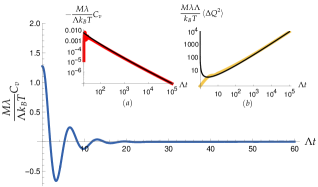
Figure 5: Velocity correlation function $C_{v}$ on linear scales as a function of the dimensionless time parameter $\Lambda t$. Numerically calculated using (27), with $\dot{H}$ derived from $H$, numerically computed in fig. 3. Here $\gamma_{0}=0.5$, and $\Lambda t_{0}$ was chosen to be large enough such that $C_{v}$ became independent of $\Lambda t_{0}$ (in these plots it was set to $\Lambda t_{0}=10^{5}$. Insets: (a) log-log plot of $-C_{v}$, (red) and a fit of $1/(\Lambda t\log(\Lambda t)^{2})$ (black) showing the asymptotic behaviour of $C_{v}$. (b) Log-log plot of the variance of position $\left\langle{\Delta Q^{2}}\right\rangle$ numerically integrated using (26) with $C_{v}$ itself numerically calculated as above (yellow) and a fit of $\Lambda t/\log(\Lambda t)$ (black). This confirms the logarithmic subdiffusive behaviour.

These numerically determined curves can then be substituted into (19) and then a numerical integration can be used to determine $\left\langle{\Delta Q^{2}}\right\rangle$. The results are plotted in fig. 4: when there is no secondary bath ($\gamma_{0}=0$) the diffusion has the standard linear form. The presence of the secondary bath causes logarithmic subdiffusion, with asymptotic behaviour,

$$\left\langle{\Delta Q^{2}}\right\rangle\sim\frac{k_{B}T}{2\gamma_{0}^{2}M\lambda\Lambda}\frac{\Lambda t}{\log(\Lambda t)},$$ (24)

as $t\to\infty$. This is in numerical agreement with the resulting diffusion that is achieved by simply assuming that $H$ takes its asymptotic form (23) for all time.

To confirm this asymptotic behaviour, we examine the velocity correlation function,

$$C_{v}(t)=\left\langle{v(t_{0}+t)v(t_{0})}\right\rangle.$$ (25)

Here it is assumed that the system is in a sufficiently asymptotic regime that $C_{v}$ is stationary, that is the right hand side of (25) is independent of $t_{0}$. In such a regime there is a well-known relationship between $C_{v}$ and the mean-squared displacement Kubo (1966); Muralidhar et al. (1990); Morgado et al. (2002),

$$\left\langle{\Delta Q^{2}(t)}\right\rangle=\int_{0}^{t}(t-s)C_{v}(s)\,ds.$$ (26)

The velocity of the system is given by

$$v(t)=\ddot{H}(t)x(0)+\dot{H}(t)v(0)+\int_{0}^{t}\dot{H}(t-t^{\prime})f(t^{\prime}),$$ (27)

In calculating the correlation function, the homogeneous terms of (27) will be negligible when $t_{0}$ is large, since they’re all $o(1/t)$. Likewise the cross terms will average to zero, on the assumption that the system initial conditions are uncorrelated with $f(t)$. Therefore only the integral terms are relevant

$$\langle v(t_{0}+t)v(t_{0})\rangle$$ (28)

$$=2k_{B}T\int_{0}^{t_{0}}\int_{0}^{t_{0}+t}\dot{H}(t^{\prime})\dot{H}(t^{\prime\prime})k(|t+t^{\prime}-t^{\prime\prime}|)dt^{\prime\prime}dt^{\prime},$$

where we have used (12). This integral can be computed numerically, and this is plotted in fig. 5. We see an initial oscillatory period which relaxes to a negative decaying function. Through numerical fitting we can see that the asymptotic behaviour is

$$C_{v}(t)\sim\frac{\Lambda k_{B}T}{2\gamma_{0}^{2}M\lambda}\frac{-1}{\Lambda t(\log(\Lambda t))^{2}}\quad\text{as }t\to\infty.$$ (29)

This asymptotic behaviour means that $C_{v}(t)$ has a finite integral over the non-negative reals. However it approaches zero slower than $o(t^{-2})$, and hence it does not meet the criteria for standard diffusion (Muralidhar et al., 1990). We can then use (26) to compute $\left\langle{\Delta Q^{2}}\right\rangle$ to show the same subdiffusive behaviour as in (24) (see fig. 5). Indeed, if we simply use the asymptotic form of $C_{v}$ (29) in (26), beginning the integration at some time $t_{0}\gg 1$, then we have

$$\int_{t_{0}}^{t}(t-\tau)C_{v}(\tau)d\tau=\frac{k_{B}T}{2\gamma_{0}^{2}M\lambda\Lambda}\text{li}(\Lambda t)-h(t,t_{0}),$$ (30)

where $\text{li}(\Lambda t)$ is the logarithmic integral, and $h(t,t_{0})$ is a linear function in $t$. The linear function $h$ is cancelled by the contribution of the oscillating part of $C_{v}$ on $[0,t_{0}]$, and asymptotically, we have

$$\frac{k_{B}T}{2\gamma_{0}^{2}M\lambda\Lambda}\text{li}(t)\sim\frac{k_{B}T}{2\gamma_{0}^{2}M\lambda\Lambda}\frac{\Lambda t}{\log(\Lambda t)}\quad\text{as }t\to\infty.$$ (31)

This provides a further confirmation of the logarithmic subdiffusion that we found numerically above.

IV Conclusion

The damped bath structure provides a Hamiltonian model which exhibits anomalous diffusion. Rather than having unusual coupling between system and environment, it simply modifies the internal structure of the bath itself, which causes the memory effects which lead to subdiffusion. Indeed, even though the bath is in equilibrium, the internal bath structure is characterised by an infinite time scale according to which it absorbs the information leaked into it by the system.

We saw that a minor modification of the structure described in Plyukhin (2019) caused the system to have a fairly exotic subdiffusive behaviour. In particular we assumed the dissipation constant for each bath oscillator was proportional to its frequency, with all oscillators having the same damping proportionality constant $\gamma_{0}$. This led to a memory kernel with asymptotic behaviour $k(t)\sim 1/t$, even with the typical Ohmic spectral density. While the very high frequency oscillators would thus have to dissipate extremely quickly, these oscillators have very small effect on the system of interest due to the exponential cut-off. We note here that it is insignificant whether the oscillators are underdamped or overdamped (or even perfectly damped), since all of these cases result in the same asymptotic memory kernel.

Memory kernels often considered in the literature have the asymptotic form $t^{-\alpha}$ where $0<\alpha<1$, as this results in subdiffusion which itself follows a power-law. Our memory kernel is thus an interesting boundary case which does not result in power-law diffusion. It is also at the boundary between memory kernels which have a finite and infinite time-scale, the former resulting in standard diffusion. Therefore the diffusion in our damped bath model of $\left\langle{\Delta Q^{2}(t)}\right\rangle\sim t/\log(t)$ might be described as the fastest possible subdiffusion. An interesting question is whether this diffusive behaviour can be replicated with the standard bath-oscillator model with a non-standard spectral density. The diffusive behaviour for all power-law spectral densities has been catalogued in both classical and quantum cases, at both zero and non-zero temperatures Grabert et al. (1987), and in none of these cases does the diffusive behaviour have the shape of $\left\langle{\Delta Q^{2}(t)}\right\rangle\sim t/\log(t)$. So the

Some important future work will be to develop a quantum master equation or a classical Fokker-Plank equation describing the evolution of the system of interest. While the coupling between the system and bath is identical to the Markovian Caldeira-Leggett model, this endeavour is complicated by the infinite time scale of the bath, which prohibits the usual time scale arguments to simplify the derivation.

V Acknowledgements

This work was made possible through the support of Grant 62210 from the John Templeton Foundation. The opinions expressed in this publication are those of the author(s) and do not necessarily reflect the views of the John Templeton Foundation.

References

- Plyukhin (2019) A. V. Plyukhin, Phys. Rev. E 99, 52125 (2019).
- Einstein (1905) A. Einstein, Annal. der Phy. 322, 549 (1905).
- Richardson (1926) L. F. Richardson, Proc. Roy. Soc. 110, 709 (1926).
- Weiss et al. (2004) M. Weiss, M. Elsner, F. Kartberg, and T. Nilsson, Biophys. J. 87, 3518 (2004).
- Regner et al. (2013) B. M. Regner, D. Vučinić, C. Domnisoru, T. M. Bartol, M. W. Hetzer, D. M. Tartakovsky, and T. J. Sejnowski, Biophys. J. 104, 1652 (2013).
- Jespersen et al. (1999) S. Jespersen, R. Metzler, and H. C. Fogedby, Phys. Rev. E 59, 2736 (1999).
- Porrà et al. (1996) J. M. Porrà, K.-G. Wang, and J. Masoliver, Phys. Rev. E 53, 5872 (1996).
- Kupferman (2004) R. Kupferman, J. Stat. Phys. 114, 291 (2004).
- Metzler et al. (1999) R. Metzler, E. Barkai, and J. Klafter, Phys. Rev. Lett. 82, 3563 (1999).
- Metzler and Klafter (2000) R. Metzler and J. Klafter, Phys. Rep. 339, 1 (2000).
- Grigolini et al. (1999) P. Grigolini, A. Rocco, and B. J. West, Phys. Rev. E 59, 2603 (1999).
- Lutz (2001a) E. Lutz, Phys. Rev. E 64, 51106 (2001a).
- Tarasov (2013) V. E. Tarasov, Nonlin. Dyn. 71, 663 (2013).
- Ford et al. (1965) G. W. Ford, M. Kac, and P. Mazur, J. Math. Phys. 6, 504 (1965).
- Cortés et al. (1985) E. Cortés, B. J. West, and K. Lindenberg, J. Chem. Phys. 82, 2708 (1985).
- Caldeira and Leggett (1983) A. O. Caldeira and A. J. Leggett, Phys. A 121, 587 (1983).
- Grabert et al. (1987) H. Grabert, P. Schramm, and G. L. Ingold, Phys. Rev. Lett. 58, 1285 (1987).
- Vertessen et al. (2024) A. Vertessen, R. C. Verstraten, and C. Morais Smith, Chaos 34 (2024).
- Lutz (2001b) E. Lutz, Europhys. Lett. 54, 293 (2001b).
- Breuer and Petruccione (2002) H.-P. Breuer and F. Petruccione, The Theory of Open Quantum Systems (Oxford University Press, 2002) p. 648.
- Morgado et al. (2002) R. Morgado, F. A. Oliveira, G. G. Batrouni, and A. Hansen, Phys. Rev. Lett. 89, 100601 (2002).
- Ford and O’Connell (2001) G. W. Ford and R. F. O’Connell, Phys. Rev. D 64, 105020 (2001).
- Feller (1991) W. Feller, An Introduction to Probability Theory and Its Applications, Vol. 2, (Wiley, 1991).
- Kubo (1966) R. Kubo, Rep. Prog. Phys. 29, 306 (1966).
- Muralidhar et al. (1990) R. Muralidhar, D. Ramkrishna, H. Nakanishi, and D. Jacobs, Phys. A 167, 539 (1990).