Chengjie Luo
0000-0001-8443-0742Max Planck Institute for Dynamics and Self-Organization, Am Faßberg 17, 37077 Göttingen, Germany
Nathaniel Hess
0000-0001-8971-332XDepartment of Chemical and Biological Engineering, Princeton University, Princeton, NJ 08544, USA
Dilimulati Aierken
0000-0003-1727-5759Department of Chemical and Biological Engineering, Princeton University, Princeton, NJ 08544, USA
Omenn–Darling Bioengineering Institute, Princeton University, Princeton, NJ 08544, USA
Yicheng Qiang
0000-0003-2053-079XMax Planck Institute for Dynamics and Self-Organization, Am Faßberg 17, 37077 Göttingen, Germany
Jerelle A. Joseph
0000-0003-4525-180XDepartment of Chemical and Biological Engineering, Princeton University, Princeton, NJ 08544, USA
Omenn–Darling Bioengineering Institute, Princeton University, Princeton, NJ 08544, USA
David Zwicker
0000-0002-3909-3334Max Planck Institute for Dynamics and Self-Organization, Am Faßberg 17, 37077 Göttingen, Germany
Abstract
Biomolecular condensates are complex droplets comprising many different types of molecules that interact using various mechanisms. Condensation is often driven by short-ranged attraction, but net charges can also mediate long-ranged repulsion. Using molecular dynamics simulations and an equilibrium field theory, we show that such opposing interactions can suppress coarsening so that many droplets of equal size coexist at equilibrium. This size control depends strongly on the charge asymmetry between constituents, while the strength of the short-ranged attractions has a weak influence. Our work reveals how electrostatic effects control droplet size, which is relevant for understanding biomolecular condensates and creating synthetic patterns in chemical engineering.
Biomolecular condensates are complex droplets that are key for various cellular functions [1].
They typically comprise many different biomolecules, including nucleic acids and proteins, which can be charged [2].
The resulting electrostatic interactions are crucial for direct interactions, which can drive phase separation and condensate formation [3, 4].
Moreover, droplets can form by complex coacervation of oppositely charged polymers [5], which is crucial in various biological systems [6, 7].
Simulations [8], experiments [9], and theory [10, 10] suggest that complex coacervation is driven primarily by entropic effects.
Yet, long-ranged electrostatic interactions can also be significant in charged droplets, which have been observed experimentally [6] and are predicted for systems with charge asymmetries [11].
Typical condensates might thus exhibit a combination of short-ranged attraction driving phase separation and long-ranged repulsion from net charges.
Previous theoretical work suggests that a net charge of droplets affects their interfaces [12, 13], reduces coarsening [14, 15, 16], and can potentially lead to fission [17, 18].
Even though simulations demonstrate reduced surface tensions [19], coalescence is suppressed by an energy barrier [15].
Simulations also find that heterogeneous charges can lead to multiphasic coacervates [20].
While phase separation tendency of polyelectrolytes increases with overall charge [21], a large charge asymmetry can suppress phase separation completely [19].
These observations indicate that net charge fundamentally affects phase separation of oppositely charged polymers, which might be particularly relevant in condensates, but the precise mechanism is elusive.
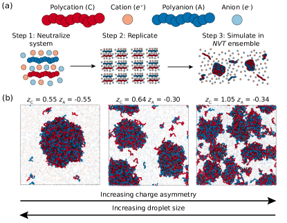
Figure 1: MD simulations show smaller droplets for larger charge asymmetry.
(a) Schematic of simulations set-up, where a system of two oppositely charged polyions is neutralized with counterions, replicated, and simulated in the ensemble (i.e., constant number of particles, volume, and temperature).
(b) Snapshots from three simulations at various charge pairings of the polycation (, red) and polyanion (, blue) showing that larger charge asymmetry leads to smaller droplets.
For clarity, counterions are shown 99% transparent.
To investigate the influence of charge asymmetry on phase separation, we first performed molecular dynamics (MD) simulations of a system consisting of polycations , polyanions , and the respective counterions, and (Fig. 1a).
For simplicity, we kept the length of the polyions fixed at ten times the size of an ion and instead varied the respective charge numbers per monomer, and , to study different charge asymmetries .
We ensured charge neutrality of the entire system by compensating each charge on polyions by respective counterions.
We modeled the direct interactions between oppositely charged polyions by attractive Lennard-Jones interactions and used excluded volume interactions between all other species.
Additional details are described in the Appendix.
The snapshots of equilibrated MD simulations shown in Fig. 1b demonstrate that polyions form dense droplets surrounded by a dilute phase.
Importantly, we find smaller droplets for larger charge asymmetry, indicating that droplet size is controlled and multiple droplets can stably coexist.
To reveal the physical mechanism of the observed droplet size regulation, we next describe the system using a continuous field theory.
Here, the state of the incompressible, isothermal mixture is captured by the volume fraction fields , , , and of the charged species.
The remaining fraction, (here and below sums are over the four species , , , and ), is filled by an inert solvent .
The system’s equilibrium is governed by the minimum of the total free energy , where the terms respectively capture local, interfacial, and long-ranged electrostatic interactions akin to Ref. [13].
We approximate local interactions using the Flory–Huggins model [22, 23],
(1)
where integrals are over the system of volume , is the relevant thermal energy scale, and denotes the molecular volume, where solvent molecules, ions, and monomers of the polyions have the same volume for simplicity.
In the integrand, the first term proportional to the Flory parameter accounts for attraction between polycations and polyanions , whereas the other terms capture translational entropies.
To mimic the MD simulations, we chose the respective chain lengths as and .
In contrast, the interfacial energy is described by
(2)
which limits the width of interfaces between coexisting phases to roughly in strongly interacting systems [24].
Finally, long-ranged electrostatic effects are captured by the electrostatic potential , which is governed by the free energy
(3)
where is the dielectric constant, which we assumed to be spatially invariant.
The charge numbers represent the degree of ionization of each monomer, in units of the elementary charge , so the charge asymmetry is .
Taken together, the equilibrium state thus depends on the local attraction (), the interfacial penalty (), and the charge numbers ( and ).
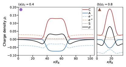
Figure 2: Field theory predicts droplet-like periodic patterns.
Periodic profiles of charge density for all species and total charge density as a function of distance for weak (left) and strong (right) charge asymmetry .
Parameters are , , , , , and , with Bjerrum length .
To mimic the MD simulations, we impose constant average fractions with .
To ensure global charge neutrality, we set and adjust the fraction of counterions, and .
Based on the results shown in Fig. 1b, we expect that equilibrium states exhibit droplets of a well-defined size, which corresponds to periodic profiles in the field theory.
To describe such states, we for simplicity consider a one-dimensional, periodic system of length , and minimize by varying , , and .
Here, we allow for coexisting phases with different periods and we impose mass conservation, incompressibility, and charge neutrality within each phase using Lagrange multipliers, akin to Ref. [25] and described in the Appendix.
The resulting equilibrium profiles shown in Fig. 2 indicate that the field theory indeed predicts periodic patterns, where regions of large polyion density correspond to the droplets and the surrounding region enriched in counterions represent the dilute phase.
However, the counterions do not neutralize the system everywhere (black line), which we confirmed in MD simulations (Fig. S1 in the Appendix).
These net charges are reminiscent of the double layer structure reported for complex coacervates [26] and indicate that electrostatics are crucial for droplet size control [11].
Indeed, we observe larger periods for smaller charge asymmetry (Fig. 2), consistent with the larger droplets in the MD simulations (Fig. 1b).
There are also subtle differences between the two panels: For small charge asymmetry (Fig. 2a), the charge density exhibits a dip inside the droplet and reaches neutrality () in the dilute phase.
Both effects are absent for larger charge asymmetry (Fig. 2b), suggesting that these two cases are qualitatively different.
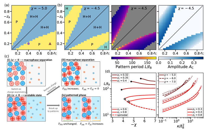
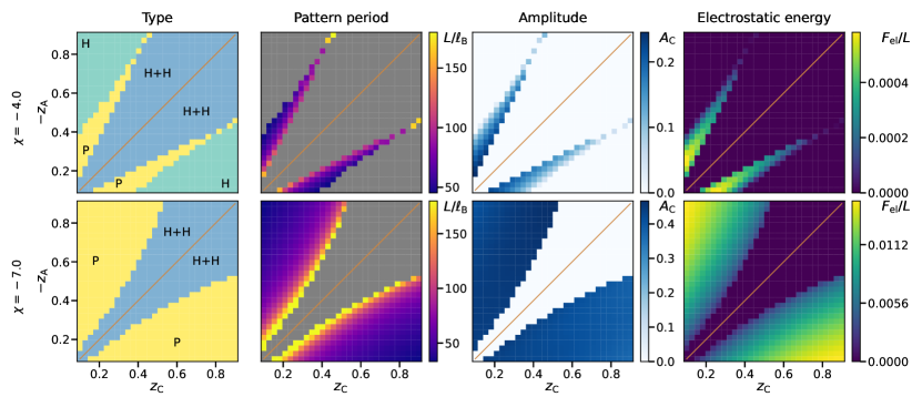
Figure 3: Field theory predicts transitions to patterned phases.
(a) Phase diagram as a function of the charge numbers of polycations () and polyanions () revealing parameter regions with the coexistence of two homogeneous phases (H+H) and patterned phases (P) for strong attraction (). The colored markers correspond to the two panels in Fig. 2.
(b) Phase diagram for weak attraction () including regions with a single homogeneous phase (H).
The remaining columns show respective periods and amplitudes of the polycation profile.
(c) Schematic explanation of the origin of the patterned phase.
The initial phase-separated charge-neutral state in (i) is destabilized due to net charges if charge asymmetry is enabled in (ii).
An equilibrium state can either be reached by restoring charge neutrality in (iii) or by breaking the phases into smaller droplets in (iv).
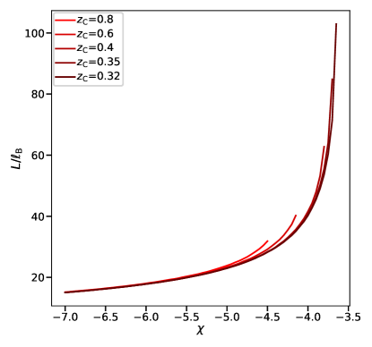
(d) Pattern length scale as a function of interaction parameter (left, interfacial parameter ) and (right, various ) for various at .
As decreases, the patterned phase transitions to macrophase separation (stars) or a homogeneous state (open disk).
Dashed lines indicate the most unstable length scale predicted by the linear stability analysis in the Appendix.
(a–d) Additional parameters are given in Fig. 2.
We next analyze in detail how the periodic patterns depend on the charge numbers and .
Fig. 3a shows that periodic patterns only appear in a restricted parameter region (yellow region P).
In particular, the patterned phase does not exist for symmetric mixtures (diagonal line, ).
Instead, the system exhibits macrophase separation (blue H+H region) if is sufficiently negative, and this region becomes larger for weaker interactions (Fig. 3b and Fig. S6 in the Appendix.)
Moreover, the system stays homogeneous for very asymmetric mixtures (teal H region).
Taken together, these observations suggest periodic patterns emerge for sufficiently strong attraction (large ) and intermediate charge asymmetry between polyions.
We can understand the emergence of patterned phases starting from the charge-balanced state (, Fig. 3c, subpanel (i).
In this case, the polyions form a dense macrophase while the small molecules (, , and ) accumulate in the corresponding dilute phase.
Here, we have since and the energy of the single interface is negligible in a thermodynamically large system.
Switching on charge asymmetry (, subpanel (ii) destabilizes this state because the macrophases acquire a net charge, so the electrostatic energy diverges.
To minimize the total free energy , the state can change in two fundamentally different ways: it can either restore charge neutrality (subpanel iii) or form a patterned phase (subpanel iv).
In the first alternative, counterions move into the dense phase (maintaining macrophase separation, subpanel (iii), which restores charge neutrality and maintains .
However, the small counterions decrease the concentration of polyions, thus reducing their contact and increasing .
In the second alternative, the dense phase is broken up to form a pattern of finite length scale (subpanel iv).
In the simplest case, the polyions maintain a high concentration, implying that changes negligibly.
However, the electrostatic energy is now finite, and the breakup creates many interfaces, so both and are positive.
Taken together, both alternatives increase compared to the neutral initial case, but breakup into the patterned phase is favored for strong attraction (large negative ).
The preceding argument also makes qualitative predictions for the pattern period as a proxy for droplet size.
Assuming stays roughly constant in the patterned phase, will depend only weakly on and is instead governed by the minimum of .
Generally, decreases with increasing (since there are fewer interfaces per unit length), whereas increases with (since opposite charges are separated further for larger , i.e., exchanging the two central slabs in Fig. 3c(iv) costs electrostatic energy).
These arguments predict that increases with larger (increasing ), whereas decreases with larger (increasing ).
We present a more quantitative argument in the Appendix, which shows that at the free energy minimum the two energies have opposing dependencies on , , leading to a trade-off where at the minimum.
We thus generally expect that increases with larger and smaller .
We test our predictions by analyzing the patterned phases obtained from the field theory.
Fig. 3b shows that indeed decreases for larger (away from the symmetry line), although the patterns completely vanish for large where the homogeneous state exhibits the lowest free energy.
The right-most panel in Fig. 3b shows that the amplitude of decreases with increasing , implying that polyions become less concentrated.
This is not captured by the simple argument above, suggesting that the system compromises the segregation of polyions (implying larger ) for a lower electrostatic energy .
Indeed we find that exhibits a non-monotonous dependency on (Fig. S11 in the Appendix), and the patterns cease when vanishes.
Concomitantly, the amplitude approaches zero (Fig. 3b), suggesting that the transition to the homogeneous phase is continuous.
To also test the influence of the interaction strength and the interfacial parameter , we performed additional minimizations.
Fig. 3d confirms a weak influence of , whereas increases significantly with .
Note that the length scale predicted from the most unstable perturbation around the homogenous state (dashed line in Fig. 3d; details in the Appendix) generally does not predict the equilibrium periods.
However, both values coincide at the transition of the patterned phase to the homogeneous state (open circles) and the scaling is consistent with mean-field theory (Fig. S5 in the Appendix), supporting that this is a continuous phase transition.
Taken together, the numerical solutions of the field theory confirm that (and thus the droplet size) increases with larger and smaller , while has a minor influence beyond driving phase separation in the first place.
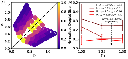
Figure 4: MD simulations corroborate field theory. (a) Simulations at various charge numbers (, ) demonstrate that high charge asymmetries result in smaller average droplet sizes (normalized by total number of polyion chains in the system). (b) Normalized droplet size as a function of attraction strength .
Decreasing mildly increases or decreases droplet size depending on charge asymmetry.
To test whether our predictions hold more generally, and in particular in 3D systems, we return to our MD simulations (details described in the Appendix).
Fig. 4a shows that larger charge asymmetry indeed leads to smaller droplets.
We also observe system spanning droplets close to charge neutrality (; yellow symbols), which are consistent with macrophase separation (region H+H in Fig. 3).
The detailed size distributions shown in Fig. S2 in the Appendixindicate this dependence unambiguously, although finite size effects are clearly visible for small charge asymmetries.
Moreover, Fig. 4b shows that varying the interaction strength between the polyions affects the droplet size only weakly, consistent with the weak influence of shown in Fig. 3d.
In both cases, at weak charge asymmetry droplet size slightly decreases for larger attraction, conversely to the behavior at strong charge asymmetry.
Taken together, these data confirm the predictions from the field theory, suggesting that droplet size control by net charges is a general phenomenon.
The described droplet size control essentially emerges from a trade-off between short-ranged attraction driving phase separation and long-ranged electrostatic repulsion if droplets accumulate net charges.
At weak charge asymmetry, the system exhibits macrophase separation since the attraction dominates.
Conversely, for strong charge asymmetry, the system will stay homogeneous to avoid accumulating net charges.
Between these two extremes, the patterned phases emerge as a compromise between phase separation and accumulating net charge.
This behavior is reminiscent of phase separation in elastic media, where elastic effects mediate long-ranged repulsion, resulting in patterned phases and a continuous transition to the homogeneous state [25].
This similarity suggests that droplet size can be generally controlled when the short-ranged attraction leading to phase separation is opposed by some long-ranged repulsion, reminiscent of classical pattern formation [27].
Another example for this mechanism are chemically active droplets, where long-ranged repulsion emerges from a reaction-diffusion system [28, 29, 24, 30], which can in fact be interpreted using an electrostatic analogy [31, 32, 33].
Here, we focused on the most basic mechanism of droplet size control by net charges.
For instance, we assumed that polyions have a fixed charge, whereas realistic molecules will exhibit charge regulation, so their behavior will depend on pH.
Molecules involved in complex coacervation, and particularly in biomolecular condensates, are also much more complex: their charge distribution will be inhomogeneous, the unspecific interactions will be heterogeneous and might depend on charge, and the polymer structure cannot be ignored, particularly for nucleic acids and intrinsically disordered protein regions [34].
It will be interesting to see how such effects influence the described size control and how these charge asymmetries affect condensates inside cells.
It is already tempting to speculate that charged droplets were implicated in the origin of life [35, 36], so that their size is maintained and the associated Rayleigh instability [18, 17] could explain division.
Acknowledgements
We thank Jan Kirschbaum for stimulating discussions, and we thank Nynke Hettema, Noah Ziethen and Athanassios Panagiotopoulos for helpful comments on our manuscript.
We gratefully acknowledge funding from the Max Planck Society and the European Union (ERC, EmulSim, 101044662), the Chan Zuckerberg Initiative DAF (an advised fund of Silicon Valley Community Foundation; grant 2023-332391 ), and departmental start-up funds via the Department of Chemical and Biological Engineering and the Omenn–Darling Bioengineering Institute at Princeton University. This research was partially supported by the National Science Foundation (NSF) through the Princeton University (PCCM) Materials Research Science and Engineering Center DMR-2011750.
References
Banani et al. [2017]S. F. Banani, H. O. Lee,
A. A. Hyman, and M. K. Rosen, Nat. Rev. Mol. Cell Biol. 18, 285 (2017).
Dignon et al. [2020]G. L. Dignon, R. B. Best, and J. Mittal, Annu. Rev. Phys.
Chem. 71, 53 (2020).
Zhou and Pang [2018]H.-X. Zhou and X. Pang, Chem. Rev. 118, 1691 (2018).
Meyer et al. [2024]K. Meyer, K. Yserentant,
R. Cheloor-Kovilakam,
K. M. Ruff, C.-I. Chung, X. Shu, B. Huang, and O. D. Weiner, bioRxiv (2024).
Sing and Perry [2020]C. E. Sing and S. L. Perry, Soft
Matter 16, 2885
(2020).
Pak et al. [2016]C. W. Pak, M. Kosno, A. S. Holehouse, S. B. Padrick, A. Mittal, R. Ali, A. A. Yunus, D. R. Liu, R. V. Pappu, and M. K. Rosen, Molecular Cell 63, 72 (2016).
Lyons et al. [2023]H. Lyons, R. T. Veettil,
P. Pradhan, C. Fornero, N. De La Cruz, K. Ito, M. Eppert, R. G. Roeder, and B. R. Sabari, Cell 186, 327 (2023).
Chang et al. [2017]L.-W. Chang, T. K. Lytle,
M. Radhakrishna, J. J. Madinya, J. Vélez, C. E. Sing, and S. L. Perry, Nature Communications 8, 1273 (2017).
Ziethen and Zwicker [2024]N. Ziethen and D. Zwicker, J.
Chem. Phys. 160, 224901
(2024).
Liu and Goldenfeld [1989]F. Liu and N. Goldenfeld, Phys. Rev. A 39, 4805
(1989).
Holehouse and Kragelund [2023]A. S. Holehouse and B. B. Kragelund, Nat. Rev. Mol. Cell Biol. (2023).
Oparin [1938]A. I. Oparin, The Origin of Life (Dover Publications, Inc., New York, 1938).
Brangwynne and Hyman [2012]C. P. Brangwynne and A. A. Hyman, Nature 491, 524
(2012).
Stukowski [2010]A. Stukowski, MODELLING AND
SIMULATION IN MATERIALS SCIENCE AND ENGINEERING 18, 10.1088/0965-0393/18/1/015012 (2010).
Qiang et al. [2024b]Y. Qiang, C. Luo, and D. Zwicker, arXiv preprint
arXiv:2405.01138 (2024b).
Appendix A Details of the molecular dynamics (MD) simulations
A.1 Simulation procedure
Molecular dynamics simulations are run in the ensemble with neutral mixtures of polyions and counterions in implicit solvent (Fig. 1) using Lennard-Jones units. All particles are modeled with a size and a mass . The total energy of the simulation system is given by:
(S1)
where describes the long-range electrostatic interactions between charged monomers, describes the same chain bonded interactions and short-range heterotypic attraction between polycations and polyanions , and describes the ion-ion, ion-polymer, and homotypic polymer-polymer excluded-volume interactions. More specifically, is modeled using Coulomb’s potential:
(S2)
In this form, describes the type of the charged monomers and , is the distance between the charged monomers, and the dielectric constant is . Next, models the combination of the bonded potential and the Lennard-Jones potential with cut-off and shifting:
(S3)
Here, is total number of polymers in the system, is the polymer length. The bonded potential is modeled using a harmonic potential . As for the Lennard-Jones potential we use:
(S4)
Finally, for the excluded volume for all the particles (besides interactions between and ), we use the Weeks-Chandler-Andersen (WCA) potential
(S5)
In all simulations, we use polyions and each polyion is composed of bonded monomers.
We use a bond coefficient of and an equilibrium distance . For the Lennard-Jones interactions, we use a cut-off of and attraction strength of which is also the energy scale for other interactions. The charge of polyions are varied by simulation. The charge of counterions are set to have a magnitude of . Electrostatic interactions are calculated using a PPPM grid for interactions beyond . Electrostatic interactions within are calculated directly. The dielectric constant is set to . The volume fractions of each species in the simulation box are set to be and and .
Each simulation trajectory is first annealed at a temperature of for using a Langevin thermostat with a damping of . Thereafter, the temperature of each simulation is set to also using a Langevin thermostat with a damping of . Simulation trajectories are then run for million . The last million is collected for data analysis, sampling a frame every . We use a timestep of in the simulations.
Further, in the analysis of MD simulations, droplets are defined using a cutoff of between polyions. The trajectory analysis software Ovito [37] is used to generate cluster data from simulation frames. An in-house code is used to generate radial density profiles from an Ovito [37] cluster analysis pipeline.
A.2 Additional result figures
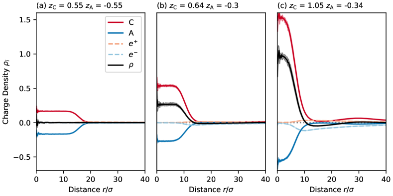
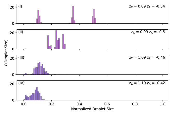
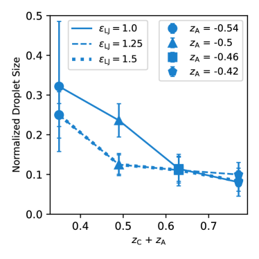
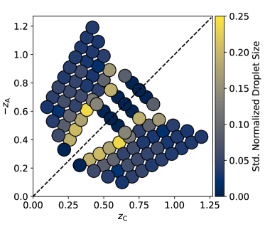
Additional figures are presented in this section corresponding to results from MD simulations. Figure S1 presents radial charge density profiles from MD simulations at (, ), (, ), and (, ). See Fig. 1 for a visualization of these droplets. Figure S2 shows normalized droplet size distributions corresponding to the four data points in Fig. 4a. Figure S3 confirms that the relationship between charge asymmetry and droplet size holds across three different values of . Finally, Figure S4 quantifies the standard deviations in normalized droplet sizes for the simulations presented in Fig. 4a.
Figure S1: Radial charge density profiles indicate charge asymmetry controls droplet size. Radial charge density profiles (RDPs) for (a) , (b) , and (c) , . Shaded regions indicate plus and minus the standard deviation from three equal blocks of the 1,000 frames used in generating the RDPs. The profiles indicate that increasing charge asymmetry decreases droplet size. See Fig. 1 for visualization of these droplets.Figure S2: Larger charge asymmetries create broader distributions of droplet size. Four simulation systems, (I) , (II) , (III) , (IV) , , corresponding to Fig. 4a are plotted in histograms of normalized droplet sizes. At larger charge asymmetries (III and IV), the distribution of cluster sizes is larger and the average droplet size is smaller. Finite-sized effects prevail at smaller charge asymmetries (I and II) indicated by the multi-modal distributions (i.e., size discrepancy among sustained droplets).Figure S3: Charge asymmetry’s effect on droplet size is preserved at higher polyion attraction strengths. The normalized droplet size for four charge pairings ((, ), (, ), (, ), (, ) corresponding to I-IV in Fig. 4a) at three different attraction strengths between oppositely charged polyions (). As charge asymmetry is increased the normalized droplet size in the simulations decreases regardless of the value of . Error bars represent standard deviation in the droplet size data at every condition.Figure S4: Error on simulation droplet sizes indicate finite-sized effects. The standard deviation in the normalized droplet sizes plotted in Fig. 4a for each simulation. Larger standard deviation (yellow) for moderate charge asymmetries are likely due to finite-sized effects resulting in size discrepancies among sustained droplets (see Fig. S2).
Appendix B Details of the field theory
The main idea of the solution of the field theory defined in the main text is to separate the entire system into different phases, which each can either be homogeneous or exhibit periodic patterns.
Periodic patterns are described by the fields over one period together with the period along each of the space dimensions.
B.1 Free energy minimization
We consider a -dimensional incompressible, isothermal mixture composed of components with charge numbers for .
The total free energy including local, interfacial, and long-ranged electrostatic interactions reads
(S6)
Using the Bjerrum length , , , , , and , we obtain the dimensionless free energy density ,
(S7)
To study the coexistence of different phases, we consider a Gibbs ensemble of phases, where the fraction of volume of phase is , implying .
The average free energy density of the entire system reads
(S8)
Additionally, there are several constraints, including mass conservation for each species,
(S9)
incompressibility everywhere in each phase,
(S10)
and charge neutrality in each phase,
(S11)
Using these constraints, the equilibrium coexisting states can be obtained by minimizing over , , , and the vector describing the size of the compartment in all dimensions, which can be different in each phase.
To alleviate the problem of negative volume fractions during the relaxation dynamics and conserve the average volume fractions, we replace the logarithms associated with the translational entropies by introducing conjugated fields , akin to [38].
This leads to the extended average free energy density
(S12)
where
(S13)
Here, are the conjugate fields of , whereas , , and are the Lagrange multipliers for incompressibility, compartment volume conservation, and charge neutrality, respectively. The last term with a constant is added to guide the convergence to charge neutrality, which is zero when fully convergent.
The extremum of the free energy density with respect to provides
(S14)
which gives
(S15)
Note that this automatically satisfies material conservation,
(S16)
Inserting Eq. (S15) together with the constraints into the free energy density gives exactly except for a constant offset , demonstrating the extremum of is equivalent to the extremum of , which we want to calculate.
The extremum of with respect to provides
(S17)
The extremum of with respect to results in the electrostatics Poisson’s equation
(S18)
The extremum of with respect to provides
(S19)
The extremum of with respect to gives charge neutrality in each compartment,
(S20)
The extremum of with respect to and simply gives incompressibility and volume conservation constraints,
(S21)
and
(S22)
respectively.
The extremum of with respect to , the -th component of , gives
(S23)
where the star means that quantities are evaluated for profiles that have been obtained by optimizing over all fields and parameters except .
In particular, denotes the associated free energy density, which then only depends on .
Using and ,
we obtain
(S24)
which gives
(S25)
Using Poisson’s equation and integration by parts, we find
(S26)
and thus for all compartments.
This indicates that the electrostatic energy is balanced by the interfacial energy in equilibrium.
Specifically, in the 1D case, we have
(S27)
In summary, we obtain the self-consistent equations (S13), (S15),
(B.1)–(S22),
and (S24) to determine equilibrium states.
B.2 Numerical minimization method
We designed an iterative scheme based on the self-consistent equations above, where we update all values of fields and variables based on their current approximated values, so the iteration converges to the free energy minimum.
In this scheme, we first calculate using Eq. (S13), and using Eq. (S15).
We then calculate via
(S28)
where is the wavenumber of the Fourier transform and its inverse .
Next, we calculate using Eq. (B.1) and the incompressibility condition given by Eq. (S21),
(S29)
We now use Eq. (B.1) to update the ideal part of the new field, , via
(S30)
To ensure numerical stability, we update the new field using a mixture of the old and the ideal one together with the kernel ,
(S31)
where is an empirical acceptance rate, typically around .
We next use Eq. (B.1) to update . More specifically,
using
(S32)
and
(S33)
we update via
(S34)
Here, is another empirical acceptance rate, which is typically set to 0.001. Afterwards, we shift to satisfy Eq. (S22) which reads .
Next, we update using Eq. (S20),
(S35)
where is the third acceptance rate, which is set to .
Finally, in 1D, we update using Eq. (S27), via
(S36)
where is an empirical acceptance rate around .
We use this iterative scheme to find the equilibrium states, where each phase is described by fields and together with optimized sizes .
To produce the results of the main text, we use , assume , and discretize fields at points along the one dimension.
We have checked the correctness at selected parameter values by using ; All convergent results are consistent with those using .
B.3 Linear stability analysis
We here present the linear stability analysis for the uniform state .
We perturb by a small value, setting , where is the perturbation amplitude and is the associated wave number. By evaluating Eq. (S7), taking the second-order derivative of with respect to , and then taking the limit , we obtain the Hessian matrix
(S37)
For the homogeneous state to be stable, all eigenvalues of the Hessian matrix must be positive for all .
If the homogeneous state is unstable, we numerically calculate the eigenvalues and identify the lowest as a function of .
The length scale of this most unstable mode is given by and shown in Fig. 3d of the main text.
We also show the most unstable length scale for small charge asymmetry in Fig. S5, indicating that this length strongly depends on , while the charge asymmetry has a weak effect, in contrast to the results for the equilibrium length scale.
Figure S5:
The most unstable length scale predicted from linear stability analysis. Parameters are the same as in Fig. 3(d) of the main text.
B.4 Additional result figures
Figure S6 shows phase diagram of states, pattern periods, amplitudes, and electrostatic energy for and , analogous to Fig. 3b in the main text. Figures S7 and S8 provide additional details for states depicted in Fig. 2 of the main text. Figure S9 shows a typical profile near the continuous transition. This transition is demonstrated by the amplitude of the polycation volume fraction, as shown in Fig. S10. The different contributions to the free energy are shown in Fig. S11. The last two columns, in particular, demonstrate that the interfacial energy is equal to the electrostatic energy .
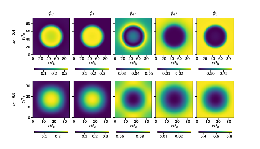
We also obtain the patterned phase by solving the two-dimensional mean-field theory equations. We show the profiles of volume fractions in Fig. S12 and charge densities in Fig. S13, corresponding to the same states as in Fig. 2 of the main text. The 2D disk patterns qualitatively agree with the 1D results; notably, we also observe a dip inside the droplet at .
Figure S6:
Results analogous to Fig. 3 in the main text for (upper row) and (lower row).
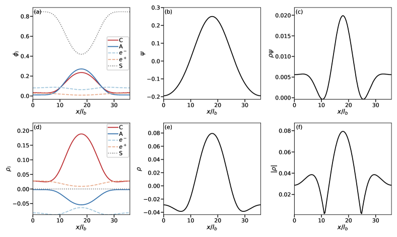
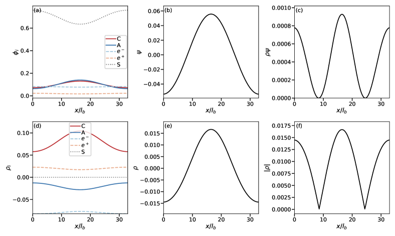
Figure S7:
Additional details for the state for weak charge asymmetry shown in Fig. 2a in the main text.
Parameters are , , , and .
(a) Volume fractions .
(b) Electrostatic potential .
(c) Local electrostatic energy density .
(d) Charge density for each species.
(e) Total charge density .
(f) Absolute value of total charge density.
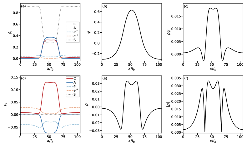
Figure S8:
Additional details for the state for weak charge asymmetry shown in Fig. 2b in the main text.
Parameters are , , , and .
(a) Volume fractions .
(b) Electrostatic potential .
(c) Local electrostatic energy density .
(d) Charge density for each species.
(e) Total charge density .
(f) Absolute value of total charge density.
Figure S9:
Typical profile close to continuous transition.
Parameters are , , (the critical point is at ), and .
(a) Volume fractions .
(b) Electrostatic potential .
(c) Local electrostatic energy density .
(d) Charge density for each species.
(e) Total charge density .
(f) Absolute value of total charge density.
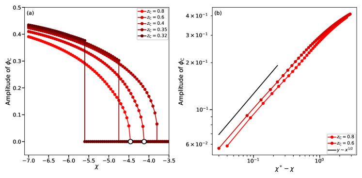
Figure S10: Amplitude decreases as increases. (a) The amplitude of polycation profile decreases as increases. The circle indicates the critical point at where for and for . (b) Scaling of the amplitude as a function of the relative interaction strength . The exponent is consistent with the critical exponent in mean-field theory, indicating that the transition is continuous.
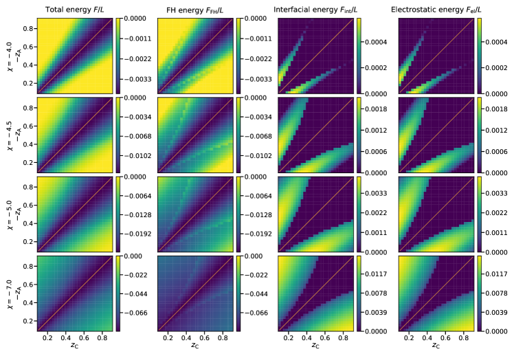
Parameters are and . Remaining parameters are the same as in Fig. 2 in the main text.Figure S11: Different contributions to the free energy.
Total energy density , and its three contributions , , and , normalized to the size as a function of the charges and of the polyions for various interaction strengths .
To highlight the details and have been shifted by the free energy ) of the respective homogeneous states.
Consistent with Eq. (S26), and are always identical.
Figure S12:
Two-dimensional profiles of the volume fractions predicted by the field theory. The parameters are the same as in Fig. 2 of the main text.
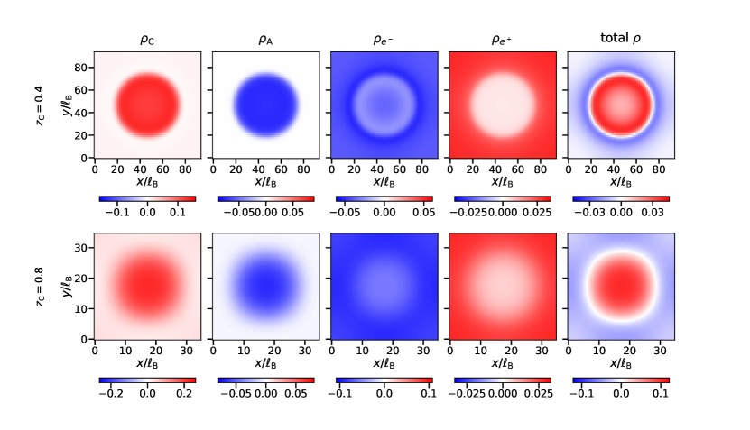
Figure S13:
Two-dimensional profiles of the charge densities, , predicted by the field theory. The last column shows the total charge density, .