Higher-criticism for sparse multi-sensor change-point detection

Abstract

We present a procedure based on higher criticism [9] to address the sparse multi-sensor quickest change-point detection problem. Namely, we aim to detect a change in the distribution of the multi-sensor that might affect a few sensors out of potentially many while those affected sensors, if they exist, are unknown to us in advance. Our procedure involves testing for a change point in individual sensors and combining multiple tests using higher criticism. As a by-product, our procedure also indicates a set of sensors suspected to be affected by the change. We demonstrate the effectiveness of our method compared to other procedures using extensive numerical evaluations. We analyze our procedure under a theoretical framework involving normal data sensors that might experience a change in both mean and variance. We consider individual tests based on the likelihood ratio or the generalized likelihood ratio statistics and show that our procedure attains the information-theoretic limits of detection. These limits coincide with [7] when the change is only in the mean.

1 Introduction

Sequential change-point detection, which aims to quickly identify changes in the distribution of streaming data, has long been a fundamental challenge in statistics [30]. Recently, there has been much interest in high-dimensional settings where changes affect only a small subset of variables, a scenario referred to as sparse multi-sensor change-point detection [31, 8, 7, 14, 16, 24]. The challenges in this situation are the relatively small number of affected sensors whose identity is unknown to us in advance, and the generally weak change in distribution each affected sensor might experience. In offline hypothesis testing, Higher Criticism (HC) [9] has proven to be an effective tool for global testing against sparse alternatives [12]. Despite the clear connection between HC and sparse change-point detection, its adaptation to the sequential detection framework, where decisions are made in real time, remains underexplored.

In this paper, we bridge this gap by developing a new sequential change-point detection procedure that applies HC to combine individual sensors’ test statistics. Our method is based on large-scale inference techniques, particularly suited for sparse and weak signals. By aggregating P-values from individual change-point tests, our approach is sensitive to changes that affect only a small fraction of the sensors, even when the identities of the affected sensors are unknown. Since the procedure wraps around P-values without assuming parametric form of pre- and post-change distributions or assuming distributions of P-values, our HC procedure is flexible and enables distribution-free detection statistics. Moreover, HC provides a mechanism to identify sensors suspected to be affected, offering optimality properties compared to other feature selection methods, such as the Benjamini-Hochberg procedure for controlling the false discovery rate [10, 11]. We demonstrate the effectiveness of our method through extensive numerical evaluations and provide a theoretical analysis under a normal multi-sensor setting, where sensors may experience changes in both mean and variance. Our results show that our procedure attains the information-theoretic limits of detection, coinciding with the results in [7] when only the mean is affected.

Our work builds upon recent advancements in multi-sensor data analysis [15, 22, 24, 28], particularly in the context of sequential change-point detection [8, 5, 30], providing a robust and theoretically justified approach for detecting sparse changes in high-dimensional data. But our work differs and offers the following key contributions:

• We propose a sequential change-point detection method based on Higher Criticism, effectively detecting global changes while identifying sensors suspected to be affected.

• We derive the asymptotic detection delay of HC of $\mathsf{LR}$ or $\mathsf{GLR}$ P-values under a Gaussian multi-sensor model with a potential sparse change in means and variances, where individual tests use the likelihood ratio (LR) based CUSUM and the generalized likelihood ratio (GLR).

• We characterize the asymptotic information theoretic detection delay under the model mentioned earlier ([7] characterized the expected detection delay in the homoscedastic case using LR). Our result shows that the detection delay of HC of $\mathsf{LR}$ or $\mathsf{GLR}$ P-values asymptotically equals the information-theoretically optimal detection delay.

These results indicate that HC based on either $\mathsf{LR}$ or $\mathsf{GLR}$ is adaptive to the rarity level, the post-change mean intensity, and the change in variance.

The rest of the paper is organized as follows. Section 2 sets up the problem. Section 3 presents the HC procedure for sequential change-point detection. Section 4 contains the main theoretical results. Section 5 contains numerical examples that validate the theory and compare with other methods. Section 6 summarizes the paper. Section 7 contains proofs. Some proof details are delegated to the Appendix.

2 Problem setup

Assume $N$ sensors, and for the $n$th sensor, we observe a sequence of observations $X_{n,t}$, $t=1,2,\ldots$. The null hypothesis states no change in the distribution of the sequence. Under the alternative hypothesis, there exists an unknown change point $\tau$, $0<\tau<\infty$, and an unknown subset of sensors with index set $I$ of $\{1,\ldots,N\}$ affected by the change and thus their distribution changes for $t=\tau,\tau+1,\ldots$. In contrast, the distribution of each unaffected sensor remains unchanged. More formally, we are testing the hypothesis sequentially:

$$H_{0}: \quad X_{n,t}\sim F_{0n},t=1,2,\ldots$$ (1)

$$H_{1}: \quad X_{n,t}\sim F_{0n},t=1,\ldots,\tau-1,$$ (2)

$$\quad X_{n,t}\sim F_{1n},t=\tau,\tau+1,\ldots,n\in I,$$ (3)

$$\quad X_{n,t}\sim F_{0n},t=1,2,\ldots,n\notin I.$$ (4)

Our goal is to find a detection procedure, typically a stopping rule, that can detect the change as quickly as possible after it occurs while allowing a sufficiently large average-run-length (ARL) when there is no change.

We focus on the sparse change case in which the fraction of affected sensors $p:=|I|/N$ is small. Our approach involves testing for a change in every sensor individually and combining multiple tests using higher-criticism [9, 12].

3 Detection procedure using Higher Criticism

Given the observations at time $t$, suppose we use certain detection statistics $Y_{n,t}$ that is a function of $\{X_{n,s}\}_{s\leq t}$. For each sensor $n$, we compute a P-value of $Y_{n,t}$ with respect to the no-change distribution $F_{0n}$. Let $\{\pi_{n,t}\}$, $n=1,\ldots,N$ be a sequence of P-values at time $t=1,2\ldots$.

Before presenting the procedure, we first review the Higher Criticism (HC) statistic studied in [9, 12]. For a given collection of P-values $\pi_{1},\ldots,\pi_{N}$, let $\pi_{(1)}\leq\cdots\leq\pi_{(N)}$ be their ordered version. HC statistic of a collection of P-values is defined as

$$\mathrm{HC}^{\star}(\pi_{1},\ldots,\pi_{N}):=\max_{1\leq n\leq\alpha_{0}N}\sqrt{N}\frac{\frac{n}{N}-{\pi}_{(n)}}{\sqrt{\frac{n}{N}\left(1-\frac{n}{N}\right)}},$$ (5)

where $\alpha_{0}\in(0,1)$ is a tunable parameter known to have little effect on the large sample behavior of $\mathrm{HC}^{\star}$ [12]. To apply HC in the sequential setting, we form the detection statistic at time $t$

$$\mathrm{HC}^{\star}_{t}=\mathrm{HC}^{\star}(\pi_{1,t},\ldots,\pi_{N,t}),\qquad t=1,2\ldots.$$ (6)

We detect a change when the sequence $\{\mathrm{HC}_{t}^{\star}\}_{t=1,2,...}$ exceeds a prescribed threshold sequence $\{b_{t}\}_{t=1,2,...}$ for the first time. This detection procedure corresponds to the following stopping rule called the HC procedure

$$T=\inf\{t>0:\mathrm{HC}_{t}^{\star}>b_{t}\},$$ (7)

where $b_{t}>0$ is a user-specified (usually time-invariant) threshold chosen to control the probability of false alarm when there is no change, and thus control the Average Run Length (ARL). Figure 1 presents an example of the detection statistic and their empirical distributions before and after the change.

When the detection statistic has exceeded the threshold thus a change has been declared, we may select sensors suspected to experience a change using HC thresholding [10, 11]. Prior works [10, 11, 12] discuss this selection mechanism and show that it has interesting optimality properties in the context of feature selection for inference.

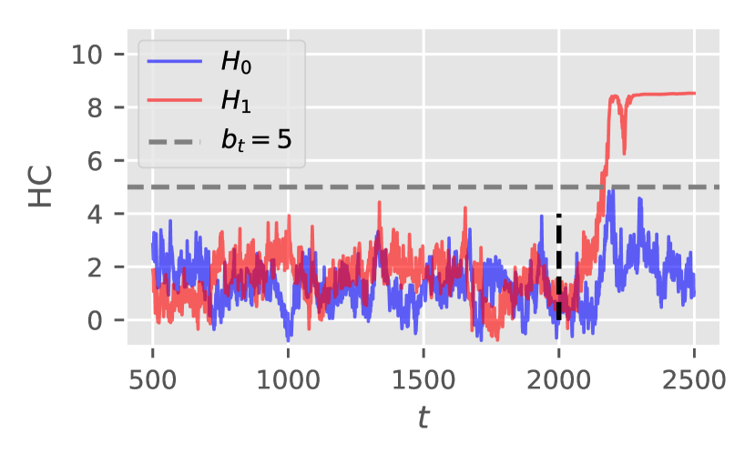
Figure 1: Realizations of the Higher Criticism (HC) detection statistic $\mathrm{HC}^{\star}_{t}$ of (6) over $t$ under either hypothesis with $N=500$. P-values on each sensor are computed from CUSUM procedures. Under $H_{1}$, $\mathrm{HC}_{t}^{\star}$ are for the normal mean-shift problem changing from $\mathcal{N}(0,1)$ to $\mathcal{N}(0.35,1)$ with $|I|=4$. The true change-point occurs at $\tau=2000$.

4 Asymptotic detection delay under sparse changes

We analyze the performance of the HC procedure under a normal means model with sparse and weak location shifts and potential heteroscedasticity. Namely, in the notation of (1), observations are independent, $F_{0n}=\mathcal{N}(0,1)$ and $F_{1n}=\mathcal{N}(\mu,\sigma^{2})$, for all $n=1,\ldots,N$. Here $\mu\geq 0$ is the common shift in the means of all affected sensors and $\sigma>0$ is associated with a common change in their variances. The homoscedastic case ($\sigma=1$) corresponds to the setting of [8, 7, 16]. We will consider an asymptotic setting in which the number of sensors $N$ tends to infinity while the sparsity parameter $p$ and the intensity of the change are calibrated to $N$ similarly to [7].

We consider two useful examples of test statistics in individual sensors. We drop the dependence on the sensor index for notational simplicity.

Example I: CUSUM for mean-shift (see, e.g., [23]). Consider the CUSUM statistic formed on each sensor assuming the known post-change mean:

$$Y_{t}^{\mathsf{LR}} :=\max_{k\leq t}V_{t,k},\qquad V_{t,k}:=\left(S_{t}-S_{k}-\frac{\mu}{2}(t-k)\right)\mu,$$ (8)

where $S_{t}:=\sum_{j=1}^{t}X_{j}$, and $\mu$ is the assumed post-change mean. Note that this is associated with the likelihood ratio statistic for change in the mean of a normal model from zero to $\mu_{N}(r)$ while the variance is unchanged. This statistic arises in testing for a mean shift by $\mu$ under local asymptotically normal family; see the discussions in [29, 30] and references therein. The CUSUM $Y_{t}^{\mathsf{LR}}$ can be computed recursively in time $t$, facilitating its online implementation and thus a popular choice for online change-point detection. P-value corresponds to the survival function of $Y^{\mathsf{LR}}_{t}$ and is given by

$$\pi_{t}^{\mathsf{LR}}(x) :=\Pr\left[Y_{t}^{\mathsf{LR}}\geq x|H_{0}\right].$$ (9)

Example II: Generalized Likelihood Ratio (GLR). The GLR statistic for detecting the change in mean without change in the variance (c.f. [23, 27, 30]) is defined by

$$Y_{t}^{\mathsf{GLR}}:=\max_{t-w<k\leq t}W_{t,k},\qquad W_{t,k}:=\frac{\left|S_{t}-S_{k}\right|}{\sqrt{t-k}}.$$ (10)

where $w>0$ is the window-length; so this corresponds to the window-limited GLR [20]. The window-length is typically chosen to be sufficiently large such that it does not affect the detection delay. This statistic is useful, particularly when the post-change mean is unknown. P-value corresponds to the survival function of $Y^{\mathsf{GLR}}_{t}$ and is given by

$$\pi_{t}^{\mathsf{GLR}}(x) :=\Pr\left[Y_{t}^{\mathsf{GLR}}\geq x|H_{0}\right].$$ (11)

We comment that:

• If $Y_{t}^{\square}$ has a continuous distribution under $H_{0}$ where $\square\in\{\mathsf{LR},\mathsf{GLR}\}$, the observed P-values $\pi_{t}^{\square}(Y_{t})$ has a uniform distribution [21].

• It is also possible and sometimes useful to define the statistics $V_{t}$ and $W_{t}$ by replacing $S_{t}-S_{k}$ with $\max\{S_{t}-S_{k},0\}$. We do not pursue these versions here since such replacement does not change our main conclusions.

We study the detection procedure (7) under an asymptotic setting of $N\to\infty$ while $p$ and $\mu$ are calibrated to $N$. Specifically, we calibrate $p$ as

$$p =N^{-\beta},$$ (12a)

where $$\beta\in(0,1)$$ is a parameter controlling sparsity, and

$$\mu:=\mu_{r}(N):=\sqrt{2r\log(N)}.$$ (12b)

where $$r>0$$ is a fixed parameter controlling the intensity of the mean shift in affected sensors.

Under this calibration, we obtain a sequence of hypothesis testing problems indexed by $N$.

The following results provide a sharp characterization of the detection delay in HC of multi-sensor detection based on either $Y_{t}^{\mathsf{LR}}$ or $Y_{t}^{\mathsf{GLR}}$. This characterization requires the bivariate function, which is related to the signal strength:

$$\rho^{*}(\beta,\sigma) :=\begin{cases}(2-\sigma^{2})(\beta-1/2)&\frac{1}{2}<\beta<1-\frac{\sigma^{2}}{4},\quad 0<\sigma^{2}<2,\\ \left(1-\sigma\sqrt{1-\beta}\right)^{2}&1-\frac{\sigma^{2}}{4}\leq\beta<1,\quad 0<\sigma^{2}<2,\\ 0&\frac{1}{2}<\beta<1-\frac{1}{\sigma^{2}},\quad\sigma^{2}\geq 2,\\ \left(1-\sigma\sqrt{1-\beta}\right)^{2}&1-\frac{1}{\sigma^{2}}\leq\beta<1,\quad\sigma^{2}\geq 2.\end{cases}$$ (13)

This function was first introduced in [6] for describing the detection boundary in heteroscedastic sparse signal detection. Figure 2 illustrate the curve $\beta\to\rho^{*}(\beta,\sigma)$ for several values of $\sigma$.

Figure 2: The function $\rho^{*}(\beta,\sigma)$ of (13) for several values of $\sigma$.

Theorem 1.

Consider the change-point detection problem (1) with independent observations and $F_{n0}=\mathcal{N}(0,1)$ and $F_{1n}=\mathcal{N}(\mu,\sigma^{2})$. In an asymptotic setting $N\to\infty$, calibrate $p$ and $\mu$ to $N$ as in (12). Define the P-values

$$\pi_{n,t}:=\pi^{\square}_{t}(Y^{\square}_{nt}),\quad n=1,\ldots,N,\quad t=1,\ldots,\mathcal{T},$$

where $\square\in\{\mathsf{LR},\mathsf{GLR}\}$ as defined by (8)-(9) or (10)-(11). Let the detection procedure stop at time $T_{\square}$ as soon as $\mathrm{HC}_{t}^{\star}=\mathrm{HC}^{\star}(\{\pi_{n,t}^{\square}\}_{n=1}^{N})$ exceeds $b_{t}^{(N)}$:

$$T_{\square}=\inf\{t:\mathrm{HC}_{t}^{\star}>b_{t}^{(N)}\},$$

where the threshold $b_{t}$ is chosen to control the false alarm under $H_{0}^{(N)}$. There exists an array of thresholds $\{b_{t}^{(N)},\,t=1,\ldots,\mathcal{T};\,N=1,2,\ldots\}$ such that,

$$\Pr\left[T_{\square}-\tau=\lceil\rho^{*}(\beta,\sigma)/r\rceil|H_{1}^{(N)}\right]\to 1,$$

while

$$\Pr\left[T_{\square}\leq\mathcal{T}|H_{0}^{(N)}\right]\to 0.$$

Corollary 1.

Under the setting of Theorem 1 and the event $\{T_{\square}\geq\tau\}$, the detection delay $\Delta_{\square}:=T_{\square}-\tau$ converges to $\lceil\rho^{*}(\beta,\sigma)/r\rceil$ in distribution uniformly in $\tau$. In particular,

$$\max_{1\leq\tau\leq\mathcal{T}}\mathbb{E}_{\tau}\left[\Delta_{\square}\mid T_{\square}\geq\tau\right]=\lceil\frac{\rho^{*}(\beta,\sigma)}{r}\rceil.$$ (14)

Remarks: (i) We note that our main result in Theorem 1 addresses the concentration of the stopping time $T$ asymptotically under both the null and alternative hypotheses. This contrasts with typical results in the literature, which focus on expectations of the stopping time, such as the ARL, $\mathbb{E}[T|H_{0}]$, and the worst-case Expected Detection Delay (EDD), defined by [25] as $\max_{\tau\geq 1}\mathbb{E}_{\tau}[T-\tau|T\geq\tau]$ when a change occurs at time $\tau$. Nonetheless, we also provide a corollary addressing the worst-case EDD in Corollary 1.

(ii) Heteroscedastic change. An increase in the post-change variance $\sigma^{2}$ generally helps detection. The worst situation for detection is when the series changes to a constant ($\sigma=0$); see a related discussion in [6].

(iii) Our analysis does not permit the time horizon $\mathcal{T}$, and therefore the ARL, to increase with $N$. This is a restriction compared to [7] that characterized the tradeoff among $\beta$, $r$, and the ARL lower bound $\gamma$ under the scaling $\log(\gamma)\sim N^{\zeta}$ for $\zeta>0$. In particular, our setup corresponds to the case $\zeta\to 0$ in [7]. A precise ARL bound in our case would require the construction of HC tests with exponentially decaying Type I and Type II errors, as well as extensions of the behavior of the LR and GLR statistics under moderate departures.

(iv) In the setting of [7], the mean shift is $r$ compared to $\sqrt{2r\log(N)}$ in our case and in [16]. As a result, we tie the detection delay directly to $\rho^{*}(\beta,\sigma)$. Our calibration is more informative and in agreement with the literature on sparse and weak signal detection.

5 Numerical experiments

In this section, we report numerical experiments to validate our theory, as well as compare the proposed procedure with baselines and the state-of-the-art. Assume the pre- and post-change distributions to be $F_{0n}=\mathcal{N}(0,1)$ and $F_{1n}=\mathcal{N}(\mu_{r}(N),1)$ for all $n$, where $\mu_{r}(N)=\sqrt{2r\log(N)}$. In the HC procedure below, we use $\alpha_{0}=0.2$. Example trajectories of $\mathrm{HC}_{t}^{\star}$ are shown in Fig. 1.

Compute $\pi_{n,t}$.

Without making parametric assumptions on $F_{0n}$ and $F_{1n}$, we adopt a data-driven approach to estimate the P-values, $\pi_{n,t}$. Let $Y_{n,t}$ denote the random test statistic at index $n$ and time $t$, and $y_{n,t}$ its observed value. In our simulation, we generate $M$ repetitions of the process under $F_{0n}$, yielding $\{y^{(i)}_{n,t},1\leq i\leq M,1\leq n\leq N,1\leq t\leq\mathcal{T}\}$, where $\mathcal{T}$ represents the upper bound of the time horizon. The P-value is then computed as:

$$\pi_{n,t}=\frac{\sum_{i=1}^{M}\mathbb{I}\{y^{(i)}_{nt}\geq Y_{nt}\}+1}{M+1},$$

where $\mathbb{I}$ is the indicator function. In our examples, the P-values are computed using $M=20$ repetitions. Although $M$ is small, the total sample size used to estimate the empirical distribution of $Y_{n,t}$, from which we compute P-values, is sufficiently large, approximately $\mathcal{T}NM$. In practice, we discard early values of $Y_{n,t}$ when $t$ is small, using the remainder to compute P-values. When only pre-change data is available, we estimate P-values using the bootstrap method.

5.1 Validation of theoretical results

Recall that $\beta$ in (12a) and $r$ in (12b) determine the sparsity and magnitude of the change: the changes are sparser with larger $\beta$ and weaker with smaller $r$; in the experiments, we vary $\beta$ and $r$ in simulations to adjust the hardness of the problem. To estimate threshold $b_{t}=b$ to control ARL under $H_{0}$, we use Monte Carlo simulation similar to [31].

CUSUM for individual sensors.

We start by studying the HC procedure when CUSUM statistic is used for computing P-value at each sensor. Figure 1 shows HC statistics for one trial in both $H_{0}$ and $H_{1}$ with $N=500$. Under $H_{1}$, the change happens at time $\tau=2000$ given $r=0.01$ and $\beta=0.9$, corresponding to $\mu=0.35$ and $|I|=4$. The detection statistics before the change appear to be stationary and rise quickly after the change has occurred. Figure 3 presents the empirical distribution of the HC statistic based on 100 simulated trajectories at different time points, highlighting that the distribution of the statistic shifts noticeably after the change occurs.

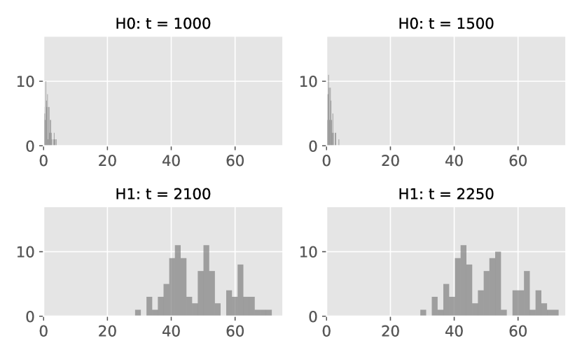
Figure 3: Histograms of $\mathrm{HC}_{t}^{\star}$ of P-values from CUSUM statistic and sparse normal mean shift, before (top) and after (bottom) the shift. The change in distribution is from $\mathcal{N}(0,1)$ to $\mathcal{N}(\mu_{r}(N),1)$, with $N=500$, $r=0.05$ and $\beta=0.5$. The change point occurs at $\tau=2000$. Each panel corresponds to a time $t$ snapshot of 100 simulated trajectories, for $t\in\{1000,1500,2100,2250\}$. The plots show that the empirical distribution of the P-values shifts after the change.

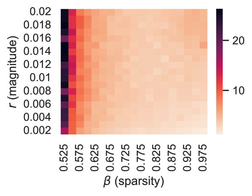
(a) EDDs/$(\rho^{\ast}(\beta,1)/r)$ regarding $(r,\beta)$

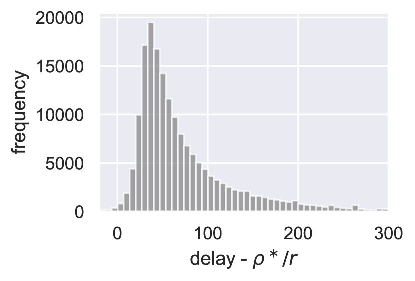
(b) Histogram of detection delay - $(\rho^{\ast}(\beta,1)/r)$ over 500 repetitions for various $(r,\beta)$

Figure 4: Simulated detection delay for a normal mean-shift from $\mathcal{N}(0,1)$ to $\mathcal{N}(\mu_{r}(N),1)$ with a fixed $\mathrm{ARL}=5000$. P-values at each sensor are computed using the exact CUSUM statistic. (a) The entries represent EDD$/(\rho^{\ast}(\beta,1)/r)$ (averaged over 500 repetitions) for various $(r,\beta)$ values. (b) Histogram for delay$-\rho^{\ast}(\beta,1)/r$ for all different $(\text{SNR},\beta)$ values from 500 repetitions.

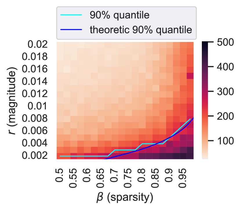
(a) EDDs regarding $(r,\beta)$

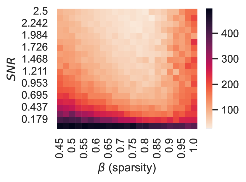
(b) EDDs regarding $({\rm SNR},\beta)$

Figure 5: Simulated detection delay for a normal mean-shift from $\mathcal{N}(0,1)$ to $\mathcal{N}(\mu_{r}(N),1)$ with a fixed $\mathrm{ARL}=5000$. P-values at each sensor are computed using the exact CUSUM statistic. (a) The entries represent EDDs (averaged over 500 repetitions) for various $(r,\beta)$ values, and we show a curve corresponding to the 90-th percentiles of the empirical EDDs. The plot shows that when the change is sparse and small, the detection delay is very large and “undetectable”; and the theoretical prediction using $\rho^{\ast}(\beta,1)/r$ givens a reasonable prediction of the observed “large EDD” detection boundary. (b) EDDs for different $(\text{SNR},\beta)$ values (over 500 repetitions), where SNR is defined as $\mu_{r}(N)^{2}\mathbb{E}[|I|\mid H_{1}]$. This plot demonstrates that for a given SNR, the EDD varies, indicating that both SNR and the sparsity of the mean shift influence detection performance.

To validate the theoretical results, we simulate a scenario where the true change occurs at $\tau=0$, and we report the empirical detection delay as a function of the change magnitude $r$ and sparsity $\beta$. The simulation is based on 500 repetitions for each combination of parameters. Figure 4 compares the simulated detection delays with the theoretical predictions. Despite differences arising from the asymptotic nature of the results, the theoretical findings are particularly helpful in identifying the “detection region”—the boundary where EDD becomes significantly larger due to sparse and weak signals. This is further illustrated in Figure 5(a), which shows the intensity map of EDDs for various $(r,\beta)$ values using the HC detection procedure. Bright areas, indicating small EDDs, correspond to cases where the change is neither too weak nor too sparse, while weaker and sparser changes lead to larger EDDs.

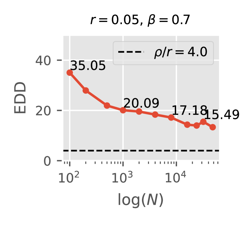
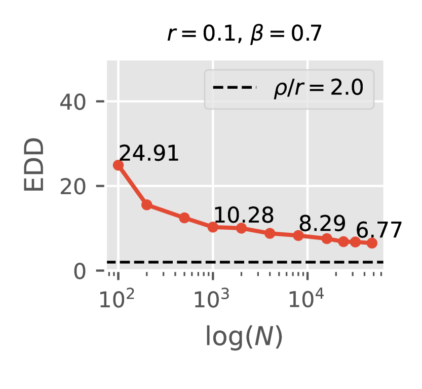
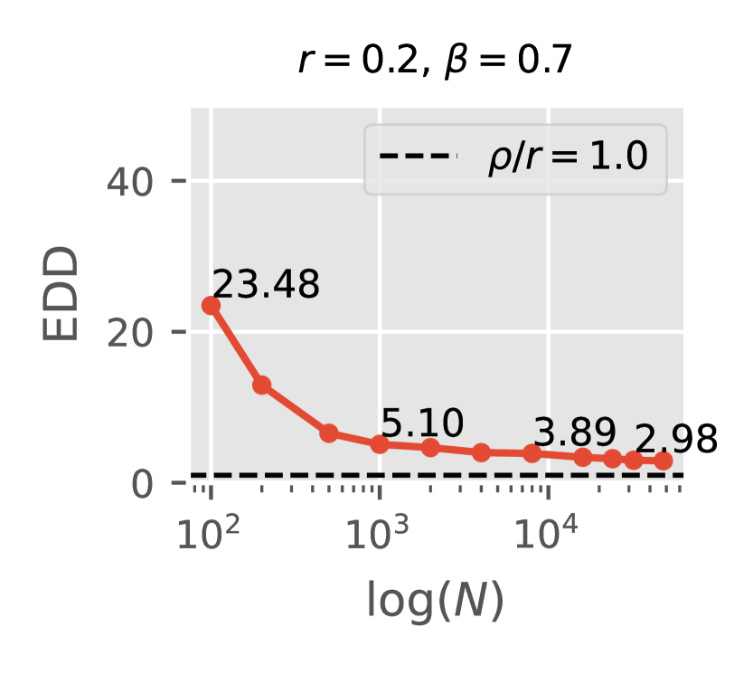
Figure 6: Convergence of the expected detection delay (EDD) to its theoretical value. Under (1) with normal mean-shift from $\mathcal{N}(0,1)$ to $\mathcal{N}(\mu_{r}(N),1)$, empirical EDDs versus $N$. ARL is fixed at $5000$. We set $\beta=0.7$ and vary $r\in\{0.05,0.1,0.2\}$. Each dashed line is the theoretical limiting detection delays $\rho^{*}(\beta,1)/r$.

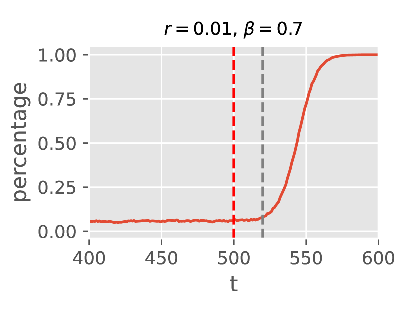
(a)

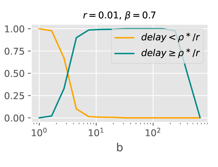
(b)

Figure 7: Observed versus asymptotic detection delay. Normal mean-shift from $\mathcal{N}(0,1)$ to $\mathcal{N}(\mu_{r}(N),1)$ with a fixed $\mathrm{ARL}=5000$, $N=20000$, where $(r,\beta)=(0.01,0.7)$. We set the time horizon $\mathcal{T}=1000$ and the change point $\tau=500$. The detection statistic at each sensor is CUSUM. We repeat the experiment 4000 times; each repetition generates one sequence of HC statistics under the same setting. (a) At each time $t$, the percentage of trajectories with detection statistic over $95\%$ quantile of detection statistic $\mathrm{HC}_{t}^{\ast}$ when there is no change (under $H_{0}$). Dashed red line corresponds to true change point $\tau$; grey dashed line corresponds to $\tau+\rho^{\ast}(\beta,1)/r$. (b) For varying threshold $b$, (orange line) the percentage of trajectories with detection delay $<\rho^{\ast}(\beta,1)/r$, versus (green line) otherwise.

Next, we analyze the phase transition of the EDD as a function of sparsity and signal-to-noise ratio (SNR). For the CUSUM procedure, the EDD is proportional to $b/{\rm KL}(f_{1}\|f_{0})$, where the Kullback-Leibler (KL) divergence in our case is given by $|I|\mu^{2}/\sigma^{2}$, representing the SNR. Figure 5(b) shows an intensity map of EDDs for different combinations of SNR and sparsity parameter $\beta$. The figure demonstrates that, despite having the same SNR, the EDD changes based on the sparsity level, indicating that classical asymptotic EDD results for the CUSUM procedure [23, 31] do not fully capture the effect of sparsity.

For a finite $N$, there is an expected gap between the empirical EDD and the theoretical detection delay $\rho^{\ast}(\beta,\sigma)/r$ due to the asymptotic nature of the result. Figure 6 illustrates this gap across different change magnitudes $r\in\{0.05,0.1,0.2\}$, showing that the gap decreases as the signal strength increases (i.e., larger $r$). Similarly, for fixed $(r,\beta)$, we observe that the gap diminishes as $N$ grows, consistent with the theoretical predictions.

To further investigate, we conducted an additional experiment with 4000 trials, analyzing the detection statistic trajectories. Figure 7(a) shows that it takes some time for the probability of raising an alarm to rise, while Figure 7(b) demonstrates that, for most threshold choices $b$, the likelihood of detecting a change when $t-\tau>\rho^{\ast}(\beta,\sigma)/r$ is significantly higher than before this time point.

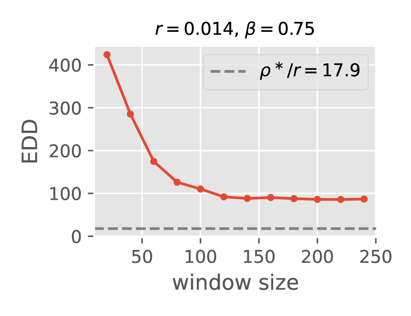
(a) $\mathrm{EDD}$ versus GLR window sizes

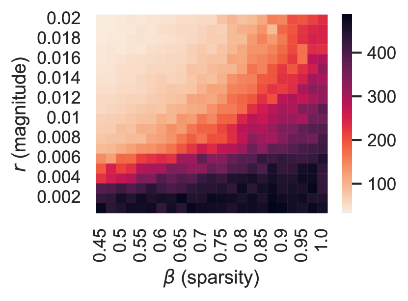
(b) $\mathrm{EDD}$ versus $(r,\beta)$

Figure 8: The problem is defined as normal mean-shift from $\mathcal{N}(0,1)$ to $\mathcal{N}(\mu_{r}(N),1)$. Each sensor using P-value computed using GLR statistic. We fixe $\mathrm{ARL}=5000$. (a) EDD versus window size for GLR statistic in (10) for $(r,\beta)=(0.014,0.75)$; the gray dashed line corresponds to theoretical prediction. (b) Phase transitions with a window size $100$. The entries are EDDs corresponding to different $(r,\beta)$.

GLR for single sensors.

We also investigate the HC procedure using P-values computed from the GLR statistics defined in (10) for the normal mean-shift problem. Figure 8(a) demonstrates that the EDD converges as the window size $w$ increases. For a fixed window size of $w=100$, Figure 8(b) illustrates that a phase transition occurs when applying WL-GLR statistics for each sensor.

5.2 Comparisons to other detection procedures

We now compare the EDDs of several procedures, each calibrated to have an approximate ARL of 5000. The corresponding thresholds are provided in Table 1. The ARLs for each procedure were estimated using Monte Carlo simulations with 500 trials. The procedures we consider are as follows, which use different strategies to combine P-values at each sensor:

1. Xie and Siegmund’s (XS) procedure [31], defined as

   $$T_{\mathrm{XS}}=\inf\left\{t:\max_{t-w\leq k<t}\sum_{n=1}^{N}\log(1-p_{0}+p_{0}e^{(W_{t,k,n}^{+})^{2}/2})>b\right\},$$

   where $W_{t,k,n}$ is formed for each sensor $n$ via (10), and the function $(z)^{+}=\max\{z,0\}$. In the experiment, we use $p_{0}=1/\sqrt{N}$, and $w=200$.

2. Chan’s procedure [7], defined as

   $$T_{\mathrm{Chan}}=\inf\left\{t:\max_{t-w\leq k<t}\sum_{n=1}^{N}g\left(W_{t,k,n}^{+}\right)\geq b\right\},$$

   where $g(z)=\log\left[1+p_{0}\left(Ce^{z^{2}/4}-1\right)\right]$ and $C=2(\sqrt{2}-1)$, and we use $p_{0}=1/\sqrt{N}$, $w=200$ in the experiments.

3. Chen and Chan’s (Chen+Chan) procedure [16]: the statistic was originally proposed for offline change-point detection, derived by examining the score statistic of P-value distribution departure from the uniform distribution. Here we modify the statistic for online change-point detection:

   $$T_{\mathrm{CC}}\left(\lambda_{1},\lambda_{2}\right)=\inf\left\{t:\sum_{n=1}^{N}\log\left(1+\frac{\lambda_{1}\log N}{N}g_{1}(\pi_{n,t})+\frac{\lambda_{2}}{\sqrt{N\log N}}g_{2}(\pi_{n,t})\right)\geq b\right\},$$

   where for $\lambda_{1}\geq 0,\,\lambda_{2}>0$, $g_{1}(z)=\frac{1}{z(2-\log z)^{2}}-\frac{1}{2}$, and $g_{2}(z)=\frac{1}{\sqrt{z}}-2$; in the experiment we choose $\lambda_{1}=1$ and $\lambda_{2}=\sqrt{\log\mathcal{T}/\log\log\mathcal{T}}$, following the same choices in [16].

4. logp sum procedure, which combines all P-values:

   $$T_{\mathrm{sum}}=\inf\left\{t:-\sum_{n=1}^{N}\log(\pi_{n,t})\geq b\right\}.$$

5. logp min procedure, which uses the “most significant” P-value:

   $$T_{\mathrm{min}}=\inf\left\{t:-\min_{n=1,\ldots,N}\log(\pi_{n,t})\geq b\right\}.$$

6. procedure based on Benjamini Hochberg (BH) statistic [4]:

   $$T_{\mathrm{BH}}=\inf\left\{t:-\min_{n=1,\ldots,N}\frac{\pi_{(n),t}}{n/N}\geq b\right\}.$$

Table 1: Thresholds $b$ for stopping rules corresponding to $\mathrm{ARL}=5000$.

	$N=100$		$N=10^{4}$
	$b$	ARL	$b$	ARL
XS [31]	19.50	4968	113.59	5000
Chan [7]	4.25	5066	4.52	5005
Chen+Chan [16]	2.89	4992	-0.66	5012
logp sum	119.60	4997	9696.15	4999
logp min	10.39	4968	14.21	5021
orderp BH	$-3.06\times 10^{-3}$	5042	$-6.77\times 10^{-3}$	5017
HC-WLCUSUM	9.93	4966	12.11	4990

Table 2: EDDs for varying $|I|$ while fixing $r=1$ and $N=100$. EDDs are calculated from 500 repetitions and the standard errors are in parentheses. In each setting, smallest EDD (up to standard errors) is bolded.

	$|I|$
	1	3	5	10	30	50	100
XS [31]	31.5 (0.56)	13.6 (0.21)	9.1 (0.13)	5.6 (0.08)	2.6 (0.03)	1.7 (0.02)	1.0 (0.01)
XS presented in [7]	31.6	14.2	10.4	6.7	3.5	2.8	2.0
Chan [7]	26.9 (0.49)	13.7 (0.21)	9.7 (0.13)	6.2 (0.08)	2.9 (0.04)	2.0 (0.02)	1.1 (0.01)
Chan presented in [7]	26.8	13.4	9.6	6.4	2.8	2.0	1.1
Chen+Chan [16]	17.7 (0.36)	11.2 (0.20)	9.3 (0.15)	6.5 (0.08)	3.5 (0.03)	2.5 (0.03)	1.8 (0.02)
logp sum	795.9 (10.66)	110.5 (4.23)	20.2 (0.25)	10.4 (0.1)	4.2 (0.04)	2.8 (0.02)	1.8 (0.02)
logp min	16.6 (0.36)	10.8 (0.20)	8.7 (0.16)	6.9 (0.11)	4.7 (0.07)	4.0 (0.06)	3.2 (0.04)
orderp BH	16.6 (0.36)	10.8 (0.20)	8.7 (0.15)	6.8 (0.11)	4.7 (0.07)	4.0 (0.06)	3.2 (0.04)
HC-WLCUSUM	16.9 (0.38)	10.6 (0.19)	8.1 (0.13)	6.0 (0.09)	3.9 (0.05)	3.1 (0.04)	2.3 (0.02)

Table 3: EDDs for varying $r$ while fixing $|I|=5$ and $N=100$. EDDs are calculated from 500 repetitions and the standard errors are in parentheses. In each setting, smallest EDD (up to standard errors) is bolded.

	$r$
	0.4	0.6	0.8	1.0	1.2	1.4
XS [31]	50.3 (0.84)	24.1 (0.36)	14.0 (0.21)	9.3 (0.13)	6.6 (0.09)	5.1 (0.07)
Chan [7]	53.1 (0.89)	25.3 (0.38)	14.9 (0.22)	9.9 (0.14)	7.0 (0.09)	5.4 (0.07)
Chen+Chan [16]	53.9 (0.86)	25.6 (0.36)	15.4 (0.22)	10.2 (0.13)	7.2 (0.09)	5.7 (0.07)
logp sum	89.8 (1.36)	45.3 (0.62)	27.3 (0.37)	18.9 (0.24)	13.9 (0.18)	11.0 (0.13)
logp min	53.4 (1.08)	24.8 (0.45)	14.4 (0.26)	9.8 (0.16)	6.9 (0.11)	5.4 (0.08)
orderp BH	53.0 (1.06)	24.6 (0.45)	14.3 (0.26)	9.6 (0.15)	6.8 (0.11)	5.3 (0.08)
HC-WLCUSUM	39.3 (0.88)	18.8 (0.38)	10.9 (0.21)	7.5 (0.13)	5.3 (0.09)	4.2 (0.07)

Table 4: EDDs for varying $|I|$, while fixing $r=1$ and $N=10^{4}$. EDDs are calculated from 500 repetitions, and the standard errors are in parentheses. In each setting, the smallest EDD (up to standard errors) is bolded. “–” denotes “failure to detect”: the procedure did not raise an alarm by the end of the detection time horizon 1000 for all sequences. “N/A” means that a specific result is not available.

	$|I|$
	$1$	$5$	$10$	$10^{2}$	$10^{3}$	$10^{4}$
XS [31]	64.5 (0.9)	20.8 (0.22)	13.9 (0.12)	4.0 (0.03)	1.0 (0.0)	1.0 (0.0)
Chan [7]	37.3 (0.54)	18.0 (0.2)	13.3 (0.13)	4.5 (0.04)	1.0 (0.0)	1.0 (0.0)
Chan presented in [7]	37.7	N/A	13.3	4.5	1.0	1.0
Chen+Chan [16]	870.9 (5.67)	35.2 (0.31)	23.5 (0.16)	9.6 (0.05)	3.7 (0.02)	1.0 (0.0)
logp sum	–	999.9 (0.07)	998.1 (0.59)	263.4 (0.79)	7.2 (0.02)	1.0 (0.0)
logp max	25.8 (0.47)	15.5 (0.24)	12.7 (0.18)	7.2 (0.09)	4.2 (0.05)	2.8 (0.03)
orderp BH	25.8 (0.47)	15.5 (0.24)	12.6 (0.18)	7.1 (0.09)	4.2 (0.05)	2.7 (0.03)
HC-WLCUSUM	25.8 (0.47)	15.3 (0.23)	12.4 (0.17)	6.7 (0.08)	3.5 (0.03)	1.0 (0.0)

Table 5: EDDs for varying $r$, while fixing $|I|=10$, and $N=10^{4}$. EDDs are calculated from 500 repetitions, and the standard errors are in parentheses. In each setting, the smallest EDD (up to standard errors) is bolded.

	$r$
	$0.4$	$0.6$	$0.8$	$1.0$	$1.2$	$1.4$
XS [31]	79.7 (0.88)	36.7 (0.4)	21.2 (0.21)	13.8 (0.13)	9.9 (0.09)	7.4 (0.07)
Chan [7]	76.9 (0.92)	35.3 (0.41)	20.5 (0.21)	13.4 (0.13)	9.4 (0.09)	7.1 (0.07)
Chen+Chan [16]	135.2 (1.05)	61.5 (0.49)	36.0 (0.28)	23.5 (0.17)	16.8 (0.11)	12.7 (0.09)
logp sum	997.9 (0.54)	997.2 (0.73)	997.4 (0.83)	997.6 (0.66)	997.9 (0.68)	997.4 (0.62)
logp max	70.7 (1.23)	32.4 (0.55)	19.3 (0.29)	12.6 (0.19)	9.0 (0.13)	6.9 (0.09)
orderp BH	70.5 (1.22)	32.3 (0.55)	19.3 (0.29)	12.6 (0.19)	9.0 (0.13)	6.8 (0.09)
HC-WLCUSUM	69.7 (1.19)	31.8 (0.53)	18.9 (0.28)	12.3 (0.18)	8.8 (0.12)	6.7 (0.09)

To ensure a fair comparison, we tune the thresholds $b$ for each procedure to achieve the same target ARL of 5000. The thresholds, determined through trial and error over 500 repetitions, are listed in Table 1. We evaluate the methods under the following settings for moderate and high dimensions: (i) $N=100$, $r=1$, with varying $|I|$; (ii) $N=100$, $|I|=5$, with varying $r$; (iii) $N=10^{4}$, $r=1$, with varying $|I|$; and (iv) $N=10^{4}$, $|I|=10$, with varying $r$.

For a moderate scale problem with $N=100$, the EDD results are presented in Tables 2 (varying $|I|$ with fixed $r$) and 3 (varying $r$ with fixed $|I|$). In setting (i), the HC-based procedure achieves the smallest EDDs for relatively sparse shifts ($|I|=1,3,5$), while the XS procedure performs best in denser cases. In setting (ii), where the sparsity is fixed at $|I|=5$ and the shift magnitude $r$ varies, the HC-based procedure consistently outperforms other methods across different values of $r$ for sparse shifts.

For larger-scale experiments with $N=10^{4}$, the EDD results are shown in Tables 4 and 5. The HC-based procedure achieves the smallest EDDs for relatively sparse shifts ($|I|=1,5,10$). In Table 5, with fixed sparsity $|I|=10$ and varying $r$, the HC-based procedure consistently performs well. As a sanity check, Tables 2 and 4 also include results for the XS and Chan methods from [7], which closely match our reproduced results.

6 Discussion

In this paper, we introduced a new change-point detection procedure that combines P-values from individual sensors using higher criticism (HC). We analyzed the asymptotic detection delay of this procedure under a sparse heteroscedastic normal change point. Our numerical experiments validate the theoretical detection delay characterization and further demonstrate the superior performance of our HC-based procedure compared to other detection procedures.

Several limitations to our work invite further exploration. We did not fully characterize the information-theoretic detection delay, as alternative tests applied to individual sensors might perform better. For instance, the likelihood ratio (LR) test assumes a known post-change mean but not the post-change variance. Additionally, our analysis is asymptotic in the number of sensors $N$, but is limited to a finite time horizon $\mathcal{T}$. This results in a coarser characterization of the EDD compared to studies such as [7] and [16], which consider an arbitrary time horizon and an ARL lower bound of $\gamma\sim e^{N^{\zeta}}$, with $\zeta\in(0,1)$. Despite this, our experiments show that HC performs well compared to other tests under arbitrarily large ARL requirements.

For future work, it would be valuable to extend the analysis approach to other sparse data models. For example, the work of [19] suggests that the most interesting tradeoff between change intensity and sparsity occurs when changes follow a moderate deviation scale in $N$. This insight suggests that sparse sequential change-point detection based on HC has optimality properties under a variety of data models with affected sensors experiencing a moderate change in the distribution. It is also interesting to explore sparse sequential change-point detection under non-moderate distribution changes such as those studied in [2, 18, 3, 1, 13] for sparse (offline) anomaly detection.

7 Proof

We now present the proof of the main result. In Section 7.1, we provide the necessary background on offline hypothesis testing for rare and weak moderately departure models, as well as the asymptotic behavior of log-chi-squared P-values. Section 7.2 shows that the P-values relevant to this paper satisfy these properties. Section 7.3 proves the main result.

7.1 Background

Rare (sparse) and weak models for signal detection involve detection or classification challenges in which most of the features are useless (pure noise), except perhaps very few features. The locations of the useful features, if there are any, are unknown to us in advance [9, 17, 18]. As explained in [19], previously studied rare and weak models in which departures of non-null features are on the moderate deviation scale can be carried out under the following testing problem, involving independent P-values $\{\pi_{n}\}_{n=1}^{N}$ from individual features.

$$\begin{split}H_{0}\,&:\,\pi_{n}\sim\mathrm{Unif}(0,1),\quad\forall n=1,\ldots,N,\\ H_{1}^{(N)}\,&:\,\pi_{n}\sim(1-p)\mathrm{Unif}(0,1)+pQ_{n}^{(N)},\quad\forall n=1,\ldots,N,\end{split}$$ (15)

where the sequence of distributions $\{Q_{n}^{(N)}\}_{n=1}^{N}$ obey:

$$X_{n}\overset{\mathsf{iid}}{\sim}Q_{n}^{(N)}\Leftrightarrow\lim_{N\to\infty}\max_{n=1,\ldots,N}\left|\frac{-\log\Pr\left[-2\log X_{n}\geq 2q\log(N)\right]}{\log(N)}-\left(\frac{\sqrt{q}-\sqrt{\rho}}{\sigma}\right)^{2}\right|=0,$$ (16)

for all $q>\rho>0$. A sufficient condition for the validity of (16) is that

$$-2\log Q_{n}^{(N)}\overset{D}{=}\left(\sqrt{2\rho\log(N)}+\sigma Z\right)^{2}(1+o_{p}(1)),\quad Z\sim\mathcal{N}(0,1),$$

where $o_{p}(1)$ indicates a sequence tending to zero in probability as $N\to\infty$ uniformly in $n$. Indeed, if $q>\rho$, for $N$ large enough

$$\Pr\left[\left(\sqrt{2\rho\log(N)}+\sigma Z\right)^{2}(1+o_{p}(1))\geq 2q\log(N)\right] =2\Pr\left[\frac{(\sqrt{2q}-\sqrt{2\rho})\sqrt{\log(N)}}{\sigma}(1+o(1))\leq Z\right]$$

$$=N^{-\left(\frac{\sqrt{q}-\sqrt{\rho}}{\sigma}\right)^{2}+o(1)},$$

the last transition by Mill’s ratio [26].

The name “asymptotically log-chisquared” is because (16) holds in particular when

$$X_{n}\overset{D}{=}\exp\left\{-\frac{1}{2}\left(\sqrt{2\rho\log(N)}+\sigma Z\right)^{2}\right\}.$$

Namely, when the $X_{n}$’s follow a non-central log-chisquared distribution over one degree of freedom. As explained in [19], models involving moderate departures in individual features falling under the formulation (16) share many common properties concerning the asymptotic behavior of testing procedures. One important property in our case is the asymptotic power of a test based on the higher criticism of the P-values.

Also, for ranked P-values, $\pi_{(1)}\leq\pi_{(2)}\leq\cdots\leq\pi_{(N)}$, and $\mathrm{HC}^{\star}$ defined in (5), we have

Theorem 2.

[19, Thms. 1 & 2] Fix $\rho>0$, $\sigma>0$, and $\beta>0$. Assume that $p=N^{-\beta}$ and that $\{\pi_{n}\}_{n=1}^{N}$ follow (15). If $\rho>\rho^{*}(\beta,\sigma)$, there exists a sequence $\{b_{N}\}$ such that

$$\lim_{N\to\infty}\left(\Pr\left[\mathrm{HC}^{\star}<b_{N}|H_{1}\right]+\Pr\left[\mathrm{HC}^{\star}\geq b_{N}|H_{0}\right]\right)\to 0.$$

If $\rho<\rho^{*}(\beta,\sigma)$, for any sequence of thresholds $\{b_{N}\}$,

$$\liminf_{N\to\infty}\left(\Pr\left[\mathrm{HC}^{\star}<b_{N}|H_{1}\right]+\Pr\left[\mathrm{HC}^{\star}\geq b_{N}|H_{0}\right]\right)=1.$$

7.2 Log-chisquared properties of P-values of change-point detection statistics

We provide conditions under which the P-values of the likelihood ratio and generalized likelihood ratio are asymptotically log-chisquared. These conditions coincide with the asymptotic calibration of the intensity of individual change points and their sparsity to $N$ in [7, 16]. One notable difference is the lower bound on the ARL $\gamma$, which we assume to go to infinity but at a rate arbitrarily small. This is a weaker result than the rate of $\log(\gamma)N^{-\zeta}\to 0$ provided in [7].

Recall that for the CUSUM and GLR procedures, monitoring for a change in the data’s distribution based on $Y_{t}^{\mathsf{LR}}$ or $Y_{t}^{\mathsf{GLR}}$ involves the stopping times

$$T_{x}^{\mathsf{LR}}:=\inf\{t\,:\,Y_{t}^{\mathsf{LR}}\geq x\},$$

and

$$T_{x}^{\mathsf{GLR}}:=\inf\{t\,:\,Y_{t}^{\mathsf{GLR}}\geq x\}.$$

Recall that the P-values $\pi_{t}^{\mathsf{LR}}(x)$ and $\pi_{t}^{\mathsf{GLR}}(x)$ the survival functions of the statistics $Y_{t}^{\mathsf{LR}}$ and $Y_{t}^{\mathsf{GLR}}$ under the null. If we plug in the corresponding observed statistics value to replace $x$, we get P-values under the model (15).

7.2.1 Properties of tests under the null

The distribution of $Y_{t}^{\square}$, $\square\in\{\mathsf{LR},\mathsf{GLR}\}$ is continuous under either $H_{0}$ or $H_{1}$. Therefore, under $H_{0}$, we have

$$\pi_{t}^{\square}(Y_{t}^{\square})\sim\mathrm{Unif}(0,1),\qquad t=1,\ldots,\mathcal{T}.$$ (17)

In practice, we obtain the distribution of $Y_{t}^{\square}$ by Monte Carlo simulations involving multiple draws of an individual sequence $\{X_{t}\}$. On the other hand, a considerable effort in the literature on change point detection focused on characterizing the “steady state” null behavior of $Y_{t}^{\square}$. The following two lemmas use such results to provide the asymptotic behavior of $\pi_{t}^{\square}$, from which we can obtain asymptotic P-values as an alternative to simulations.

Lemma 1.

Consider $\pi_{t}^{\mathsf{LR}}$ of (9). As $x\to\infty$ and $\log(t)/x\to 0$,

$$-2\log\pi_{t}^{\mathsf{LR}}(x)=2x(1+o(1))$$ (18)

uniformly in $t$.

Theorem 3 (Theorem 1 in [27]).

As $x\rightarrow\infty$, under $H_{0}$, $T_{x}^{\mathsf{GLR}}$ is asymptotically exponentially distributed with expectation

$$\mathbb{E}\left[T_{x}^{\mathsf{GLR}}\right]\sim\frac{(2\pi)^{1/2}\exp(x^{2}/2)}{x\int_{0}^{\infty}z\nu^{2}(z)dz},$$ (19)

where the special function

$$\nu(x)=\frac{2}{x^{2}}\exp\left\{-2\sum_{n=1}^{\infty}\frac{1}{n}\Phi\left(-\frac{x\sqrt{n}}{2}\right)\right\},$$

with $\Phi$ the standard normal cumulative distribution function.

Lemma 2.

Suppose that $x\to\infty$ and $t\to\infty$ such that $t\leq cx^{2}$ for some $c>0$. Then under $H_{0}$,

$$-2\log\pi_{t}^{\mathsf{GLR}}(x)=x^{2}(1+o(1)),$$ (20)

where $o(1)\to 0$.

Remark 1.

The asymptotic expressions in Lemmas 1 and 2 are valid when $t\to\infty$. Our analysis is therefore restricted to this case.

Regardless, we may always use instead the statistics:

$$\tilde{\pi}_{t}^{\mathsf{LR}}(Y_{t}^{\mathsf{LR}}) =e^{-Y_{t}^{\mathsf{LR}}},$$

$$\tilde{\pi}_{t}^{\mathsf{GLR}}(Y_{t}^{\mathsf{GLR}}) =e^{-(Y_{t}^{\mathsf{GLR}})^{2}/2},$$

which are asymptotic P-values under the null and satisfy the expressions in Lemmas 1 and 2. The results on the asymptotic power of HC from [19] apply to these asymptotic P-values.

7.2.2 Properties of tests under a change in distribution

The following lemma shows that the maximum in $Y_{t}^{\mathsf{GLR}}$ and $Y_{t}^{\mathsf{LR}}$ are attained after the change with probability approaching one provided $t$ does not grow faster than the increase in the mean shift. This property seems well-known for $Y_{t}^{\mathsf{LR}}$ based on the discussion in [27]. In our situation, the proof appears simpler than in previous cases because we let the individual effect size $\mu_{N}\to\infty$. This lemma justifies the analysis of the P-values assuming $\tau=1$ (change at time $0$) and may also simplify the analysis of the behavior of $\pi_{t}^{\mathsf{GLR}}(x)$ under $H_{1}$.

Lemma 3.

Consider $V_{t,k}$ of (8) and $W_{t,k}$ of (10). Suppose that $X_{1},\ldots,X_{\tau-1}\overset{\mathsf{iid}}{\sim}\mathcal{N}(0,1)$ and $X_{\tau},\ldots,X_{\mathcal{T}}\overset{\mathsf{iid}}{\sim}\mathcal{N}(\mu_{N},\sigma^{2})$ for some $1\leq\tau\leq\mathcal{T}$, $\sigma^{2}>0$, and $\mu_{N}$ such that $\mu_{N}\to\infty$ and $\mu_{N}/\sqrt{\log(\mathcal{T})}\to\infty$ as $N,\mathcal{T}\to\infty$. Then, uniformly in $t,\tau\leq\mathcal{T}$,

$$\lim_{N\to\infty}\Pr\left[\arg\max_{k\leq t}V_{t,k}<\tau\right]=0$$

and

$$\lim_{N\to\infty}\Pr\left[\arg\max_{k\leq t}W_{t,k}<\tau\right]=0.$$

Lemma 4.

Consider $V_{t,k}$ of (8). Suppose that $X_{1},\ldots,X_{\tau-1}\overset{\mathsf{iid}}{\sim}\mathcal{N}(0,1)$ and $X_{\tau},\ldots,X_{\mathcal{T}}\overset{\mathsf{iid}}{\sim}\mathcal{N}(\mu_{N},\sigma^{2})$ for some $1\leq\tau\leq\mathcal{T}$, $\sigma^{2}>0$, and $\mu_{N}\to\infty$. Then, uniformly in $\tau,t\leq\mathcal{T}$,

$$\lim_{N\to\infty}\Pr\left[Y_{t}^{\mathsf{LR}}=\max_{\tau\leq k\leq t}V_{t,k}\right]=1.$$

The following claim says that with probability going to $1$, the maximum in the LR statistic is attained at the change point $k=\tau$.

Lemma 5.

Assume that $\mu\to\infty$, and for $\tau\geq 1$ we have $X_{1},\ldots,X_{\tau-1}\overset{\mathsf{iid}}{\sim}\mathcal{N}(0,1)$ and $X_{\tau},\ldots,X_{\mathcal{T}}\overset{\mathsf{iid}}{\sim}\mathcal{N}(\mu,\sigma^{2})$. Then

$$\lim_{N\to\infty}\Pr\left[Y_{t}^{\mathsf{LR}}=V_{t,\tau}\right]=1,$$

uniformly in $\tau,t\leq\mathcal{T}$.

Lemma 6.

Consider $W_{t,k}$ of (10). Suppose that $X_{1},\ldots,X_{\tau-1}\overset{\mathsf{iid}}{\sim}\mathcal{N}(0,1)$ and $X_{\tau},\ldots,X_{\mathcal{T}}\overset{\mathsf{iid}}{\sim}\mathcal{N}(\mu,\sigma^{2})$ for some $1\leq\tau\leq\mathcal{T}$, $\sigma^{2}>0$, and $\mu\to\infty$. Then

$$\lim_{N\to\infty}\Pr\left[Y_{t}^{\mathsf{GLR}}=\max_{\tau\leq k\leq t}W_{t,k}\right]=1,$$

uniformly in $\tau,t\leq\mathcal{T}$.

Lemma 7.

Consider $W_{t,k}$ of (10). Suppose that $X_{\tau},\ldots,X_{\mathcal{T}}\overset{\mathsf{iid}}{\sim}\mathcal{N}(\mu_{N},\sigma^{2})$ for some $1\leq\tau\leq\mathcal{T}$, $\sigma^{2}>0$, and $\mu_{N}\to\infty$. For $\tau\leq v\leq t$

$$\Pr\left[W_{t,\tau}\leq W_{t,v}\right]\leq\exp\left\{-\frac{1}{2}\frac{\mu^{2}(v-\tau)}{5\sigma^{2}}\right\}(1+o(1)),$$ (21)

with $o(1)$ independent of $t$ and $\tau$.

The following claim says that with probability going to $1$, the maximum in the GLR statistic is attained at the change point $k=\tau$.

Lemma 8.

Assume that $\mu\to\infty$. If $X_{1},\ldots,X_{\tau-1}\overset{\mathsf{iid}}{\sim}\mathcal{N}(0,1)$ and $X_{\tau},\ldots,X_{\mathcal{T}}\overset{\mathsf{iid}}{\sim}\mathcal{N}(\mu,\sigma^{2})$.

$$\lim_{N\to\infty}\Pr\left[Y_{t}^{\mathsf{GLR}}=W_{t,\tau}\right]=1,$$

uniformly in $t$ and $\tau$.

Lemma 9.

Assume that $\mu_{N}(r)=\sqrt{2r\log(N)}$ for some $r>0$, and for some $\tau\geq 1$ we have $X_{1},\ldots,X_{\tau-1}\overset{\mathsf{iid}}{\sim}\mathcal{N}(0,1)$ and $X_{\tau},\ldots,X_{\mathcal{T}}\overset{\mathsf{iid}}{\sim}\mathcal{N}(\mu_{N}(r),\sigma^{2})$. Set $\Delta:=t-\tau+1$. For any $t>\tau$,

$$-2\log\pi_{t}^{\mathsf{LR}}(Y_{t}^{\mathsf{LR}})=\left(\sigma Z+\mu_{N}(r\Delta)\right)^{2}(1+o_{p}(1)),$$ (22)

where $o_{p}(1)$ represents a RV that goes to $0$ in probability as $N\to\infty$, uniformly in $t$ and $\tau$.

Lemma 10.

Assume that $\mu_{N}(r)=\sqrt{2r\log(N)}$ for some $r>0$, and for some $\tau\geq 1$ we have $X_{1},\ldots,X_{\tau-1}\overset{\mathsf{iid}}{\sim}\mathcal{N}(0,1)$ and $X_{\tau},\ldots,X_{\mathcal{T}}\overset{\mathsf{iid}}{\sim}\mathcal{N}(\mu_{N}(r),\sigma^{2})$. Set $\Delta:=t-\tau+1$. For any $t>\tau$,

$$-2\log\pi_{t}^{\mathsf{GLR}}(Y_{t}^{\mathsf{GLR}})\overset{D}{=}\left(\mu_{N}(r\Delta)+\sigma Z\right)^{2}(1+o_{p}(1))$$

7.3 Proof of main result

Now we will put everything together to prove the main result for the detection delay in multi-sensor with sparse, moderately large change points. Now let $I\subset\{1,\ldots,N\}$ be a random set of indices such that $\Pr\left[n\in I\right]=p$ with different indices independent of each other. Recall that the data obeys

$$X_{n,t}\sim\begin{cases}\mathcal{N}(0,1),&n\neq I\quad\text{or }t=1\ldots,\tau-1\\ \mathcal{N}(\mu,\sigma^{2}),&t=\tau,\ldots,\mathcal{T},\end{cases}$$ (23)

where the paths $\{X_{n,t}\}_{t\geq 1}$ are independent for different $n=1,\ldots,N$. Consider a global change-point model:

$$H_{0}^{(N)}: \tau>\mathcal{T},$$ (24)

$$H_{1}^{(N)}: \tau\leq\mathcal{T}.$$

We note that $\tau>\mathcal{T}$ indicates no change.

Before stating our main result, we provide a more general result concerning the detection delay in rare moderate departures setup using higher criticism.

Theorem 4.

Let $I$ be a random set such that $\Pr\left[n\in I\right]=p$ independently for all $n=1,\ldots,N$. Suppose that

$$\pi_{n,t}\sim\begin{cases}\mathrm{Unif}(0,1),&n\neq I\text{ or }t=1,\ldots,\tau-1,\\ Q_{nt}^{(N)},&t=\tau,\ldots,\mathcal{T},\end{cases}$$ (25)

where every $Q_{nt}^{(N)}$ obeys (16) with $\rho=\rho_{t}$. Let $\Delta(\beta,\sigma)$ denote the minimal $t$ such that $\rho_{t}>\rho^{*}(\beta,\sigma)$ and $\infty$ otherwise. As $N\to\infty$, for fixed $\mathcal{T}>0$ arbitrarily large, and a stopping time $T_{\mathrm{HC}}=\inf\{t:\mathrm{HC}_{t}^{\star}>b_{t}^{(N)}\},$ there exists an array of thresholds $\{b_{t}^{(N)},\,t=1,\ldots,\mathcal{T};\,N=1,2,\ldots\}$ such that,

$$\Pr\left[T_{\mathrm{HC}}=\Delta(\beta,\sigma)|H_{1}^{(N)}\right]\to 1$$

while

$$\Pr\left[T_{\mathrm{HC}}\leq\mathcal{T}|H_{0}^{(N)}\right]\to 0.$$

Remark 2.

• We added here a restriction that $\mathcal{T}$ is fixed in $N$. The reason is that we do not know how fast $\Pr\left[\mathrm{HC}_{t}^{\star}\geq b_{t}^{(N)}\mid H_{0}\right]\to 0$. Presumably, we can choose $b_{t}^{(N)}$ so that $\max_{t}\Pr\left[\mathrm{HC}_{t}^{\star}\geq b_{t}^{(N)}\right]\sim e^{-cN}$, in which case $\mathcal{T}\sim e^{(c-\delta)N}$ for some small $\delta$. However, the current analysis of HC from [9] and [19] do not explicitly offer this kind of result. This means that our lower bound on the ARL is $\mathcal{T}$ and must be fixed (to an arbitrarily large value). We should through simulations that this technical restriction does not appear to limit the practicality of the detection scheme.

• Even if we can have

  $$\max_{t}\Pr\left[\mathrm{HC}_{t}^{\star}\geq b_{t}^{(N)}\right]\sim e^{-cN},$$

  our lower bound on the ARL is $\mathcal{T}\sim N^{\zeta}$ for $\zeta\to 0$ due to the Lemma 3. This is more restrictive than the case $ARL\sim N^{\zeta}$ for arbitrary $\zeta$ considered in [7].

• Theorem 1 shows in particular that $\mathrm{EDD}=\mathbb{E}\left[D|H_{1}\right]\to\rho^{*}(\beta,\sigma)/r$, hence $\mathrm{HC}_{t}^{\star}$ attains the information-theoretic lower bound of [7] when $\zeta=0$ and $\sigma=1$.

• The heteroscedastic component ($\sigma^{2}$ after the change) is not included in [7]. Based on the discussion in [19] and [6], an increase in variance assists in detecting a change. The worst situation for detection is when the series changes to a constant ($\sigma=0$).

• In the setting of [7], the mean shift is $r$ compared to $\sqrt{2r\log(N)}$ in our case. As a result, we tie the detection delay directly to $\rho^{*}(\beta,\sigma)$. Our calibration is more informative and in agreement with the literature on rare and weak signal detection.

• We can also prove a theorem of the form: The detection delay of any stopping rule that is based on (10) is at most $\rho^{*}(\beta,\sigma)/r$.

Proof of Theorem 1.

Let $t^{*}$ be the minimal $t$ such that $\rho_{t}=r(t-\tau+1)$ exceeds $\rho^{*}(\beta,\sigma)$. We have

$$t^{*}-\tau+1=\lceil\rho^{*}(\beta,\sigma)/r\rceil.$$

In view of Theorem 4, it is enough to show that $\pi_{nt}^{\square}$ are of the form (25) with $\rho_{t}=r(t-\tau+1)$. For this purpose, it is enough to show that for an affected series $n\in I$, $\pi_{n,t}^{\square}$ obey (16) with $\rho=r(t-\tau+1)$. When $\square=\mathsf{LR}$, this follows from Lemma 1. When $\square=\mathsf{GLR}$, this follows Lemma 2. ∎

Appendix A Proof details

Proof of Lemma 1.

A standard result in change-point detection says that as $x\to\infty$ and $t\to\infty$ with $\log(t)/x\to 0$,

$$e^{x}\Pr\left[Y_{t}^{\mathsf{LR}}\geq x\right]/t\to C$$

for some constant $C$. (c.f. [32, Ch 4.3]). Consequently,

$$-2\log\pi_{t}^{\mathsf{LR}}(x) =-2\log\Pr\left[Y_{t}^{\mathsf{LR}}\geq x\right]$$

$$=2x-2\log(Ct)+o(1)$$

$$=2x(1-\log(C)/x-\log(t)/x)+o(1)$$

$$=2x(1+o(1))$$

∎

Proof of Lemma 2.

It follows from Theorem 3 that under $H_{0}$ and $t/x^{2}=O(1)$, $T_{x}$ is asymptotically exponentially distributed with mean

$$\mu_{x}:=\mathbb{E}\left[T_{x}|H_{0}\right]=\sqrt{2\pi}\frac{e^{x^{2}/2}}{xC},$$

where $C$ is some numerical constant. Therefore, for $x>0$ we may write

$$\Pr\left[Y_{t}^{\mathsf{GLR}}\geq x\right] =\Pr\left[T_{x}\leq t\right]$$

$$=(1-e^{-t/\mu_{x}})(1+o(1))=t/\mu_{x}(1+o(1)).$$

It follows that

$$-2\log\Pr\left[Y_{t}^{\mathsf{GLR}}\geq x\right] =2\log(\mu_{x})-2\log(t)+o(1)$$

$$=x^{2}+2\log\frac{\sqrt{2\pi}}{xC}-2\log(t)+o(1)$$

$$=x^{2}(1+o(1)).$$

∎

Proof of Lemma 3.

Consider the following events defined by $X_{1},\ldots,X_{\mathcal{T}}$.

$$\Omega_{V_{t}} :=\{\arg\max_{k\leq t}V_{t,k}<\tau\},$$

$$\Omega_{W_{t}} :=\{\arg\max_{k\leq t}W_{t,k}<\tau\},$$

$$B_{t} :=\left\{\text{$\exists$ $0<m<\tau$, $0\leq k\leq t-\tau$, such that $X_{\tau-m}\geq X_{\tau+k}$ }\right\}.$$

Note that

$$\Omega_{V_{t}}\subset B_{t}\text{ and }\Omega_{W_{t}}\subset B_{t}.$$

Consequently, it is enough to show that $\Pr\left[B_{t}\right]\to 0$.

Let $Z_{1},\ldots,Z_{m}\overset{\mathsf{iid}}{\sim}\mathcal{N}(\mu,\sigma^{2})$. Then

$$\Pr\left[\min\{Z_{1},\ldots,Z_{m}\}\leq a\right] =1-\left(1-\Phi\left(\frac{a-\mu}{\sigma}\right)\right)^{m}=1-\Phi^{m}\left(\frac{\mu-a}{\sigma}\right).$$

$$\Pr\left[\max\{Z_{1},\ldots,Z_{m}\}\leq a\right] =\Phi^{m}\left(\frac{a-\mu}{\sigma}\right).$$

Define $A_{a}=\{\max\{X_{1},\ldots X_{\tau-1}\}\leq a\}$. We have

$$\Pr\left[B_{t}\right] =\Pr\left[\max\{X_{1},\ldots,X_{\tau-1}\}\geq\min\{X_{\tau},\ldots,X_{\mathcal{T}}\}\right]$$

$$\leq\Pr\left[\max\{X_{1},\ldots,X_{\tau-1}\}\geq\min\{X_{\tau},\ldots,X_{\mathcal{T}}\}|A_{a}\right]\Pr\left[A_{a}\right]+\Pr\left[A_{a}^{c}\right]$$

$$\leq\Pr\left[a\geq\min\{X_{\tau},\ldots,X_{\mathcal{T}}\}|A_{a}\right]+\Pr\left[A_{a}^{c}\right]$$

$$=1-\Phi^{\mathcal{T}-\tau+1}\left(\frac{\mu_{N}-a}{\sigma}\right)+\Pr\left[A_{a}^{c}\right].$$

Let $a=\sqrt{4\log\mathcal{T}}$, then recall that $\Phi(x)\sim 1-\phi(x)/x$

$$\Pr\left[A_{a}\right]=\Phi^{\tau-1}(\sqrt{4\log\mathcal{T}})\geq\Phi^{\mathcal{T}}(\sqrt{4\log\mathcal{T}})\sim\left(1-\frac{e^{-2\log\mathcal{T}}}{\sqrt{8\pi\log\mathcal{T}}}\right)^{\mathcal{T}}=1+o(1),$$

hence $\Pr\left[A_{a}^{c}\right]\to 0$ as $N\to\infty$. Additionally, since $\mu_{N}\to\infty$ and $\mu_{N}/\sqrt{\log(\mathcal{T})}\to\infty$, also $\mu_{N}-\sqrt{4\log(\mathcal{T})}\to\infty$ and we can use the upper bound $1-\Phi(x)\leq e^{-x^{2}/2}/\sqrt{2\pi}$ as $x\to\infty$. This implies that for all $N$ large enough,

$$\Phi^{\mathcal{T}-\tau}\left(\frac{\mu_{N}-\sqrt{4\log\mathcal{T}}}{\sigma}\right) \geq\Phi^{\mathcal{T}}\left(\frac{\mu_{N}-\sqrt{4\log\mathcal{T}}}{\sigma}\right)$$

$$\sim\left(1-e^{-\frac{1}{2}\left(\mu_{N}-\sqrt{4\log(\mathcal{T})}\right)^{2}}\right)^{\mathcal{T}}$$

$$=\left(1-e^{-2\log(\mathcal{T})\left(\frac{\mu_{N}}{\sqrt{4\log(\mathcal{T})}}-1\right)^{2}}\right)^{\mathcal{T}}$$

$$\geq\left(1-e^{-2\log(\mathcal{T})}\right)^{\mathcal{T}}=1+o(1),$$

where the last transition is because $\mu_{N}/\sqrt{\log(\mathcal{T})}\to\infty$. We conclude that $\Pr\left[B_{t}\right]=o(1)$ which completes the proof of the lemma. ∎

Proof of Lemma 4.

Recall that $V_{t,m}=\mu\left[\sum_{j=m+1}^{t}X_{j}-\frac{\mu}{2}(t-m)\right]$, which is distributed as $\mathcal{N}(\frac{\mu^{2}}{2}(t-m),\mu^{2}(t-m))$ under $H_{1}$. For $\tau\leq m\leq t$,

$$\Pr\left[V_{t,m}<0\right] =\Pr\left[\mathcal{N}\left(\mu^{2}(t-m)/2,\mu^{2}(t-m)\right)<0\right]$$

$$=\Phi\left(-\mu\sqrt{t-m}/2\right)=e^{-\mu^{2}(t-m)/8}(1+o(1)).$$ (26)

In addition,

$$\max_{k\leq m}V_{m,k}-\max_{k\leq t}V_{t,k} \leq\max_{k\leq m}(V_{m,k}-V_{t,k})=-V_{t,m}.$$

Therefore,

$$\Pr\left[\max_{k\leq m}V_{m,k}-\max_{k\leq t}V_{t,k}>0\right]\leq\Pr\left[-V_{t,m}>0\right]=e^{-\mu^{2}(t-m)/8}(1+o(1)).$$

where the last equality is due to (26). Consider the event

$$B_{u,t}:=\{\exists\,u\leq m<t\,:\,\max_{k\leq m}V_{m,k}>\max_{k\leq t}V_{t,k}\}.$$

Notice that

$$\Pr\left[Y_{t}^{\mathsf{LR}}>\max_{\tau\leq k\leq t}V_{t,k}\right]\leq\Pr\left[B_{1,t}\right]\leq\Pr\left[B_{1,\tau}\right]+\Pr\left[B_{\tau,t}\right].$$

The first inequality is because the event

$$\{Y_{t}^{\mathsf{LR}}>\max_{\tau\leq k\leq t}V_{t,k}\}=\{\max_{1\leq k\leq t}V_{t,k}>\max_{\tau\leq k\leq t}V_{t,k}\}=\{\max_{1\leq k\leq\tau}V_{t,k}>\max_{\tau\leq k\leq t}V_{t,k}\}=\{\max_{1\leq k\leq\tau}V_{t,k}\geq\max_{1\leq k\leq t}V_{t,k}\},$$

and the last event by definition is $B_{1,t}$.

By similar arguments as in Lemma 3, $\Pr\left[B_{1,\tau}\right]=o(1)$. Additionally,

$$\Pr\left[B_{\tau,t}\right] \leq o(1)+\sum_{m=\tau}^{t-1}\Pr\left[\max_{k\leq m}V_{m,k}-\max_{k\leq t}V_{t,k}>0\right]$$

$$\leq(1+o(1))\sum_{m=\tau}^{t-1}e^{-\mu^{2}(t-m)/8}$$

$$\leq(1+o(1))\frac{e^{-\mu^{2}/8}}{1-e^{-\mu^{2}/8}}=o(1).$$

By definition, we have that $Y_{t}^{\mathsf{LR}}\geq\max_{\tau\leq k\leq t}V_{t,k}$. We conclude

$$\Pr\left[Y_{t}^{\mathsf{LR}}\neq\max_{\tau\leq k\leq t}V_{t,k}\right]=\Pr\left[Y_{t}^{\mathsf{LR}}>\max_{\tau\leq k\leq t}V_{t,k}\right]=o(1).$$

This completes the proof. ∎

Proof of Lemma 5.

By Lemma 4, we may assume

$$Y_{t}^{\mathsf{LR}}=\max_{\tau\leq k\leq t}V_{t,k},$$

almost surely, since the probability of the complementary event vanishes as $N\to\infty$. Since $Y_{t}^{\mathsf{LR}}\geq V_{t,\tau}$, it is enough to show that $\Pr\left[Y_{t}^{\mathsf{LR}}\geq V_{t,k}+\epsilon\right]\to 0$ for any $\epsilon>0$. Let $\mu:=\mu_{N}(r)>0$. In the following, $Z_{1},\ldots Z_{m}$ is a sequence of independent standard normal random variables. $\sum_{i=1}^{0}Z_{i}\equiv 0$. Fix $\epsilon>0$.

$$\Pr\left[Y_{t}^{\mathsf{LR}}\geq V_{t,\tau}+\epsilon\right] =\Pr\left[\max_{\tau\leq k\leq t}\left\{{S_{t}-S_{k}-\frac{\mu}{2}(t-k)}\right\}\geq S_{t}-S_{\tau}-\frac{\mu}{2}(t-\tau)+\frac{\epsilon}{\mu}\right]$$

$$=\Pr\left[\max_{\tau\leq k\leq t}{\left\{{\color[rgb]{0,0,0}S_{\tau}-S_{k}-\frac{\mu}{2}(\tau-k)}\right\}}\geq\frac{\epsilon}{\mu}\right]$$

$$=\Pr\left[\max_{\tau\leq k\leq t}\left\{-\left(S_{k}-S_{\tau}-\frac{\mu}{2}(k-\tau)\right)\right\}\geq\frac{\epsilon}{\mu}\right]$$

$$=\Pr\left[\max_{\tau\leq k\leq t}\left\{-\left(S_{k}-S_{\tau}-\mu(k-\tau)\right)-\frac{\mu}{2}(k-\tau)\right\}\geq\frac{\epsilon}{\mu}\right]$$

$$=\Pr\left[\min_{0\leq m\leq t-\tau}\left\{\sigma\sum_{i=1}^{m}Z_{i}+\frac{\mu}{2}m\right\}\leq-\frac{\epsilon}{\mu}\right]$$

$$=\Pr\left[\left\{\sigma Z_{1}+\frac{\mu}{2}\leq-\frac{\epsilon}{\mu}\right\}\cup\left\{\sigma(Z_{1}+Z_{2})+2\frac{\mu}{2}\leq-\frac{\epsilon}{\mu}\right\}\cup\right.\cdots$$

$$\qquad\qquad\left.\cup\left\{\sigma\sum_{i=1}^{t-\tau}Z_{i}+(t-\tau)\frac{\mu}{2}\leq-\frac{\epsilon}{\mu}\right\}\right]$$

$$\leq\sum_{m=1}^{t-\tau}\Pr\left[\sigma\sum_{i=1}^{m}Z_{i}+m\frac{\mu}{2}\leq-\frac{\epsilon}{\mu}\right]=\sum_{m=1}^{t-\tau}\Pr\left[\sigma\sqrt{m}Z_{1}+m\frac{\mu}{2}\leq-\frac{\epsilon}{\mu}\right]$$

$$=\sum_{m=1}^{t-\tau}\Phi\left(\frac{-\frac{\epsilon}{\mu}-m\mu/2}{\sigma\sqrt{m}}\right)\leq\sum_{m=1}^{t-\tau}\Phi\left(-\frac{\sqrt{m}\mu}{2\sigma}\right)$$

$$\leq\frac{1}{\sigma\sqrt{2\pi}}\sum_{m=1}^{t-\tau}e^{-m\mu^{2}/(8\sigma^{2})}\leq\frac{1}{\sigma\sqrt{2\pi}}\frac{e^{-\mu^{2}/(8\sigma^{2})}}{1-e^{-\mu^{2}/(8\sigma^{2})}}.$$

The proof is completed by noticing that, as $\mu\to\infty$, the last expression converges to zero and is independent of $t$. ∎

Proof of Lemma 6.

The proof is similar to the proof of Lemma 4. Simply replace (26) with Lemma 7 below. ∎

Proof of Lemma 7.

In the following, for integers$\tau<v<t$, denote $S_{t,v}:=S_{t}-S_{v}$. We have

$$\Pr\left[W_{t,\tau}<W_{t,v}\right] =\Pr\left[\frac{S^{2}_{t,\tau}}{t-\tau}<\frac{S^{2}_{t,v}}{t-v}\right]$$

$$=\Pr\left[\frac{S^{2}_{t,v}}{t-\tau}+\frac{S^{2}_{v,\tau}}{t-\tau}+2\frac{S_{t,v}S_{v,\tau}}{t-\tau}<\frac{S^{2}_{t,v}}{t-v}\right]$$

$$=\Pr\left[S^{2}_{t,v}\frac{v-\tau}{t-v}>S^{2}_{v,\tau}+2S_{t,v}S_{v,\tau}\right]$$

where the second equality uses the fact that $S_{t,\tau}=S_{t,v}+S_{v,\tau}$ and the third equality follows by grouping terms with $S_{t,v}^{2}$. We now solve the quadratic equation for $S_{t,v}$. This leads to

$$\Pr\left[W_{t,\tau}<W_{t,v}\right] \leq\Pr\left[S_{t,v}\frac{v-\tau}{t-v}>S_{v,\tau}\left(1+\sqrt{1+\frac{v-\tau}{t-v}}\right)\right]$$

$$\qquad+\Pr\left[S_{t,v}\frac{v-\tau}{t-v}<S_{v,\tau}\left(1-\sqrt{1+\frac{v-\tau}{t-v}}\right)\right].$$

The second term goes to zero as $N$ goes to infinity whenever $v>\tau$ because the probability that one of $S_{t,v}$ and $S_{v,\tau}$ is negative goes to zero as their mean increases to infinity. We proceed by handling the first term. We denote by $Z_{1}$, $Z_{2}$, and $Z_{3}$ three independent standard normal RVs. Using that $S_{v,\tau}$ is independent of $S_{t,v}$ and both are sums of several independent $\mathcal{N}(\mu,\sigma^{2})$, we get

$$\Pr\left[S_{t,v}\frac{v-\tau}{t-v}>S_{v,\tau}\left(1+\sqrt{1+\frac{v-\tau}{t-v}}\right)\right]$$

$$=\Pr\left[\frac{S_{t,v}}{t-v}>\frac{S_{v,\tau}}{v-\tau}\left(1+\sqrt{1+\frac{v-\tau}{t-v}}\right)\right]$$

$$=\Pr\left[\frac{\sigma Z_{1}}{\sqrt{t-v}}+\mu>(\frac{\sigma Z_{2}}{\sqrt{v-\tau}}+\mu)\left(1+\sqrt{1+\frac{v-\tau}{t-v}}\right)\right]$$

$$=\Pr\left[\frac{Z_{1}}{\sqrt{t-v}}>\frac{Z_{2}}{\sqrt{v-\tau}}\left(1+\sqrt{1+\frac{v-\tau}{t-v}}\right)+\frac{\mu}{\sigma}\sqrt{1+\frac{v-\tau}{t-v}}\right]$$

$$=\Pr\left[Z_{1}\sqrt{v-\tau}>Z_{2}\left(\sqrt{t-v}+\sqrt{t-\tau}\right)+\frac{\mu}{\sigma}\sqrt{t-\tau}\sqrt{v-\tau}\right]$$

$$=\Pr\left[Z_{3}\geq\frac{\mu}{\sigma}\sqrt{\frac{(t-\tau)(v-\tau)}{v-\tau+\left(\sqrt{t-v}+\sqrt{t-\tau}\right)^{2}}}\right]$$

$$\leq\Pr\left[Z_{3}\geq\frac{\mu}{\sigma}\sqrt{\frac{(t-\tau)(v-\tau)}{t-\tau+\left(\sqrt{t-\tau}+\sqrt{t-\tau}\right)^{2}}}\right]$$

$$=\Pr\left[Z_{3}\geq\frac{\mu}{\sigma}\sqrt{\frac{v-\tau}{5}}\right]=1-\Phi\left(\frac{\mu\sqrt{v-\tau}}{\sqrt{5}\sigma}\right).$$

From here, the advertised claim follows by Mill’s ratio. ∎

Proof of Lemma 8.

By Lemma 6, we may assume

$$Y_{t}^{\mathsf{GLR}}=\max_{\tau\leq k\leq t}W_{t,k},$$

since the probability of the complementary event vanishes as $N\to\infty$. For $\tau<v\leq t$, we use Lemma 7 and the union bound to conclude

$$\Pr\left[\exists v>\tau\,:\,W_{t,\tau}<W_{t,v}\right]\leq\Pr\left[\{W_{t,\tau}<W_{t,\tau+1}\}\cup\cdots\{W_{t,\tau}<W_{t,t-1}\}\right]$$

$$\leq\sum_{v=\tau+1}^{t-1}\Pr\left[W_{t,\tau}<W_{t,v}\right]\leq\frac{1}{\sqrt{10\pi\sigma^{2}}}\sum_{v=\tau+1}^{t-1}e^{-\frac{\mu^{2}(v-\tau)}{5\sigma^{2}}}$$

$$\leq\frac{1}{\sqrt{10\pi\sigma^{2}}}\frac{e^{-\frac{\mu^{2}}{5\sigma^{2}}}}{1-e^{-\frac{\mu^{2}/2}{5\sigma^{2}}}}\to 0,$$

uniformly in $t$ as as $n\to\infty$. ∎

Proof of Lemma 9.

Note that

$$V_{t,\tau} \overset{D}{=}\left(\sqrt{\Delta}\sigma Z+\frac{\Delta}{2}\mu_{N}(r)\right)\mu_{N}(r)=\frac{1}{2}\left(\sigma Z+\sqrt{\Delta}\mu_{N}(r)\right)^{2}-\sigma^{2}Z^{2}/2$$

$$=\frac{1}{2}\left(\sigma Z+\mu_{N}(r\Delta)\right)^{2}-\sigma^{2}Z^{2}/2$$

$$=\frac{1}{2}\left(\sigma Z+\mu_{N}(r\Delta)\right)^{2}(1+o_{p}(1)),$$

where in the last transition we used that $\mu_{N}(r)\to\infty$ as $N\to\infty$ and that

$$\frac{Z^{2}}{\mu_{N}^{2}(r(\Delta))}\sim N^{-r\Delta}\to 0.$$

In particular, $V_{t,\tau}$ is unbounded in $N$. By Lemma 8,

$$Y_{t}^{\mathsf{LR}}=V_{t,\tau}+o_{p}(1),$$

From the above and using Lemma 1,

$$-2\log\pi_{t}^{\mathsf{LR}}(Y_{t}^{\mathsf{LR}}) =-2Y_{t}^{\mathsf{LR}}(1+o_{p}(1))$$

$$=-2(V_{t,\tau}+o_{p}(1))(1+o_{p}(1))=-2(V_{t,\tau})(1+o_{p}(1))$$

$$=\left(\sigma Z+\mu_{N}(r\Delta)\right)^{2}(1+o_{p}(1)).$$

∎

Proof of Lemma 10.

Note that

$$W_{t,\tau}^{2}\overset{D}{=}\left(\sqrt{\Delta}\mu_{N}(r)+\sigma Z\right)^{2}=\left(\mu_{N}(r\Delta)+\sigma Z\right)^{2},\qquad Z\sim\mathcal{N}(0,1).$$

By Lemma 8,

$$(Y_{t}^{\mathsf{GLR}})^{2}=W_{t,\tau}^{2}+o_{p}(1)\overset{D}{=}\left(\mu_{N}(r\Delta)+\sigma Z\right)^{2}+o_{p}(1),$$

where $o_{p}(1)$ represents a RV that goes to $0$ in probability as $N\to\infty$, uniformly in $t$. From here, Lemma 2, and continuous mapping,

$$-2\log\pi_{t}^{\mathsf{GLR}}(Y_{t}^{\mathsf{GLR}}) \overset{D}{=}(Y_{t}^{\mathsf{GLR}})^{2}(1+o_{p}(1))$$

$$\overset{D}{=}\left(\mu_{N}(r\Delta)+\sigma Z\right)^{2}(1+o_{p}(1)).$$

In the last transition, we used $\mu_{N}(r)\to\infty$ as $n\to\infty$. ∎

Proof of Theorem 4.

For every fixed $t=1,\ldots,\mathcal{T}$, the P-values $\pi_{1t},\ldots,\pi_{Nt}$ obey (15) with

$$\rho=\begin{cases}0&t=1,\ldots,\tau-1,\\ \rho_{t}&t=\tau,\ldots,\mathcal{T}.\end{cases}$$

Set $\rho^{*}:=\rho^{*}(\beta,\sigma)$. Theorem 2 implies that if $\rho_{t}>\rho^{*}$, there exists a sequence of thresholds $b_{t}^{(N)}$ such that

$$\Pr\left[\mathrm{HC}_{t}^{\star}<b_{t}^{(N)}\mid H_{1}^{(N)}\right]\to 0,$$

while

$$\Pr\left[\mathrm{HC}_{t}^{\star}\geq b_{t}^{(N)}\mid H_{0}^{(N)}\right]\to 0,$$

Thus, for fixed $\mathcal{T},$ we have

$$\mathcal{T}\max_{t\,:\,\rho_{t}<\rho^{*}}\Pr\left[\mathrm{HC}_{t}^{\star}\geq b_{t}^{(N)}\mid H_{1}^{(N)}\right]\to 0,$$

and

$$\mathcal{T}\max_{t}\Pr\left[\mathrm{HC}_{t}^{\star}\geq b_{t}^{(N)}\mid H_{0}^{(N)}\right]\to 0.$$

It follows that

$$\Pr\left[T_{\mathrm{HC}}\leq\mathcal{T}\mid H_{0}^{(N)}\right] =\Pr\left[\cup_{t\leq\mathcal{T}}\{\mathrm{HC}_{t}^{\star}\geq b_{t}^{(N)}\}\mid H_{0}^{(N)}\right]$$

$$\leq\mathcal{T}\max_{t}\Pr\left[\mathrm{HC}_{t}^{\star}\geq b_{t}^{(N)}\mid H_{0}^{(N)}\right]\to 0.$$ (27)

Similarly, if $\Delta(\beta,\sigma)=\infty$, then $\rho_{t}<\rho^{*}$ and

$$\Pr\left[T_{\mathrm{HC}}\leq\mathcal{T}\mid H_{1}^{(N)}\right] =\Pr\left[\cup_{t\leq\mathcal{T}}\{\mathrm{HC}_{t}^{\star}\geq b_{t}^{(N)}\}\mid H_{1}^{(N)}\right]$$

$$\leq\mathcal{T}\max_{t}\Pr\left[\mathrm{HC}_{t}^{\star}\geq b_{t}^{(N)}\mid H_{1}^{(N)}\right]\to 0.$$ (28)

If $\Delta(\beta,\sigma)<\infty$, then

$$\Pr\left[T_{\mathrm{HC}}>\Delta(\beta,\sigma)\mid H_{1}^{(n)}\right]\leq 1-\Pr\left[\mathrm{HC}_{\Delta(\beta,\sigma)}\geq b_{t}^{(N)}\right]\to 0,$$ (29)

and

$$\Pr\left[T_{\mathrm{HC}}<\Delta(\beta,\sigma)\mid H_{1}^{(n)}\right] \leq\Pr\left[\cup_{t\,:\,\rho_{t}<\rho^{*}}\{\mathrm{HC}_{t}^{\star}\geq b_{t}^{(N)}\}\right]$$

$$\leq\mathcal{T}\max_{t\,:\,\rho_{t}<\rho^{*}}\Pr\left[\mathrm{HC}_{t}^{\star}\geq b_{t}^{(N)}\right]\to 0.$$ (30)

Since the events in (29) and (30) are disjoint,

$$\Pr\left[T_{\mathrm{HC}}=\Delta(\beta,\sigma)|H_{1}^{(N)}\right]\to 1.$$

The proof is completed given the last convergence and (27). ∎

References

- [1] Ery Arias-Castro, Rong Huang, and Nicolas Verzelen. Detection of sparse positive dependence. Electronic Journal of Statistics, 14(1):702 – 730, 2020.
- [2] Ery Arias-Castro and Meng Wang. The sparse Poisson means model. Electronic Journal of Statistics, 9(2):2170–2201, 2015.
- [3] Ery Arias-Castro and Andrew Ying. Detection of sparse mixtures: Higher criticism and scan statistic. Electronic Journal of Statistics, 13(1):208–230, 2019.
- [4] Yoav Benjamini and Yosef Hochberg. Controlling the false discovery rate: A practical and powerful approach to multiple testing. Journal of the Royal Statistical Society: Series B (Methodological), 57(1):289–300, 1995.
- [5] Shankar Bhamidi, Jimmy Jin, and Andrew Nobel. Change point detection in network models: Preferential attachment and long range dependence. The Annals of Applied Probability, 28(1):35–78, 2018.
- [6] T. Tony Cai, X. Jessie Jeng, and Jiashun Jin. Optimal detection of heterogeneous and heteroscedastic mixtures. Journal of the Royal Statistical Society: Series B (Statistical Methodology), 73(5):629–662, 2011.
- [7] Hock Peng Chan. Optimal sequential detection in multi-stream data. The Annals of Statistics, 45(6):2736–2763, 2017.
- [8] Hock Peng Chan and Guenther Walther. Optimal detection of multi-sample aligned sparse signals. The Annals of Statistics, 43(5):1865 – 1895, 2015.
- [9] David Donoho and Jiashun Jin. Higher criticism for detecting sparse heterogeneous mixtures. The Annals of Statistics, 32(3):962–994, 2004.
- [10] David Donoho and Jiashun Jin. Higher criticism thresholding: Optimal feature selection when useful features are rare and weak. Proceedings of the National Academy of Sciences, 105(39):14790–14795, 2008.
- [11] David Donoho and Jiashun Jin. Feature selection by higher criticism thresholding achieves the optimal phase diagram. Philosophical Transactions of the Royal Society A: Mathematical, Physical and Engineering Sciences, 367(1906):4449–4470, 2009.
- [12] David Donoho and Jiashun Jin. Higher criticism for large-scale inference, especially for rare and weak effects. Statistical Science, 30(1):1 – 25, 2015.
- [13] David L Donoho and Alon Kipnis. Higher criticism to compare two large frequency tables, with sensitivity to possible rare and weak differences. The Annals of Statistics, 50(3):1447–1472, 2022.
- [14] Farida Enikeeva and Zaid Harchaoui. High-dimensional change-point detection under sparse alternatives. The Annals of Statistics, 47(4):2051 – 2079, 2019.
- [15] Josua Gösmann, Christina Stoehr, Johannes Heiny, and Holger Dette. Sequential change point detection in high dimensional time series. Electronic Journal of Statistics, 16(1):3608–3671, 2022.
- [16] Shouri Hu, Jingyan Huang, Hao Chen, and Hock Peng Chan. Likelihood scores for sparse signal and change-point detection. IEEE Transactions on Information Theory, 69(6):4065–4080, 2023.
- [17] Jiashun Jin. Impossibility of successful classification when useful features are rare and weak. Proceedings of the National Academy of Sciences, 106(22):8859–8864, 2009.
- [18] Jiashun Jin and Zheng Tracy Ke. Rare and weak effects in large-scale inference: Methods and phase diagrams. Statistica Sinica, pages 1–34, 2016.
- [19] Alon Kipnis. Unification of rare/weak detection models using moderate deviations analysis and log-chisquared p-values. Statistica Scinica, 2023. to appear.
- [20] Tze Leung Lai. Information bounds and quick detection of parameter changes in stochastic systems. IEEE Transactions on Information Theory, 44(7):2917–2929, 1998.
- [21] Erich L Lehmann and Joseph P Romano. Testing Statistical Hypotheses. Springer Science & Business Media, 2006.
- [22] Shuang Li, Yao Xie, Hanjun Dai, and Le Song. Scan b-statistic for kernel change-point detection. Sequential Analysis, 38(4):503–544, 2019.
- [23] G Lorden. Procedures for reacting to a change in distribution. The Annals of Mathematical Statistics, 42(6):1897–1908, 1971.
- [24] Emmanuel Pilliat, Alexandra Carpentier, and Nicolas Verzelen. Optimal multiple change-point detection for high-dimensional data. Electronic Journal of Statistics, 17(1):1240–1315, 2023.
- [25] Moshe Pollak. Optimal detection of a change in distribution. The Annals of Statistics, 13(1):206–227, 1985.
- [26] Galen R Shorack and Jon A Wellner. Empirical processes with applications to statistics. SIAM, 2009.
- [27] David Siegmund and ES Venkatraman. Using the generalized likelihood ratio statistic for sequential detection of a change-point. The Annals of Statistics, pages 255–271, 1995.
- [28] Ivo V Stoepker, Rui M Castro, Ery Arias-Castro, and Edwin van den Heuvel. Anomaly detection for a large number of streams: A permutation-based higher criticism approach. Journal of the American Statistical Association, 119(545):461–474, 2024.
- [29] Alexander G Tartakovsky and Venugopal V Veeravalli. General asymptotic bayesian theory of quickest change detection. Theory of Probability & Its Applications, 49(3):458–497, 2005.
- [30] Liyan Xie, Shaofeng Zou, Yao Xie, and Venugopal V Veeravalli. Sequential (quickest) change detection: Classical results and new directions. IEEE Journal on Selected Areas in Information Theory, 2(2):494–514, 2021.
- [31] Yao Xie and David Siegmund. Sequential multi-sensor change-point detection. The Annals of Statistics, 41(2):670 – 692, 2013.
- [32] Benjamin Yakir. Extremes in random fields: A theory and its applications. John Wiley & Sons, 2013.
Acknowledgement
This work is partially supported by an NSF CAREER CCF-1650913, NSF DMS-2134037, CMMI-2015787, CMMI-2112533, DMS-1938106, DMS-1830210, ONR N000142412278, and the Coca-Cola Foundation.