Detecting Change Points of Covariance Matrices
in High Dimensions

Abstract

Testing for change points in sequences of high-dimensional covariance matrices is an important and equally challenging problem in statistical methodology with applications in various fields. Motivated by the observation that even in cases where the ratio between dimension and sample size is as small as $0.05$, tests based on a fixed-dimension asymptotics do not keep their preassigned level, we propose to derive critical values of test statistics using an asymptotic regime where the dimension diverges at the same rate as the sample size.

This paper introduces a novel and well-founded statistical methodology for detecting change points in a sequence of high-dimensional covariance matrices. Our approach utilizes a min-type statistic based on a sequential process of likelihood ratio statistics. This is used to construct a test for the hypothesis of the existence of a change point with a corresponding estimator for its location. We provide theoretical guarantees for these inference tools by thoroughly analyzing the asymptotic properties of the sequential process of likelihood ratio statistics in the case where the dimension and sample size converge with the same rate to infinity. In particular, we prove weak convergence towards a Gaussian process under the null hypothesis of no change. To identify the challenging dependency structure between consecutive test statistics, we employ tools from random matrix theory and stochastic processes. Moreover, we show that the new test attains power under a class of alternatives reflecting changes in the bulk of the spectrum, and we prove consistency of the estimator for the change-point location.

, and

1 Introduction

Having its origins in quality control (see Wald, 1945; Page, 1954, for two early references), change point detection has been an extremely active field of research until today with numerous applications in finance, genetics, seismology or sports to name just a few. In the last decade, a large part of the literature on change point detection considers the problem of detecting a change point in a high-dimensional sequence of means (see Jirak, 2015; Cho and Fryzlewicz, 2015; Dette and Gösmann, 2020; Enikeeva and Harchaoui, 2019; Liu et al., 2020; Liu, Gao and Samworth, 2021; Chen, Wang and Wu, 2022; Wang et al., 2022; Zhang, Wang and Shao, 2022, among many others).

Compared to the huge amount of work on the change-point problem for a sequence of high-dimensional means, the literature on the problem of detecting structural breaks in the corresponding covariance matrices is more scarce. For the low dimensional setting we refer to Chen and Gupta (2004), Lavielle and Teyssiere (2006), Galeano and Peña (2007), Aue et al. (2009) and Dette and Wied (2016), among others, who study different methods and aspects of the change point problem under the assumption that the sample size converges to infinity while the dimension is fixed. We also refer to Theorem 1.1.2 in Csörgő and Horváth (1997) who provide a test statistic and its asymptotic distribution under the null hypothesis for normal distributed data. However, even in cases where the ratio between dimension and sample size is rather small, it can be observed that statistical guarantees derived from fixed-dimension asymptotics can me be misleading. Exemplary, we display in Table 1 the simulated type I error of two commonly used tests for a change point in the in a sequence of covariance matrices. The first method (CH) is based on sequential likelihood ratio statistics, where the critical values have been determined by classical asymptotic arguments assuming that the dimension is fixed (see Theorem 1.1.2 in Csörgő and Horváth, 1997). The second approach (AHHR) is a test proposed by Aue et al. (2009), which is based on a quadratic form of the vectorized CUSUM statistic of the empirical covariance matrix. Again, the determination of critical values relies on fixed-dimensional asymptotics. We observe that even in the case where the ratio between the dimension and sample size is as small as $0.05$, the nominal level $\alpha=0.05$ of the CH test is exceeded by more than a factor of three. On the other hand, the AHHR test provides only a reasonable approximation of the nominal level, if the ratio between dimension and sample size is $0.025$. Note that this test requires the inversion of an estimate of high-dimensional covariance matrix and is only applicable if the sample size is larger than the squared dimension.

Dimension		5	10	15	20	25
Empirical level	CH	0.05	0.16	0.39	0.82	1.00
	AHHR	0.03	0.01	0.00	-	-

Table 1: Simulated type I errors of the sequential likelihood ratio test (Theorem 1.1.2 in Csörgő and Horváth, 1997) and the test of Aue et al. (2009) ($500$ simulation runs, nominal level $\alpha=0.05$, standard normally distributed data). Critical values are determined by fixed dimension asymptotics for a sample size of $n=200$. If ”-” is reported, the corresponding test is not applicable.

Meanwhile, several authors have also discussed the problem of estimating a change point in a sequence of covariance matrices in the high-dimensional regime. For example, Avanesov and Buzun (2018) propose a multiscale approach to estimate multiple change points, while Wang, Yu and Rinaldo (2021) investigate the optimality of binary and wild binary segmentation for multiple change point detection. We also mention the work of Dette, Pan and Yang (2022), who propose a two-stage approach to detect the location of a change point in a sequence of very high-dimensional covariance matrices. Li and Gao (2024) pursue a similar approach to develop a change-point test for high-dimensional correlation matrices.

With respect to testing, the literature on change point detection is rather scarce. In principle, one can develop change point analysis based on a vectorization of the covariance matrices using inference tools for a sequence of means. This approach essentially boils down to comparing the matrices before and after the change point with respect to a vector norm. However, in general, this approach does not yield an asymptotically distribution free test statistic. Moreover, as pointed out by Ryan and Killick (2023), such distances do not reflect the geometry induced on the space of positive definite matrices. These authors propose a change-point test based on an alternative distance defined on the space of positive definite matrices, which compares sequentially the multivariate ratio $\mathbf{\Sigma}^{-1}_{1}\mathbf{\Sigma}_{2}$ of the two covariance matrices $\mathbf{\Sigma}_{1}$ and $\mathbf{\Sigma}_{2}$ before and after a potential change point with the identity matrix. As a consequence, under the null hypothesis of no change point, their test statistic is independent of the underlying covariance structure, which makes it possible to derive quantiles for statistical testing in the regime where the dimension diverges at the same rate as the sample size. However, the approach of these authors is based on a combination of a point-wise limit theorem from random matrix theory with a Bonferroni correction. Therefore, as pointed out in Section 4 of Ryan and Killick (2023), the resulting test may be conservative in applications. Moreover, this methodology is tailored to centered data, and it is demonstrated in Zheng, Bai and Yao (2015), that an empirical centering introduces a non-negligible bias in the central limit theorem for the corresponding linear spectral statistic.

In this paper, we propose an alternative test for detecting a change point in a sequence of high-dimension covariance matrices, which takes the strong dependence between consecutive test statistics into account to avoid the drawbacks of previous works. Our approach is based on a sequential process of likelihood ratio test (LRT) statistics, where the dimension of the data is growing with the dimension at the same rate. We combine tools from random matrix theory and stochastic processes to develop and analyze statistical methodology for change point analysis in the covariance structure of high-dimensional data. Random matrix theory is a common tool to investigate asymptotic properties of LRT in high-dimensional scenarios for classical testing problems. An early reference in this direction is Jiang and Yang (2013), who establish central limit theorems for several classical LRT statistics under the null hypotheses. Since this seminal work, numerous researchers have investigated related problems (see Jiang and Qi, 2015; Dette and Dörnemann, 2020; Bao et al., 2022; Dörnemann, 2023; Heiny and Parolya, 2023; Parolya, Heiny and Kurowicka, 2024, among others). None of these papers considers sequential LRT statistics to develop change point analysis. Moreover, these references do not contain any consistency results. In general, the body of literature concerning LRTs under alternative hypotheses in the high-dimensional regime remains sparse; for some exceptions, see Chen and Jiang (2018), Bodnar, Dette and Parolya (2019) and Bai and Zhang (2023). Having this line of literature in mind, we can summarize the main contributions of this paper.

1. Enhancing the power of the min-type statistic. We propose a novel methodology to test for a change point in a sequence of high-dimensional covariance matrices based on a minimum of sequential LRT statistics. Under the null hypothesis, this statistic admits a simple limiting distribution in the regime where the dimension diverges proportionally to the sample size. Unlike most other approaches, the new test does not require the estimation of the population covariance matrix. This result facilities the introduction of a simple asymptotic testing procedure with favorable finite-sample properties. Most notably, our approach takes the strong dependency structure between consecutive test statistics into account, whose analysis has been recognized as a challenging problem in the literature (see Ryan and Killick, 2023), and which has not been addressed in previous works.

2. Power analysis and change-point estimation. We also study asymptotic properties of the sequential process under alternative hypotheses to identify conditions which guarantee the consistency of the test. The techniques developed in this paper are believed to be a valuable contribution to study consistency for other problems as well.

   Besides developing a testing methodology with desirable properties, we also introduce a new estimator of the change-point location based on the LRT principle. Our comprehensive analysis of the process of LRT statistics enables us to provide theoretical guarantees under which the estimator admits consistency.

3. Mathematical challenges. Investigating sequential statistics introduces new challenges in random matrix theory compared to consideration of the common (non-sequential) LRT, namely (i) the convergence of the finite-dimensional distributions and (ii) the asymptotic tightness of the sequential log-LRT statistics. Indeed, the weak convergence result implied by (i) and (ii) is a novel, technically challenging contribution, given that sequential LRT statistics have not been studied in such a functional and high-dimensional framework before.

   To establish (i), we derive an asymptotic representation of the test statistics and apply a martingale CLT to the dominating term in this decomposition. Note that for given time points $t_{1},t_{2}\in[0,1]$, the corresponding LRT statistics are highly correlated, and a nuanced analysis is required in order to determine their covariance. Regarding (ii), we show asymptotic equicontinuity of the sequential log-LRT statistics by deriving uniform inequalities for the moments of the corresponding increments.

The remaining part of this work is structured as follows. In Section 2, we present the new method to detect and estimate a change-point in a high-dimensional covariance structure, and provide the main theoretical guarantees. In numerical experiments given in Section 3, we compare the finite-sample size properties of our test as well as the change-point estimator to other approaches. The proofs of our theoretical results are deferred to Section 4 and the supplementary material.

2 Change point analysis by a sequential LRT process

Let $\mathbf{y}_{1},\ldots,\mathbf{y}_{n}$ be a sample of independent random vectors such that $\mathbf{y}_{i}=(y_{1i},\ldots,y_{pi})^{\top}=\mathbf{\Sigma}_{i}^{1/2}\mathbf{x}_{i}$ for i.i.d. $p$-dimensional random vectors $\mathbf{x}_{i}$ and covariance matrices $\mathbf{\Sigma}_{i}=\mathbf{\Sigma}_{i,n}$, $1\leq i\leq n.$ We are interested in testing for a change in the covariance structure of $\mathbf{y}_{1},\ldots,\mathbf{y}_{n}$, and consider the hypotheses

$$H_{0}: \mathbf{\Sigma}_{1}=\ldots=\mathbf{\Sigma}_{n}$$ (2.1)

versus

$$H_{1}: \mathbf{\Sigma}_{1}=\ldots=\mathbf{\Sigma}_{\lfloor nt^{\star}\rfloor}\neq\mathbf{\Sigma}_{\lfloor nt^{\star}\rfloor+1}=\ldots=\mathbf{\Sigma}_{n},$$ (2.2)

where the location $t^{\star}\in(t_{0},1-t_{0})$ of the change point is unknown and $t_{0}>0$ is a positive constant. We define

$$\hat{\mathbf{\Sigma}}_{i:j}^{\textnormal{cen}} =\frac{1}{j-i}\sum\limits_{k=i}^{j}\left(\mathbf{y}_{j}-\overline{\mathbf{y}}_{i:j}\right)\left(\mathbf{y}_{j}-\overline{\mathbf{y}}_{i:j}\right)^{\top},\quad 1\leq i\leq j\leq n,$$ (2.3)

as the sample covariance matrices calculated from the data $\mathbf{y}_{i},\ldots,\mathbf{y}_{j}$, where

$$\overline{\mathbf{y}}_{i:j}=\frac{1}{j-i+1}\sum_{k=i}^{j}\mathbf{y}_{i}$$

denotes the sample mean of $\mathbf{y}_{i},\ldots,\mathbf{y}_{j}$. Finally, we define

$$\hat{\mathbf{\Sigma}}^{\textnormal{cen}} =\hat{\mathbf{\Sigma}}_{1:n}^{\textnormal{cen}},$$ (2.4)

as the sample covariance matrix calculated from the full sample and consider the statistic

$$\Lambda_{n,t}^{\textnormal{cen}}=\frac{\big{|}\hat{\mathbf{\Sigma}}^{\textnormal{cen}}_{1:\lfloor nt\rfloor}\big{|}^{\frac{1}{2}\lfloor nt\rfloor}\big{|}\hat{\mathbf{\Sigma}}^{\textnormal{cen}}_{(\lfloor nt\rfloor+1):n}\big{|}^{\frac{1}{2}(n-\lfloor nt\rfloor)}}{\big{|}\hat{\mathbf{\Sigma}}^{\textnormal{cen}}\big{|}^{\frac{1}{2}n}},\quad t\in(0,1).$$ (2.5)

If, for fixed $t$, $\mathbf{y}_{1},\ldots,\mathbf{y}_{\lfloor nt\rfloor}$ and $\mathbf{y}_{\lfloor nt\rfloor+1},\ldots,\mathbf{y}_{n}$ are two independent samples of i.i.d. random variables with $\mathbb{E}[\mathbf{y}_{1}]=\mu_{1}$, Var$(\mathbf{y}_{1})=\mathbf{\Sigma}_{1}$ and $\mathbb{E}[\mathbf{y}_{n}]=\mu_{n}$, Var$(\mathbf{y}_{n})=\mathbf{\Sigma}_{n}$, then $\Lambda_{n,t}^{\textnormal{cen}}$ is the likelihood ratio test statistic (LRT) for the hypotheses $\tilde{H}_{0}:~{}\mathbf{\Sigma}_{1}=\mathbf{\Sigma}_{n},~{}\mu_{1}=\mu_{n}$ versus $\tilde{H}_{1}:~{}\mathbf{\Sigma}_{1}\neq\mathbf{\Sigma}_{n}$. This problem has been investigated by several authors in the high-dimensional regime (see, for example, Li and Chen, 2012; Jiang and Yang, 2013; Dörnemann, 2023; Dette and Dörnemann, 2020; Jiang and Qi, 2015; Guo and Qi, 2024). In contrast to these works, consistent change point inference on the basis of likelihood ratio tests requires the analysis of the full process $(\Lambda_{n,t}^{\textnormal{cen}})_{t\in[t_{0},1-t_{0}]}$. In particular, we need an appropriate centering and standardization of $\log\Lambda_{n,t}^{\textnormal{cen}},$ which is discussed next.
An important ingredient for the centering the statistic $\Lambda_{n,t}^{\textnormal{cen}}$ an estimator of the kurtosis

$$\kappa=\mathbb{E}[x_{11}^{4}]$$

of the unobserved random variable $x_{11}$, which can be represented by formula (9.8.6) in Bai and Silverstein (2010) in the form

$$\kappa=3+\frac{\operatorname{Var}\left(\|\mathbf{y}_{1}-\mathbb{E}[\mathbf{y}_{1}]\|_{2}^{2}\right)-2\|\mathbf{\Sigma}\|_{F}^{2}}{\sum_{j=1}^{p}\Sigma_{jj}^{4}}.$$ (2.6)

For its estimation, we therefore introduce the quantities

$$\hat{\tau}_{n} =\operatorname{tr}\big{(}(\hat{\mathbf{\Sigma}}^{\textnormal{cen}})^{2}\big{)}-\frac{1}{n}\big{(}\operatorname{tr}\hat{\mathbf{\Sigma}}^{\textnormal{cen}}\big{)}^{2},$$

$$\hat{\nu}_{n} =\frac{1}{n-1}\sum_{i=1}^{n}\left(\|\mathbf{y}_{i}-\overline{\mathbf{y}}_{i}\|_{2}^{2}-\frac{1}{n}\sum_{i^{\prime}=1}^{n}\|\mathbf{y}_{i^{\prime}}-\overline{\mathbf{y}}_{i^{\prime}}\|_{2}^{2}\right)^{2},$$

$$\hat{\omega}_{n} =\sum_{j=1}^{p}\Big{\{}\frac{1}{n}\sum_{i=1}^{n}\Big{(}y_{ji}-\frac{1}{n}\sum_{i^{\prime}=1}^{n}y_{ji^{\prime}}\Big{)}^{2}\Big{\}}^{2}.$$

and define the estimator

$$\hat{\kappa}_{n} =\max\Big{\{}3+\frac{\hat{\nu}_{n}-2\hat{\tau}_{n}}{\hat{\omega}_{n}},1\Big{\}}$$

(note that a similar estimator was proposed by Lopes, Blandino and Aue (2019) for the case $\mathbb{E}[y_{11}]=0$). A consistency result for $\hat{\kappa}_{n}$ under the null hypothesis will be provided in Lemma 9. We will show in Theorem 1 below that under the null hypothesis we can approximate the expected value and the variance of $2\log\Lambda_{n,t}^{\textnormal{cen}}$ by

$$\tilde{\mu}_{n,t} =n\Big{(}n-p-\frac{3}{2}\Big{)}\log\Big{(}1-\frac{p}{n-1}\Big{)}-\lfloor nt\rfloor\Big{(}\lfloor nt\rfloor-p-\frac{3}{2}\Big{)}\log\Big{(}1-\frac{p}{\lfloor nt\rfloor-1}\Big{)}$$

$$\quad-(n-\lfloor nt\rfloor)\Big{(}n-\lfloor nt\rfloor-p-\frac{3}{2}\Big{)}\log\Big{(}1-\frac{p}{n-\lfloor nt\rfloor-1}\Big{)}+\frac{(\hat{\kappa}_{n}-3)p}{2}$$ (2.7)

and

$$\sigma_{n,t}^{2} =2\log\left(1-\frac{p}{n}\right)-2\left(\frac{\lfloor nt\rfloor}{n}\right)^{2}\log\left(1-\frac{p}{\lfloor nt\rfloor}\right)-2\left(\frac{n-\lfloor nt\rfloor}{n}\right)^{2}\log\left(1-\frac{p}{n-\lfloor nt\rfloor}\right)$$ (2.8)

respectively. With these quantities we consider the standardized LRT and define the min-type statistic

$$M_{n}^{\textnormal{cen}}=\min_{t\in[t_{0},1-t_{0}]}\frac{2\log\Lambda_{n,t}^{\textnormal{cen}}-\tilde{\mu}_{n,t}}{n\sigma_{n,t}}~{}.$$

Under the alternative $H_{1}$, we will show that (under appropriate assumptions) that

$$\frac{2\log\Lambda^{(\textnormal{cen})}_{n,t^{\star}}-\tilde{\mu}_{n,t^{\star}}}{n}=E_{n}(t^{*})+\mathcal{O}_{\mathbb{P}}(1),$$ (2.9)

where

$$E_{n}(t^{*})=\frac{\lfloor nt^{\star}\rfloor}{n}\log\left|\mathbf{\Sigma}_{1}\right|+\frac{n-\lfloor nt^{\star}\rfloor}{n}\log\left|\mathbf{\Sigma}_{n}\right|-\log\left|\frac{\lfloor nt^{\star}\rfloor}{n}\mathbf{\Sigma}_{1}+\frac{n-\lfloor nt^{\star}\rfloor}{n}\mathbf{\Sigma}_{n}\right|.$$ (2.10)

By the log-concavity of the mapping $\mathbf{A}\to\log|\mathbf{A}|$ defined on the set of positive definite matrices we have $E_{n}\leq 0$ with equality if and only if $\mathbf{\Sigma}_{1}=\mathbf{\Sigma}_{n}$ (which means that there is no change point). Therefore, we propose to reject the null hypothesis (2.1) in favor of (2.2) for small values of $M_{n}^{\textnormal{cen}}$. To find corresponding quantiles, we first determine the asymptotic distribution of the test statistic $M_{n}^{\textnormal{cen}}$ under the null hypothesis in the high-dimensional regime, where the dimension diverges at the same rate as the sample size. For this purpose, we make the following assumptions.

1. $y_{n}=p/n\to y\in(0,1)$ as $n\to\infty$ such that $y<t_{0}\wedge(1-t_{0})$ for some $t_{0}\in(0,1)$.

2. The components $x_{ji}$ of the vector $\mathbf{x}_{i}$ are i.i.d. with respect to some continuous distribution ($1\leq i\leq n,1\leq j\leq p$), and satisfy $\mathbb{E}[x_{11}^{2}]=1$, $\mathbb{E}[x_{11}^{4}]>1$ and $\mathbb{E}|x_{11}|^{4+\delta}<\infty$ for some $\delta>0$.

3. We have uniformly with respect to $n\in\mathbb{N}$

   $$0<\lambda_{\min}(\mathbf{\Sigma}_{1})\leq\lambda_{\max}(\mathbf{\Sigma}_{1})<\infty.$$

Theorem 1.

If Assumption (A1), (A2) with $\delta>4$ and Assumption (A3) are satisfied, then we have under $H_{0}$

$$M_{n}^{\textnormal{cen}}\stackrel{{\scriptstyle\mathcal{D}}}{{\to}}\min_{t\in[t_{0},1-t_{0}]}\frac{Z(t)}{\sqrt{\sigma(t,t),}}$$ (2.11)

where $(Z(t))_{t\in[t_{0},1-t_{0}]}$ denotes a centered Gaussian process with covariance kernel

$$\sigma(t_{1},t_{2}) =\operatorname{cov}(Z(t_{1}),Z(t_{2}))$$

$$=2\log(1-y)-2t_{1}t_{2}\log(1-y/t_{2})-2(1-t_{1})t_{2}\log\Big{(}1-\frac{(t_{2}-t_{1})y}{(1-t_{1})t_{2}}\Big{)}$$ (2.12)

$$\quad-2(1-t_{1})(1-t_{2})\log(1-y/(1-t_{1}))$$

for $t_{0}\leq t_{1}\leq t_{2}\leq 1-t_{0}.$

A proof of this result can be found in Section 4.1. Note that the limiting distribution in (2.11) contains no nuisance parameters. Consequently, if $q_{\alpha}$ denotes the $\alpha$-quantile of the limit distribution, the decision rule, which rejects the null hypothesis in (2.1), whenever

$$M_{n}^{\textnormal{cen}}<q_{\alpha}.$$ (2.13)

defines an asymptotic level $\alpha$-test for the hypotheses of a change point in the sequence $\mathbf{\Sigma}_{1},\ldots,\mathbf{\Sigma}_{n}$. The quantile $q_{\alpha}$ can be found numerically, replacing the asymptotic ratio $y$ in (2.12) by $p/n$. Next, we study the consistency of this test, for which we require an additional assumption on the spectrum of the matrices $\mathbf{\Sigma}_{1}$ and $\mathbf{\Sigma}_{n}$ in (2.2) before and after the change point. This assumption will be discussed later in Remark 1.

1. The matrices $\mathbf{\Sigma}_{1}$ and $\mathbf{\Sigma}_{n}$ in (2.2) are simultaneously diagonalizable, that is, there exists an orthogonal matrix $\mathbf{Q}\in\mathbb{R}^{p\times p}$ such that

   $$\mathbf{Q}\mathbf{\Sigma}_{1}\mathbf{Q}^{\top}=\operatorname{diag}(\lambda_{1}(\mathbf{\Sigma}_{1}),\ldots,\lambda_{p}(\mathbf{\Sigma}_{1})),\quad\mathbf{Q}\mathbf{\Sigma}_{n}\mathbf{Q}^{\top}=\operatorname{diag}(\lambda_{1}(\mathbf{\Sigma}_{n}),\ldots,\lambda_{p}(\mathbf{\Sigma}_{n})),$$ (2.14)

   where $\lambda_{1}(\mathbf{\Sigma}_{1})\geq\ldots\geq\lambda_{p}(\mathbf{\Sigma}_{1})$ and $\lambda_{1}(\mathbf{\Sigma}_{n})\geq\ldots\geq\lambda_{p}(\mathbf{\Sigma}_{n})$ denote the ordered eigenvalues of the matrices $\mathbf{\Sigma}_{1}$ and $\mathbf{\Sigma}_{n}$, respectively. Suppose that these eigenvalues satisfy (uniformly with respect to $n\in\mathbb{N}$)

   $$0<\lambda_{p}(\mathbf{\Sigma}_{1})\leq\lambda_{1}(\mathbf{\Sigma}_{1})<\infty,\quad 0<\lambda_{p}(\mathbf{\Sigma}_{n})\leq\lambda_{1}(\mathbf{\Sigma}_{n})<\infty.$$

   Moreover,

   $$E_{n}(t^{*})\to-\infty,$$ (2.15)

   where $t^{\star}$ denotes the change point in (2.2) and $E_{n}(t^{*})$ is defined in (2.10).

Our next result shows that under this additional assumption, the test defined in (2.13) is consistent. A proof of this result can be found in Section A.1.

Theorem 2.

Suppose that Assumption (A1) and (A2) with $\delta>0$ are satisfied. Then, we have under Assumption (A4)

$$M_{n}^{\textnormal{cen}}\stackrel{{\scriptstyle\mathbb{P}}}{{\to}}-\infty.$$

The theoretical guarantees for the test (2.11) are summarized in the following corollary, which is an immediate consequence of Theorem 1 and 2.

Corollary 1.

Assume that Assumptions (A1) and (A2) are satisfied.

1. (Level Control) Suppose that Assumption (A3) holds and that the parameter $\delta$ in Assumption (A2) satisfies $\delta>4.$ Then, we have under $H_{0}$

   $$\lim_{n\to\infty}\mathbb{P}(M_{n}^{\textnormal{cen}}<q_{\alpha})=\alpha.$$

2. (Consistency) Suppose that Assumption (A4) holds. Then, we have

   $$\lim_{n\to\infty}\mathbb{P}(M_{n}^{\textnormal{cen}}<q_{\alpha})=1.$$

If $H_{0}$ is rejected by the test (2.13), it is natural to ask for the location of the change point. For this purpose, we propose the following estimator.

$$\hat{\tau}^{\star}\in\operatorname{argmin}_{t\in[t_{0},1-t_{0}]}\frac{2\log\Lambda^{\textnormal{cen}}_{n,t}-\tilde{\mu}_{n,t}}{n}.$$ (2.16)

To ensure the convergence of this change-point estimator, we need the following assumption on the empirical spectral distributions of the matrices $\mathbf{\Sigma}_{1}$ and $\mathbf{\Sigma}_{n}$ under the alternative $H_{1}$

1. The measure

   $$\frac{1}{p}\sum\limits_{i=1}^{p}\delta_{(\lambda_{i}(\mathbf{\Sigma}_{1}),\lambda_{i}(\mathbf{\Sigma}_{n}))}$$

   converges weakly to some measure $G$.

Theorem 3.

Suppose that Assumption (A1) and (A2) with $\delta>0$ are satisfied and that Assumption (A4) and (A1) hold. Then, we have under the alternative

$$\hat{\tau}^{\star}\stackrel{{\scriptstyle\mathbb{P}}}{{\to}}t^{\star},\quad n\to\infty.$$

The proof can found in Section A.2.

Remark 1.

(1) The assumption that $\mathbf{\Sigma}_{1}$ and $\mathbf{\Sigma}_{n}$ are simultaneously diagonalizable, or equivalently, that both matrices commute, is of technical nature for deriving theoretical guarantees of our method under the alternative. Notably, such an assumption appears in related problems in random matrix theory. For instance, Li, Li and Yao (2018) study linear spectral statistics of sample covariance matrices with different population covariances. To understand the joint fluctuations of these dependent statistics, the population covariance matrices are assumed to be jointly diagonalizable. Another example is the work Liu, Aue and Paul (2015), in which the authors present a MP-type result for linear time series, assuming that the coefficient matrices of the linear process are simultaneously diagonalizable. The general nature of these problems is similar in spirit to our problem of understanding the behavior of $\Lambda_{n,t}^{(\textnormal{cen})}$ under the alternative, consisting of highly dependent eigenvalue statistics involving the population covariances $\mathbf{\Sigma}_{1}$ and $\mathbf{\Sigma}_{n}$ before and after the change point. However, under the null hypothesis of no change point, it is important to notice that $\Lambda_{n,t}^{(\textnormal{cen})}$ is invariant under the choice of $\mathbf{\Sigma}_{1}$. Thus, Assumption (A4) is solely needed for the analysis under the alternative hypothesis. Interestingly, the numerical experiments in Section 3 indicate that the performances of the proposed test and change point estimator do not suffer if this assumption is violated (see Section 3).

(2) The condition (2.15) ensures that the sequential likelihood ratio test statistic is consistent under the alternative. In fact, by (2.9) (which holds under under Assumption (A4)), the term $E_{n}(t^{*})$ determines the power of the test (2.13). This condition is akin to conditions (1.7) and (1.11) in Chen and Jiang (2018), ensuring the consistency of likelihood ratio tests for other testing problems.

3 Finite-sample properties

3.1 Data-scientific aspects

The necessity of $t_{0}$: The parameter $t_{0}$ ensures the applicability of the likelihood-ratio principle and is determined by the user. Parameters of this type appear frequently in monitoring high-dimensional covariance structures (see, for example, Ryan and Killick, 2023; Dörnemann and Dette, 2023; Dörnemann and Paul, 2024). In fact, there is one-to-one correspondence between $t_{0}$ and the minimum segment length parameter $\ell$ in Ryan and Killick (2023), and thus $t_{0}$ underlies the same paradigm as $\ell$ outlined in the aforementioned work. On the one hand, small values of $t_{0}$ are likely to increase the type-I error. In such cases, the maximal statistic will be dominated by covariance estimates corresponding to potential change points $t$ close to $p/n$ (or, by symmetry, close to $1-p/n$) which admit large eigenvalues. On the other hand, in many applications, the user may want to avoid large values for $t_{0}$, as such choices shrinkage the localization interval for change-point candidates. Therefore, it is important to understand how small the tuning parameter $t_{0}$ can be chosen without effecting the performance of the proposed method. Regarding the selection of $t_{0}$, it should first be noted that the parameter is unitless and does not need to be adapted to the scale of the model. By the design of the test statistic, a necessary lower bound will be $t_{0}>p/n\vee(1-p/n).$ In our simulation study, we found that the testing method performs stable if $t_{0}>(p/n+0.05)\vee 0.2$. If the user is primarily interested in estimating the change point location, they may select $t_{0}$ closer to the critical threshold $p/n\vee(1-p/n)$.

Non-simultaneously diagonalizable matrices $\mathbf{\Sigma}_{1}$ and $\mathbf{\Sigma}_{n}$: As explained in Remark 1, the technical assumption (2.14) allows us to derive theoretical guarantees of the proposed methodology under a structural break in the covariance structure. In our numerical study, we found that the change point detection and estimation is robust even under a larger class of alternatives. For instance, in the right panels of Figure 1 below, we report results for non-normally distributed data and randomly generated covariance matrices under the alternative with prescribed eigenvalues, see model (3.2).

3.2 Numerical experiments for change-point detection

In the following, we provide numerical results on the performance of the new test (2.13) in comparison to the test proposed by Ryan and Killick (2023). All reported results are based on $500$ simulation runs, and the nominal level is $\alpha=0.05$. The change-point location is chosen as $t^{\star}=0.5$.

We first consider independent standard normal distributed entries ($x_{11}\sim\mathcal{N}(0,1)$) in the matrix $\mathbf{X}$ and

$$\mathbf{\Sigma}_{1}=\mathbf{I},\quad\mathbf{\Sigma}_{n}=\operatorname{diag}(1,\ldots,1,\underbrace{\delta,\ldots,\delta}_{p/2}),\quad\delta\geq 1,~{}$$ (3.1)

as covariance matrices before and after the change point, where the case $\delta=1$ corresponds to null hypothesis (2.1). The empirical rejection probabilities of the test (2.13) are displayed in left panels of Figure 1 for $(n,p)=(600,50)$ (first row) and $(600,80)$ (middle row) and $(800,100)$ (third row) and various values of $\delta$. We observe that the test keeps its nominal level well and that the power increases quickly with $\delta$. For the sake of comparison, we also display the empirical rejection probabilities of the test proposed in Ryan and Killick (2023). As stated by these authors, this test is conservative, and we observe a substantial improvement with respect to power by the new test (2.13), which takes the dependencies of the statistics $\Lambda_{n,t}^{\textnormal{cen}}$ for different values of $t$ into account.

Next, we investigate the robustness of the new method with respect to the assumption of simultaneously diagonalizable covariance matrices before and after the change point. For this purpose, we consider the case where the matrices $\mathbf{\Sigma}_{1}$ and $\mathbf{\Sigma}_{n}$ before and after the change point are randomly generated with a prescribed spectrum, that is

$$\mathbf{\Sigma}_{1}=\mathbf{I},\quad\mathbf{\Sigma}_{n}=\mathbf{U}_{\delta}\operatorname{diag}(1,\ldots,1,\underbrace{\delta,\ldots,\delta}_{p/2})\mathbf{U}_{\delta}^{\top},\quad\delta\geq 1,$$ (3.2)

where $\mathbf{U}_{0}=\mathbf{I}$, and $\mathbf{U}_{\delta}$ are independent random matrices uniformly distributed on the orthogonal group for $\delta>1,i=1,2$. The independent entries in the matrix $\mathbf{X}$ are generated from a (uniform) $\mathcal{U}(0,1)$-distribution. The corresponding results are displayed in the right panels of Figure 1. Comparing these results with the left panels, we observe that the approximation of the nominal levels in the two models (3.1) and (3.2) is comparable. Despite the fact that model (3.2) does not satisfy Assumption (A4), the new test admits a favorable performance under this alternative, and we even observe an increase in power compared to model (3.1). In all cases under consideration, the new test outperforms the conservative method proposed by Ryan and Killick (2023) in terms of level approximation and power increase.

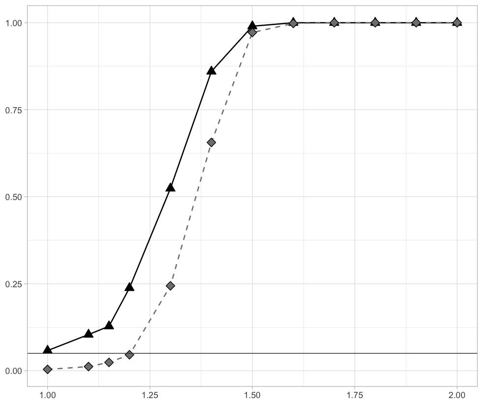
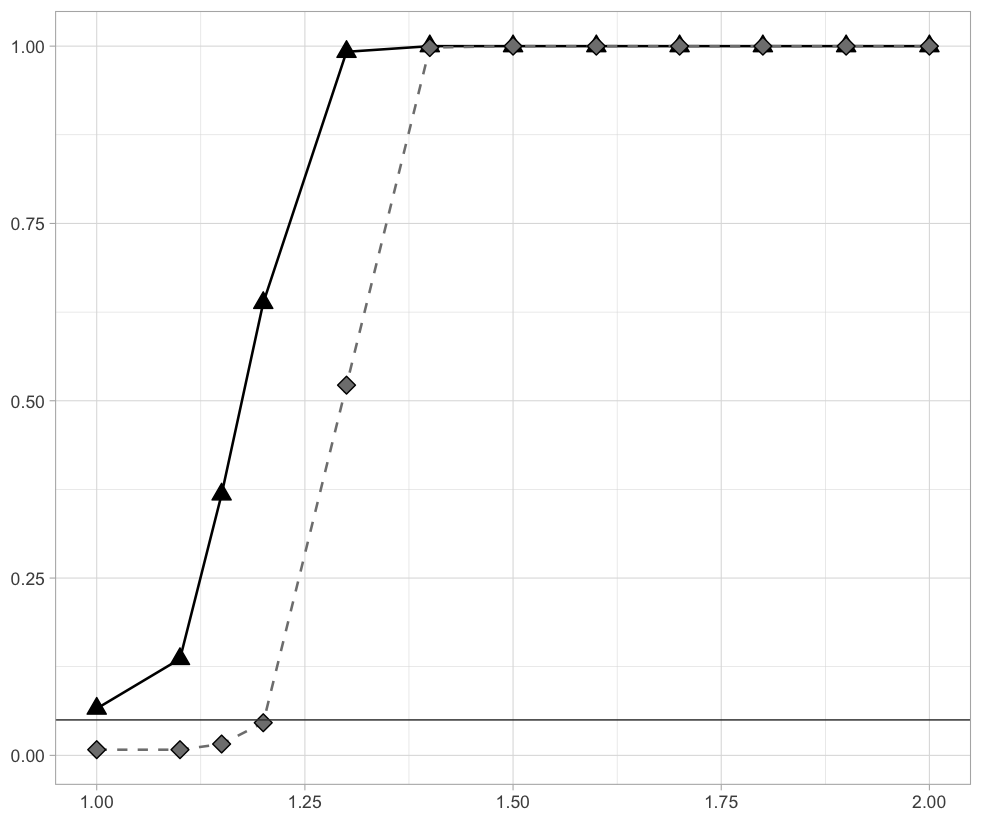
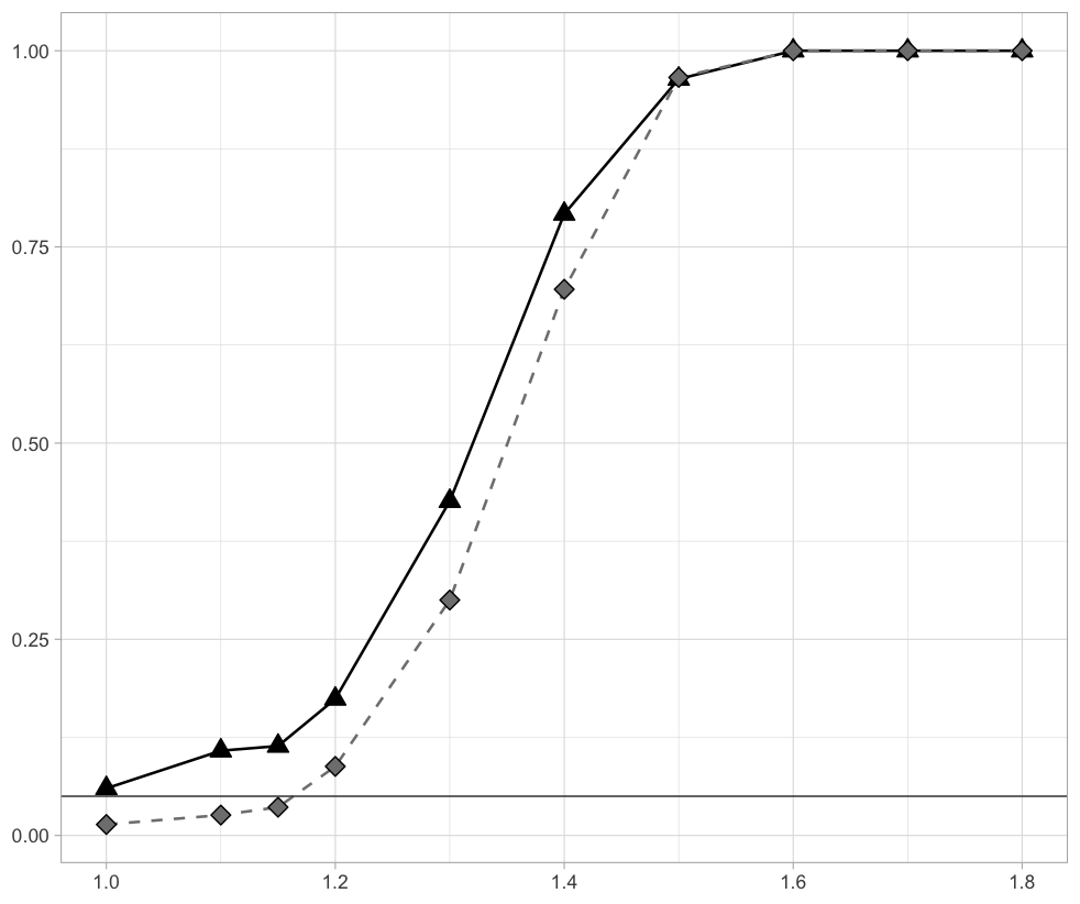
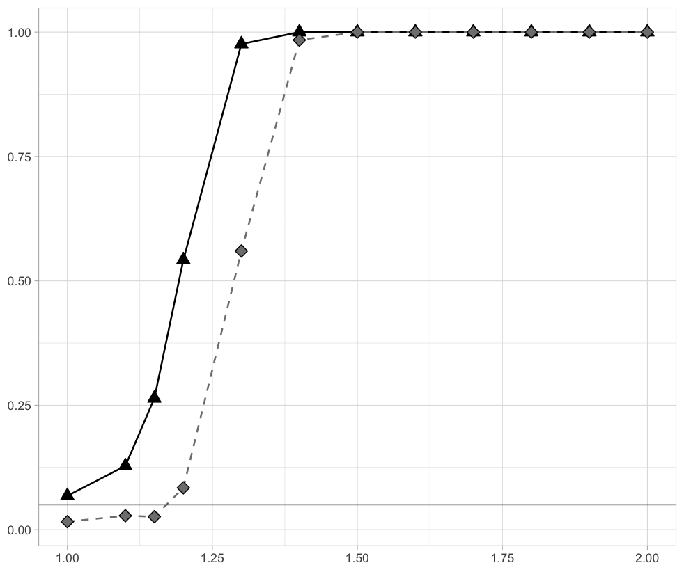
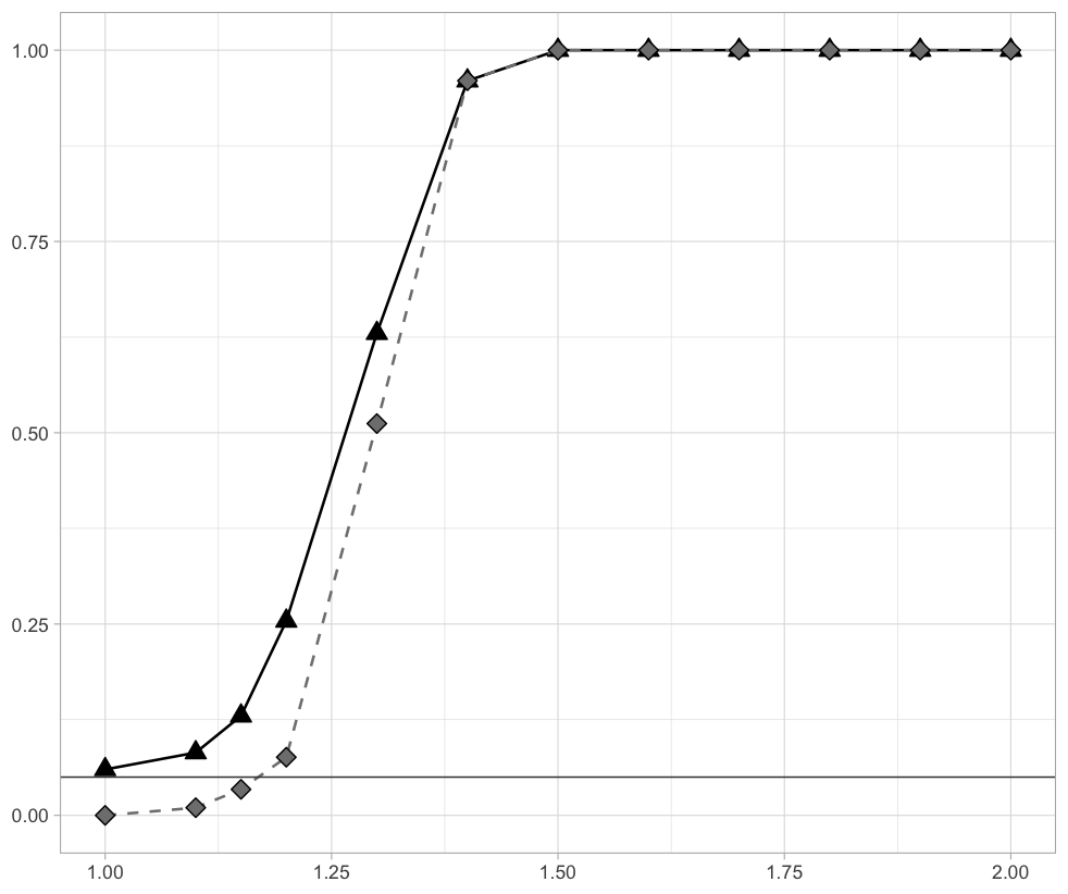
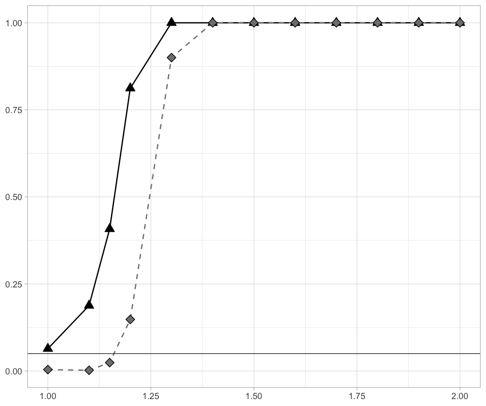
Figure 1: Empirical rejection rates of the new test (2.13) (triangle) compared to the test of Ryan and Killick (2023) (diamond), where $t_{0}=0.2,~{}t^{\star}=0.5$ and $(n,p)=(600,50)$ (first row), $(n,p)=(600,80)$ (middle row), $(n,p)=(800,100)$ (third row). Left panels: model (3.1)), where $x_{11}\sim{\cal N}(0,1)$. Right panels: model (3.2), where $x_{11}\sim\mathcal{U}(0,1)$.

3.3 Numerical experiments for the change-point estimation

In this section, we compare the new change point estimator $\hat{\tau}^{\star}$ in (2.16) with the estimators proposed by Aue et al. (2009) (AHHR) and Ryan and Killick (2023) (RK). All results are again based on $500$ simulation runs.

In Table 2, we compare the mean, standard deviation and mean squared error of the new estimator $\hat{\tau}^{\star}$ in (2.16) with the RK estimator for the different alternatives in model (3.1) (with $\mathcal{N}(0,1)$-distributed independent entries in the matrix $\mathbf{X}$), where $t^{\star}=0.5$, $(n,p)=(600,50)$ (top), $(n,p)=(600,80)$ (middle) and $(n,p)=(800,100)$ (bottom). Note that the dimension is of comparable magnitude to the sample size, and therefore, the AHHR estimator cannot be computed and is therefore not included in the comparison. For example, for a dimension $p=50$, one requires at least a sample size of $(p+1)p/2+1=1276$ to calculate this estimator (some results for the AHHR estimator can be found in Table 4). We observe from the upper part of Table 2 that the new estimator (2.16) outperforms the RK estimator in all three cases under consideration. The smaller mean squared error of the new estimator (2.16) is caused by both a smaller bias and variance. In particular, the RK estimator admits a significant bias for moderately strong signals $\delta\approx 1.5.$

In Table 3, we display the results of the two estimators for model (3.2) with uniformly distributed data. The results are similar to those presented in Table 2 for model (3.1). It is noteworthy that the new estimator performs well, even though the technical assumption (A4) is not satisfied. Again, our method outperforms the alternative RK approach in terms of smaller mean squared error.

We conclude this section with a small comparison of the two estimators $\hat{\tau}^{\star}$ and RK with the estimator proposed by Aue et al. (2009) (AHHR) in the model (3.1). For this purpose, we select $t^{\star}=0.4$, and display the characteristics of the three change point estimators in Table 4. Note that the AHHR estimator can only be computed if the sample size is at least $p(p+1)/2+1$ and for this reason, we consider the cases $(n,p)=(200,10)$ (top), $(n,p)=(200,15)$ (bottom). As the dimension is relatively small compared to the sample size, we choose $t_{0}=0.1$. We observe that, even in such cases, the estimator AHHR admits a significant bias resulting in a larger MSE compared to the other two methods. Interestingly, the bias of RK increases as the signal strength $\delta$ increases from moderately to large values. In contrast, the new estimator $\hat{\tau}^{\star}$ has decreasing bias and standard deviation as $\delta$ increases. Moreover, the new estimator always outperforms RK indicated by a smaller mean squared error, and AHHR in the case $(n,p)=(200,15).$ For $(n,p)=(200,10),$ we observe that the mean squared error of AHHR is smaller for weak signal strength $\delta.$ However, even for large $\delta$, this method admits a significant bias and is therefore outperformed by our method.

$\delta$		1.1	1.2	1.3	1.4	1.5	1.6	1.7	1.8	1.9	2
$\hat{\tau}^{\star}$	mean	0.499	0.499	0.506	0.493	0.496	0.494	0.497	0.496	0.499	0.499
	sd	0.123	0.112	0.091	0.066	0.054	0.034	0.025	0.018	0.010	0.008
	MSE	0.015	0.012	0.008	0.004	0.003	0.001	0.001	0.000	0.000	0.000
RK	mean	0.529	0.497	0.425	0.422	0.436	0.462	0.473	0.479	0.487	0.491
	sd	0.203	0.198	0.157	0.105	0.073	0.048	0.042	0.033	0.023	0.016
	MSE	0.042	0.039	0.030	0.017	0.009	0.004	0.002	0.001	0.001	0.000
$\hat{\tau}^{\star}$	mean	0.507	0.499	0.497	0.496	0.498	0.496	0.497	0.498	0.497	0.498
	sd	0.129	0.111	0.097	0.073	0.055	0.039	0.024	0.016	0.011	0.008
	MSE	0.017	0.012	0.009	0.005	0.003	0.002	0.001	0.000	0.000	0.000
RK	mean	0.515	0.501	0.420	0.395	0.413	0.431	0.450	0.460	0.468	0.474
	sd	0.211	0.210	0.161	0.096	0.074	0.058	0.044	0.040	0.033	0.026
	MSE	0.045	0.044	0.032	0.020	0.013	0.008	0.004	0.003	0.002	0.001
$\hat{\tau}^{\star}$	mean	0.495	0.495	0.494	0.494	0.496	0.498	0.499	0.499	0.499	0.500
	sd	0.124	0.106	0.082	0.055	0.038	0.023	0.013	0.010	0.006	0.005
	MSE	0.015	0.011	0.007	0.003	0.001	0.001	0.000	0.000	0.000	0.000
RK	mean	0.551	0.486	0.414	0.404	0.429	0.451	0.464	0.471	0.476	0.483
	sd	0.204	0.199	0.136	0.077	0.057	0.038	0.033	0.027	0.024	0.019
	MSE	0.044	0.040	0.026	0.015	0.008	0.004	0.002	0.002	0.001	0.001

Table 2: Simulated mean, standard deviation and mean squared error of the estimator $\hat{\tau}^{\star}$ in (2.16) and the estimator proposed in Ryan and Killick (2023) (RK), where $t_{0}=0.2,~{}t^{\star}=0.5$. The model is given by (3.1) with independent $\mathcal{N}(0,1)$-distributed entries in the matrix $\mathbf{X}$ and $(n,p)=(600,50)$ (top), $(n,p)=(600,80)$ (middle) and $(n,p)=(800,100)$ (bottom)

$\delta$		1.1	1.2	1.3	1.4	1.5	1.6	1.7	1.8	1.9	2
$\hat{\tau}^{\star}$	mean	0.507	0.499	0.498	0.496	0.498	0.500	0.499	0.500	0.500	0.500
	sd	0.123	0.087	0.055	0.033	0.009	0.006	0.004	0.003	0.003	0.001
	MSE	0.015	0.008	0.003	0.001	0.000	0.000	0.000	0.000	0.000	0.000
RK	mean	0.548	0.518	0.454	0.473	0.490	0.495	0.497	0.498	0.498	0.498
	sd	0.195	0.193	0.106	0.048	0.021	0.012	0.007	0.006	0.006	0.007
	MSE	0.040	0.037	0.013	0.003	0.001	0.000	0.000	0.000	0.000	0.000
$\hat{\tau}^{\star}$	mean	0.496	0.501	0.497	0.498	0.497	0.499	0.500	0.500	0.500	0.500
	sd	0.118	0.091	0.056	0.033	0.018	0.008	0.004	0.004	0.002	0.001
	MSE	0.014	0.008	0.003	0.001	0.000	0.000	0.000	0.000	0.000	0.000
RK	mean	0.548	0.505	0.428	0.458	0.481	0.490	0.495	0.496	0.497	0.498
	sd	0.198	0.199	0.109	0.052	0.032	0.019	0.010	0.008	0.008	0.005
	MSE	0.041	0.039	0.017	0.004	0.001	0.000	0.000	0.000	0.000	0.000
$\hat{\tau}^{\star}$	mean	0.495	0.501	0.499	0.501	0.499	0.499	0.500	0.500	0.500	0.500
	sd	0.106	0.075	0.036	0.015	0.007	0.006	0.001	0.002	0.001	0.001
	MSE	0.011	0.006	0.001	0.000	0.000	0.000	0.000	0.000	0.000	0.000
RK	mean	0.590	0.475	0.443	0.474	0.492	0.496	0.498	0.498	0.499	0.499
	sd	0.187	0.176	0.069	0.038	0.016	0.009	0.006	0.004	0.003	0.003
	MSE	0.043	0.032	0.008	0.002	0.000	0.000	0.000	0.000	0.000	0.000

Table 3: Simulated mean, standard deviation and mean squared error of the estimator $\hat{\tau}^{\star}$ in (2.16) and the estimator proposed in Ryan and Killick (2023) (RK), where $t_{0}=0.2,~{}t^{\star}=0.5$. The model is given by (3.2) with independent $\mathcal{U}(0,1)$-distributed entries in the matrix $\mathbf{X}$ and $(n,p)=(600,50)$ (top), $(n,p)=(600,80)$ (middle) and $(n,p)=(800,100)$ (bottom).

$\delta$		1.1	1.2	1.3	1.4	1.5	1.6	1.7	1.8	1.9	2
$\hat{\tau}^{\star}$	mean	0.497	0.491	0.475	0.452	0.446	0.428	0.421	0.415	0.415	0.407
	sd	0.167	0.152	0.150	0.133	0.124	0.111	0.081	0.080	0.066	0.048
	MSE	0.037	0.031	0.028	0.020	0.017	0.013	0.007	0.007	0.005	0.002
RK	mean	0.475	0.455	0.454	0.417	0.401	0.359	0.358	0.367	0.345	0.353
	sd	0.287	0.278	0.272	0.247	0.231	0.201	0.176	0.155	0.128	0.114
	MSE	0.088	0. 080	0.077	0.061	0.053	0.042	0.033	0.025	0.020	0.015
AHHR	mean	0.512	0.516	0.507	0.512	0.506	0.495	0.486	0.486	0.482	0.478
	sd	0.087	0.088	0.085	0.083	0.079	0.076	0.071	0.071	0.073	0.068
	MSE	0.020	0.021	0.019	0.019	0.017	0.015	0.012	0.012	0.012	0.011
$\hat{\tau}^{\star}$	mean	0.507	0.482	0.468	0.452	0.447	0.432	0.420	0.419	0.414	0.410
	sd	0.158	0.159	0.147	0.141	0.132	0.109	0.090	0.082	0.068	0.058
	MSE	0.036	0.032	0.026	0.022	0.020	0.013	0.009	0.007	0.005	0.003
RK	mean	0.483	0.463	0.451	0.409	0.407	0.379	0.365	0.358	0.354	0.355
	sd	0.294	0.301	0.293	0.275	0.255	0.237	0.211	0.196	0.183	0.165
	MSE	0.093	0.095	0.088	0.076	0.065	0.057	0.046	0.040	0.036	0.029
AHHR	mean	0.505	0.507	0.507	0.503	0.502	0.499	0.504	0.495	0.499	0.491
	sd	0.066	0.061	0.060	0.056	0.060	0.058	0.056	0.057	0.052	0.058
	MSE	0.015	0.015	0.015	0.014	0.014	0.013	0.014	0.012	0.012	0.012

Table 4: Estimated change point location given by $\hat{\tau}^{\star}$ compared to Ryan and Killick (2023) (RK) and Aue et al. (2009) (AHHR) under model (3.1) based on 500 simulation runs in the setting $(n,p)=(200,10)$ (top), $(n,p)=(200,15)$ (bottom), $t_{0}=0.1,~{}t^{\star}=0.4,x_{11}\sim\mathcal{N}(0,1)$.

4 Proofs of main results under the null hypothesis

4.1 Proof of Theorem 1

Throughout this section, we may assume $\mathbb{E}[x_{11}]=0$ by definition of $\Lambda_{n,t}^{\textnormal{cen}}$ without loss of generality. The first step in the proof of Theorem 1 consists of reducing it to a corresponding statement for the non-centered sample covariance matrix. For this purpose, we proceed with some preparations and define the non-centered sequential sample covariance matrices as

$$\hat{\mathbf{\Sigma}}_{i:j}^{(n)} =\hat{\mathbf{\Sigma}}_{i:j}=\frac{1}{j-i+1}\sum\limits_{k=i}^{j}\mathbf{y}_{j}\mathbf{y}_{j}^{\top},\quad 1\leq i\leq j\leq n,$$

$$\hat{\mathbf{\Sigma}} =\hat{\mathbf{\Sigma}}_{1:n}.$$

Consider the sequential likelihood ratio statistics

$$\Lambda_{n,t}=\frac{\big{|}\hat{\mathbf{\Sigma}}_{1:\lfloor nt\rfloor}\big{|}^{\frac{1}{2}\lfloor nt\rfloor}\big{|}\hat{\mathbf{\Sigma}}_{(\lfloor nt\rfloor+1):n}\big{|}^{\frac{1}{2}(n-\lfloor nt\rfloor)}}{\big{|}\hat{\mathbf{\Sigma}}\big{|}^{\frac{1}{2}n}},\quad t\in(0,1).$$ (4.1)

and the corresponding centered process

$$\mathbf{\Lambda}_{n}=((2\log\Lambda_{n,t}-\mu_{n,t})/n)_{t\in[t_{0},1-t_{0}]},$$

where the centering term is defined as

$$\mu_{n,t} =n\left(n-p-\frac{1}{2}\right)\log\Big{(}1-\frac{p}{n}\Big{)}-\lfloor nt\rfloor\left(\lfloor nt\rfloor-p-\frac{1}{2}\right)\log\Big{(}1-\frac{p}{\lfloor nt\rfloor}\Big{)}$$

$$\quad-(n-\lfloor nt\rfloor)\left(n-\lfloor nt\rfloor-p-\frac{1}{2}\right)\log\left(1-\frac{p}{n-\lfloor nt\rfloor}\right)+\frac{(\hat{\kappa}_{n}-3)p}{2},\quad t\in[t_{0},1-t_{0}].$$

In the following theorem, we provide the convergence of the finite-dimensional distributions of $(\mathbf{\Lambda}_{n})_{n\in\mathbb{N}}.$

Theorem 4.

Suppose that assumptions (A1), (A2) for some $\delta>0$, and (A3) are satisfied, and that $\mathbb{E}[x_{11}]=0$. For $n\to\infty$ and all fixed $k\in\mathbb{N}$, $t_{1},\ldots,t_{k}\in[t_{0},1-t_{0}]$, we have under $H_{0}$

$$\Big{(}\frac{2\log\Lambda_{n,t_{i}}-\mu_{n,t_{i}}}{n}\Big{)}_{1\leq i\leq k}\stackrel{{\scriptstyle\mathcal{D}}}{{\to}}(Z(t_{i}))_{1\leq i\leq k},$$

where $(Z(t))_{t\in[t_{0},1-t_{0}]}$ denotes the Gaussian process defined in Theorem 1.

The asymptotic tightness of $(\mathbf{\Lambda}_{n})_{n\in\mathbb{N}}$ is given in the next theorem.

Theorem 5.

Suppose that Assumptions (A1), (A2) with $\delta>4$ and (A3) are satisfied, and that $\mathbb{E}[x_{11}]=0$. Then, the sequence $(\mathbf{\Lambda}_{n})_{n\in\mathbb{N}}$ is asymptotically tight in the space $\ell^{\infty}([t_{0},1-t_{0}]).$

Proofs of these statements can be found in Section 4.1.1 and 4.1.3, respectively. Then, the weak convergence of $(\mathbf{\Lambda}_{n})_{n\in\mathbb{N}}$ towards a Gaussian process follows from the convergence of the finite-dimensional distributions (Theorem 4) and the tightness result (Theorem 5).

Corollary 2.

Suppose that assumptions (A1), (A2) with $\delta>4$, (A3) are satisfied, and that $\mathbb{E}[x_{11}]=0$. Then, we have under the null hypothesis $H_{0}$ of no change point

$$\Big{(}\frac{2\log\Lambda_{n,t}-\mu_{n,t}}{n}\Big{)}_{t\in[t_{0},1-t_{0}]}\stackrel{{\scriptstyle\mathcal{D}}}{{\to}}\big{(}Z(t)\big{)}_{t\in[t_{0},1-t_{0}]}\quad\textnormal{in }\ell^{\infty}([t_{0},1-t_{0}]),$$

where $(Z(t))_{t\in[t_{0},1-t_{0}]}$ denotes the centered Gaussian process defined in Theorem 1.

Before continuing with the proof of Theorem 1, we comment on the integration of our theoretical result in the existing line of literature.

Remark 2.

1. Theorem 1 and Corollary 2 continue the line of literature on substitution principles in random matrix theory. When considering the spectral statistics of $\hat{\mathbf{\Sigma}}$ and $\hat{\mathbf{\Sigma}}^{(\textnormal{cen})}$, it was found by Zheng, Bai and Yao (2015) that their asymptotic distributions are linked by a substitution principle. This results says that one needs to substitute the location parameter $c_{n}$ in the CLT for the linear spectral statistics of $\hat{\mathbf{\Sigma}}$ by $c_{n-1}$ to account for the centralization in $\hat{\mathbf{\Sigma}}^{\textnormal{cen}}.$ A similar result has been found by Yin, Zheng and Zou (2023) for the linear eigenvalue statistics of the sample correlation matrix. However, it is important to emphasize that the test statistic $\Lambda_{n,t}^{\textnormal{cen}}$ considered in this work is a functional of several strongly dependent eigenvalue statistics, and therefore these results are not applicable. In fact, the analysis of $\Lambda_{n,t}^{\textnormal{cen}}$ requires a careful study, accounting for its intricate structure. These challenges will be faced even when restricting our focus to the case of one-dimensional distributions of $(\Lambda_{n,t})_{t}$, let alone considering the process convergence.

2. For the process convergence of $(\mathbf{\Lambda}_{n})_{n\in\mathbb{N}}$ in the space of bounded functions, the stronger moments condition (A2) with $\delta>4$ is needed, whereas moments of order $4+\delta$ for some $\delta>0$ are sufficient for the convergence of the finite-dimensional distributions of $(\log\Lambda_{n,t})_{t\in[t_{0},1-t_{0}]}$.

With these preparations, we are in a position to prove Theorem 1.

Proof of Theorem 1.

Note that

$$\hat{\mathbf{\Sigma}}^{\textnormal{cen}}=\frac{n}{n-1}\hat{\mathbf{\Sigma}}-\overline{\mathbf{y}}\overline{\mathbf{y}}^{\top},$$

where $\overline{\mathbf{y}}=\overline{\mathbf{y}}_{1:n}$ denotes the sample mean of $\mathbf{y}_{1},\ldots,\mathbf{y}_{n}$. Using the matrix determinant lemma, this implies

$$\log|\hat{\mathbf{\Sigma}}^{\textnormal{cen}}| =\log\big{|}\frac{n}{n-1}\hat{\mathbf{\Sigma}}\big{|}+\log\left(1-\overline{\mathbf{y}}^{\top}\hat{\mathbf{\Sigma}}^{-1}\overline{\mathbf{y}}\right)$$

$$=-p\log\left(1-\frac{1}{n}\right)+\log\left|\hat{\mathbf{\Sigma}}\right|+\log\left(1-\overline{\mathbf{y}}^{\top}\hat{\mathbf{\Sigma}}^{-1}\overline{\mathbf{y}}\right).$$

A Taylor expansion shows that $-p\log\left(1-\frac{1}{n}\right)=p/n+o(1)$, and it also holds $\log\left(1-\overline{\mathbf{y}}^{\top}\hat{\mathbf{\Sigma}}^{-1}\overline{\mathbf{y}}\right)=\log(1-p/n)+o(1)$ almost surely (see Section 4.3.1 in Heiny and Parolya, 2023). Thus, we obtain

$$\log|\hat{\mathbf{\Sigma}}^{\textnormal{cen}}| =\log\left|\hat{\mathbf{\Sigma}}\right|+\frac{p}{n}+\log\left(1-\frac{p}{n}\right)+o(1)\quad\textnormal{almost surely}.$$ (4.2)

Similarly, one can show that

$$\log|\hat{\mathbf{\Sigma}}^{\textnormal{cen}}_{1:\lfloor nt\rfloor}| =\log\left|\hat{\mathbf{\Sigma}}_{1:\lfloor nt\rfloor}\right|+\frac{p}{\lfloor nt\rfloor}+\log\Big{(}1-\frac{p}{\lfloor nt\rfloor}\Big{)}+o(1)$$ (4.3)

$$\log|\hat{\mathbf{\Sigma}}^{\textnormal{cen}}_{(\lfloor nt\rfloor+1):n}| =\log\left|\hat{\mathbf{\Sigma}}_{(\lfloor nt\rfloor+1):n}\right|+\frac{p}{n-\lfloor nt\rfloor}+\log\Big{(}1-\frac{p}{n-\lfloor nt\rfloor}\Big{)}+o(1)$$ (4.4)

almost surely. Combining (4.2), (4.3) and (4.4), we can derive a representation of $\log\Lambda_{n,t}^{\textnormal{cen}}$ in terms of $\log\Lambda_{n,t}$, that is

$$\frac{2}{n}\log\Lambda_{n,t}^{\textnormal{cen}} =\frac{\lfloor nt\rfloor}{n}\log\left|\hat{\mathbf{\Sigma}}^{\textnormal{cen}}_{1:\lfloor nt\rfloor}\right|+\frac{n-\lfloor nt\rfloor}{n}\log\left|\hat{\mathbf{\Sigma}}^{\textnormal{cen}}_{(\lfloor nt\rfloor+1):n}\right|-\log\left|\hat{\mathbf{\Sigma}}^{\textnormal{cen}}\right|$$

$$=\frac{\lfloor nt\rfloor}{n}\log\left|\hat{\mathbf{\Sigma}}_{1:\lfloor nt\rfloor}\right|+\frac{n-\lfloor nt\rfloor}{n}\log\left|\hat{\mathbf{\Sigma}}_{(\lfloor nt\rfloor+1):n}\right|-\log\left|\hat{\mathbf{\Sigma}}\right|+\log\Big{(}1-\frac{p}{\lfloor nt\rfloor}\Big{)}$$

$$\quad+\log\Big{(}1-\frac{p}{n-\lfloor nt\rfloor}\Big{)}-\log\Big{(}1-\frac{p}{n}\Big{)}+\frac{p}{n}+o(1)$$

$$=\frac{2}{n}\log\Lambda_{n,t}+\log\Big{(}1-\frac{p}{\lfloor nt\rfloor}\Big{)}+\frac{n-\lfloor nt\rfloor}{n}\log\Big{(}1-\frac{p}{n-\lfloor nt\rfloor}\Big{)}$$

$$\quad-\frac{\lfloor nt\rfloor}{n}\log\left(1-\frac{p}{n}\right)+\frac{p}{n}+o(1).$$ (4.5)

Next, we find a more handy form for the centering term of $\log\Lambda_{n,t}^{\textnormal{cen}}$. As a preparation, we note that

$$\left(n-p-\frac{3}{2}\right)\left(\log\left(1-\frac{p}{n}\right)-\log\left(1-\frac{p}{n-1}\right)\right)=\frac{p}{n}+o(1),$$

which follows by a Taylor expansion. Then, we calculate

$$\frac{\mu_{n,t}}{n}+\log\Big{(}1-\frac{p}{\lfloor nt\rfloor}\Big{)}+\log\Big{(}1-\frac{p}{n-\lfloor nt\rfloor}\Big{)}-\log\left(1-\frac{p}{n}\right)+\frac{p}{n}$$

$$=\left(n-p-\frac{3}{2}\right)\log\left(1-\frac{p}{n}\right)-\frac{\lfloor nt\rfloor}{n}\left(\lfloor nt\rfloor-p-\frac{3}{2}\right)\log\left(1-\frac{p}{\lfloor nt\rfloor}\right)+\frac{(\hat{\kappa}_{n}-4)p}{2}$$

$$\quad-\frac{n-\lfloor nt\rfloor}{n}\left(n-\lfloor nt\rfloor-p-\frac{3}{2}\right)\log\Big{(}1-\frac{p}{n-\lfloor nt\rfloor}\Big{)}+\frac{p}{n}$$

$$= \left(n-p-\frac{3}{2}\right)\log\Big{(}1-\frac{p}{n-1}\Big{)}-\frac{\lfloor nt\rfloor}{n}\left(\lfloor nt\rfloor-p-\frac{3}{2}\right)\log\Big{(}1-\frac{p}{\lfloor nt\rfloor-1}\Big{)}$$

$$\quad-\frac{n-\lfloor nt\rfloor}{n}\left(n-\lfloor nt\rfloor-p-\frac{3}{2}\right)\log\Big{(}1-\frac{p}{n-\lfloor nt\rfloor-1}\Big{)}+\frac{(\hat{\kappa}_{n}-4)p}{2}+o(1)$$

$$=\tilde{\mu}_{n,t}+o(1),$$ (4.6)

where we note for later usage that the $o(1)$-term does not depend on $t\in[t_{0},1-t_{0}].$ By Theorem 4, (4.5) and (4.6), if follows that for all fixed $k\in\mathbb{N}$, $t_{1},\ldots,t_{k}\in[t_{0},1-t_{0}]$

$$\Big{(}\frac{2\log\Lambda_{n,t_{i}}^{\textnormal{cen}}-\tilde{\mu}_{n,t_{i}}}{n}\Big{)}_{1\leq i\leq k}\stackrel{{\scriptstyle\mathcal{D}}}{{\to}}(Z(t_{i}))_{1\leq i\leq k}.$$ (4.7)

Next, we aim to show that to show that

$$\Big{(}\frac{2\log\Lambda_{n,t}^{\textnormal{cen}}-\tilde{\mu}_{n,t}}{n}\Big{)}_{t\in[t_{0},1-t_{0}],n\in\mathbb{N}}$$ (4.8)

is asymptotically tight. Note that

$$\sup_{t\in[t_{0},1-t_{0}]}\Big{|}2\frac{\log\Lambda_{n,t}^{\textnormal{cen}}-\tilde{\mu}_{n,t}}{n}-2\frac{\log\Lambda_{n,t}-\mu_{n,t}}{n}\Big{|}$$

$$=\sup_{t\in[t_{0},1-t_{0}]}\Big{|}\log\Big{(}1-\frac{p}{\lfloor nt\rfloor}\Big{)}+\log\Big{(}1-\frac{p}{n-\lfloor nt\rfloor}\Big{)}-\log\left(1-\frac{p}{n}\right)+\frac{p}{n}\Big{|}+o(1)\lesssim 1$$ (4.9)

almost surely. By Theorem 5 and (4.9), we conclude that (4.8) is asymptotically tight. Combining this with (4.7), it follows from Theorem 1.5.4 on Van Der Vaart and Wellner (1996) that

$$\Big{(}\frac{2\log\Lambda_{n,t}^{\textnormal{cen}}-\tilde{\mu}_{n,t}}{n}\Big{)}_{t\in[t_{0},1-t_{0}]}\stackrel{{\scriptstyle\mathcal{D}}}{{\to}}\big{(}Z(t)\big{)}_{t\in[t_{0},1-t_{0}]}\quad\textnormal{in }\ell^{\infty}([t_{0},1-t_{0}]).$$

The proof of Theorem 1 concludes by an application of the continuous mapping theorem. ∎

4.1.1 Proof of Theorem 4 - weak convergence of finite-dimensional distributions

In the following, we prove Theorem 4, and the necessary auxiliary results are stated in Section 4.1.2.

Proof of Theorem 4.

For the sake of convenience, we restrict ourselves to the case $k=2.$ Then, using the Cramér–Wold theorem, it suffices to show that

$$a_{1}\frac{2\log\Lambda_{n,t_{1}}-\mu_{n,t_{1}}}{n}+a_{2}\frac{2\log\Lambda_{n,t_{2}}-\mu_{n,t_{2}}}{n}\stackrel{{\scriptstyle\mathcal{D}}}{{\to}}\mathcal{N}(0,\tau_{t_{1},t_{2}}^{2})$$

for $a_{1},a_{2}\in\mathbb{R},$ where $\tau_{t_{1},t_{2}}^{2}=\operatorname{Var}(a_{1}Z(t_{1})+a_{2}Z(t_{2})).$ In the following, we establish a useful representation of $2\log\Lambda_{n,t}$ by applying a QR-decomposition to several (sub)data matrices. For this purpose, we define for $1\leq i\leq j\leq n$ the matrices

$$\mathbf{X}_{i:j} =(\mathbf{x}_{i},\ldots,\mathbf{x}_{j})=(\mathbf{b}_{1,i:j},\ldots,\mathbf{b}_{p,i:j})^{\top}_{\in\mathbb{R}^{p\times(i-j+1)}},\quad\hat{\mathbf{I}}_{i:j}=\frac{1}{j-i+1}\mathbf{X}_{i:j}\mathbf{X}_{i:j}^{\top},\quad$$

$$\hat{\mathbf{I}} =\hat{\mathbf{I}}_{1:n},\quad\mathbf{b}_{i}=\mathbf{b}_{i,1:n}.$$

Moreover, let $\mathbf{P}(i;j:k)$ for $1\leq i\leq p$ and $1\leq j\leq k\leq n$ denote the projection matrix on the orthogonal complement of

$$\operatorname{span}\{\mathbf{b}_{1,j:k},\ldots,\mathbf{b}_{i,j:k}\},$$

that is, if we let $\mathbf{X}_{i,j:k}=(\mathbf{b}_{1,j:k},\ldots,\mathbf{b}_{i,j:k})^{\top}_{\in\mathbb{R}^{k\times(k-j+1)\times i}},$ then

$$\mathbf{P}(i;j:k)=\mathbf{I}-\mathbf{X}_{i,j:k}^{\top}\left(\mathbf{X}_{i,j:k}\mathbf{X}_{i,j:k}^{\top}\right)^{-1}\mathbf{X}_{i,j:k}$$

Note that $X_{i:j}=X_{p:i,j}$, set $\mathbf{P}(0;j:k)=\mathbf{I}$ and $\mathbf{P}(i;1:n)=\mathbf{P}(i).$ Before rewriting $\log\Lambda_{n,t}$, we need some preparations. By applying QR-decompositions to $\mathbf{X}_{1:\lfloor nt\rfloor}^{\top},~{}\mathbf{X}_{(\lfloor nt\rfloor+1):n}^{\top}$ and $\mathbf{X}_{n}^{\top}$ (see (Wang, Han and Pan, 2018, Section 2) for more details), respectively, we have

$$\left|n\hat{\mathbf{I}}\right| =\prod_{i=1}^{p}\mathbf{b}_{i}^{\top}\mathbf{P}(i-1)\mathbf{b}_{i},\quad$$

$$\left|\lfloor nt\rfloor\hat{\mathbf{I}}_{1:\lfloor nt\rfloor}\right| =\prod_{i=1}^{p}\mathbf{b}_{i,1:\lfloor nt\rfloor}^{\top}\mathbf{P}(i-1;1:\lfloor nt\rfloor)\mathbf{b}_{i,1:\lfloor nt\rfloor},\quad$$

$$\left|(n-\lfloor nt\rfloor)\hat{\mathbf{I}}_{(\lfloor nt\rfloor+1):n}\right| =\prod_{i=1}^{p}\mathbf{b}_{i,(\lfloor nt\rfloor+1):n}^{\top}\mathbf{P}(i-1;(\lfloor nt\rfloor+1):n)\mathbf{b}_{i,(\lfloor nt\rfloor+1):n}.$$

Thus, under the null hypothesis of no change point, the likelihood ratio statistic does not depend on $\mathbf{\Sigma}$ and we may write

$$2\log\Lambda_{n,t} =2\log\frac{\left|\hat{\mathbf{I}}_{1:\lfloor nt\rfloor}\right|^{\frac{1}{2}\lfloor nt\rfloor}\left|\hat{\mathbf{I}}_{(\lfloor nt\rfloor+1):n}\right|^{\frac{1}{2}(n-\lfloor nt\rfloor)}}{\left|\hat{\mathbf{I}}\right|^{\frac{1}{2}n}}$$

$$=\lfloor nt\rfloor\log\left|\hat{\mathbf{I}}_{1:\lfloor nt\rfloor}\right|+(n-\lfloor nt\rfloor)\log\left|\hat{\mathbf{I}}_{(\lfloor nt\rfloor+1):n}\right|-n\log\left|\hat{\mathbf{I}}\right|$$

$$=\lfloor nt\rfloor\log\left|\lfloor nt\rfloor\hat{\mathbf{I}}_{1:\lfloor nt\rfloor}\right|+(n-\lfloor nt\rfloor)\log\left|(n-\lfloor nt\rfloor)\hat{\mathbf{I}}_{(\lfloor nt\rfloor+1):n}\right|-n\log\left|n\hat{\mathbf{I}}\right|$$ (4.10)

$$\quad+np\log n-\lfloor nt\rfloor p\log\lfloor nt\rfloor-(n-\lfloor nt\rfloor)p\log(n-\lfloor nt\rfloor).$$

$$=\lfloor nt\rfloor\sum_{i=1}^{\lfloor nt\rfloor}\log\mathbf{b}_{i,1:\lfloor nt\rfloor}^{\top}\mathbf{P}(i-1;1:\lfloor nt\rfloor)\mathbf{b}_{i,1:\lfloor nt\rfloor}$$

$$+(n-\lfloor nt\rfloor)\sum_{i=\lfloor nt\rfloor+1}^{n}\log\mathbf{b}_{i,(\lfloor nt\rfloor+1):n}^{\top}\mathbf{P}(i-1;(\lfloor nt\rfloor+1):n)\mathbf{b}_{i,(\lfloor nt\rfloor+1):n}$$

$$-n\sum_{i=1}^{n}\log\mathbf{b}_{i}^{\top}\mathbf{P}(i-1)\mathbf{b}_{i}+np\log n-\lfloor nt\rfloor p\log\lfloor nt\rfloor-(n-\lfloor nt\rfloor)p\log(n-\lfloor nt\rfloor).$$ (4.11)

Next, we define for $1\leq i\leq p$ and $t\in\{t_{1},t_{2}\}$

$$X_{i} =\frac{\mathbf{b}_{i}^{\top}\mathbf{P}(i-1)\mathbf{b}_{i}-(n-i+1)}{n-i+1},$$ (4.12)

$$X_{i,1:\lfloor nt\rfloor} =\frac{\mathbf{b}_{i,1:\lfloor nt\rfloor}^{\top}\mathbf{P}(i-1;1:\lfloor nt\rfloor)\mathbf{b}_{i,1:\lfloor nt\rfloor}-(\lfloor nt\rfloor-i+1)}{\lfloor nt\rfloor-i+1},$$ (4.13)

$$X_{i,(\lfloor nt\rfloor+1):n} =\frac{\mathbf{b}_{i,(\lfloor nt\rfloor+1):n}^{\top}\mathbf{P}(i-1;(\lfloor nt\rfloor+1):n)\mathbf{b}_{i,(\lfloor nt\rfloor+1):n}-(n-\lfloor nt\rfloor-i+1)}{n-\lfloor nt\rfloor-i+1},$$

$$Y_{i} =\log(1+X_{i})-\Big{(}X_{i}-\frac{X_{i}^{2}}{2}\Big{)},$$ (4.14)

$$Y_{i,j:k} =\log(1+X_{i,j:k})-\Big{(}X_{i,j:k}-\frac{X_{i,j:k}^{2}}{2}\Big{)},\quad 1\leq j\leq k\leq n.$$ (4.15)

Using Stirling’s formula

$$\log n!=n\log n-n+\frac{1}{2}\log(2\pi n)+\frac{1}{12n}+\mathcal{O}\left(n^{-3}\right),\quad n\to\infty,$$

a straightforward calculation gives

$$\sum_{i=1}^{p}\lfloor nt\rfloor\log(\lfloor nt\rfloor-i+1)+\sum_{i=1}^{p}(n-\lfloor nt\rfloor)\log(n-\lfloor nt\rfloor-i+1)-n\sum_{i=1}^{p}\log(n-i+1)$$

$$\quad+np\log n-\lfloor nt\rfloor p\log\lfloor nt\rfloor-(n-\lfloor nt\rfloor)p\log(n-\lfloor nt\rfloor)$$

$$=\mu_{n,t}+\frac{n\breve{\sigma}_{n,t}^{2}}{2}+o(n),\quad n\to\infty,$$ (4.16)

where

$$n\breve{\sigma}_{n,t}^{2}=2n\log\left(1-\frac{p}{n}\right)-2\lfloor nt\rfloor\log\Big{(}1-\frac{p}{\lfloor nt\rfloor}\Big{)}-2(n-\lfloor nt\rfloor)\log\Big{(}1-\frac{p}{n-\lfloor nt\rfloor}\Big{)}-(\hat{\kappa}_{n}-3)p.$$ (4.17)

Combining (4.11) and (4.16) gives the representation

$$a_{1}\left(2\log\Lambda_{n,t_{1}}-\mu_{n,t_{1}}\right)+a_{2}\left(2\log\Lambda_{n,t_{2}}-\mu_{n,t_{2}}\right)$$

$$=\sum_{j=1,2}\Bigg{\{}a_{j}\sum_{i=1}^{p}\lfloor nt_{j}\rfloor X_{i,1:\lfloor nt_{j}\rfloor}+a_{j}\sum_{i=1}^{p}(n-\lfloor nt_{j}\rfloor)X_{i,(\lfloor nt_{j}\rfloor+1):n}-a_{j}n\sum_{i=1}^{p}X_{i}$$

$$\quad-a_{j}\left(\sum_{i=1}^{p}\lfloor nt_{j}\rfloor\frac{X_{i,1:\lfloor nt_{j}\rfloor}}{2}^{2}+(n-\lfloor nt_{j}\rfloor)\frac{X_{i,(\lfloor nt_{j}\rfloor+1):n}^{2}}{2}-n\sum_{i=1}^{p}\frac{X_{i}^{2}}{2}-\frac{n\breve{\sigma}_{n,t_{j}}^{2}}{2}\right)$$

$$\quad+a_{j}\sum_{i=1}^{p}\lfloor nt_{j}\rfloor Y_{i,1:\lfloor nt_{j}\rfloor}+a_{j}\sum_{i=1}^{p}(n-\lfloor nt_{j}\rfloor)Y_{i,(\lfloor nt_{j}\rfloor+1):n}-a_{j}n\sum_{i=1}^{p}Y_{i}\Bigg{\}}+o(n)$$

$$=\sum_{j=1,2}\Bigg{\{}a_{j}\sum_{i=1}^{p}\lfloor nt_{j}\rfloor X_{i,1:\lfloor nt_{j}\rfloor}+a_{j}\sum_{i=1}^{p}(n-\lfloor nt_{j}\rfloor)X_{i,(\lfloor nt_{j}\rfloor+1):n}-a_{j}n\sum_{i=1}^{p}X_{i}\Bigg{\}}+o_{\mathbb{P}}(n),$$

where we applied Lemma 2 and Lemma 1 for the last estimate, which are given in Section 4.1.2 below. Defining

$$D_{i} =\sum_{j=1,2}a_{j}D_{i,j},$$

$$D_{i,j} =\lfloor nt_{j}\rfloor X_{i,1:\lfloor nt_{j}\rfloor}+(n-\lfloor nt_{j}\rfloor)X_{i,(\lfloor nt_{j}\rfloor+1):n}-nX_{i},\quad 1\leq i\leq p,$$ (4.18)

it remains to show that

$$\frac{1}{n}\sum_{i=1}^{p}D_{i}\stackrel{{\scriptstyle\mathcal{D}}}{{\to}}\mathcal{N}(0,\tau_{t_{1},t_{2}}^{2}).$$ (4.19)

Note that $(D_{i}/n)_{1\leq i\leq p}$ forms a martingale difference scheme with respect to filtration $(\mathcal{A}_{i})_{1\leq i\leq p}$, where the $\sigma$-field $\mathcal{A}_{i}$ is generated by the random variables $\mathbf{b}_{1},\ldots,\mathbf{b}_{i}$ for $1\leq i\leq p.$ In the following, we will show that

$$\sum_{i=1}^{p}\mathbb{E}\left[\frac{D_{i,1}D_{i,2}}{n^{2}}\Big{|}\mathcal{A}_{i-1}\right] =\operatorname{cov}(Z(t_{1}),Z(t_{2}))+o_{\mathbb{P}}(1),$$ (4.20)

$$\sum_{i=1}^{p}\mathbb{E}\left[D_{i,j}^{2}I\{|D_{i,,j}|>\varepsilon\}\right] =o_{\mathbb{P}}(1),\quad j=1,2,$$ (4.21)

By the CLT for martingale differences (see, for example, Corollary 3.1 in Hall and Heyde, 1980), these statements imply (4.19). Regarding (4.21), we have, by Lemma B.26 in Bai and Silverstein (2010), for $\varepsilon>0$

$$\mathbb{E}\left|\sum_{i=1}^{p}\mathbb{E}[X_{i,1:\lfloor nt\rfloor}^{2}I\{|X_{i,1:\lfloor nt\rfloor}|>\varepsilon\}|\mathcal{A}_{i-1}]\right| \lesssim\frac{1}{\varepsilon^{\delta/2}}\sum_{i=1}^{p}\mathbb{E}\left|X_{i,1:\lfloor nt\rfloor}\right|^{2+\delta/2}$$

$$\lesssim\sum_{i=1}^{p}\frac{1}{(\lfloor nt\rfloor-i+1)^{1+\delta/4}}=o(1).$$

The other terms in $D_{i,j}$ can be bounded similarly and we (4.21) follows. Next we concentrate on the calculation of the covariance kernel in (4.20). We define for $1\leq j_{1}\leq j_{2}\leq k_{2}\leq k_{1}$ (such that $k_{l}-j_{l}-p>0$ for $l=1,2$

$$\mathbf{P}^{j_{2}:k_{2}}(i-1;j_{1}:k_{1})=\left(\left(\mathbf{P}(i-1;j_{1}:k_{1})\right)_{k,l}\right)_{j_{2}\leq k,l\leq k_{2}}\in\mathbb{R}^{(k_{2}-j_{2}+1)\times(k_{2}-j_{2}+1)}.$$ (4.22)

In particular, we have $\mathbf{P}^{j_{1}:k_{1}}(i-1;j_{1}:k_{1})=\mathbf{P}(i-1;j_{1}:k_{1})$ and

$$\operatorname{tr}\left(\mathbf{P}^{j_{2}:k_{2}}(i-1;j_{1}:k_{1})\mathbf{P}(i-1;j_{2}:k_{2})\right)=(k_{2}-j_{2}-i+1).$$

Using formula (9.8.6) in Bai and Silverstein (2010) we calculate for integers $j_{1},j_{2},k_{1},k_{2}$ such that $(k_{1}\wedge k_{2})-(j_{1}\vee j_{2})-p>0$ for $l=1,2$

$$n^{2}\sigma^{2}(j_{1},k_{1},j_{2},k_{2}):=\sum_{i=1}^{p}(k_{1}-j_{1}+1)(k_{2}-j_{2}+1)\mathbb{E}\left[X_{i,j_{1}:k_{1}}X_{i,j_{2}:k_{2}}\big{|}\mathcal{A}_{i-1}\right]$$

$$=\sum_{i=1}^{p}\frac{(k_{1}-j_{1}+1)(k_{2}-j_{2}+1)}{(k_{1}-j_{1}-i+1)(k_{2}-j_{2}-i+1)}\mathbb{E}\Big{[}\prod_{l=1,2}\left\{\mathbf{b}_{i,j_{l}:k_{l}}^{\top}\mathbf{P}(i-1;j_{l}:k_{l})\mathbf{b}_{i,j_{l}:k_{l}}-(k_{l}-j_{l}-i+1)\right\}\big{|}\mathcal{A}_{i-1}\Big{]}$$

$$=n^{2}\sigma_{1}^{2}(j_{1},k_{1},j_{2},k_{2})+(\mathbb{E}[x_{11}^{4}]-3)n^{2}\sigma_{2}^{2}(j_{1},k_{1},j_{2},k_{2}),$$ (4.23)

where

$$n^{2}\sigma_{1}^{2}(j_{1},k_{1},j_{2},k_{2}) =2\sum_{i=1}^{p}\frac{(k_{1}-j_{1}+1)(k_{2}-j_{2}+1)}{(k_{1}-j_{1}-i+1)\vee(k_{2}-j_{2}-i+1)}$$

$$\quad\quad\times\operatorname{tr}\left(\mathbf{P}^{(j_{1}\vee j_{2}):(k_{1}\wedge k_{2})}(i-1;j_{1}:k_{1})\mathbf{P}^{(j_{1}\vee j_{2}):(k_{1}\wedge k_{2})}(i-1;j_{2}:k_{2})\right),$$

$$n^{2}\sigma_{2}^{2}(j_{1},k_{1},j_{2},k_{2}) =\sum_{i=1}^{p}\frac{(k_{1}-j_{1}+1)(k_{2}-j_{2}+1)}{(k_{1}-j_{1}-i+1)(k_{2}-j_{2}-i+1)}$$

$$\quad\quad\times\operatorname{tr}\left(\mathbf{P}^{(j_{1}\vee j_{2}):(k_{1}\wedge k_{2})}(i-1;j_{1}:k_{1})\odot\mathbf{P}^{(j_{1}\vee j_{2}):(k_{1}\wedge k_{2})}(i-1;j_{2}:k_{2})\right)$$

and ${}^{\prime}\odot^{\prime}$ denotes the Hadamard product. We will evaluate these expressions in the case, where $k_{1}$ and $k_{2}$ (and maybe also $j_{1},j_{2}$) are proportional to $n$ using the expansion for the partial sums of the harmonic series

$$\sum_{k=1}^{n}\frac{1}{k}=\log n+\gamma+\mathcal{O}\left(\frac{1}{n}\right),\quad n\to\infty,$$

(where $\gamma$ denotes the Euler-Mascheroni constant). Using this estimate and (4.22), we obtain for $k_{2}-j_{2}+1=(k_{1}-j_{1}+1)\vee(k_{2}-j_{2}+1)$

$$\sigma_{1}^{2}(j_{1},k_{1},j_{2},k_{2}) =2\sum_{i=1}^{p}\frac{(k_{1}-j_{1}+1)(k_{2}-j_{2}+1)}{n^{2}(k_{2}-j_{2}-i+1)}$$

$$=2\frac{(k_{1}-j_{1}+1)(k_{2}-j_{2}+1)}{n^{2}}\sum_{i=k_{2}-j_{2}-p+1}^{k_{2}-j_{2}}\frac{1}{i}$$

$$=2\frac{(k_{1}-j_{1}+1)(k_{2}-j_{2}+1)}{n^{2}}\Big{\{}\sum_{i=1}^{k_{2}-j_{2}}\frac{1}{i}-\sum_{i=1}^{k_{2}-j_{2}-p}\frac{1}{i}\Big{\}}$$

$$=-2\frac{(k_{1}-j_{1}+1)(k_{2}-j_{2}+1)}{n^{2}}\log\Big{(}1-\frac{p}{k_{2}-j_{2}}\Big{)}+o(1)$$

$$=-2\frac{(k_{1}-j_{1}+1)(k_{2}-j_{2}+1)}{n^{2}}\log\Big{(}1-\frac{p}{(k_{1}-j_{1})\vee(k_{2}-j_{2})}\Big{)}+o(1).$$ (4.24)

For later use, we note that the $o(1)$ term in (4.24) does not depend on $t\in[t_{0},1-t_{0}]$, if we set $j_{1}=j_{2}=1,k_{1}=k_{2}=\lfloor nt\rfloor$ or $j_{1}=j_{2}=\lfloor nt\rfloor+1,k_{1}=k_{2}=n.$ Moreover, in the case $k_{2}-j_{2}+1=(k_{1}-j_{1}+1)\vee(k_{2}-j_{2}+1)$, it follows from Lemma 3 in Section 4.1.2 below that

$$\sigma_{2}^{2}(j_{1},k_{1},j_{2},k_{2}) =y\frac{k_{1}-j_{1}+1}{n}+o_{\mathbb{P}}(1),$$

$$\sigma_{2}^{2}(\lfloor nt_{1}\rfloor+1,n,1,\lfloor nt_{2}\rfloor) =y(t_{2}-t_{1})+o_{\mathbb{P}}(1).$$ (4.25)

To calculate $\operatorname{cov}(Z(t_{1}),Z(t_{2}))$ using (4.24), we use that $\sigma^{2}(j_{1},k_{1},j_{2},k_{2})=0$ if $1\leq j_{1}\leq k_{1}<j_{2}\leq k_{2}\leq n$ (this corresponds to the case that $X_{i,j_{1}:k_{1}}$ and $X_{i,j_{2}:k_{2}}$ are independent and thus $\mathbb{E}[X_{i,j_{1}:k_{1}}X_{i,j_{2}:k_{2}}|\mathcal{A}_{i-1}]=0$ for all $1\leq i\leq p$. ). In the following, we assume that $t_{1}<t_{2}$, which implies $\sigma^{2}(1,\lfloor nt_{1}\rfloor,\lfloor nt_{2}\rfloor+1,n)=0$. Combining (4.23) and (4.25) gives

$$\sum_{i=1}^{p}\mathbb{E}\left[\frac{D_{i,1}D_{i,2}}{n^{2}}\Big{|}\mathcal{A}_{i-1}\right]$$

$$=-\sigma^{2}(1,\lfloor nt_{1}\rfloor,1,n)+\sigma^{2}(1,\lfloor nt_{1}\rfloor,1,\lfloor nt_{2}\rfloor)+\sigma^{2}(1,\lfloor nt_{1}\rfloor,\lfloor nt_{2}\rfloor+1,n)$$

$$\quad-\sigma^{2}(\lfloor nt_{1}\rfloor+1,n,1,n)+\sigma^{2}(\lfloor nt_{1}\rfloor+1,n,1,\lfloor nt_{2}\rfloor)+\sigma^{2}(\lfloor nt_{1}\rfloor+1,n,\lfloor nt_{2}\rfloor+1,n)$$

$$\quad+\sigma^{2}(1,n,1,n)-\sigma^{2}(1,\lfloor nt_{2}\rfloor,1,n)-\sigma^{2}(\lfloor nt_{2}\rfloor+1,n,1,n)+o_{\mathbb{P}}(1)$$

$$=-\sigma_{1}^{2}(1,\lfloor nt_{1}\rfloor,1,n)+\sigma_{1}^{2}(1,\lfloor nt_{1}\rfloor,1,\lfloor nt_{2}\rfloor)-\sigma_{1}^{2}(\lfloor nt_{1}\rfloor+1,n,1,n)$$

$$\quad+\sigma_{1}^{2}(\lfloor nt_{1}\rfloor+1,n,1,\lfloor nt_{2}\rfloor)+\sigma_{1}^{2}(\lfloor nt_{1}\rfloor+1,n,\lfloor nt_{2}\rfloor+1,n)$$

$$\quad+\sigma_{1}^{2}(1,n,1,n)-\sigma_{1}^{2}(1,\lfloor nt_{2}\rfloor,1,n)-\sigma_{1}^{2}(\lfloor nt_{2}\rfloor+1,n,1,n)+o_{\mathbb{P}}(1).$$

Here, we used (4.25) to see that the contributions of the $\sigma_{2}^{2}$-terms cancel each other out. Next, we use Lemma 4 in Section 4.1.2 below to compute the term $\sigma_{1}^{2}(\lfloor nt_{1}\rfloor+1,n,1,\lfloor nt_{2}\rfloor)$. For all remaining $\sigma_{1}^{2}$-terms, we use (4.24) and obtain

$$\sum_{i=1}^{p}\mathbb{E}\left[\frac{D_{i,1}D_{i,2}}{n^{2}}\Big{|}\mathcal{A}_{i-1}\right]$$

$$=2t_{1}\log(1-y)-2t_{1}t_{2}\log\Big{(}1-y/t_{2}\Big{)}+2(1-t_{1})\log(1-y)$$

$$\quad-2(1-t_{1})t_{2}\log\left(1-\frac{(t_{2}-t_{1})y}{(1-t_{1})t_{2}}\right)-2(1-t_{1})(1-t_{2})\log(1-y/(1-t_{1}))$$

$$\quad-2\log(1-y)+2t_{2}\log(1-y)+2(1-t_{2})\log(1-y)$$

$$=2\log(1-y)-2t_{1}t_{2}\log(1-y/t_{2})-2(1-t_{1})t_{2}\log\Big{(}1-\frac{(t_{2}-t_{1})y}{(1-t_{1})t_{2}}\Big{)}$$

$$\quad-2(1-t_{1})(1-t_{2})\log(1-y/(1-t_{1}))+o_{\mathbb{P}}(1)$$

$$=\operatorname{cov}(Z(t_{1}),Z(t_{2}))+o_{\mathbb{P}}(1).$$

If $t_{1}=t_{2}=t$ , then we get

$$\operatorname{Var}(Z(t))=2\log(1-y)-2t^{2}\log(1-y/t)-2(1-t)^{2}\log(1-y/(1-t)).$$

∎

4.1.2 Auxiliary results for the proof of Theorem 4

The convergence of the finite-dimensional distributions is facilitated by the following auxiliary results, whose proofs are postponed to the supplementary material. To begin with, we have an result on the quadratic term appearing in the expansion of the test statistic.

Lemma 1.

As $n\to\infty,$ it holds for $t\in[t_{0},1-t_{0}]$

$$\sum_{i=1}^{p}\frac{\lfloor nt\rfloor}{n}\frac{X_{i,1:\lfloor nt\rfloor}}{2}^{2}+\frac{n-\lfloor nt\rfloor}{n}\sum_{i=1}^{p}\frac{X_{i,(\lfloor nt\rfloor+1):n}^{2}}{2}-\sum_{i=1}^{p}\frac{X_{i}^{2}}{2}-\frac{\breve{\sigma}_{n,t}^{2}}{2}=o_{\mathbb{P}}(1),$$

where $\breve{\sigma}^{2}_{n,t}$ is defined in (4.17).

The following result shows that the logarithmic terms are negligible at a $\delta$-dependent rate. It will also be used in Section 4.1.3 when the proving the asymptotic tightness given in Theorem 5.

Lemma 2.

Assume that (A1) and (A2) with some $\delta>0$ are satisfied. Then, it holds for all $t\in[t_{0},1-t_{0}]$

$$\frac{1}{n}\sum_{i=1}^{p}\left(\mathbb{E}\left|\lfloor nt\rfloor Y_{i,1:\lfloor nt\rfloor}\right|+\mathbb{E}\left|(n-\lfloor nt\rfloor)Y_{i,(\lfloor nt\rfloor+1):n}\right|+\mathbb{E}\left|nY_{i}\right|\right)\lesssim\frac{1}{n^{\delta/4}},$$

where the upper bound does not depend on $t$ and the random variables $Y_{i}$ and $Y_{i,(\lfloor nt\rfloor+1):n}$ are defined in (4.14) and (4.15), respectively.

In the following lemma, we provide an approximation for $\sigma_{2}^{2}$ appearing in (4.25).

Lemma 3.

Suppose that $p<j_{1}\leq j_{2}\leq k_{1}\leq k_{2}\leq n$ such that $k_{2}-j_{2}+1=(k_{1}-j_{1}+1)\vee(k_{2}-j_{2}+1)$. It holds

$$\sigma_{2}^{2}(j_{1},k_{1},j_{2},k_{2}) =y\frac{k_{1}-j_{1}+1}{n}+o_{\mathbb{P}}(1),$$

Moreover, we have for $t_{0}\leq t_{1}<t_{2}\leq t_{0}$

$$\sigma_{2}^{2}(\lfloor nt_{1}\rfloor+1,n,1,\lfloor nt_{2}\rfloor) =y(t_{2}-t_{1})+o_{\mathbb{P}}(1).$$

We conclude this section by an approximation of $\sigma_{1}^{2}$ defined below (4.23).

Lemma 4.

If $t_{1}<t_{2}$, then we have

$$\sigma_{1}^{2}(\lfloor nt_{1}\rfloor+1,n,1,\lfloor nt_{2}\rfloor)=-2(1-t_{1})t_{2}\log\left(1-\frac{(t_{2}-t_{1})y}{(1-t_{1})t_{2}}\right)+o_{\mathbb{P}}(1).$$

4.1.3 Proof of Theorem 5 - asymptotic tightness of $(\mathbf{\Lambda}_{n})_{n\in\mathbb{N}}$

We need the following auxiliary results, whose proofs are provided in Section A.5. To begin with, we investigate the increments of the contributing random part of $\log\Lambda_{n,t}$, which is shown to satisfy a finite-dimensional CLT in the proof of Theorem 4.

Lemma 5.

Let Assumption (A1) and (A2) with some $\delta>0$ be satisfied and let $t_{1},t_{2}\in[t_{0},1-t_{0}]$ and $D_{i,j}$ be defined as in (4.18) for $j\in\{1,2\},~{}1\leq i\leq p.$ Then, there exists random variables $Z_{1}=Z_{1,n}(t_{1},t_{2}),Z_{2}=Z_{2,n}(t_{1},t_{2})$ such that

$$\frac{1}{n}\sum\limits_{i=1}^{p}\left(D_{i,1}-D_{i,2}\right)=Z_{1}+Z_{2}$$

and

$$\mathbb{E}[Z_{1}^{2}] \lesssim\left|\frac{\lfloor nt_{1}\rfloor-\lfloor nt_{2}\rfloor}{n}\right|^{1+d}$$

$$\mathbb{E}[|Z_{2}|^{2+\delta/2}] \lesssim\left|\frac{\lfloor nt_{1}\rfloor-\lfloor nt_{2}\rfloor}{n}\right|^{1+d},$$

for some $d>0.$

Next, we need a uniform result on the quadratic terms, which is provided in the next lemma.

Lemma 6.

If Assumption (A1) and (A2) with some $\delta>4$ are satisfied, then there exist random variables $Q_{n,1,t}$ and $Q_{n,2,t}$ with

$$Q_{n,1,t}+Q_{n,2,t}=\sum_{i=1}^{p}\frac{\lfloor nt\rfloor}{n}\frac{X_{i,1:\lfloor nt\rfloor}}{2}^{2}+\frac{n-\lfloor nt\rfloor}{n}\sum_{i=1}^{p}\frac{X_{i,(\lfloor nt\rfloor+1):n}^{2}}{2}-\sum_{i=1}^{p}\frac{X_{i}^{2}}{2}-\frac{\breve{\sigma}_{n,t}^{2}}{2},$$ (4.26)

such that $(Q_{n,1,t})$ is asymptotically tight in $\ell^{\infty}([t_{0},1-t_{0}])$ and $(Q_{2,n,t})$ satisfies the moment inequality

$$\sup_{t\in[t_{0},1-t_{0}]}\mathbb{E}|Q_{2,n,t}|^{2+\delta/4}\lesssim\frac{1}{n^{1+\delta/8}}.$$ (4.27)

Finally, we recall Lemma 2 given in Section 4.1.2 on the logarithmic terms. Using these auxiliary results, we are in the position to give a proof of Theorem 5.

Proof of Theorem 5.

By Lemma 6 and (4.16), it suffices to show that $\{L_{n,t_{1}}\}_{t_{1}\in[t_{0},1-t_{0}]}$ with

$$L_{n,t_{1}}:=\frac{1}{n}\sum_{i=1}^{p}D_{i,1}-Q_{2,n,t_{1}}+\sum_{i=1}^{p}\frac{\lfloor nt_{1}\rfloor}{n}Y_{i,1:\lfloor nt_{1}\rfloor}+a_{j}\sum_{i=1}^{p}\frac{n-\lfloor nt_{1}\rfloor}{n}Y_{i,(\lfloor nt_{1}\rfloor+1):n}-\sum_{i=1}^{p}Y_{i}$$

is asymptotically tight. We write for $t_{1},t_{2}\in[t_{0},1-t_{0}]$

$$L_{n,t_{1}}-L_{n,t_{2}}=Z_{1,n}(t_{1},t_{2})+Z_{2,n}(t_{1},t_{2})+R_{n}(t_{1})+R_{n}(t_{2})-Q_{2,n,t_{1}}+Q_{2,n,t_{2}},$$

where $Z_{1,n}(t_{1},t_{2}),Z_{2,n}(t_{1},t_{2})$ are the random variables in Lemma 5, and

$$nR_{n}(t_{1}) =\sum_{i=1}^{p}\lfloor nt_{1}\rfloor Y_{i,1:\lfloor nt_{1}\rfloor}+\sum_{i=1}^{p}(n-\lfloor nt_{1}\rfloor)Y_{i,(\lfloor nt_{1}\rfloor+1):n}-n\sum_{i=1}^{p}Y_{i}.$$

For analyzing the increments of $(L_{n,t})$ we define for $t_{0}\leq r\leq s\leq t\leq 1-t_{0}$

$$m(r,s,t)=\min\{|L_{n,s}-L_{n,t}|,|L_{n,r}-L_{n,s}|\}.$$

Note that under the moment assumption (A2) with $\delta>4$, we have by Lemma 2 and Lemma 6

$$\sup_{t\in[t_{0},1-t_{0}]}\left(\mathbb{E}|Q_{2,n,t}|^{2+\delta/4}\vee\mathbb{E}|R_{n}(t)|\right)\lesssim\frac{1}{n^{1+d}}$$ (4.28)

for some $d>0$, which may be chosen such that it coincides with the $d>0$ from Lemma 5. Note that if $t-r<1/n$, we have $\lfloor nr\rfloor=\lfloor ns\rfloor$ or $\lfloor ns\rfloor=\lfloor nt\rfloor$, and thus, $m(r,s,t)=0$ almost surely. If $t-r\geq 1/n,$ it holds for all $\lambda>0$ by Lemma 5 and (4.28),

$$\mathbb{P}(m(r,s,t)>\lambda)$$

$$\lesssim\mathbb{E}|Z_{1,n}(s,t)|^{2}+\mathbb{E}|Z_{1,n}(r,s)|^{2}+\mathbb{E}|Z_{2,n}(s,t)|^{2+\delta/2}+\mathbb{E}|Z_{2,n}(r,s)|^{2+\delta/2}$$

$$\quad+\sup_{t\in[t_{0},1-t_{0}]}\left(\mathbb{E}|Q_{2,n,t}|^{2+\delta/4}+\mathbb{E}|R_{n}(t)|\right)$$

$$\lesssim\left(\frac{\lfloor nt\rfloor-\lfloor ns\rfloor}{n}\right)^{1+d}+\left(\frac{\lfloor ns\rfloor-\lfloor nr\rfloor}{n}\right)^{1+d}+\frac{1}{n^{1+d}}\lesssim\left(t-r+\frac{1}{n}\right)^{1+d}+(t-r)^{1+d}$$

$$\lesssim(t-r)^{1+d}.$$ (4.29)

Similarly, we get

$$\mathbb{P}(|L_{n,t}-L_{n,s}|>\lambda)\lesssim\left(t-s+\frac{1}{n}\right)^{1+d}+\frac{1}{n^{1+d}}.$$ (4.30)

Define

$$K_{j}=\left[\frac{j-1}{m},\frac{j}{m}\right],\quad\lfloor mt_{0}\rfloor\leq j\leq\lfloor m(1-t_{0})\rfloor,\quad m\in\mathbb{N}.$$

Combining (4.29) and (4.30) with Corollary A.4 in Dette and Tomecki (2019), we have for $\lfloor mt_{0}\rfloor\leq j\leq\lfloor m(1-t_{0})\rfloor$

$$\mathbb{P}\left(\sup_{t_{1},t_{2}\in K_{j}}\left|L_{n,t_{1}}-L_{n,t_{2}}\right|>\lambda\right)\lesssim\frac{1}{m^{1+d}}+\left(\frac{1}{n}+\frac{1}{m}\right)^{1+d}+\frac{1}{n^{1+d}}.$$ (4.31)

This implies

$$\limsup_{n\to\infty}\mathbb{P}\left(\sup_{\lfloor mt_{0}\rfloor\leq j\leq m}\sup_{s,t\in K_{j}}|L_{n,t_{1}}-L_{n,t_{2}}|>\lambda\right)\lesssim\frac{1}{m^{d}}\to 0,\textnormal{ as }m\to\infty.$$

Since the finite-dimensional distributions of $\mathbf{\Lambda_{n}}$ and so, those of $(L_{n,t})$, converge weakly, we conclude from (4.31) and Theorem 1.5.6 in Van Der Vaart and Wellner (1996) that $(L_{n,t})$ is asymptotically tight.

∎

This work was partially supported by the DFG Research unit 5381 Mathematical Statistics in the Information Age, project number 460867398, and the Aarhus University Research Foundation (AUFF).

Supplementary Material The supplementary material contains the proofs of the main results under the alternative hypothesis (Theorem 2 and Theorem 3) and its auxiliary results. Moreover, we provide the proofs for auxiliary results needed in the proof of Theorem 1 (Lemmas 1, 3 and 4).

A Supplementary Material

A.1 Proof of Theorem 2

Again, we start with an analog result for the non-centered version, which will be the main tool in the proof.

Theorem 6.

Assume that Assumption (A1) and (A2) with $\delta>0$ are satisfied, and $\mathbb{E}[x_{11}]=0$. Then, we have under Assumption (A4)

$$\min_{t\in[t_{0},1-t_{0}]}\frac{2\log\Lambda_{n,t}-\mu_{n,t}}{n}\stackrel{{\scriptstyle\mathbb{P}}}{{\to}}-\infty$$

Proof of Theorem 6.

Let

$$\Lambda_{n,t}^{(H_{0})}=\frac{\left|\hat{\mathbf{I}}_{1:\lfloor nt\rfloor}\right|^{\frac{1}{2}\lfloor nt\rfloor}\left|\hat{\mathbf{I}}_{(\lfloor nt\rfloor+1):n}\right|^{\frac{1}{2}(n-\lfloor nt\rfloor)}}{\left|\hat{\mathbf{I}}\right|^{\frac{1}{2}n}},\quad t\in[t_{0},1-t_{0}].$$

By Theorem 4, we have

$$\frac{2\log\Lambda_{n,t^{\star}}^{(H_{0})}-\mu_{n,t^{\star}}}{n}=\mathcal{O}_{\mathbb{P}}(1).$$ (A.1)

In the following, we use the notations

$$\mathbf{P}(i-1) =\left(p_{ij}^{(i)}\right)_{1\leq i,j\leq n},$$

$$\mathbf{c}_{i} =(c_{i1},\ldots,c_{in})^{\top}=\left(\lambda_{i}(\mathbf{\Sigma}_{1})x_{i1},\ldots,\lambda_{i}(\mathbf{\Sigma}_{1})x_{i\lfloor nt^{\star}\rfloor},\lambda_{i}(\mathbf{\Sigma}_{n})x_{i\lfloor nt^{\star}\rfloor},\ldots,\lambda_{i}(\mathbf{\Sigma}_{1})x_{in}\right)^{\top},$$ (A.2)

where $1\leq i\leq p.$ As a preparation, we show that

$$\sum_{i=1}^{p}\log\frac{\mathbf{c}_{i}^{\top}\mathbf{P}(i-1)\mathbf{c}_{i}}{\mathbb{E}\left[\mathbf{c}_{i}^{\top}\mathbf{P}(i-1)\mathbf{c}_{i}\right]}=\mathcal{O}_{\mathbb{P}}(1).$$ (A.3)

For this purpose, we first note that for $1\leq i\leq p$

$$\mathbb{E}\left[\mathbf{c}_{i}^{\top}\mathbf{P}(i-1)\mathbf{c}_{i}\right] =\mathbb{E}\left[\lambda_{i}(\mathbf{\Sigma}_{1})\sum\limits_{j=1}^{\lfloor nt^{\star}\rfloor}p_{jj}^{(i)}+\lambda_{i}(\mathbf{\Sigma}_{n})\sum\limits_{j=\lfloor nt^{\star}\rfloor+1}^{n}p_{jj}^{(i)}\right]$$

$$=\log\left(\frac{\lfloor nt^{\star}\rfloor}{n}\lambda_{i}(\mathbf{\Sigma}_{1})(n-i+1)+\frac{n-\lfloor nt^{\star}\rfloor}{n}\lambda_{i}(\mathbf{\Sigma}_{n})(n-i+1)\right).$$

Next, we decompose

$$\log\frac{\mathbf{c}_{i}^{\top}\mathbf{P}(i-1)\mathbf{c}_{i}}{\mathbb{E}\left[\mathbf{c}_{i}^{\top}\mathbf{P}(i-1)\mathbf{c}_{i}\right]}=\tilde{X}_{i}-\frac{\tilde{X}_{i}^{2}}{2}+\tilde{Y}_{i},\quad 1\leq i\leq p,$$ (A.4)

where

$$\tilde{X}_{i} =\frac{\mathbf{c}_{i}^{\top}\mathbf{P}(i-1)\mathbf{c}_{i}-\mathbb{E}\left[\mathbf{c}_{i}^{\top}\mathbf{P}(i-1)\mathbf{c}_{i}\right]}{\mathbb{E}\left[\mathbf{c}_{i}^{\top}\mathbf{P}(i-1)\mathbf{c}_{i}\right]},$$

$$\tilde{Y}_{i} =\log(1+\tilde{X}_{i})-\tilde{X}_{i}+\frac{\tilde{X}_{i}^{2}}{2}.$$

The primary difference between $\tilde{X}_{i}$ and $\tilde{Y}_{i}$ in comparison to $X_{i}$ and $Y_{i}$ as defined in equations (4.12) and (4.14), respectively, stems from the fact that the components of $\mathbf{c}_{i}$ exhibit varying variances under $H_{1}$, yet they remain independent. In Section 4.1.1, we have shown that

$$\sum_{i=1}^{p}X_{i}=\mathcal{O}_{\mathbb{P}}(1),\quad\sum_{i=1}^{p}X_{i}^{2}=\mathcal{O}_{\mathbb{P}}(1),\quad\sum_{i=1}^{p}Y_{i}=o_{\mathbb{P}}(1).$$

Through a careful examination of the arguments presented in Section 4.1.1, it becomes apparent that this routine remains applicable even in the presence of heterogeneous variances. Specifically, we get along the lines of the proofs of (4.19), Lemma 1 and Lemma 2

$$\sum_{i=1}^{p}\tilde{X}_{i}=\mathcal{O}_{\mathbb{P}}(1),\quad\sum_{i=1}^{p}\tilde{X}_{i}^{2}=\mathcal{O}_{\mathbb{P}}(1),\quad\sum_{i=1}^{p}\tilde{Y}_{i}=o_{\mathbb{P}}(1).$$

which proves (A.3). Next, we obtain with this estimate

$$\log|n\hat{\mathbf{\Sigma}}|+\log\left|\mathbf{Q}\mathbf{Q}^{\top}\right| =\sum_{i=1}^{p}\log\frac{\mathbf{c}_{i}^{\top}\mathbf{P}(i-1)\mathbf{c}_{i}}{\mathbb{E}\left[\mathbf{c}_{i}^{\top}\mathbf{P}(i-1)\mathbf{c}_{i}\right]}+\sum\limits_{i=1}^{p}\log\mathbb{E}\left[\mathbf{c}_{i}^{\top}\mathbf{P}(i-1)\mathbf{c}_{i}\right]$$

$$=\sum\limits_{i=1}^{p}\log\mathbb{E}\left[\mathbf{c}_{i}^{\top}\mathbf{P}(i-1)\mathbf{c}_{i}\right]+\mathcal{O}_{\mathbb{P}}(1)$$

$$=\sum\limits_{i=1}^{p}\log\left(\mathbb{E}\left[\lambda_{i}(\mathbf{\Sigma}_{1})\sum\limits_{j=1}^{\lfloor nt^{\star}\rfloor}p_{jj}^{(i)}+\lambda_{i}(\mathbf{\Sigma}_{n})\sum\limits_{j=\lfloor nt^{\star}\rfloor+1}^{n}p_{jj}^{(i)}\right]\right)+\mathcal{O}_{\mathbb{P}}(1)$$

$$=\sum\limits_{i=1}^{p}\log\left(\frac{\lfloor nt^{\star}\rfloor}{n}\lambda_{i}(\mathbf{\Sigma}_{1})(n-i+1)+\frac{n-\lfloor nt^{\star}\rfloor}{n}\lambda_{i}(\mathbf{\Sigma}_{n})(n-i+1)\right)+\mathcal{O}_{\mathbb{P}}(1).$$ (A.5)

In particular, in the case $\mathbf{\Sigma}_{1}=\ldots=\mathbf{\Sigma}_{n}=\mathbf{I}$, we have

$$\log|n\hat{\mathbf{I}}|=\sum\limits_{i=1}^{p}\log\mathbb{E}\left[\mathbf{b}_{i}^{\top}\mathbf{P}(i-1)\mathbf{b}_{i}\right]+\mathcal{O}_{\mathbb{P}}(1)=\sum\limits_{i=1}^{p}\log(n-i+1)+\mathcal{O}_{\mathbb{P}}(1).$$ (A.6)

Then, we have using (A.1)-(A.6)

$$\frac{2\log\Lambda_{n,t^{\star}}-\mu_{n,t^{\star}}}{n} =\frac{2\log\Lambda_{n,t^{\star}}^{(H_{0})}-\mu_{n,t^{\star}}}{n}+\frac{\lfloor nt^{\star}\rfloor}{n}\log|\mathbf{\Sigma}_{1}|+\frac{n-\lfloor nt^{\star}\rfloor}{n}\log|\mathbf{\Sigma}_{n}|-\log|\hat{\mathbf{\Sigma}}|+\log|\hat{\mathbf{I}}|$$

$$=\frac{\lfloor nt^{\star}\rfloor}{n}\log|\mathbf{\Sigma}_{1}|+\frac{n-\lfloor nt^{\star}\rfloor}{n}\log|\mathbf{\Sigma}_{n}|-\log|\hat{\mathbf{\Sigma}}|+\log|\hat{\mathbf{I}}|+\mathcal{O}_{\mathbb{P}}(1)$$ (A.7)

$$=\sum_{i=1}^{p}\Big{\{}\log(n-i+1)-\log\left(\frac{\lfloor nt^{\star}\rfloor}{n}\lambda_{i}(\mathbf{\Sigma}_{1})(n-i+1)+\frac{n-\lfloor nt^{\star}\rfloor}{n}\lambda_{i}(\mathbf{\Sigma}_{n})(n-i+1)\right)$$

$$+\frac{\lfloor nt^{\star}\rfloor}{n}\log\lambda_{i}(\mathbf{\Sigma}_{1})+\frac{n-\lfloor nt^{\star}\rfloor}{n}\log\lambda_{i}(\mathbf{\Sigma}_{n})\Big{\}}+\mathcal{O}_{\mathbb{P}}(1)$$

$$=\frac{\lfloor nt^{\star}\rfloor}{n}\log\left|\mathbf{\Sigma}_{1}\right|+\frac{n-\lfloor nt^{\star}\rfloor}{n}\log\left|\mathbf{\Sigma}_{n}\right|-\log\left|\frac{\lfloor nt^{\star}\rfloor}{n}\mathbf{\Sigma}_{1}+\frac{n-\lfloor nt^{\star}\rfloor}{n}\mathbf{\Sigma}_{n}\right|+\mathcal{O}_{\mathbb{P}}(1).$$

Then, the assertion follows from Assumption (A4). ∎

Proof of Theorem 2.

We define

$$\tilde{\Lambda}_{n,t}^{(H_{0})}=\frac{\left|\hat{\mathbf{I}}_{1:\lfloor nt\rfloor}^{\textnormal{cen}}\right|^{\frac{1}{2}\lfloor nt\rfloor}\left|\hat{\mathbf{I}}_{(\lfloor nt\rfloor+1):n}^{\textnormal{cen}}\right|^{\frac{1}{2}(n-\lfloor nt\rfloor)}}{\left|\hat{\mathbf{I}}^{\textnormal{cen}}\right|^{\frac{1}{2}n}},\quad t\in[t_{0},1-t_{0}],$$

where $\hat{\mathbf{I}}^{\textnormal{cen}}$ is defined as $\hat{\mathbf{\Sigma}}^{\textnormal{cen}}$ in (2.4) with the specific choice $\mathbf{\Sigma}_{1}=\ldots=\mathbf{\Sigma}_{n}=\mathbf{I}.$ In the same way, $\hat{\mathbf{I}}^{\textnormal{cen}}_{i:j}$ is defined through (2.3) by setting $\mathbf{\Sigma}=\mathbf{I}.$ Then, we have by Theorem 4 and (4.2)

$$\frac{2\log\Lambda_{n,t^{\star}}^{\textnormal{cen}}-\tilde{\mu}_{n,t^{\star}}}{n} =\frac{2\log\tilde{\Lambda}_{n,t^{\star}}^{(H_{0})}-\mu_{n,t^{\star}}}{n}+\frac{\lfloor nt^{\star}\rfloor}{n}\log|\mathbf{\Sigma}_{1}|+\frac{n-\lfloor nt^{\star}\rfloor}{n}\log|\mathbf{\Sigma}_{n}|-\log|\hat{\mathbf{\Sigma}}^{\textnormal{cen}}|+\log|\hat{\mathbf{I}}^{\textnormal{cen}}|$$

$$=\frac{\lfloor nt^{\star}\rfloor}{n}\log|\mathbf{\Sigma}_{1}|+\frac{n-\lfloor nt^{\star}\rfloor}{n}\log|\mathbf{\Sigma}_{n}|-\log|\hat{\mathbf{\Sigma}}|+\log|\hat{\mathbf{I}}|+\mathcal{O}_{\mathbb{P}}(1).$$

In the proof of Theorem 6, we have seen that the latter term diverges to $-\infty$ under Assumption (A4). ∎

A.2 Proof of Theorem 3

In this section, we prove that $\hat{\tau}^{\star}$ in (2.16) is a consistent estimator of the true change point $t^{\star}$, as claimed in Theorem 3. To begin with, we consider this problem for the non-centered sample covariance estimator (and the corresponding sequential process) and define

$$\hat{t}^{\star}\in\operatorname{argmin}_{t\in[t_{0},1-t_{0}]}\frac{2\log\Lambda_{n,t}-\mu_{n,t}}{n}.$$ (A.8)

Then, we have the following consistency result, which is proven later in this section.

Theorem 7.

Suppose that Assumption (A1) - (A1) are satisfied, then we have

$$\hat{t}^{\star}\stackrel{{\scriptstyle\mathbb{P}}}{{\to}}t^{\star},\quad n\to\infty.$$

To prove Theorem 7, we will make use of the notation

$$\mathbf{P}(i-1;l:m) =\left(p_{kj}^{(i;l:m)}\right)_{1\leq k,j\leq m-l+1},$$

$$\mathbf{c}_{i,l:m} =(c_{il},\ldots,c_{im})^{\top},\quad 1\leq i\leq p,~{}1\leq l<m\leq n.$$

and the following auxiliary result.

Lemma 7.

It holds, as $n\to\infty$,

$$\sup_{t\in[t_{0},1-t_{0}]}\sum_{i=1}^{p}\log\frac{\mathbf{c}_{i,1:\lfloor nt\rfloor}^{\top}\mathbf{P}(i-1;1:\lfloor nt\rfloor)\mathbf{c}_{i,1:\lfloor nt\rfloor}}{\mathbb{E}\left[\mathbf{c}_{i,1:\lfloor nt\rfloor}^{\top}\mathbf{P}(i-1;1:\lfloor nt\rfloor)\mathbf{c}_{i,1:\lfloor nt\rfloor}\right]} =o_{\mathbb{P}}(n),$$

$$\sup_{t\in[t_{0},1-t_{0}]}\sum_{i=1}^{p}\log\frac{\mathbf{c}_{i,(\lfloor nt\rfloor+1):n}^{\top}\mathbf{P}(i-1;(\lfloor nt\rfloor+1):n)\mathbf{c}_{i,(\lfloor nt\rfloor+1):n}}{\mathbb{E}\left[\mathbf{c}_{i,(\lfloor nt\rfloor+1):n}^{\top}\mathbf{P}(i-1;(\lfloor nt\rfloor+1):n)\mathbf{c}_{i,1:(\lfloor nt\rfloor+1):n}\right]} =o_{\mathbb{P}}(n).$$

Proof of Lemma 7.

For the sake of brevity, we concentrate on a proof for the first assertion, since the second statement can be shown in a similar fashion. To begin with, we decompose similarly to (A.4)

$$\log\frac{\mathbf{c}_{i,1:\lfloor nt\rfloor}^{\top}\mathbf{P}(i-1;1:\lfloor nt\rfloor)\mathbf{c}_{i,1:\lfloor nt\rfloor}}{\mathbb{E}\left[\mathbf{c}_{i,1:\lfloor nt\rfloor}^{\top}\mathbf{P}(i-1;1:\lfloor nt\rfloor)\mathbf{c}_{i,1:\lfloor nt\rfloor}\right]}=\tilde{X}_{i,1:\lfloor nt\rfloor}-\frac{\tilde{X}_{i,1:\lfloor nt\rfloor}^{2}}{2}+\tilde{Y}_{i,1:\lfloor nt\rfloor},\quad 1\leq i\leq p,$$

where

$$\tilde{X}_{i,1:\lfloor nt\rfloor} =\frac{\mathbf{c}_{i,1:\lfloor nt\rfloor}^{\top}\mathbf{P}(i-1;1:\lfloor nt\rfloor)\mathbf{c}_{i,1:\lfloor nt\rfloor}-\mathbb{E}\left[\mathbf{c}_{i,1:\lfloor nt\rfloor}^{\top}\mathbf{P}(i-1;1:\lfloor nt\rfloor)\mathbf{c}_{i,1:\lfloor nt\rfloor}\right]}{\mathbb{E}\left[\mathbf{c}_{i,1:\lfloor nt\rfloor}^{\top}\mathbf{P}(i-1;1:\lfloor nt\rfloor)\mathbf{c}_{i,1:\lfloor nt\rfloor}\right]},$$

$$\tilde{Y}_{i,1:\lfloor nt\rfloor} =\log(1+\tilde{X}_{i,1:\lfloor nt\rfloor})-\tilde{X}_{i,1:\lfloor nt\rfloor}+\frac{\tilde{X}_{i,1:\lfloor nt\rfloor}^{2}}{2}.$$

The primary difference between $\tilde{X}_{i,1:\lfloor nt\rfloor}$ and $\tilde{Y}_{i,1:\lfloor nt\rfloor}$ in comparison to $X_{i,1:\lfloor nt\rfloor}$ and $Y_{i,1:\lfloor nt\rfloor}$ as defined in equations (4.13) and (4.15), respectively, stems from the fact that the components of $\mathbf{c}_{i}$ exhibit varying variances under $H_{1}$, yet they remain independent. The independence enables us to show similar moment inequality for $\tilde{X}_{i,1:\lfloor nt\rfloor}$ and $\tilde{Y}_{i,1:\lfloor nt\rfloor}$ as for $X_{i,1:\lfloor nt\rfloor}$ and $Y_{i,1:\lfloor nt\rfloor}$, respectively, which is explained in the following. For this purpose, we note that by assumption (A4)

$$\mathbb{E}\left[\mathbf{c}_{i,1:\lfloor nt\rfloor}^{\top}\mathbf{P}(i-1;1:\lfloor nt\rfloor)\mathbf{c}_{i,1:\lfloor nt\rfloor}\right] =\begin{cases}\lambda_{i}(\mathbf{\Sigma}_{1})\left(\lfloor nt\rfloor-i+1\right)&\textnormal{ if }t\leq t^{\star},\\ \left(\frac{\lfloor nt^{\star}\rfloor}{n}\lambda_{i}(\mathbf{\Sigma}_{1})+\frac{\lfloor nt\rfloor-\lfloor nt^{\star}\rfloor}{n}\lambda_{i}(\mathbf{\Sigma}_{n})\right)\left(\lfloor nt\rfloor-i+1\right)&\textnormal{ if }t>t^{\star}\end{cases}$$

$$\gtrsim n.$$

Similarly to the proof of Lemma 2, one can show that

$$\sup_{t\in[t_{0},1-t_{0}]}\sum_{i=1}^{p}\mathbb{E}|\tilde{Y}_{i,1:\lfloor nt\rfloor}|\lesssim\frac{1}{n^{\delta/4}}.$$ (A.9)

Then, a combination of Lemma 2.2.2 in Van Der Vaart and Wellner (1996) and (A.9) gives for any $\varepsilon>0$

$$\mathbb{P}\Big{(}\sup_{t\in[t_{0},1-t_{0}]}\Big{(}|\frac{1}{n}\sum_{i=1}^{p}\tilde{Y}_{i,1:\lfloor nt\rfloor}\Big{|}\geq\varepsilon\Big{)} =\mathbb{P}\Big{(}\max_{\lfloor nt_{0}\rfloor\leq m\leq\lfloor n(1-t_{0})\rfloor}\Big{|}\frac{1}{n}\sum_{i=1}^{p}\tilde{Y}_{i,1:m}\Big{|}\geq\varepsilon\Big{)}$$

$$\lesssim n\max_{\lfloor nt_{0}\rfloor\leq m\leq\lfloor n(1-t_{0})\rfloor}\mathbb{E}\Big{|}\frac{1}{n}\sum_{i=1}^{p}\tilde{Y}_{i,1:m}\Big{|}\lesssim\frac{n}{n^{\delta/4}}=o(1),$$ (A.10)

where we used $\delta>4$ for the last estimate. By Lemma B.26 in Bai and Silverstein (2010) we get uniformly with respect $t\in[t_{0},1-t_{0}]$

$$\mathbb{E}\left[\left(\sum_{i=1}^{p}\tilde{X}_{i,1:\lfloor nt\rfloor}\right)^{2}\right]=\sum_{i=1}^{p}\mathbb{E}\left[\left(\tilde{X}_{i,1:\lfloor nt\rfloor}\right)^{2}\right]\lesssim\frac{p}{n^{2}}\max_{1\leq i\leq p}\operatorname{tr}\left(\mathbf{P}(i-1;1:\lfloor nt\rfloor)\right)^{2}\lesssim 1,$$ (A.11)

and

$$\mathbb{E}\left[\left(\sum_{i=1}^{p}\tilde{X}_{i,1:\lfloor nt\rfloor}^{2}\right)^{2}\right] =\sum_{i=1}^{p}\mathbb{E}\left[\tilde{X}_{i,1:\lfloor nt\rfloor}^{4}\right]+\sum_{\begin{subarray}{c}i,j=1,\\ i\neq j\end{subarray}}^{p}\mathbb{E}\left[\tilde{X}_{i,1:\lfloor nt\rfloor}^{2}\tilde{X}_{j,1:\lfloor nt\rfloor}^{2}\right]\lesssim 1.$$ (A.12)

Using (A.11) and applying once again Lemma 2.2.2 in Van Der Vaart and Wellner (1996), we obtain

$$\mathbb{P}\left(\sup_{t\in[t_{0},1-t_{0}]}\left|\frac{1}{n}\sum_{i=1}^{p}\tilde{X}_{i,1:\lfloor nt\rfloor}\right|\geq\varepsilon\right)=\mathbb{P}\left(\max_{\lfloor nt_{0}\rfloor\leq m\leq\lfloor n(1-t_{0})\rfloor}\left|\frac{1}{n}\sum_{i=1}^{p}\tilde{X}_{i,1:m}\right|\geq\varepsilon\right)$$

$$\lesssim\sqrt{n}\max_{\lfloor nt_{0}\rfloor\leq m\leq\lfloor n(1-t_{0})\rfloor}\left(\mathbb{E}\left[\left(\frac{1}{n}\sum_{i=1}^{p}\tilde{X}_{i,1:m}\right)^{2}\right]\right)^{\frac{1}{2}}\lesssim\frac{\sqrt{n}}{n}=o(1).$$ (A.13)

Similarly to (A.13), one can show using (A.12)

$$\mathbb{P}\left(\sup_{t\in[t_{0},1-t_{0}]}\left|\frac{1}{n}\sum_{i=1}^{p}\tilde{X}_{i,1:\lfloor nt\rfloor}^{2}\right|\geq\varepsilon\right)=o(1).$$ (A.14)

Then, by combining (A.10), (A.13) and (A.14), the assertion follows. ∎

Now we are in the position to give the proof of Theorem 7.

Proof of Theorem 7.

Assume that $H_{1}$ holds with change point $t^{\star}\in[t_{0},1-t_{0}]$ and let $t\in[t_{0},1-t_{0}].$ Then, we may decompose

$$\frac{2\log\Lambda_{n,t}-\mu_{n,t}}{n} =\frac{\lfloor nt\rfloor}{n}\log\left|\hat{\mathbf{\Sigma}}_{1:\lfloor nt\rfloor}\right|+\frac{n-\lfloor nt\rfloor}{n}\log\left|\hat{\mathbf{\Sigma}}_{(\lfloor nt\rfloor+1):n}\right|-\log\left|\hat{\mathbf{\Sigma}}\right|-\frac{\mu_{n,t}}{n}$$

$$=\frac{\lfloor nt\rfloor}{n}\log\left|\lfloor nt\rfloor\hat{\mathbf{\Sigma}}_{1:\lfloor nt\rfloor}\right|+\frac{n-\lfloor nt\rfloor}{n}\log\left|(n-\lfloor nt\rfloor)\hat{\mathbf{\Sigma}}_{(\lfloor nt\rfloor+1):n}\right|-\log\left|n\hat{\mathbf{\Sigma}}\right|$$

$$\quad-\frac{\mu_{n,t}}{n}+p\log n-\frac{\lfloor nt\rfloor p}{n}\log\lfloor nt\rfloor-\frac{(n-\lfloor nt\rfloor)p}{n}\log(n-\lfloor nt\rfloor).$$ (A.15)

By (A.5), we have

$$\log|n\hat{\mathbf{\Sigma}}|+\log\left|\mathbf{Q}\mathbf{Q}^{\top}\right| =\sum\limits_{i=1}^{p}\log\left(\frac{\lfloor nt^{\star}\rfloor}{n}\lambda_{i}(\mathbf{\Sigma}_{1})(n-i+1)+\frac{n-\lfloor nt^{\star}\rfloor}{n}\lambda_{i}(\mathbf{\Sigma}_{n})(n-i+1)\right)+\mathcal{O}_{\mathbb{P}}(1).$$ (A.16)

Consider the case $t\leq t^{\star}.$ Using Lemma 7, we obtain uniformly with respect to $t\in[t_{0},1-t_{0}]$

$$\log\left|\lfloor nt\rfloor\hat{\mathbf{\Sigma}}_{1:\lfloor nt\rfloor}\right|+\log\left|\mathbf{Q}\mathbf{Q}^{\top}\right|$$

$$=\sum_{i=1}^{p}\log\frac{\mathbf{c}_{i,1:\lfloor nt\rfloor}^{\top}\mathbf{P}(i-1;1:\lfloor nt\rfloor)\mathbf{c}_{i,1:\lfloor nt\rfloor}}{\mathbb{E}\left[\mathbf{c}_{i,1:\lfloor nt\rfloor}^{\top}\mathbf{P}(i-1;1:\lfloor nt\rfloor)\mathbf{c}_{i,1:\lfloor nt\rfloor}\right]}+\sum\limits_{i=1}^{p}\log\mathbb{E}\left[\mathbf{c}_{i,1:\lfloor nt\rfloor}^{\top}\mathbf{P}(i-1;1:\lfloor nt\rfloor)\mathbf{c}_{i,1:\lfloor nt\rfloor}\right]$$

$$=\sum\limits_{i=1}^{p}\log\mathbb{E}\left[\mathbf{c}_{i,1:\lfloor nt\rfloor}^{\top}\mathbf{P}(i-1;1:\lfloor nt\rfloor)\mathbf{c}_{i,1:\lfloor nt\rfloor}\right]+o_{\mathbb{P}}(n)$$

$$=\sum\limits_{i=1}^{p}\log\left(\mathbb{E}\left[\lambda_{i}(\mathbf{\Sigma}_{1})\sum\limits_{j=1}^{\lfloor nt\rfloor}p_{jj}^{(i;1:\lfloor nt\rfloor)}\right]\right)+o_{\mathbb{P}}(n)$$

$$=\sum\limits_{i=1}^{p}\log\left(\lambda_{i}(\mathbf{\Sigma}_{1})(\lfloor nt\rfloor-i+1)\right)+o_{\mathbb{P}}(n),$$ (A.17)

Similarly to (A.17), by an application of Lemma 7, we have uniformly with respect to $t\in[t_{0},1-t_{0}]$

$$\log\left|\lfloor nt\rfloor\hat{\mathbf{\Sigma}}_{(\lfloor nt\rfloor+1):n}\right|+\log\left|\mathbf{Q}\mathbf{Q}^{\top}\right|$$

$$=\sum_{i=1}^{p}\log\frac{\mathbf{c}_{i,(\lfloor nt\rfloor+1):n}^{\top}\mathbf{P}(i-1;(\lfloor nt\rfloor+1):n)\mathbf{c}_{i,(\lfloor nt\rfloor+1):n}}{\mathbb{E}\left[\mathbf{c}_{i,(\lfloor nt\rfloor+1):n}^{\top}\mathbf{P}(i-1;(\lfloor nt\rfloor+1):n)\mathbf{c}_{i,1:(\lfloor nt\rfloor+1):n}\right]}$$

$$\quad+\sum\limits_{i=1}^{p}\log\mathbb{E}\left[\mathbf{c}_{i,(\lfloor nt\rfloor+1):n}^{\top}\mathbf{P}(i-1;(\lfloor nt\rfloor+1):n)\mathbf{c}_{i,(\lfloor nt\rfloor+1):n}\right]$$

$$=\sum\limits_{i=1}^{p}\log\mathbb{E}\left[\mathbf{c}_{i,(\lfloor nt\rfloor+1):n}^{\top}\mathbf{P}(i-1;(\lfloor nt\rfloor+1):n)\mathbf{c}_{i,(\lfloor nt\rfloor+1):n}\right]+o_{\mathbb{P}}(n)$$

$$=\sum\limits_{i=1}^{p}\log\left(\mathbb{E}\left[\lambda_{i}(\mathbf{\Sigma}_{1})\sum\limits_{j=1}^{\lfloor nt^{\star}\rfloor-\lfloor nt\rfloor}p_{jj}^{(i;(\lfloor nt\rfloor+1):n)}+\lambda_{i}(\mathbf{\Sigma}_{n})\sum\limits_{j=\lfloor nt^{\star}\rfloor-\lfloor nt\rfloor+1}^{n-\lfloor nt\rfloor}p_{jj}^{(i;(\lfloor nt\rfloor+1):n)}\right]\right)+o_{\mathbb{P}}(n)$$

$$=\sum\limits_{i=1}^{p}\log\left(\frac{\lfloor nt^{\star}\rfloor-\lfloor nt\rfloor}{n-\lfloor nt\rfloor}\lambda_{i}(\mathbf{\Sigma}_{1})(n-\lfloor nt\rfloor-i+1)+\frac{n-\lfloor nt^{\star}\rfloor}{n-\lfloor nt\rfloor}\lambda_{i}(\mathbf{\Sigma}_{n})(n-\lfloor nt\rfloor-i+1)\right)+o_{\mathbb{P}}(n).$$ (A.18)

Using (4.16), we get uniformly with respect to $t\in[t_{0},1-t_{0}]$

$$\frac{\mu_{n,t}}{n} =\sum_{i=1}^{p}\frac{\lfloor nt\rfloor}{n}\log(\lfloor nt\rfloor-i+1)+\sum_{i=1}^{p}\frac{n-\lfloor nt\rfloor}{n}\log(n-\lfloor nt\rfloor-i+1)$$

$$\quad-\sum_{i=1}^{p}\log(n-i+1)+p\log n-\frac{\lfloor nt\rfloor p}{n}\log\lfloor nt\rfloor-\frac{(n-\lfloor nt\rfloor)p}{n}\log(n-\lfloor nt\rfloor)+o(n).$$ (A.19)

Combining (A.15)-(A.19), we see that in the case $t\leq t^{\star}$

$$\frac{2\log\Lambda_{n,t}-\mu_{n,t}}{n}$$

$$=\frac{\lfloor nt\rfloor}{n}\sum\limits_{i=1}^{p}\log\left(\lambda_{i}(\mathbf{\Sigma}_{1})\right)+\frac{n-\lfloor nt\rfloor}{n}\sum\limits_{i=1}^{p}\log\left(\frac{\lfloor nt^{\star}\rfloor-\lfloor nt\rfloor}{n-\lfloor nt\rfloor}\lambda_{i}(\mathbf{\Sigma}_{1})+\frac{n-\lfloor nt^{\star}\rfloor}{n-\lfloor nt\rfloor}\lambda_{i}(\mathbf{\Sigma}_{n})\right)$$

$$\quad-\sum\limits_{i=1}^{p}\log\left(\frac{\lfloor nt^{\star}\rfloor}{n}\lambda_{i}(\mathbf{\Sigma}_{1})+\frac{n-\lfloor nt^{\star}\rfloor}{n}\lambda_{i}(\mathbf{\Sigma}_{n})\right)+o_{\mathbb{P}}(n).$$

By assumption (A1), this shows that, if $t\leq t^{\star},$ we have

$$\frac{1}{n}\frac{2\log\Lambda_{n,t}-\mu_{n,t}}{n}=f_{l}(t)+c_{t^{*}}+o_{\mathbb{P}}(1),$$

where the constant $c_{t^{*}}$ and the $o_{\mathbb{P}}(1)$-term do not depend on $t$. Here, the function $f_{l}$ is given by

$$f_{l}(t) :=y\int\left\{t\log\lambda_{1}+(1-t)\log\left(\frac{t^{\star}-t}{1-t}\lambda_{1}+\frac{1-t^{\star}}{1-t}\lambda_{2}\right)\right\}dG(\lambda_{1},\lambda_{2})$$

$$=\frac{t}{n}\sum\limits_{i=1}^{p}\log\left(\lambda_{i}(\mathbf{\Sigma}_{1})\right)+\frac{1-t}{n}\sum\limits_{i=1}^{p}\log\left(\frac{t^{\star}-t}{1-t}\lambda_{i}(\mathbf{\Sigma}_{1})+\frac{1-t^{\star}}{1-t}\lambda_{i}(\mathbf{\Sigma}_{n})\right)+o(1),$$

where we used assumption (A1). Now, a straightforward differentiation and the inequality $x/(1+x)\leq\log(1+x)$ yield the inequality

$$f_{l}^{\prime}(t)\leq 0\textnormal{ for }t\in[0,t^{\star}].$$ (A.20)

Next, we consider the case $t>t^{\star}$. Then, we have

$$\log\left|\lfloor nt\rfloor\hat{\mathbf{\Sigma}}_{1:\lfloor nt\rfloor}\right|+\log\left|\mathbf{Q}\mathbf{Q}^{\top}\right|$$

$$=\sum_{i=1}^{p}\log\frac{\mathbf{c}_{i,1:\lfloor nt\rfloor}^{\top}\mathbf{P}(i-1;1:\lfloor nt\rfloor)\mathbf{c}_{i,1:\lfloor nt\rfloor}}{\mathbb{E}\left[\mathbf{c}_{i,1:\lfloor nt\rfloor}^{\top}\mathbf{P}(i-1;1:\lfloor nt\rfloor)\mathbf{c}_{i,1:\lfloor nt\rfloor}\right]}+\sum\limits_{i=1}^{p}\log\mathbb{E}\left[\mathbf{c}_{i,1:\lfloor nt\rfloor}^{\top}\mathbf{P}(i-1;1:\lfloor nt\rfloor)\mathbf{c}_{i,1:\lfloor nt\rfloor}\right]$$

$$=\sum\limits_{i=1}^{p}\log\mathbb{E}\left[\mathbf{c}_{i,1:\lfloor nt\rfloor}^{\top}\mathbf{P}(i-1;1:\lfloor nt\rfloor)\mathbf{c}_{i,1:\lfloor nt\rfloor}\right]+o_{\mathbb{P}}(n)$$

$$=\sum\limits_{i=1}^{p}\log\left(\mathbb{E}\left[\lambda_{i}(\mathbf{\Sigma}_{1})\sum\limits_{j=1}^{\lfloor nt^{\star}\rfloor}p_{jj}^{(i;1:\lfloor nt\rfloor)}+\lambda_{i}(\mathbf{\Sigma}_{n})\sum\limits_{j=\lfloor nt^{\star}\rfloor}^{\lfloor nt\rfloor}p_{jj}^{(i;1:\lfloor nt\rfloor)}\right]\right)+o_{\mathbb{P}}(n)$$

$$=\sum\limits_{i=1}^{p}\log\left(\frac{\lfloor nt^{\star}\rfloor}{\lfloor nt\rfloor}\lambda_{i}(\mathbf{\Sigma}_{1})(\lfloor nt\rfloor-i+1)+\frac{\lfloor nt\rfloor-\lfloor nt^{\star}\rfloor}{\lfloor nt\rfloor}\lambda_{i}(\mathbf{\Sigma}_{n})(\lfloor nt\rfloor-i+1)\right)+o_{\mathbb{P}}(n),$$ (A.21)

and

$$\log\left|\lfloor nt\rfloor\hat{\mathbf{\Sigma}}_{(\lfloor nt\rfloor+1):n}\right|+\log\left|\mathbf{Q}\mathbf{Q}^{\top}\right|$$

$$=\sum_{i=1}^{p}\log\frac{\mathbf{c}_{i,(\lfloor nt\rfloor+1):n}^{\top}\mathbf{P}(i-1;(\lfloor nt\rfloor+1):n)\mathbf{c}_{i,(\lfloor nt\rfloor+1):n}}{\mathbb{E}\left[\mathbf{c}_{i,(\lfloor nt\rfloor+1):n}^{\top}\mathbf{P}(i-1;(\lfloor nt\rfloor+1):n)\mathbf{c}_{i,1:(\lfloor nt\rfloor+1):n}\right]}$$

$$\quad+\sum\limits_{i=1}^{p}\log\mathbb{E}\left[\mathbf{c}_{i,(\lfloor nt\rfloor+1):n}^{\top}\mathbf{P}(i-1;(\lfloor nt\rfloor+1):n)\mathbf{c}_{i,(\lfloor nt\rfloor+1):n}\right]$$

$$=\sum\limits_{i=1}^{p}\log\mathbb{E}\left[\mathbf{c}_{i,(\lfloor nt\rfloor+1):n}^{\top}\mathbf{P}(i-1;(\lfloor nt\rfloor+1):n)\mathbf{c}_{i,(\lfloor nt\rfloor+1):n}\right]+o_{\mathbb{P}}(n)$$

$$=\sum\limits_{i=1}^{p}\log\left(\mathbb{E}\left[\lambda_{i}(\mathbf{\Sigma}_{n})\sum\limits_{j=1}^{n-\lfloor nt\rfloor}p_{jj}^{(i;(\lfloor nt\rfloor+1):n)}\right]\right)+o_{\mathbb{P}}(n)$$

$$=\sum\limits_{i=1}^{p}\log\left(\lambda_{i}(\mathbf{\Sigma}_{n})(n-\lfloor nt\rfloor-i+1)\right)+o_{\mathbb{P}}(n),$$ (A.22)

uniformly with respect to $t\in[t_{0},1-t_{0}].$ Thus, we obtain for the case $t>t^{\star}$ using (A.15), (A.19), (A.16), (A.21) and (A.22)

$$\frac{2\log\Lambda_{n,t}-\mu_{n,t}}{n}$$

$$=\frac{\lfloor nt\rfloor}{n}\sum\limits_{i=1}^{p}\log\left(\frac{\lfloor nt^{\star}\rfloor}{\lfloor nt\rfloor}\lambda_{i}(\mathbf{\Sigma}_{1})+\frac{\lfloor nt\rfloor-\lfloor nt^{\star}\rfloor}{\lfloor nt\rfloor}\lambda_{i}(\mathbf{\Sigma}_{n})\right)+\frac{n-\lfloor nt\rfloor}{n}\sum\limits_{i=1}^{p}\log\left(\lambda_{i}(\mathbf{\Sigma}_{n})\right)$$

$$\quad-\sum\limits_{i=1}^{p}\log\left(\frac{\lfloor nt^{\star}\rfloor}{n}\lambda_{i}(\mathbf{\Sigma}_{1})+\frac{n-\lfloor nt^{\star}\rfloor}{n}\lambda_{i}(\mathbf{\Sigma}_{n})\right)+o_{\mathbb{P}}(n),$$

uniformly with respect to $t\in[t_{0},1-t_{0}]$. Consequently, if we define the function

$$f_{r}(t): =y\int\left\{t\log\left(\frac{t^{\star}}{t}\lambda_{1}+\frac{t-t^{\star}}{t}\lambda_{2}\right)+(1-t)\log\left(\lambda_{2}\right)\right\}dG(\lambda_{1},\lambda_{2})$$

$$=\sum_{i=1}^{n}\left\{\frac{t}{n}\log\left(\frac{t^{\star}}{t}\lambda_{i}(\mathbf{\Sigma}_{1})+\frac{t-t^{\star}}{t}\lambda_{i}(\mathbf{\Sigma}_{n})\right)+\frac{1-t}{n}\log\left(\lambda_{i}(\mathbf{\Sigma}_{n})\right)\right\}+o(1),$$

then we have in the case $t>t^{\star}$

$${1\over n}\frac{2\log\Lambda_{n,t}-\mu_{n,t}}{n}=f_{r}(t)+c_{t^{*}}^{\prime}+o_{\mathbb{P}}(1),$$

where the constant $c_{t^{*}}^{\prime}$ and the $o_{\mathbb{P}}(1)$-term do not depend on $t$. Then, we get similarly to (A.20)

$$f_{r}^{\prime}(t)\geq 0\textnormal{ for }t\in[t^{\star},1].$$ (A.23)

Note that the function

$$f_{l}(t)I\{t\leq t\}+f_{r}(t)I\{t\geq t\},\quad t\in[0,1],$$

is continuous and thus, has unique minimizer $t^{\star}$. Then (A.20), (A.23) combined with Corollary 3.2.3 in Van Der Vaart and Wellner (1996) implies that $\hat{t}^{\star}$ is a consistent estimator for $t^{\star}.$ ∎

Finally, we may conclude this section with the proof of Theorem 3.

Proof of Theorem 3.

Note that by (4.9), we have

$$\frac{2\log\Lambda_{n,t}^{\textnormal{cen}}-\tilde{\mu}_{n,t}}{n}=\frac{2\log\Lambda_{n,t}-\mu_{n,t}}{n}+o(1),$$

almost surely, uniformly with respect to $t\in[t_{0},1-t_{0}]$. ´Thus, by applying Corollary 3.2.3 in Van Der Vaart and Wellner (1996) as in the proof of Theorem 7, the assertion of Theorem 3 follows.

∎

A.3 Auxiliary results

Next, we prove Lemma 4 providing an approximation for the quantity $\sigma_{1}^{2}$ defined below (4.23).

Proof of Lemma 4.

Recalling the representation of $\sigma_{1}^{2}$ below (4.23) we obtain

$$n^{2}\sigma_{1}^{2}(\lfloor nt_{1}\rfloor+1,n,1,\lfloor nt_{2}\rfloor)):=\sum_{i=1}^{p}(n-\lfloor nt_{1}\rfloor)\lfloor nt_{2}\rfloor\mathbb{E}\left[X_{i,(\lfloor nt_{1}\rfloor+1):n}X_{i,1:\lfloor nt_{2}\rfloor}\big{|}\mathcal{A}_{i-1}\right]$$

$$=2\sum_{i=1}^{p}\frac{(n-\lfloor nt_{1}\rfloor)\lfloor nt_{2}\rfloor}{(n-\lfloor nt_{1}\rfloor-i+1)(\lfloor nt_{2}\rfloor-i+1)}$$

$$\quad\quad\quad\times\operatorname{tr}\left(\mathbf{P}^{(\lfloor nt_{1}\rfloor+1):\lfloor nt_{2}\rfloor}(i-1;(\lfloor nt_{1}\rfloor+1):n)\mathbf{P}^{(\lfloor nt_{1}\rfloor+1):\lfloor nt_{2}\rfloor}(i-1;1:\lfloor nt_{2}\rfloor)\right)$$ (A.24)

where

$$\operatorname{tr}\left(\mathbf{P}^{(\lfloor nt_{1}\rfloor+1):\lfloor nt_{2}\rfloor}(i-1;(\lfloor nt_{1}\rfloor+1):n)\mathbf{P}^{(\lfloor nt_{1}\rfloor+1):\lfloor nt_{2}\rfloor}(i-1;1:\lfloor nt_{2}\rfloor)\right)$$

$$=\sum_{k,l=\lfloor nt_{1}\rfloor+1}^{\lfloor nt_{2}\rfloor}\left(\mathbf{P}(i-1;(\lfloor nt_{1}\rfloor+1):n)\right)_{kl}\left(\mathbf{P}(i-1;1:\lfloor nt_{2}\rfloor)\right)_{kl}$$

Let

$$\mathbf{S}_{i,j:k}=\frac{1}{n}\mathbf{X}_{i,j:k}\mathbf{X}_{i,j:k}^{\top}$$

for $1\leq i\leq p,~{}1\leq j<k\leq p.$ Then, we may write (replacing for a moment $i$ by $i-1$)

$$\sum_{k,l=\lfloor nt_{1}\rfloor+1}^{\lfloor nt_{2}\rfloor}\left(\mathbf{P}(i;(\lfloor nt_{1}\rfloor+1):n)\right)_{kl}\left(\mathbf{P}(i;1:\lfloor nt_{2}\rfloor)\right)_{kl}=\lfloor nt_{2}\rfloor-\lfloor nt_{1}\rfloor-S_{i,1}-S_{i,2}+S_{i,3},$$ (A.25)

where

$$S_{i,1} =\operatorname{tr}\mathbf{S}_{i,(\lfloor nt_{1}\rfloor+1):\lfloor nt_{2}\rfloor}\mathbf{S}_{i,1:\lfloor nt_{2}\rfloor}^{-1},$$

$$S_{i,2} =\operatorname{tr}\mathbf{S}_{i,(\lfloor nt_{1}\rfloor+1):\lfloor nt_{2}\rfloor}\mathbf{S}_{i,(\lfloor nt_{1}\rfloor+1):n}^{-1},$$

$$S_{i,3} =\operatorname{tr}\mathbf{S}_{i,(\lfloor nt_{1}\rfloor+1):\lfloor nt_{2}\rfloor}\mathbf{S}_{i,1:\lfloor nt_{2}\rfloor}^{-1}\mathbf{S}_{i,(\lfloor nt_{1}\rfloor+1):\lfloor nt_{2}\rfloor}\mathbf{S}_{i,(\lfloor nt_{1}\rfloor+1):n}^{-1}.$$

In the following, we will approximate the quantities $S_{i,1},S_{i,2}$ and $S_{i,3}.$ Note that these terms actually depend on $n,~{}t_{1},~{}t_{2}$, which is not reflected by our notation. Moreover, it is important to emphasize that, for instance, the product $\mathbf{S}_{i,(\lfloor nt_{1}\rfloor+1):\lfloor nt_{2}\rfloor}\mathbf{S}_{i,1:\lfloor nt_{2}\rfloor}^{-1}$ is not an F-matrix in the classical sense, since the data matrices $\mathbf{X}_{i,(\lfloor nt_{1}\rfloor+1):\lfloor nt_{2}\rfloor}$ and $\mathbf{X}_{i,1:\lfloor nt_{2}\rfloor}$ are dependent.

Calculation of $S_{i,1}$

By an application of the Sherman-Morrison formula, we obtain

$$\mathbf{S}_{i,j:k}^{-1}=\left(\mathbf{S}_{i,j:k}^{(-l)}\right)^{-1}-\frac{1}{n}\beta_{i,j:k}^{(-l)}\left(\mathbf{S}_{i,j:k}^{(-l)}\right)^{-1}\mathbf{x}_{i,k}\mathbf{x}_{i,k}^{\top}\left(\mathbf{S}_{i,j:k}^{(-l)}\right)^{-1},\quad 1\leq j\leq l\leq k\leq n,~{}j\neq k,$$ (A.26)

where

$$\mathbf{S}_{i,j:k}^{(-l)} =\frac{1}{n}\sum\limits_{m=j}^{k}\mathbf{x}_{i,m}\mathbf{x}_{i,m}^{\top}-\frac{1}{n}\mathbf{x}_{i,l}\mathbf{x}_{i,l}^{\top},$$

$$\beta_{i,j:k}^{(-l)} =\frac{1}{1+n^{-1}\mathbf{x}_{i,l}^{\top}\left(\mathbf{S}_{i,j:k}^{(-l)}\right)^{-1}\mathbf{x}_{i,l}},$$

$$\mathbf{x}_{i,l} =(x_{l1},\ldots,x_{li})^{\top}.$$

As a preparation, we first calculate the mean of $\beta_{i,j:k}^{(-l)}$. Using the identity (6.1.11) in Bai and Silverstein (2010), we have

$$\mathbf{I}_{i}=\frac{1}{n}\sum_{l=j}^{k}\mathbf{x}_{i,l}\mathbf{x}_{i,l}^{\top}\mathbf{S}_{i,j:k}^{-1}=\sum_{l=j}^{k}\frac{\frac{1}{n}\mathbf{x}_{i,l}\mathbf{x}_{i,l}^{\top}\left(\mathbf{S}_{i,j:k}^{(-l)}\right)^{-1}}{1+\frac{1}{n}\mathbf{x}_{i,l}^{\top}\left(\mathbf{S}_{i,j:k}^{(-l)}\right)^{-1}\mathbf{x}_{i,l}}.$$

Applying the trace on both sides and dividing by $k-j+1$, yields

$$i=\sum_{m=j}^{k}\left(1-\beta_{i,j:k}^{(-l)}\right),$$

which implies by the i.i.d. assumption,

$$\mathbb{E}[\beta_{i,j:k}^{(-l)}]=1-\frac{i}{k-j+1}=\frac{k-j-i+1}{k-j+1}.$$ (A.27)

Moreover, note that $||\mathbf{S}_{i,j:k}^{-1}||\leq 1/((1-\sqrt{t_{0}})^{2}-\varepsilon)<\infty$ for some $\varepsilon>0$ and all large $n.$ As a further preparation, we note that $(\lfloor nt_{1}\rfloor/n)*(1/i)\operatorname{tr}\mathbf{S}_{i,1:\lfloor nt_{2}\rfloor}^{-1}$ can be approximated by the first negative moment of the Marčenko–Pastur distribution $F^{i/\lfloor nt_{2}\rfloor}$, that is,

$$\frac{\lfloor nt_{2}\rfloor}{in}\operatorname{tr}\mathbf{S}_{i,1:\lfloor nt_{2}\rfloor}^{-1}=\frac{1}{1-i/\lfloor nt_{2}\rfloor}+o_{\mathbb{P}}(1),$$ (A.28)

uniformly with respect to $1\leq i\leq p$. Using (A.26), (A.27) and Lemma B.26 in Bai and Silverstein (2010), we get for the first term

$$S_{i,1}= \operatorname{tr}\mathbf{S}_{i,(\lfloor nt_{1}\rfloor+1):\lfloor nt_{2}\rfloor}\mathbf{S}_{i,1:\lfloor nt_{2}\rfloor}^{-1}$$

$$=\frac{1}{n}\sum_{k=\lfloor nt_{1}\rfloor+1}^{\lfloor nt_{2}\rfloor}\mathbf{x}_{i,k}^{\top}\mathbf{S}_{i,1:\lfloor nt_{2}\rfloor}^{-1}\mathbf{x}_{i,k}$$

$$=\sum_{k=\lfloor nt_{1}\rfloor+1}^{\lfloor nt_{2}\rfloor}\left\{\frac{1}{n}\mathbf{x}_{i,k}^{\top}\left(\mathbf{S}_{i,1:\lfloor nt_{2}\rfloor}^{(-k)}\right)^{-1}\mathbf{x}_{i,k}-\frac{1}{n^{2}}\beta_{i,1:\lfloor nt_{2}\rfloor}^{(-k)}\left(\mathbf{x}_{i,k}^{\top}\left(\mathbf{S}_{i,1:\lfloor nt_{2}\rfloor}^{(-k)}\right)^{-1}\mathbf{x}_{i,k}\right)^{2}\right\}$$

$$=\sum_{k=\lfloor nt_{1}\rfloor+1}^{\lfloor nt_{2}\rfloor}\left\{\frac{1}{n}\operatorname{tr}\left(\mathbf{S}_{i,1:\lfloor nt_{2}\rfloor}^{(-k)}\right)^{-1}-\frac{1}{n^{2}}(1-i/\lfloor nt_{2}\rfloor)\left(\operatorname{tr}\left(\mathbf{S}_{i,1:\lfloor nt_{2}\rfloor}^{(-k)}\right)^{-1}\right)^{2}\right\}+o_{\mathbb{P}}(n)$$

$$=\frac{\lfloor nt_{2}\rfloor-\lfloor nt_{1}\rfloor}{n}\left\{\operatorname{tr}\mathbf{S}_{i,1:\lfloor nt_{2}\rfloor}^{-1}-\frac{1-i/\lfloor nt_{2}\rfloor}{n}\left(\operatorname{tr}\mathbf{S}_{i,1:\lfloor nt_{2}\rfloor}^{-1}\right)^{2}\right\}+o_{\mathbb{P}}(n).$$

Combining this with (A.28), we get

$$\frac{1}{n}S_{i,1} =\frac{\lfloor nt_{2}\rfloor-\lfloor nt_{1}\rfloor}{n}\left\{\frac{i}{\lfloor nt_{2}\rfloor}\frac{1}{1-\frac{i}{\lfloor nt_{2}\rfloor}}-\left(1-\frac{i}{\lfloor nt_{2}\rfloor}\right)\left(\frac{i}{\lfloor nt_{2}\rfloor}\frac{1}{1-\frac{i}{\lfloor nt_{2}\rfloor}}\right)^{2}\right\}+o_{\mathbb{P}}(1)$$

$$=\frac{\lfloor nt_{2}\rfloor-\lfloor nt_{1}\rfloor}{n}\frac{i}{\lfloor nt_{2}\rfloor}+o_{\mathbb{P}}(1)$$ (A.29)

uniformly with respect to $1\leq i\leq p$.

Calculation of $S_{i,2}$

Similarly to the previous step, we may show that

$$\frac{1}{n}S_{i,2}=\frac{(\lfloor nt_{2}\rfloor-\lfloor nt_{1}\rfloor)i}{n(n-\lfloor nt_{1}\rfloor)}+o_{\mathbb{P}}(1)$$ (A.30)

uniformly with respect to $1\leq i\leq p$.

Calculation of $S_{i,3}$

We decompose $S_{i,3}$ as

$$S_{i,3} =\frac{1}{n^{2}}\sum_{k,l=\lfloor nt_{1}\rfloor+1}^{\lfloor nt_{2}\rfloor}\mathbf{x}_{i,l}^{\top}\mathbf{S}_{i,1:\lfloor nt_{2}\rfloor}^{-1}\mathbf{x}_{i,k}\mathbf{x}_{i,k}^{\top}\mathbf{S}_{i,(\lfloor nt_{1}\rfloor+1):n}^{-1}\mathbf{x}_{i,l}=S_{i,3,1}+S_{i,3,2},$$

where

$$S_{i,3,1} =\frac{1}{n^{2}}\sum_{k=\lfloor nt_{1}\rfloor+1}^{\lfloor nt_{2}\rfloor}\mathbf{x}_{i,k}^{\top}\mathbf{S}_{i,1:\lfloor nt_{2}\rfloor}^{-1}\mathbf{x}_{i,k}\mathbf{x}_{i,k}^{\top}\mathbf{S}_{i,(\lfloor nt_{1}\rfloor+1):n}^{-1}\mathbf{x}_{i,k},$$

$$S_{i,3,2} =\frac{1}{n^{2}}\sum_{\begin{subarray}{c}k,l=\lfloor nt_{1}\rfloor+1,\\ k\neq l\end{subarray}}^{\lfloor nt_{2}\rfloor}\mathbf{x}_{i,l}^{\top}\mathbf{S}_{i,1:\lfloor nt_{2}\rfloor}^{-1}\mathbf{x}_{i,k}\mathbf{x}_{i,k}^{\top}\mathbf{S}_{i,(\lfloor nt_{1}\rfloor+1):n}^{-1}\mathbf{x}_{i,l}.$$

These terms will be further investigated in the following steps.

Calculation of $\mathbf{S}_{i,3,1}$

Applying similar techniques as in the previous steps, we get

$$\frac{1}{n}S_{i,3,1} =\frac{1}{n^{3}}\sum_{k=\lfloor nt_{1}\rfloor+1}^{\lfloor nt_{2}\rfloor}\mathbf{x}_{i,k}^{\top}\left(\mathbf{S}_{i,1:\lfloor nt_{2}\rfloor}^{(-k)}\right)^{-1}\mathbf{x}_{i,k}\mathbf{x}_{i,k}^{\top}\left(\mathbf{S}_{i,(\lfloor nt_{1}\rfloor+1):n}^{(-k)}\right)^{-1}\mathbf{x}_{i,k}$$

$$-\frac{1}{n^{4}}\sum_{k=\lfloor nt_{1}\rfloor+1}^{\lfloor nt_{2}\rfloor}\beta_{i,1:\lfloor nt_{2}\rfloor}^{(-k)}\left(\mathbf{x}_{i,k}^{\top}\left(\mathbf{S}_{i,1:\lfloor nt_{2}\rfloor}^{(-k)}\right)^{-1}\mathbf{x}_{i,k}\right)^{2}\mathbf{x}_{i,k}^{\top}\left(\mathbf{S}_{i,(\lfloor nt_{1}\rfloor+1):n}^{(-k)}\right)^{-1}\mathbf{x}_{i,k}$$

$$-\frac{1}{n^{4}}\sum_{k=\lfloor nt_{1}\rfloor+1}^{\lfloor nt_{2}\rfloor}\beta_{i,(\lfloor nt_{1}\rfloor+1):n}^{(-k)}\mathbf{x}_{i,k}^{\top}\left(\mathbf{S}_{i,1:\lfloor nt_{2}\rfloor}^{(-k)}\right)^{-1}\mathbf{x}_{i,k}\left(\mathbf{x}_{i,k}^{\top}\left(\mathbf{S}_{i,(\lfloor nt_{1}\rfloor+1):n}^{(-k)}\right)^{-1}\mathbf{x}_{i,k}\right)^{2}$$

$$+\frac{1}{n^{5}}\sum_{k=\lfloor nt_{1}\rfloor+1}^{\lfloor nt_{2}\rfloor}\beta_{i,1:\lfloor nt_{2}\rfloor}^{(-k)}\beta_{i,(\lfloor nt_{1}\rfloor+1):n}^{(-k)}\left(\mathbf{x}_{i,k}^{\top}\left(\mathbf{S}_{i,1:\lfloor nt_{2}\rfloor}^{(-k)}\right)^{-1}\mathbf{x}_{i,k}\right)^{2}\left(\mathbf{x}_{i,k}^{\top}\left(\mathbf{S}_{i,(\lfloor nt_{1}\rfloor+1):n}^{(-k)}\right)^{-1}\mathbf{x}_{i,k}\right)^{2}$$

$$= \frac{\lfloor nt_{2}\rfloor-\lfloor nt_{1}\rfloor}{n}\Bigg{\{}\frac{1}{n^{2}}\operatorname{tr}\mathbf{S}_{i,1:\lfloor nt_{2}\rfloor}^{-1}\operatorname{tr}\mathbf{S}_{i,(\lfloor nt_{1}\rfloor+1):n}^{-1}-\frac{\lfloor nt_{2}\rfloor-i}{\lfloor nt_{2}\rfloor}\frac{1}{n^{3}}\left(\operatorname{tr}\mathbf{S}_{i,1:\lfloor nt_{2}\rfloor}^{-1}\right)^{2}\operatorname{tr}\mathbf{S}_{i,(\lfloor nt_{1}\rfloor+1):n}^{-1}$$

$$-\frac{n-\lfloor nt_{1}\rfloor-i}{n-\lfloor nt_{1}\rfloor}\frac{1}{n^{3}}\operatorname{tr}\mathbf{S}_{i,1:\lfloor nt_{2}\rfloor}^{-1}\left(\operatorname{tr}\mathbf{S}_{i,(\lfloor nt_{1}\rfloor+1):n}^{-1}\right)^{2}$$

$$+\frac{\lfloor nt_{2}\rfloor-i}{\lfloor nt_{2}\rfloor}\frac{n-\lfloor nt_{1}\rfloor-i}{n-\lfloor nt_{1}\rfloor}\frac{1}{n^{4}}\left(\operatorname{tr}\mathbf{S}_{i,1:\lfloor nt_{2}\rfloor}^{-1}\operatorname{tr}\mathbf{S}_{i,(\lfloor nt_{1}\rfloor+1):n}^{-1}\right)^{2}\Bigg{\}}+o_{\mathbb{P}}(n)$$

In the following, we use a general form of (A.28), namely,

$$\frac{1}{n}\operatorname{tr}\mathbf{S}_{i,j:k}^{-1}=\frac{i}{k-j-i+1}+o_{\mathbb{P}}(1),\quad 1\leq j<k\leq n,$$ (A.31)

uniformly with respect to $1\leq i\leq p.$ This gives

$$\frac{1}{n}S_{i,3,1} =\frac{\lfloor nt_{2}\rfloor-\lfloor nt_{1}\rfloor}{n}\Bigg{\{}\frac{i^{2}}{(\lfloor nt_{2}\rfloor-i)(n-\lfloor nt_{1}\rfloor-i)}$$

$$-\frac{\lfloor nt_{2}\rfloor-i}{\lfloor nt_{2}\rfloor}\frac{i^{3}}{(\lfloor nt_{2}\rfloor-i)^{2}(n-\lfloor nt_{1}\rfloor-i)}$$

$$-\frac{n-\lfloor nt_{1}\rfloor-i}{n-\lfloor nt_{1}\rfloor}\frac{i^{3}}{(\lfloor nt_{2}\rfloor-i)(n-\lfloor nt_{1}\rfloor-i)^{2}}$$

$$+\frac{\lfloor nt_{2}\rfloor-i}{\lfloor nt_{2}\rfloor}\frac{n-\lfloor nt_{1}\rfloor-i}{n-\lfloor nt_{1}\rfloor}\frac{i^{4}}{(\lfloor nt_{2}\rfloor-i)^{2}(n-\lfloor nt_{1}\rfloor-i)^{2}}\Bigg{\}}+o_{\mathbb{P}}(1)$$

$$=\frac{\lfloor nt_{2}\rfloor-\lfloor nt_{1}\rfloor}{n}\Bigg{\{}\frac{i^{2}}{(\lfloor nt_{2}\rfloor-i)(n-\lfloor nt_{1}\rfloor-i)}-\frac{i^{3}}{\lfloor nt_{2}\rfloor(\lfloor nt_{2}\rfloor-i)(n-\lfloor nt_{1}\rfloor-i)}$$

$$-\frac{i^{3}}{(n-\lfloor nt_{1}\rfloor)(\lfloor nt_{2}\rfloor-i)(n-\lfloor nt_{1}\rfloor-i)}$$

$$+\frac{i^{4}}{\lfloor nt_{2}\rfloor(n-\lfloor nt_{1}\rfloor)(\lfloor nt_{2}\rfloor-i)(n-\lfloor nt_{1}\rfloor-i)}\Bigg{\}}+o_{\mathbb{P}}(1)$$

$$=\frac{\lfloor nt_{2}\rfloor-\lfloor nt_{1}\rfloor}{n}\frac{i^{2}}{\lfloor nt_{2}\rfloor(n-\lfloor nt_{1}\rfloor)}+o_{\mathbb{P}}(1)$$ (A.32)

Calculation of $\mathbf{S}_{i,3,2}$

Again applying similar techniques as in the previous steps, especially (A.26), (A.27) and (A.31), we get

$$\frac{1}{n}\operatorname{tr}\mathbf{S}_{i,3,2}$$

$$=\frac{1}{n^{3}}\sum_{\begin{subarray}{c}k,l=\lfloor nt_{1}\rfloor+1,\\ k\neq l\end{subarray}}^{\lfloor nt_{2}\rfloor}\mathbf{x}_{i,l}^{\top}\left(\mathbf{S}_{i,1:\lfloor nt_{2}\rfloor}^{(-l)}\right)^{-1}\mathbf{x}_{i,k}\mathbf{x}_{i,k}^{\top}\left(\mathbf{S}_{i,(\lfloor nt_{1}\rfloor+1):n}^{(-l)}\right)^{-1}\mathbf{x}_{i,l}$$

$$-\frac{1}{n^{4}}\sum_{\begin{subarray}{c}k,l=\lfloor nt_{1}\rfloor+1,\\ k\neq l\end{subarray}}^{\lfloor nt_{2}\rfloor}\beta_{i,1:\lfloor nt_{2}\rfloor}^{(-l)}\mathbf{x}_{i,l}^{\top}\left(\mathbf{S}_{i,1:\lfloor nt_{2}\rfloor}^{(-l)}\right)^{-1}\mathbf{x}_{i,l}\mathbf{x}_{i,l}^{\top}\left(\mathbf{S}_{i,1:\lfloor nt_{2}\rfloor}^{(-l)}\right)^{-1}\mathbf{x}_{i,k}\mathbf{x}_{i,k}^{\top}\left(\mathbf{S}_{i,(\lfloor nt_{1}\rfloor+1):n}^{(-l)}\right)^{-1}\mathbf{x}_{i,l}$$

$$-\frac{1}{n^{4}}\sum_{\begin{subarray}{c}k,l=\lfloor nt_{1}\rfloor+1,\\ k\neq l\end{subarray}}^{\lfloor nt_{2}\rfloor}\beta_{i,(\lfloor nt_{1}\rfloor+1):n}^{(-l)}\mathbf{x}_{i,l}^{\top}\left(\mathbf{S}_{i,(\lfloor nt_{1}\rfloor+1):n}^{(-l)}\right)^{-1}\mathbf{x}_{i,l}\mathbf{x}_{i,l}^{\top}\left(\mathbf{S}_{i,1:\lfloor nt_{2}\rfloor}^{(-l)}\right)^{-1}\mathbf{x}_{i,k}\mathbf{x}_{i,k}^{\top}\left(\mathbf{S}_{i,(\lfloor nt_{1}\rfloor+1):n}^{(-l)}\right)^{-1}\mathbf{x}_{i,l}$$

$$+\frac{1}{n^{5}}\sum_{\begin{subarray}{c}k,l=\lfloor nt_{1}\rfloor+1,\\ k\neq l\end{subarray}}^{\lfloor nt_{2}\rfloor}\Big{\{}\beta_{i,1:\lfloor nt_{2}\rfloor}^{(-l)}\beta_{i,(\lfloor nt_{1}\rfloor+1):n}^{(-l)}\mathbf{x}_{i,l}^{\top}\left(\mathbf{S}_{i,1:\lfloor nt_{2}\rfloor}^{(-l)}\right)^{-1}\mathbf{x}_{i,l}\mathbf{x}_{i,l}^{\top}\left(\mathbf{S}_{i,(\lfloor nt_{1}\rfloor+1):n}^{(-l)}\right)^{-1}\mathbf{x}_{i,l}$$

$$\quad~{}\quad~{}\quad~{}\quad~{}\quad~{}\quad\times\mathbf{x}_{i,l}^{\top}\left(\mathbf{S}_{i,1:\lfloor nt_{2}\rfloor}^{(-l)}\right)^{-1}\mathbf{x}_{i,k}\mathbf{x}_{i,k}^{\top}\left(\mathbf{S}_{i,(\lfloor nt_{1}\rfloor+1):n}^{(-l)}\right)^{-1}\mathbf{x}_{i,l}\Big{\}}$$

$$=\frac{\lfloor nt_{2}\rfloor-\lfloor nt_{1}\rfloor}{n^{3}}\sum_{\begin{subarray}{c}k=\lfloor nt_{1}\rfloor+1\end{subarray}}^{\lfloor nt_{2}\rfloor}\mathbf{x}_{i,k}^{\top}\left(\mathbf{S}_{i,(\lfloor nt_{1}\rfloor+1):n}\right)^{-1}\left(\mathbf{S}_{i,1:\lfloor nt_{2}\rfloor}\right)^{-1}\mathbf{x}_{i,k}$$

$$-\frac{\lfloor nt_{2}\rfloor-\lfloor nt_{1}\rfloor}{n^{4}}\beta_{i,1:\lfloor nt_{2}\rfloor}\operatorname{tr}\left(\mathbf{S}_{i,1:\lfloor nt_{2}\rfloor}\right)^{-1}\sum_{\begin{subarray}{c}k=\lfloor nt_{1}\rfloor+1\end{subarray}}^{\lfloor nt_{2}\rfloor}\mathbf{x}_{i,k}^{\top}\left(\mathbf{S}_{i,(\lfloor nt_{1}\rfloor+1):n}\right)^{-1}\left(\mathbf{S}_{i,1:\lfloor nt_{2}\rfloor}\right)^{-1}\mathbf{x}_{i,k}$$

$$-\frac{\lfloor nt_{2}\rfloor-\lfloor nt_{1}\rfloor}{n^{4}}\beta_{i,(\lfloor nt_{1}\rfloor+1):n}\operatorname{tr}\left(\mathbf{S}_{i,(\lfloor nt_{1}\rfloor+1):n}\right)^{-1}\sum_{\begin{subarray}{c}k=\lfloor nt_{1}\rfloor+1\end{subarray}}^{\lfloor nt_{2}\rfloor}\mathbf{x}_{i,k}^{\top}\left(\mathbf{S}_{i,(\lfloor nt_{1}\rfloor+1):n}\right)^{-1}\left(\mathbf{S}_{i,1:\lfloor nt_{2}\rfloor}\right)^{-1}\mathbf{x}_{i,k}$$

$$+\frac{\lfloor nt_{2}\rfloor-\lfloor nt_{1}\rfloor}{n^{5}}\beta_{i,1:\lfloor nt_{2}\rfloor}\beta_{i,(\lfloor nt_{1}\rfloor+1):n}\operatorname{tr}\left(\mathbf{S}_{i,1:\lfloor nt_{2}\rfloor}\right)^{-1}\operatorname{tr}\left(\mathbf{S}_{i,(\lfloor nt_{1}\rfloor+1):n}\right)^{-1}$$

$$\quad\times\sum_{\begin{subarray}{c}k=\lfloor nt_{1}\rfloor+1\end{subarray}}^{\lfloor nt_{2}\rfloor}\mathbf{x}_{i,k}^{\top}\left(\mathbf{S}_{i,(\lfloor nt_{1}\rfloor+1):n}\right)^{-1}\left(\mathbf{S}_{i,1:\lfloor nt_{2}\rfloor}\right)^{-1}\mathbf{x}_{i,k}$$

$$+o_{\mathbb{P}}(1)$$

$$=\frac{\lfloor nt_{2}\rfloor-\lfloor nt_{1}\rfloor}{n}\frac{1}{n^{2}}\sum_{\begin{subarray}{c}k=\lfloor nt_{1}\rfloor+1\end{subarray}}^{\lfloor nt_{2}\rfloor}\mathbf{x}_{i,k}^{\top}\left(\mathbf{S}_{i,(\lfloor nt_{1}\rfloor+1):n}\right)^{-1}\left(\mathbf{S}_{i,1:\lfloor nt_{2}\rfloor}\right)^{-1}\mathbf{x}_{i,k}$$

$$\quad\times\Big{\{}1+\frac{i^{2}}{\left(n-\lfloor nt_{1}\rfloor\right)\left(\lfloor nt_{2}\rfloor\right)}-\frac{i}{n-\lfloor nt_{1}\rfloor}-\frac{i}{\lfloor nt_{2}\rfloor}\Big{\}}+o_{\mathbb{P}}(1)$$

$$=\frac{\lfloor nt_{2}\rfloor-\lfloor nt_{1}\rfloor}{n}\frac{\left(n-\lfloor nt_{1}\rfloor-i\right)\left(\lfloor nt_{2}\rfloor-i\right)}{\lfloor nt_{2}\rfloor\left(n-\lfloor nt_{1}\rfloor\right)}\frac{1}{n^{2}}\sum_{\begin{subarray}{c}k=\lfloor nt_{1}\rfloor+1\end{subarray}}^{\lfloor nt_{2}\rfloor}\mathbf{x}_{i,k}^{\top}\left(\mathbf{S}_{i,(\lfloor nt_{1}\rfloor+1):n}\right)^{-1}\left(\mathbf{S}_{i,1:\lfloor nt_{2}\rfloor}\right)^{-1}\mathbf{x}_{i,k}$$

$$+o_{\mathbb{P}}(1).$$ (A.33)

Thus, we need to compute

$$\frac{1}{n^{2}}\sum_{\begin{subarray}{c}k=\lfloor nt_{1}\rfloor+1\end{subarray}}^{\lfloor nt_{2}\rfloor}\mathbf{x}_{i,k}^{\top}\left(\mathbf{S}_{i,(\lfloor nt_{1}\rfloor+1):n}\right)^{-1}\left(\mathbf{S}_{i,1:\lfloor nt_{2}\rfloor}\right)^{-1}\mathbf{x}_{i,k}$$

$$=\frac{\lfloor nt_{2}\rfloor-\lfloor nt_{1}\rfloor}{n}\frac{1}{n}\operatorname{tr}\left(\mathbf{S}_{i,(\lfloor nt_{1}\rfloor+1):n}^{-1}\mathbf{S}_{i,1:\lfloor nt_{2}\rfloor}^{-1}\right)\Big{\{}1-\beta_{i,(\lfloor nt_{1}\rfloor+1):n}\frac{1}{n}\operatorname{tr}\left(\mathbf{S}_{i,(\lfloor nt_{1}\rfloor+1):n}^{-1}\right)$$

$$\quad-\beta_{i,1:\lfloor nt_{2}\rfloor}\frac{1}{n}\operatorname{tr}\left(\mathbf{S}_{i,1:\lfloor nt_{2}\rfloor}^{-1}\right)+\beta_{i,1:\lfloor nt_{2}\rfloor}\beta_{i,(\lfloor nt_{1}\rfloor+1):n}\frac{1}{n^{2}}\operatorname{tr}\left(\mathbf{S}_{i,(\lfloor nt_{1}\rfloor+1):n}^{-1}\right)\operatorname{tr}\left(\mathbf{S}_{i,1:\lfloor nt_{2}\rfloor}^{-1}\right)\Big{\}}$$

$$=\frac{\lfloor nt_{2}\rfloor-\lfloor nt_{1}\rfloor}{n}\frac{\left(n-\lfloor nt_{1}\rfloor-i\right)\left(\lfloor nt_{2}\rfloor-i\right)}{\lfloor nt_{2}\rfloor\left(n-\lfloor nt_{1}\rfloor\right)}\frac{1}{n}\operatorname{tr}\left(\mathbf{S}_{i,(\lfloor nt_{1}\rfloor+1):n}^{-1}\mathbf{S}_{i,1:\lfloor nt_{2}\rfloor}^{-1}\right)+o_{\mathbb{P}}(1)$$ (A.34)

Combining (A.33), (A.34) and Lemma 8, we get

$$\frac{1}{n}\operatorname{tr}\mathbf{S}_{i,3,2}$$

$$=\left(\frac{\lfloor nt_{2}\rfloor-\lfloor nt_{1}\rfloor}{n}\frac{\left(n-\lfloor nt_{1}\rfloor-i\right)\left(\lfloor nt_{2}\rfloor-i\right)}{\lfloor nt_{2}\rfloor\left(n-\lfloor nt_{1}\rfloor\right)}\right)^{2}\frac{1}{n}\operatorname{tr}\left(\mathbf{S}_{i,(\lfloor nt_{1}\rfloor+1):n}^{-1}\mathbf{S}_{i,1:\lfloor nt_{2}\rfloor}^{-1}\right)$$

$$=\left(\frac{\lfloor nt_{2}\rfloor-\lfloor nt_{1}\rfloor}{n}\right)^{2}\frac{\left(n-\lfloor nt_{1}\rfloor-i\right)\left(\lfloor nt_{2}\rfloor-i\right)}{\lfloor nt_{2}\rfloor\left(n-\lfloor nt_{1}\rfloor\right)}\frac{in}{\left(n-\lfloor nt_{1}\rfloor\right)\lfloor nt_{2}\rfloor-\left(\lfloor nt_{2}\rfloor-\lfloor nt_{1}\rfloor\right)i}$$

$$+o_{\mathbb{P}}(1)$$ (A.35)

Conclusion

Using (A.24) and (A.25), we obtain

$$\sigma^{2}(\lfloor nt_{1}\rfloor+1,n,1,\lfloor nt_{2}\rfloor))$$

$$=\frac{2}{n^{2}}\sum_{i=1}^{p}\frac{(n-\lfloor nt_{1}\rfloor)\lfloor nt_{2}\rfloor}{(n-\lfloor nt_{1}\rfloor-i+1)(\lfloor nt_{2}\rfloor-i+1)}\left\{\lfloor nt_{2}\rfloor-\lfloor nt_{1}\rfloor-S_{i-1,1}-S_{i-1,2}+S_{i-1,3}\right\}+o_{\mathbb{P}}(1)$$

$$=\tau_{0,n}+\tau_{3,2,n}+o_{\mathbb{P}}(1),$$ (A.36)

where

$$\tau_{0,n} =\frac{2}{n^{2}}\sum_{i=1}^{p}\frac{(n-\lfloor nt_{1}\rfloor)\lfloor nt_{2}\rfloor}{(n-\lfloor nt_{1}\rfloor-i+1)(\lfloor nt_{2}\rfloor-i+1)}\left\{\lfloor nt_{2}\rfloor-\lfloor nt_{1}\rfloor-S_{i-1,1}-S_{i-1,2}+S_{i-1,3,1}\right\},$$

$$\tau_{3,2,n} =\frac{2}{n^{2}}\sum_{i=1}^{p}\frac{(n-\lfloor nt_{1}\rfloor)\lfloor nt_{2}\rfloor}{(n-\lfloor nt_{1}\rfloor-i+1)(\lfloor nt_{2}\rfloor-i+1)}S_{i-1,3,2}.$$

To simplify the first term $\tau_{0,n}$, we first note that using (A.29), (A.30), (A.32)

$$\frac{1}{n}\Big{\{}\lfloor nt_{2}\rfloor-\lfloor nt_{1}\rfloor-S_{i-1,1}-S_{i-1,2}+S_{i-1,3,1}\Big{\}}$$

$$=\frac{\lfloor nt_{2}\rfloor-\lfloor nt_{1}\rfloor}{n}\left(1+\frac{(i-1)^{2}}{\lfloor nt_{2}\rfloor(n-\lfloor nt_{1}\rfloor)}-\frac{i-1}{n-\lfloor nt_{1}\rfloor}-\frac{i-1}{\lfloor nt_{2}\rfloor}\right)+o_{\mathbb{P}}(1)$$

$$=\frac{\lfloor nt_{2}\rfloor-\lfloor nt_{1}\rfloor}{n}\frac{(\lfloor nt_{2}\rfloor-i+1)(n-\lfloor nt_{1}\rfloor-i+1)}{\lfloor nt_{2}\rfloor(n-\lfloor nt_{1}\rfloor)}+o_{\mathbb{P}}(1).$$

This implies

$$\tau_{0,n} =\frac{2(\lfloor nt_{2}\rfloor-\lfloor nt_{1}\rfloor)p}{n^{2}}+o_{\mathbb{P}}(1)=2y(t_{2}-t_{1})+o_{\mathbb{P}}(1).$$ (A.37)

Using (A.35), we get for the second term

$$\tau_{3,2,n} =\frac{2}{n}\sum_{i=1}^{p}\left(\frac{\lfloor nt_{2}\rfloor-\lfloor nt_{1}\rfloor}{n}\right)^{2}\frac{(i-1)n}{\left(n-\lfloor nt_{1}\rfloor\right)\lfloor nt_{2}\rfloor-\left(\lfloor nt_{2}\rfloor-\lfloor nt_{1}\rfloor\right)(i-1)}+o_{\mathbb{P}}(1)$$

$$=\frac{2(\lfloor nt_{2}\rfloor-\lfloor nt_{1}\rfloor)^{2}}{n^{2}}\sum_{i=1}^{p}\frac{(i-1)}{\left(n-\lfloor nt_{1}\rfloor\right)\lfloor nt_{2}\rfloor-\left(\lfloor nt_{2}\rfloor-\lfloor nt_{1}\rfloor\right)(i-1)}+o_{\mathbb{P}}(1)$$

$$=\frac{2(\lfloor nt_{2}\rfloor-\lfloor nt_{1}\rfloor)^{2}}{n^{2}}\frac{1}{p}\sum_{i=1}^{p}\frac{(i-1)p}{\left(n-\lfloor nt_{1}\rfloor\right)\lfloor nt_{2}\rfloor-\left(\lfloor nt_{2}\rfloor-\lfloor nt_{1}\rfloor\right)(i-1)}+o_{\mathbb{P}}(1)$$

$$=2(t_{2}-t_{1})^{2}\int_{0}^{1}\frac{yx}{y^{-1}(1-t_{1})t_{2}-(t_{2}-t_{1})x}dx+o_{\mathbb{P}}(1)$$

$$=2(t_{2}-t_{1})^{2}\int_{0}^{1}\frac{y^{2}x}{(1-t_{1})t_{2}-(t_{2}-t_{1})yx}dx+o_{\mathbb{P}}(1)$$

$$=2(t_{2}-t_{1})^{2}\int_{0}^{y}\frac{x}{(1-t_{1})t_{2}-(t_{2}-t_{1})x}dx+o_{\mathbb{P}}(1)$$

$$=2(t_{2}-t_{1})^{2}\Big{[}-\frac{(1-t_{1})t_{2}\log\left((1-t_{1})t_{2}-(t_{2}-t_{1})x\right)}{(t_{2}-t_{1})^{2}}-\frac{x}{t_{2}-t_{1}}\Big{]}_{x=0}^{x=y}+o_{\mathbb{P}}(1)$$

$$=2(t_{2}-t_{1})\Big{\{}\frac{(1-t_{1})t_{2}\log\left((1-t_{1})t_{2}\right)}{t_{2}-t_{1}}-\frac{(1-t_{1})t_{2}\log\left((1-t_{1})t_{2}-(t_{2}-t_{1})y\right)}{t_{2}-t_{1}}-y\Big{\}}+o_{\mathbb{P}}(1)$$

$$=2(t_{2}-t_{1})\Bigg{\{}-\frac{(1-t_{1})t_{2}}{t_{2}-t_{1}}\log\left(1-\frac{(t_{2}-t_{1})y}{(1-t_{1})t_{2}}\right)-y\Bigg{\}}+o_{\mathbb{P}}(1)$$

$$=-2(1-t_{1})t_{2}\log\left(1-\frac{(t_{2}-t_{1})y}{(1-t_{1})t_{2}}\right)-2y(t_{2}-t_{1})+o_{\mathbb{P}}(1).$$ (A.38)

Combining the results for $\tau_{0,n}$ in (A.37) and $\tau_{3,2,n}$ in (A.38) and using (A.36), we get

$$\sigma^{2}(\lfloor nt_{1}\rfloor+1,n,1,\lfloor nt_{2}\rfloor))=-2(1-t_{1})t_{2}\log\left(1-\frac{(t_{2}-t_{1})y}{(1-t_{1})t_{2}}\right)+o_{\mathbb{P}}(1),$$

which concludes the proof. ∎

Lemma 8.

For $t_{2}>t_{1},$ we have

$$\frac{1}{n}\operatorname{tr}\left(\mathbf{S}_{i,(\lfloor nt_{1}\rfloor+1):n}^{-1}\mathbf{S}_{i,1:\lfloor nt_{2}\rfloor}^{-1}\right)$$

$$=\frac{in\left(n-\lfloor nt_{1}\rfloor\right)\lfloor nt_{2}\rfloor}{\left(n-\lfloor nt_{1}\rfloor-i\right)\left(\lfloor nt_{2}\rfloor-i\right)\left\{\left(n-\lfloor nt_{1}\rfloor\right)\lfloor nt_{2}\rfloor-\left(\lfloor nt_{2}\rfloor-\lfloor nt_{1}\rfloor\right)i\right\}}+o_{\mathbb{P}}(1).$$

Proof of Lemma 8.

To compute the trace, we use the general strategy of Dörnemann (2022); Dörnemann and Paul (2024). Note that, however, their results do not apply to our situation. Indeed, the terms of interest admit subtle differences and needs to be studied carefully. Similarly to (Dörnemann, 2022, (6.25)), we have the following decomposition for $\mathbf{S}_{i,(\lfloor nt_{1}\rfloor+1):n}$,

$$\mathbf{S}_{i,(\lfloor nt_{1}\rfloor+1):n}^{-1}=\frac{1}{\frac{n-\lfloor nt_{1}\rfloor}{n}b_{(\lfloor nt_{1}\rfloor+1):n}}\mathbf{I}+b_{(\lfloor nt_{1}\rfloor+1):n}\mathbf{A}+\mathbf{B}+\mathbf{C},$$

where

$$\mathbf{A} =-\frac{1}{\frac{n-\lfloor nt_{1}\rfloor}{n}b_{i,(\lfloor nt_{1}\rfloor+1):n}}\sum\limits_{\begin{subarray}{c}k=\lfloor nt_{1}\rfloor+1\end{subarray}}^{n}\left(n^{-1}\mathbf{x}_{i,k}\mathbf{x}_{i,k}^{\top}-n^{-1}\mathbf{I}\right)\left(\mathbf{S}_{i,(\lfloor nt_{1}\rfloor+1):n}^{(-k)}\right)^{-1},$$

$$\mathbf{B} =-\frac{1}{\frac{n-\lfloor nt_{1}\rfloor}{n}b_{i,(\lfloor nt_{1}\rfloor+1):n}}\sum\limits_{\begin{subarray}{c}i=\lfloor nt_{1}\rfloor+1\end{subarray}}^{n}\left(\beta_{i,(\lfloor nt_{1}\rfloor+1):n}^{(-k)}-b_{i,(\lfloor nt_{1}\rfloor+1):n}\right)n^{-1}\mathbf{x}_{i,k}\mathbf{x}_{i,k}^{\top}\left(\mathbf{S}_{i,(\lfloor nt_{1}\rfloor+1):n}^{(-k)}\right)^{-1},$$

$$\mathbf{C} =n^{-1}\sum_{k=\lfloor nt_{1}\rfloor+1}^{n}\left(\mathbf{S}_{i,(\lfloor nt_{1}\rfloor+1):n}^{-1}-\left(\mathbf{S}_{i,(\lfloor nt_{1}\rfloor+1):n}^{(-k)}\right)^{-1}\right).$$

A similar decomposition can be derived for $\mathbf{S}_{i,1:\lfloor nt_{2}\rfloor}^{-1}$. In the following, we apply this decomposition to $(1/n)\operatorname{tr}\mathbf{S}_{i,(\lfloor nt_{1}\rfloor+1):n}^{-1}\mathbf{S}_{i,1:\lfloor nt_{2}\rfloor}^{-1}$ and to identify the contributing terms. Similarly to the arguments given in Section 6.3.2 (Step 2.1) in Dörnemann (2022), we see that terms involving $\mathbf{B}_{s}$ and $\mathbf{C}_{s}$ are asymptotically negligible, among others. Applying the representation (B.12) in Dörnemann and Paul (2024) to our setting and using (A.27), we get

$$n^{-1}\operatorname{tr}\left(\mathbf{S}_{i,(\lfloor nt_{1}\rfloor+1):n}^{-1}\mathbf{S}_{i,1:\lfloor nt_{2}\rfloor}^{-1}\right) =A_{t_{1},t_{2}}+\frac{i}{n}\frac{1}{\frac{n-\lfloor nt_{1}\rfloor}{n}b_{i,(\lfloor nt_{1}\rfloor+1):n}\frac{\lfloor nt_{2}\rfloor}{n}b_{i,1:\lfloor nt_{2}\rfloor}}+o_{\mathbb{P}}(1)$$

$$=A_{t_{1},t_{2}}+\frac{in}{\left(n-\lfloor nt_{1}\rfloor-i\right)\left(\lfloor nt_{2}\rfloor-i\right)}+o_{\mathbb{P}}(1),$$

where

$$b_{i,(\lfloor nt_{1}\rfloor+1):n} =\frac{1}{1+n^{-1}\mathbb{E}\left[\operatorname{tr}\mathbf{S}_{i,(\lfloor nt_{1}\rfloor+1):n}^{-1}\right]},\quad b_{i,1:\lfloor nt_{2}\rfloor}=\frac{1}{1+n^{-1}\mathbb{E}\left[\operatorname{tr}\mathbf{S}_{i,1:\lfloor nt_{2}\rfloor}^{-1}\right]},$$

$$A_{t_{1},t_{2}} =\frac{1}{n^{3}}\frac{1}{\frac{n-\lfloor nt_{1}\rfloor}{n}}\sum_{k=\lfloor nt_{1}\rfloor+1}^{\lfloor nt_{2}\rfloor}\beta_{i,1:\lfloor nt_{2}\rfloor}^{(-k)}\mathbf{x}_{i,k}^{\top}\left(\mathbf{S}_{i,(\lfloor nt_{1}\rfloor+1):n}^{(-k)}\right)^{-1}\left(\mathbf{S}_{i,1:\lfloor nt_{2}\rfloor}^{(-k)}\right)^{-1}\mathbf{x}_{i,k}\mathbf{x}_{i,k}^{\top}\mathbf{S}_{i,1:\lfloor nt_{2}\rfloor}^{(-k)}\mathbf{x}_{i,k}$$

$$=\frac{\lfloor nt_{2}\rfloor-\lfloor nt_{1}\rfloor}{n^{2}\left(n-\lfloor nt_{1}\rfloor\right)}\beta_{i,1:\lfloor nt_{2}\rfloor}\operatorname{tr}\left(\mathbf{S}_{i,(\lfloor nt_{1}\rfloor+1):n}^{-1}\mathbf{S}_{i,1:\lfloor nt_{2}\rfloor}^{-1}\right)\operatorname{tr}\left(\mathbf{S}_{i,1:\lfloor nt_{2}\rfloor}^{-1}\right)+o_{\mathbb{P}}(1)$$

$$=\frac{\left(\lfloor nt_{2}\rfloor-\lfloor nt_{1}\rfloor\right)i}{\left(n-\lfloor nt_{1}\rfloor\right)\lfloor nt_{2}\rfloor}\frac{1}{n}\operatorname{tr}\left(\mathbf{S}_{i,(\lfloor nt_{1}\rfloor+1):n}^{-1}\mathbf{S}_{i,1:\lfloor nt_{2}\rfloor}^{-1}\right)+o_{\mathbb{P}}(1).$$

This implies

$$n^{-1}\operatorname{tr}\left(\mathbf{S}_{i,(\lfloor nt_{1}\rfloor+1):n}^{-1}\mathbf{S}_{i,1:\lfloor nt_{2}\rfloor}^{-1}\right)=\frac{\frac{in}{\left(n-\lfloor nt_{1}\rfloor-i\right)\left(\lfloor nt_{2}\rfloor-i\right)}}{1-\frac{\left(\lfloor nt_{2}\rfloor-\lfloor nt_{1}\rfloor\right)i}{\left(n-\lfloor nt_{1}\rfloor\right)\lfloor nt_{2}\rfloor}}+o_{\mathbb{P}}(1)$$

$$=\frac{in\left(n-\lfloor nt_{1}\rfloor\right)\lfloor nt_{2}\rfloor}{\left(n-\lfloor nt_{1}\rfloor-i\right)\left(\lfloor nt_{2}\rfloor-i\right)\left\{\left(n-\lfloor nt_{1}\rfloor\right)\lfloor nt_{2}\rfloor-\left(\lfloor nt_{2}\rfloor-\lfloor nt_{1}\rfloor\right)i\right\}}+o_{\mathbb{P}}(1).$$

∎

In the following, we prove the approximation for $\sigma_{2}$ appearing in Lemma 3.

Proof of Lemma 3.

By definition of $\sigma_{2}^{2}$, it suffices to show that

$$\sum_{i=1}^{p}\frac{\operatorname{tr}\left(\mathbf{P}(i-1;j_{1}:k_{1})\odot\mathbf{P}^{j_{1}:k_{1}}(i-1;j_{2}:k_{2})\right)}{(k_{1}-j_{1}-i+1)(k_{2}-j_{2}-i+1)}=\frac{p}{k_{2}-j_{2}+1}+o_{\mathbb{P}}(1)$$ (A.39)

and

$$\sum_{i=1}^{p}\frac{\operatorname{tr}\left(\mathbf{P}^{(\lfloor nt_{1}\rfloor+1):\lfloor nt_{2}\rfloor}(i-1;(\lfloor nt_{1}\rfloor+1):n)\odot\mathbf{P}^{(\lfloor nt_{1}\rfloor+1):\lfloor nt_{2}\rfloor}(i-1;1:\lfloor nt_{2}\rfloor)\right)}{(\lfloor nt_{2}\rfloor-i+1)(n-\lfloor nt_{1}\rfloor-i+1)}$$

$$\quad=\frac{p(\lfloor nt_{2}\rfloor-\lfloor nt_{1}\rfloor)}{\lfloor nt_{2}\rfloor(n-\lfloor nt_{1}\rfloor)}+o_{\mathbb{P}}(1).$$ (A.40)

We begin with a proof of (A.40). Note that one can show similarly to (A.29)

$$\frac{1}{n-\lfloor nt_{1}\rfloor}\sum_{k=\lfloor nt_{1}\rfloor+1}^{\lfloor nt_{2}\rfloor}\left(\frac{\mathbf{P}(i-1;1:\lfloor nt_{2}\rfloor)}{\lfloor nt_{2}\rfloor-i+1}\right)_{kk} =\frac{\lfloor nt_{2}\rfloor-\lfloor nt_{1}\rfloor}{\lfloor nt_{2}\rfloor(n-\lfloor nt_{1}\rfloor)}+o_{\mathbb{P}}(1),$$

$$\frac{1}{n-\lfloor nt_{1}\rfloor}\sum_{k=\lfloor nt_{1}\rfloor+1}^{\lfloor nt_{2}\rfloor}\left(\frac{\mathbf{P}(i-1;1:\lfloor nt_{2}\rfloor)}{\lfloor nt_{2}\rfloor-i+1}\right)_{kk} =\frac{\lfloor nt_{2}\rfloor-\lfloor nt_{1}\rfloor}{\lfloor nt_{2}\rfloor(n-\lfloor nt_{1}\rfloor)}+o_{\mathbb{P}}(1).$$

This gives

$$\operatorname{tr}\Bigg{\{}\left(\frac{\mathbf{P}^{(\lfloor nt_{1}\rfloor+1):\lfloor nt_{2}\rfloor}(i-1;(\lfloor nt_{1}\rfloor+1):n)}{n-\lfloor nt_{1}\rfloor-i+1}-\frac{1}{n-\lfloor nt_{1}\rfloor}\mathbf{I}_{\lfloor nt_{2}\rfloor-\lfloor nt_{1}\rfloor}\right)$$

$$\quad\quad\odot\left(\frac{\mathbf{P}^{(\lfloor nt_{1}\rfloor+1):\lfloor nt_{2}\rfloor}(i-1;1:\lfloor nt_{2}\rfloor)}{\lfloor nt_{2}\rfloor-i+1}-\frac{1}{\lfloor nt_{2}\rfloor}\mathbf{I}_{\lfloor nt_{2}\rfloor-\lfloor nt_{1}\rfloor}\right)\Bigg{\}}$$

$$=\frac{\operatorname{tr}\left(\mathbf{P}^{(\lfloor nt_{1}\rfloor+1):\lfloor nt_{2}\rfloor}(i-1;(\lfloor nt_{1}\rfloor+1):n)\odot\mathbf{P}^{(\lfloor nt_{1}\rfloor+1):\lfloor nt_{2}\rfloor}(i-1;1:\lfloor nt_{2}\rfloor)\right)}{(\lfloor nt_{2}\rfloor-i+1)(n-\lfloor nt_{1}\rfloor-i+1)}$$

$$\quad-\frac{1}{n-\lfloor nt_{1}\rfloor}\sum_{k=\lfloor nt_{1}\rfloor+1}^{\lfloor nt_{2}\rfloor}\left(\frac{\mathbf{P}(i-1;1:\lfloor nt_{2}\rfloor)}{\lfloor nt_{2}\rfloor-i+1}\right)_{kk}$$

$$\quad-\frac{1}{\lfloor nt_{2}\rfloor}\sum_{k=\lfloor nt_{1}\rfloor+1}^{\lfloor nt_{2}\rfloor}\left(\frac{\mathbf{P}(i-1;(\lfloor nt_{1}\rfloor+1):n)}{n-\lfloor nt_{1}\rfloor-i+1}\right)_{kk}+\frac{\lfloor nt_{2}\rfloor-\lfloor nt_{1}\rfloor}{\lfloor nt_{2}\rfloor(n-\lfloor nt_{1}\rfloor)}$$

$$=\frac{\operatorname{tr}\left(\mathbf{P}^{(\lfloor nt_{1}\rfloor+1):\lfloor nt_{2}\rfloor}(i-1;(\lfloor nt_{1}\rfloor+1):n)\odot\mathbf{P}^{(\lfloor nt_{1}\rfloor+1):\lfloor nt_{2}\rfloor}(i-1;1:\lfloor nt_{2}\rfloor)\right)}{(\lfloor nt_{2}\rfloor-i+1)(n-\lfloor nt_{1}\rfloor-i+1)}-\frac{\lfloor nt_{2}\rfloor-\lfloor nt_{1}\rfloor}{\lfloor nt_{2}\rfloor(n-\lfloor nt_{1}\rfloor)}$$

$$\quad+o_{\mathbb{P}}(1).$$

Using the same arguments as in the proofs of Lemma 4 and 5 in Dörnemann (2023), we conclude that

$$\sum_{i=1}^{p}\left\{\frac{\operatorname{tr}\left(\mathbf{P}^{(\lfloor nt_{1}\rfloor+1):\lfloor nt_{2}\rfloor}(i-1;(\lfloor nt_{1}\rfloor+1):n)\odot\mathbf{P}^{(\lfloor nt_{1}\rfloor+1):\lfloor nt_{2}\rfloor}(i-1;1:\lfloor nt_{2}\rfloor)\right)}{(\lfloor nt_{2}\rfloor-i+1)(n-\lfloor nt_{1}\rfloor-i+1)}-\frac{\lfloor nt_{2}\rfloor-\lfloor nt_{1}\rfloor}{\lfloor nt_{2}\rfloor(n-\lfloor nt_{1}\rfloor)}\right\}$$

$$=\sum_{i=1}^{p}\operatorname{tr}\Bigg{\{}\left(\frac{\mathbf{P}^{(\lfloor nt_{1}\rfloor+1):\lfloor nt_{2}\rfloor}(i-1;(\lfloor nt_{1}\rfloor+1):n)}{n-\lfloor nt_{1}\rfloor-i+1}-\frac{1}{n-\lfloor nt_{1}\rfloor}\mathbf{I}_{\lfloor nt_{2}\rfloor-\lfloor nt_{1}\rfloor}\right)$$

$$\quad\quad\quad\quad\odot\left(\frac{\mathbf{P}^{(\lfloor nt_{1}\rfloor+1):\lfloor nt_{2}\rfloor}(i-1;1:\lfloor nt_{2}\rfloor)}{\lfloor nt_{2}\rfloor-i+1}-\frac{1}{\lfloor nt_{2}\rfloor}\mathbf{I}_{\lfloor nt_{2}\rfloor-\lfloor nt_{1}\rfloor}\right)\Bigg{\}}+o_{\mathbb{P}}(1)$$

$$=o_{\mathbb{P}}(1),$$

which implies (A.40). The assertion (A.39) can be shown very similarly and is omitted for the sake of brevity. ∎

For the proof of Theorem 4, we approximated the quadratic term appearing in the decomposition of $\log\Lambda_{n,t}$ by a deterministic term. To analyze its asymptotic behaviour, we first state the consistency of the kurtosis estimator, which will be proved in Section A.4.

Lemma 9.

Suppose that assumptions (A1)-(A3) are satisfied, and that $H_{0}$ holds true. Then,

$$\frac{\hat{\kappa}_{n}}{\kappa_{n}}\stackrel{{\scriptstyle\mathbb{P}}}{{\to}}1.$$

We are now in the position to prove the following auxiliary result on the quadratic term given previously in Lemma 1.

Proof of Lemma 1.

Define

$$A_{i,t}=\frac{\lfloor nt\rfloor}{n}X_{i,1:\lfloor nt\rfloor}^{2}+\frac{n-\lfloor nt\rfloor}{n}X_{i,(\lfloor nt\rfloor+1):n}^{2}-X_{i}^{2},\quad 1\leq i\leq p,t\in[t_{0},1-t_{0}].$$ (A.41)

To begin with, we show that

$$\sum_{i=1}^{p}\mathbb{E}[A_{i,t}|\mathcal{A}_{i-1}]-\breve{\sigma}^{2}_{n,t}=o_{\mathbb{P}}(1).$$ (A.42)

Recalling (4.23), (4.24) and (4.25), we see that

$$\sum\limits_{i=1}^{p}\mathbb{E}[A_{i,t}|\mathcal{A}_{i-1}] =\frac{n}{\lfloor nt\rfloor}\sigma^{2}(1,\lfloor nt\rfloor,1,\lfloor nt\rfloor)+\frac{n}{n-\lfloor nt\rfloor}\sigma^{2}(\lfloor nt\rfloor+1,n,\lfloor nt\rfloor+1,n)-\sigma^{2}(1,n,1,n)$$

$$=2\log\left(1-\frac{p}{n}\right)-2\frac{\lfloor nt\rfloor}{n}\log\left(1-\frac{p}{\lfloor nt\rfloor}\right)-2\frac{n-\lfloor nt\rfloor}{n}\log\left(1-\frac{p}{n-\lfloor nt\rfloor}\right)$$

$$\quad+\frac{(\mathbb{E}[x_{11}^{4}]-3)p}{n}+o_{\mathbb{P}}(1)$$

$$=\breve{\sigma}_{n,t}^{2}+o_{\mathbb{P}}(1),$$ (A.43)

where we used Lemma 9. This implies assertion (A.42). Thus, it remains to show that

$$\sum_{i=1}^{p}\left(A_{i,t}-\mathbb{E}[A_{i,t}|\mathcal{A}_{i-1}]\right)=o_{\mathbb{P}}(1),$$

which follows from (4.27) and (A.64) given later. ∎

A.4 Proof of Lemma 9

Define

$$\tau_{n} =\|\mathbf{\Sigma}_{n}\|_{F}^{2},$$

$$\nu_{n} =\operatorname{Var}\left(\|\mathbf{y}_{1}-\mathbb{E}[\mathbf{y}_{1}]\|_{2}^{2}\right),$$

$$\omega_{n} =\sum_{j=1}^{p}\Sigma_{jj}^{2}.$$

Then, (2.6) can be written as

$$\kappa=3+\frac{\nu_{n}-2\tau_{n}}{\omega_{n}}.$$

Following the routine in Section S1$\cdot$1 of Lopes, Blandino and Aue (2019), the assertion of Lemma 9 is implied by the following results.

Lemma 10.

Suppose that assumptions (A1) and (A2) are satisfied, and that $H_{0}$ holds true. Then, it holds that

$$\frac{\hat{\tau}_{n}}{\tau_{n}}\stackrel{{\scriptstyle\mathbb{P}}}{{\to}}1.$$ (a)

$$\frac{1}{\omega_{n}}\mathbb{E}\left|\hat{\omega}_{n}-\omega_{n}\right|\to 0,$$ (b)

$$\frac{\hat{\nu}_{n}}{\nu_{n}}\stackrel{{\scriptstyle\mathbb{P}}}{{\to}}1.$$ (c)

Proof of Lemma 10.

For the proof of (a), we refer to (Bai and Saranadasa, 1996, Section A.3).

To prove (b), we define

$$\overline{y}_{j\cdot} =\frac{1}{n}\sum_{i^{\prime}=1}^{n}y_{ji^{\prime}},$$

$$\hat{\sigma}_{j}^{2} =\frac{1}{n}\sum_{i=1}^{n}\left(y_{ji}-\overline{y}_{j\cdot}\right)^{2},$$

$$\hat{\sigma}_{j,1}^{2} =\frac{1}{n}\sum_{i=1}^{n}\left(y_{ji}-\mathbb{E}[y_{ji}]\right)^{2},$$

$$\hat{\sigma}_{j,2}^{2} =\left(\mathbb{E}[y_{j1}]-\overline{y}_{j\cdot}\right)^{2},\quad 1\leq j\leq p.$$

Then, we have for $\hat{\omega}_{n}$ that

$$\hat{\omega}_{n}=\sum_{j=1}^{p}\left(\hat{\sigma}_{j}^{2}\right)^{2}\lesssim\sum_{j=1}^{p}\left(\hat{\sigma}_{j,1}^{2}\right)^{2}+\sum_{j=1}^{p}\left(\hat{\sigma}_{j,2}^{2}\right)^{2}=:\hat{\omega}_{n,1}+\hat{\omega}_{n,2}.$$

Then, it follows from Lemma S.2 in Lopes, Blandino and Aue (2019) that

$$\frac{1}{\omega_{n}}\mathbb{E}\left|\hat{\omega}_{n,1}-\omega_{n}\right|\to 0.$$ (A.44)

We continue with studying the second term $\hat{\omega}_{n,2}.$ Without loss of generality, we may assume that $\mathbb{E}[y_{j1}]=0$ for all $1\leq j\leq p$, and we use the notation $(U_{kl})_{1\leq k,l\leq p}=\mathbf{\Sigma}^{1/2}.$ As a preparation, we note that $\mathbb{E}[y_{j1}^{2}]=\Sigma_{jj}\leq\|\mathbf{\Sigma}\|\lesssim 1$. Moreover, note that $\max_{1\leq k,l\leq p}|U_{kl}|\lesssim 1$, where $U_{kl}$ denote the entries of $\mathbf{\Sigma}^{1/2}$. Then, one can also verify by a direct calculation $\mathbb{E}[y_{j1}^{4}]\lesssim 1$. These considerations imply

$$\mathbb{E}[\overline{y}_{j\cdot}^{2}] =\frac{1}{n^{2}}\sum_{i=1}^{n}\mathbb{E}[y_{ji}^{2}]=\frac{1}{n}\Sigma_{jj}\lesssim\frac{1}{n},$$ (A.45)

$$\mathbb{E}[\overline{y}_{j\cdot}^{4}] \lesssim\frac{1}{n^{3}}\mathbb{E}[y_{j1}^{4}]+\frac{1}{n^{2}}\left(\mathbb{E}[y_{j1}^{2}]\right)^{2}\lesssim\frac{1}{n^{2}}.$$ (A.46)

Then, we obtain

$$\mathbb{E}\left(\hat{\sigma}_{j,2}^{2}\right)^{2} =\mathbb{E}\left(\overline{y}_{j\cdot}\right)^{4}\lesssim\frac{1}{n^{2}}.$$

As $\omega_{n}\gtrsim 1$, we conclude that

$$\frac{1}{\omega_{n}}\mathbb{E}\left|\hat{\omega}_{n,2}\right|=\frac{1}{\omega_{n}}\sum_{j=1}^{p}\mathbb{E}\left(\hat{\sigma}_{j,2}^{2}\right)^{2}=o(1).$$ (A.47)

Then, assertion (b) follows from (A.44) and (A.47).

For a proof of part (c) we note Lemma S.3 in Lopes, Blandino and Aue (2019) implies

$$\frac{\breve{\nu}_{n}}{\nu_{n}}\stackrel{{\scriptstyle\mathbb{P}}}{{\to}}1,$$ (A.48)

where

$$\breve{\nu}_{n}=\frac{1}{n-1}\sum_{i=1}^{n}\left(\|\mathbf{y}_{i}-\mathbb{E}[\mathbf{y}_{i}]\|_{2}^{2}-\frac{1}{n}\sum_{i=1}^{n}\|\mathbf{y}_{i}-\mathbb{E}[\mathbf{y}_{i}]\|_{2}^{2}\right)^{2}.$$

Then, (c) follows from (A.48) and

$$\mathbb{E}\left|\frac{\breve{\nu}_{n}-\hat{\nu}_{n}}{\nu_{n}}\right|=o(1).$$ (A.49)

In the following, we will verify (A.49) assuming w.l.o.g. that $\mathbb{E}[x_{11}]=0.$ We define

$$\breve{\nu}_{n,1}^{1/2} =\|\mathbf{y}_{1}\|_{2}^{2}-\frac{1}{n}\sum_{i=1}^{n}\|\mathbf{y}_{i}\|_{2}^{2},$$

$$\hat{\nu}_{n,1}^{1/2} =\|\mathbf{y}_{1}-\overline{\mathbf{y}}\|_{2}^{2}-\frac{1}{n}\sum_{i=1}^{n}\|\mathbf{y}_{i}-\overline{\mathbf{y}}\|_{2}^{2}.$$

Step 1

Let $\overline{y}_{1\cdot},\ldots,\overline{y}_{p\cdot}$ denote the components of the $p$-dimensional vector $\overline{\mathbf{y}}.$ Then, a direct computation gives

$$\mathbb{E}(\breve{\nu}_{n,1}^{1/2}-\hat{\nu}_{n,1}^{1/2})^{2} =\mathbb{E}\Big{[}2\sum_{j=1}^{p}\overline{y}_{j\cdot}\big{(}y_{j1}-\overline{y}_{j\cdot}\big{)}\Big{]}^{2}=\sum_{j=1}^{p}\mathbb{E}[T_{1,j}]+\sum_{\begin{subarray}{c}j,k=1,\\ j\neq k\end{subarray}}^{p}\mathbb{E}[T_{2,j,k}],$$ (A.50)

where for $1\leq j\neq k\leq p$

$$T_{1,j} =\overline{y}_{j\cdot}^{2}\left(y_{j1}-\overline{y}_{j\cdot}\right)^{2}$$

$$T_{2,j,k} =\overline{y}_{j\cdot}\overline{y}_{k\cdot}\left(y_{j1}-\overline{y}_{j\cdot}\right)\left(y_{k1}-\overline{y}_{k\cdot}\right)$$

In the following, we use the notation

$$\overline{y}_{j,-1}=\frac{1}{n}\sum_{i=2}^{n}y_{ji}=\overline{y}_{j\cdot}-\frac{1}{n}y_{j1},$$ (A.51)

which is independent of $y_{j1},~{}1\leq j\leq p.$ Subsequently, we analyze $T_{1,j}$ and $T_{2,j,k}.$ For the mean of the first term, we use (A.45) and (A.46) to get

$$\mathbb{E}[T_{1,j}] =\mathbb{E}\left[\overline{y}_{j\cdot}^{2}\left(y_{j1}-\overline{y}_{j\cdot}\right)^{2}\right]\lesssim\mathbb{E}[\overline{y}_{j\cdot}^{2}y_{j1}^{2}]+\mathbb{E}[\overline{y}_{j\cdot}^{4}]\lesssim\mathbb{E}\left[\left(\overline{y}_{j,-1}+n^{-1}y_{j1}\right)^{2}y_{j1}^{2}\right]+n^{-1}$$

$$\lesssim\mathbb{E}\left[\overline{y}_{j,-1}^{2}y_{j1}^{2}\right]+n^{-2}\mathbb{E}\left[y_{j1}^{4}\right]+n^{-1}\lesssim\mathbb{E}\left[\overline{y}_{j,-1}^{2}\right]\mathbb{E}\left[y_{j1}^{2}\right]+n^{-1}\lesssim n^{-1}.$$ (A.52)

For the mean of the second term, we expand the brackets and get

$$\mathbb{E}[T_{2,j,k}] =\mathbb{E}[T_{2,1,j,k}]-\mathbb{E}[T_{2,2,j,k}]-\mathbb{E}[T_{2,3,j,k}]+\mathbb{E}[T_{2,4,j,k}],$$ (A.53)

where

$$T_{2,1,j,k} =\overline{y}_{j\cdot}\overline{y}_{k\cdot}y_{j1}y_{k1},$$

$$T_{2,2,j,k} =\overline{y}_{j\cdot}\overline{y}_{k\cdot}^{2}y_{j1},$$

$$T_{2,3,j,k} =\overline{y}_{j\cdot}^{2}\overline{y}_{k\cdot}y_{k1},$$

$$T_{2,4,j,k} =\overline{y}_{j\cdot}^{2}\overline{y}_{k\cdot}^{2}.$$

Using (A.51), we get

$$\left|\mathbb{E}[T_{2,2,j,k}]\right| \leq\frac{1}{n}\mathbb{E}[\overline{y}_{k\cdot}^{2}y_{j1}^{2}]+\left|\mathbb{E}[\overline{y}_{j,-1}\overline{y}_{k\cdot}^{2}y_{j1}]\right|\lesssim\frac{1}{n^{2}}+\left|\mathbb{E}[\overline{y}_{j,-1}\overline{y}_{k\cdot}^{2}y_{j1}]\right|$$

$$\leq\frac{1}{n^{2}}+\left|\mathbb{E}[\overline{y}_{j,-1}\overline{y}_{k,-1}^{2}y_{j1}]\right|+\frac{1}{n^{2}}\left|\mathbb{E}[\overline{y}_{j,-1}y_{k1}^{2}y_{j1}]\right|+\frac{2}{n}\left|\mathbb{E}[\overline{y}_{j,-1}\overline{y}_{k,-1}y_{j1}y_{k1}]\right|$$

$$\leq\frac{1}{n^{2}}+\frac{2}{n}\left|\mathbb{E}[\overline{y}_{j,-1}\overline{y}_{k,-1}]\mathbb{E}[y_{j1}y_{k1}]\right|$$

$$\lesssim\frac{1}{n^{2}},$$ (A.54)

where we used that (as a consequence of (A.45) and (A.46))

$$\mathbb{E}[\overline{y}_{k\cdot}^{2}y_{j1}^{2}] \leq\left(\mathbb{E}[\overline{y}_{k\cdot}^{4}]\mathbb{E}[y_{j1}^{4}]\right)^{1/2}\lesssim\frac{1}{n},$$

$$\mathbb{E}[\overline{y}_{j,-1}\overline{y}_{k,-1}^{2}y_{j1}] =\mathbb{E}[\overline{y}_{j,-1}\overline{y}_{k,-1}^{2}]\mathbb{E}[y_{j1}]=0,$$

$$\mathbb{E}[\overline{y}_{j,-1}y_{k1}^{2}y_{j1}] =\mathbb{E}[\overline{y}_{j,-1}]\mathbb{E}[y_{k1}^{2}y_{j1}]=0,$$

$$\left|\mathbb{E}[\overline{y}_{j,-1}\overline{y}_{k,-1}]\mathbb{E}[y_{j1}y_{k1}]\right| =\left|\Sigma_{kj}\mathbb{E}[\overline{y}_{j,-1}\overline{y}_{k,-1}]\right|\lesssim\left(\mathbb{E}[\overline{y}_{j,-1}^{2}]\mathbb{E}[\overline{y}_{k,-1}^{2}]\right)^{1/2}\lesssim\frac{1}{n}.$$

Similarly to the considerations for $T_{2,2,j,k}$, we get

$$\left|\mathbb{E}[T_{2,3,j,k}]\right|\lesssim\frac{1}{n^{2}}.$$ (A.55)

By an application of Hölder’s inequality and (A.46), we get

$$\mathbb{E}[T_{2,4,j,k}]\lesssim\frac{1}{n^{2}}.$$ (A.56)

It is left to analyze the mean of the term $T_{2,1,j,k}$. Using (A.51) and the fact $\mathbb{E}[\overline{y}_{j,-1}]=0$ for all $1\leq j\leq p$, we obtain

$$\mathbb{E}[T_{2,1,j,k}]=\mathbb{E}\left[\left(\overline{y}_{j,-1}+\frac{1}{n}y_{j1}\right)\left(\overline{y}_{k,-1}+\frac{1}{n}y_{k1}\right)y_{j1}y_{k1}\right]$$

$$=\mathbb{E}[\overline{y}_{j,-1}\overline{y}_{k,-1}]\mathbb{E}[y_{j1}y_{k1}]+\frac{1}{n}\mathbb{E}\left[\overline{y}_{j,-1}\right]\mathbb{E}\left[y_{j1}y_{k1}^{2}\right]+\frac{1}{n}\mathbb{E}\left[\overline{y}_{k,-1}\right]\mathbb{E}\left[y_{j1}^{2}y_{k1}\right]+\frac{1}{n^{2}}\mathbb{E}\left[y_{j1}^{2}y_{k1}^{2}\right]$$

$$=\mathbb{E}[\overline{y}_{j,-1}\overline{y}_{k,-1}]\Sigma_{j,k}+\frac{1}{n^{2}}\mathbb{E}\left[y_{j1}^{2}y_{k1}^{2}\right].$$

Note that

$$\mathbb{E}[\overline{y}_{j,-1}\overline{y}_{k,-1}]=\frac{1}{n^{2}}\sum_{i,i^{\prime}=2}^{n}\mathbb{E}[y_{ji}y_{ki^{\prime}}]=\frac{1}{n^{2}}\sum_{i=2}^{n}\mathbb{E}[y_{ji}y_{ki}]=\frac{n-1}{n^{2}}\Sigma_{kj}$$

This implies

$$\left|\mathbb{E}[T_{2,1,j,k}]\right|\lesssim|\Sigma_{jk}|\left|\mathbb{E}[\overline{y}_{j,-1}\overline{y}_{k,-1}]\right|+\frac{1}{n^{2}}\lesssim\frac{1}{n}\Sigma_{kj}^{2}+\frac{1}{n^{2}}.$$ (A.57)

Combining (A.53) with the bounds (A.54), (A.55), (A.56), (A.57), we obtain

$$\left|\mathbb{E}[T_{2,j,k}]\right|\lesssim\frac{1}{n^{2}}+\frac{1}{n}\Sigma_{jk}^{2}.$$ (A.58)

In summary, we obtain using (A.50), (A.52), (A.58) and assumption (A3)

$$\mathbb{E}(\breve{\nu}_{n,1}^{1/2}-\hat{\nu}_{n,1}^{1/2})^{2}\lesssim 1+\frac{1}{n}||\mathbf{\Sigma}||_{F}^{2}\lesssim 1.$$ (A.59)

Step 2

Note that $\breve{\nu}_{n}$ is unbiased for $\nu_{n}.$ Therefore, we get

$$\mathbb{E}\left[\frac{\breve{\nu}_{n,1}}{\nu_{n}}\right]=\frac{n-1}{n\nu_{n}}\mathbb{E}\left[\breve{\nu}_{n}\right]=\frac{n-1}{n}\leq 1.$$ (A.60)

From (A.59) and (A.60), we also obtain

$$\mathbb{E}\left[\frac{\hat{\nu}_{n,1}}{\nu_{n}}\right]\lesssim\mathbb{E}\left[\frac{\left(\hat{\nu}_{n,1}^{1/2}-\breve{\nu}_{n,1}^{1/2}\right)^{2}}{\nu_{n}}\right]+\mathbb{E}\left[\frac{\breve{\nu}_{n,1}}{\nu_{n}}\right]\lesssim 1.$$ (A.61)

Conclusion

Using (A.59), (A.60), (A.61) and $\nu_{n}\gtrsim n$ (see p.3 in the supplementary material of Lopes, Blandino and Aue, 2019), we obtain

$$\mathbb{E}\left|\frac{\breve{\nu}_{n}-\hat{\nu}_{n}}{\nu_{n}}\right| \lesssim\nu_{n}^{-1}\mathbb{E}\left|\breve{\nu}_{n,1}-\hat{\nu}_{n,1}\right|=\nu_{n}^{-1}\mathbb{E}\left|(\breve{\nu}_{n,1}^{1/2}-\hat{\nu}_{n,1}^{1/2})(\breve{\nu}_{n,1}^{1/2}+\hat{\nu}_{n,1}^{1/2})\right|$$

$$\leq\nu_{n}^{-1}\left(\mathbb{E}(\breve{\nu}_{n,1}^{1/2}-\hat{\nu}_{n,1}^{1/2})^{2}\mathbb{E}(\breve{\nu}_{n,1}^{1/2}+\hat{\nu}_{n,1}^{1/2})^{2}\right)^{1/2}$$

$$\lesssim\Bigg{\{}\frac{\mathbb{E}(\breve{\nu}_{n,1}^{1/2}-\hat{\nu}_{n,1}^{1/2})^{2}}{\nu_{n}}\left(\frac{\mathbb{E}\breve{\nu}_{n,1}}{\nu_{n}}+\frac{\mathbb{E}\hat{\nu}_{n,1}}{\nu_{n}}\right)\Bigg{\}}^{1/2}$$

$$\lesssim\Bigg{\{}\frac{\mathbb{E}(\breve{\nu}_{n,1}^{1/2}-\hat{\nu}_{n,1}^{1/2})^{2}}{\nu_{n}}\Bigg{\}}^{1/2}=o(1),$$

which implies (A.49). ∎

A.5 Proofs of Lemma 5 - Lemma 6

Note that the proof of Lemma 2 is very similar to the proof of Lemma 3 in Dörnemann (2023) and we skip it for the sake of brevity.

Proof of Lemma 5.

W.l.o.g. assume that $\lfloor nt_{1}\rfloor>\lfloor nt_{2}\rfloor.$ To begin with, we write

$$D_{i,1}-D_{i,2} =\lfloor nt_{1}\rfloor X_{i,1:\lfloor nt_{1}\rfloor}-\lfloor nt_{2}\rfloor X_{i,1:\lfloor nt_{2}\rfloor}+(n-\lfloor nt_{1}\rfloor)X_{i,(\lfloor nt_{1}\rfloor+1):n}-(n-\lfloor nt_{2}\rfloor)X_{i,(\lfloor nt_{2}\rfloor+1):n}$$

$$=Z_{1}+Z_{2},$$

where the random variable $Z_{1}$ and $Z_{2}$ are defined by $Z_{1}=Z_{1,1}+Z_{1,2}$, $Z_{2}=Z_{2,1}+Z_{2,2}$ and

$$nZ_{1,1} =\left(\lfloor nt_{1}\rfloor-\lfloor nt_{2}\rfloor\right)\sum_{i=1}^{p}X_{i,1:\lfloor nt_{1}\rfloor},\quad nZ_{1,2}=(-\lfloor nt_{1}\rfloor+\lfloor nt_{2}\rfloor)\sum_{i=1}^{p}X_{i,(\lfloor nt_{1}\rfloor+1):n},$$

$$nZ_{2,1} =\lfloor nt_{2}\rfloor\sum_{i=1}^{p}\left(X_{i,1:\lfloor nt_{1}\rfloor}-X_{i,1:\lfloor nt_{2}\rfloor}\right),\quad nZ_{2,2}=(n-\lfloor nt_{2}\rfloor)\sum_{i=1}^{p}\left(X_{i,(\lfloor nt_{1}\rfloor+1):n}-X_{i,(\lfloor nt_{2}\rfloor+1):n}\right).$$

For reasons of symmetry, we restrict ourselves to a proof of the estimates

$$\mathbb{E}[Z_{1,1}^{2}] \lesssim\left|\frac{\lfloor nt_{1}\rfloor-\lfloor nt_{2}\rfloor}{n}\right|^{1+d},\quad\mathbb{E}[|Z_{2,1}|^{2+\delta/2}]\lesssim\left|\frac{\lfloor nt_{1}\rfloor-\lfloor nt_{2}\rfloor}{n}\right|^{1+d}.$$ (A.62)

Using formuala (9.8.6) in Bai and Silverstein (2010), we get for the second moment of $Z_{1,1}$

$$\mathbb{E}[Z_{1,1}^{2}] =\left(\frac{\lfloor nt_{1}\rfloor-\lfloor nt_{2}\rfloor}{n}\right)^{2}\sum_{i=1}^{p}\mathbb{E}[X_{i,1:\lfloor nt_{1}\rfloor}^{2}]\lesssim\left(\frac{\lfloor nt_{1}\rfloor-\lfloor nt_{2}\rfloor}{n}\right)^{2},$$

which proves the first assertion in (A.62). For a proof of the second estimate let $\tilde{\mathbf{P}}(i-1;1:\lfloor nt_{2}\rfloor)$ denote a $\lfloor nt_{1}\rfloor\times\lfloor nt_{1}\rfloor$-matrix with entries

$$\left(\tilde{\mathbf{P}}(i-1;1:\lfloor nt_{2}\rfloor)\right)_{ij}=\begin{cases}\left(\mathbf{P}(i-1;1:\lfloor nt_{2}\rfloor)\right)_{ij}~{}&\textnormal{if }1\leq i,j\leq\lfloor nt_{2}\rfloor,\\ 0&\textnormal{else},\end{cases}\quad 1\leq i,j\leq\lfloor nt_{1}\rfloor.$$

By Lemma 2.1 in Li (2003) and Lemma B.26 in Bai and Silverstein (2010), we obtain for $Z_{2,1}$

$$\mathbb{E}[|Z_{2,1}|^{2+\delta/2}] \lesssim p^{\delta/4}\sum_{i=1}^{p}\mathbb{E}\left|X_{i,1:\lfloor nt_{1}\rfloor}-X_{i,1:\lfloor nt_{2}\rfloor}\right|^{2+\delta/2}$$

$$= p^{\delta/4}\sum_{i=1}^{p}\mathbb{E}\left|\mathbf{b}_{i,1:\lfloor nt_{1}\rfloor}^{\top}\left(\frac{\mathbf{P}(i-1;1:\lfloor nt_{1}\rfloor)}{\lfloor nt_{1}\rfloor-i+1}-\frac{\mathbf{P}(i-1;1:\lfloor nt_{2}\rfloor)}{\lfloor nt_{2}\rfloor-i+1}\right)\mathbf{b}_{i,1:\lfloor nt_{1}\rfloor}^{\top}\right|^{2+\delta/2}$$

$$\lesssim\sum_{i=1}^{p}p^{\delta/4}\left\{\operatorname{tr}\left(\frac{\mathbf{P}(i-1;1:\lfloor nt_{1}\rfloor)}{\lfloor nt_{1}\rfloor-i+1}-\frac{\tilde{\mathbf{P}}(i-1;1:\lfloor nt_{2}\rfloor)}{\lfloor nt_{2}\rfloor-i+1}\right)^{2}\right\}^{1+\delta/4}.$$ (A.63)

Note that

$$\operatorname{tr}\left(\frac{\mathbf{P}(i-1;1:\lfloor nt_{1}\rfloor)}{\lfloor nt_{1}\rfloor-i+1}-\frac{\tilde{\mathbf{P}}(i-1;1:\lfloor nt_{2}\rfloor)}{\lfloor nt_{2}\rfloor-i+1}\right)^{2}$$

$$=\frac{1}{\lfloor nt_{1}\rfloor-i+1}+\frac{1}{\lfloor nt_{2}\rfloor-i+1}-2\frac{1}{\lfloor nt_{1}\rfloor-i+1}$$

$$=\frac{\lfloor nt_{1}\rfloor-\lfloor nt_{2}\rfloor}{(\lfloor nt_{1}\rfloor-i+1)(\lfloor nt_{2}\rfloor-i+1)}\lesssim\frac{\lfloor nt_{1}\rfloor-\lfloor nt_{2}\rfloor}{n^{2}}.$$

Combining this with (A.63), the second statement in (A.62) follows. ∎

Proof of Lemma 6.

We define

$$Q_{n,1,t} =\sum_{i=1}^{p}\mathbb{E}[A_{i,t}|\mathcal{A}_{i-1}]-\breve{\sigma}^{2}_{n,t},\quad Q_{n,2,t}=\sum_{i=1}^{p}\left(A_{i,t}-\mathbb{E}[A_{i,t}|\mathcal{A}_{i-1}]\right),$$ (A.64)

where $A_{it}$ is defined in (A.41). Then, the decomposition (4.26) is obviously true. Note that the definition of $\breve{\sigma}_{n,t}^{2}$ in (4.17) implies

$$\sup_{\begin{subarray}{c}t\in[t_{0},1-t_{0}],\\ n\in\mathbb{N}\end{subarray}}\breve{\sigma}_{n,t}^{2}\lesssim 1,$$

and that

$$\sup_{\begin{subarray}{c}t\in[t_{0},1-t_{0}],\\ n\in\mathbb{N}\end{subarray}}\left|\sum_{i=1}^{p}\mathbb{E}[A_{i,t}|\mathcal{A}_{i-1}]\right|\lesssim 1$$

almost surely. Thus, we conclude that $(Q_{n,1,t})$ is asymptotically tight in the space $\ell^{\infty}([t_{0},1-t_{0}])$, and it remains to show (4.27). Applying Lemma 2.2 in Li (2003), we obtain

$$\mathbb{E}|Q_{2,n,t}|^{2+\delta/4} \lesssim p^{1+\delta/8}\max_{1\leq i\leq p}\mathbb{E}\left[\left|A_{i,t}-\mathbb{E}[A_{i,t}|\mathcal{A}_{i-1}]\right|^{2+\delta/4}\right]$$

$$\lesssim p^{1+\delta/8}\max_{1\leq i\leq p}\mathbb{E}\left[|X_{i,1:\lfloor nt\rfloor}|^{4+\delta/2}+|X_{i,(\lfloor nt\rfloor+1):n}|^{4+\delta/2}+|X_{i}|^{4+\delta/2}\right],$$

and Lemma B.26 in Bai and Silverstein (2010) have

$$\mathbb{E}\left[|X_{i,1:\lfloor nt\rfloor}|^{4+\delta/2}\right]\lesssim\frac{\left[\operatorname{tr}\left\{\mathbf{P}(i-1;1:\lfloor nt\rfloor)\right\}^{2}\right]^{2+\delta/4}}{\left(\lfloor nt\rfloor-i+1\right)^{4+\delta/2}}=\frac{1}{\left(\lfloor nt\rfloor-i+1\right)^{2+\delta/4}}\lesssim\frac{1}{n^{2+\delta/4}},$$ (A.65)

uniformly with respect to $1\leq i\leq p$ and $t\in[t_{0},1-t_{0}]$. Similarly, one can show that

$$\mathbb{E}\left[|X_{i,(\lfloor nt\rfloor+1):n}|^{2+\delta/2}+|X_{i}|^{2+\delta/2}\right]\lesssim\frac{1}{n^{2+\delta/4}},$$ (A.66)

uniformly with respect to $1\leq i\leq p$ and $t\in[t_{0},1-t_{0}]$. Finally, (A.65) and (A.66) imply

$$\sup_{t\in[t_{0},1-t_{0}]}\mathbb{E}|Q_{2,n,t}|^{2+\delta/4}\lesssim\frac{1}{n^{1+\delta/8}},$$

and the assertion of Lemma 6 follows. ∎

References

• Aue et al. (2009) {barticle}[author] \bauthor\bsnmAue, \bfnmAlexander\binitsA., \bauthor\bsnmHörmann, \bfnmSiegfried\binitsS., \bauthor\bsnmHorváth, \bfnmLajos\binitsL. and \bauthor\bsnmReimherr, \bfnmMatthew\binitsM. (\byear2009). \btitleBreak detection in the covariance structure of multivariate time series models. \bjournalThe Annals of Statistics \bvolume37 \bpages4046–4087. \endbibitem
• Avanesov and Buzun (2018) {barticle}[author] \bauthor\bsnmAvanesov, \bfnmValeriy\binitsV. and \bauthor\bsnmBuzun, \bfnmNazar\binitsN. (\byear2018). \btitleChange-point detection in high-dimensional covariance structure. \bjournalElectronic Journal of Statistics \bvolume12 \bpages3254–3294. \bdoi10.1214/18-EJS1484 \endbibitem
• Bai and Saranadasa (1996) {barticle}[author] \bauthor\bsnmBai, \bfnmZhidong\binitsZ. and \bauthor\bsnmSaranadasa, \bfnmHewa\binitsH. (\byear1996). \btitleEffect of high dimension: by an example of a two sample problem. \bjournalStatistica Sinica \bpages311–329. \endbibitem
• Bai and Silverstein (2010) {bbook}[author] \bauthor\bsnmBai, \bfnmZhidong\binitsZ. and \bauthor\bsnmSilverstein, \bfnmJack W\binitsJ. W. (\byear2010). \btitleSpectral analysis of large dimensional random matrices \bvolume20. \bpublisherSpringer. \endbibitem
• Bai and Zhang (2023) {barticle}[author] \bauthor\bsnmBai, \bfnmYansong\binitsY. and \bauthor\bsnmZhang, \bfnmYong\binitsY. (\byear2023). \btitleThe moderate deviation principles of likelihood ratio tests under alternative hypothesis. \bjournalRandom Matrices: Theory and Applications \bpages2350003. \endbibitem
• Bao et al. (2022) {barticle}[author] \bauthor\bsnmBao, \bfnmZhigang\binitsZ., \bauthor\bsnmHu, \bfnmJiang\binitsJ., \bauthor\bsnmXu, \bfnmXiaocong\binitsX. and \bauthor\bsnmZhang, \bfnmXiaozhuo\binitsX. (\byear2022). \btitleSpectral Statistics of Sample Block Correlation Matrices. \bjournalarXiv preprint arXiv:2207.06107. \endbibitem
• Bodnar, Dette and Parolya (2019) {barticle}[author] \bauthor\bsnmBodnar, \bfnmTaras\binitsT., \bauthor\bsnmDette, \bfnmHolger\binitsH. and \bauthor\bsnmParolya, \bfnmNestor\binitsN. (\byear2019). \btitleTesting for independence of large dimensional vectors. \bjournalThe Annals of Statistics \bvolume47 \bpages2977 – 3008. \bdoi10.1214/18-AOS1771 \endbibitem
• Chen and Gupta (2004) {barticle}[author] \bauthor\bsnmChen, \bfnmJie\binitsJ. and \bauthor\bsnmGupta, \bfnmA. K\binitsA. K. (\byear2004). \btitleStatistical inference of covariance change points in gaussian model. \bjournalStatistics \bvolume38 \bpages17-28. \bdoi10.1080/0233188032000158817 \endbibitem
• Chen and Jiang (2018) {barticle}[author] \bauthor\bsnmChen, \bfnmHuijun\binitsH. and \bauthor\bsnmJiang, \bfnmTiefeng\binitsT. (\byear2018). \btitleA study of two high-dimensional likelihood ratio tests under alternative hypotheses. \bjournalRandom Matrices: Theory and Applications \bvolume7 \bpages1750016. \endbibitem
• Chen, Wang and Wu (2022) {barticle}[author] \bauthor\bsnmChen, \bfnmLikai\binitsL., \bauthor\bsnmWang, \bfnmWeining\binitsW. and \bauthor\bsnmWu, \bfnmWei Biao\binitsW. B. (\byear2022). \btitleInference of Breakpoints in High-dimensional Time Series. \bjournalJournal of the American Statistical Association \bvolume117 \bpages1951-1963. \bdoi10.1080/01621459.2021.1893178 \endbibitem
• Cho and Fryzlewicz (2015) {barticle}[author] \bauthor\bsnmCho, \bfnmHaeran\binitsH. and \bauthor\bsnmFryzlewicz, \bfnmPiotr\binitsP. (\byear2015). \btitleMultiple-change-point detection for high dimensional time series via sparsified binary segmentation. \bjournalJournal of the Royal Statistical Society. Series B (Statistical Methodology) \bvolume77 \bpages475–507. \endbibitem
• Csörgő and Horváth (1997) {bbook}[author] \bauthor\bsnmCsörgő, \bfnmMiklós\binitsM. and \bauthor\bsnmHorváth, \bfnmLajos\binitsL. (\byear1997). \btitleLimit Theorems in Change-Point Analysis. \bseriesWiley Series in Probability and Statistics. \bpublisherWiley, \baddressChichester, UK. \endbibitem
• Dette and Dörnemann (2020) {barticle}[author] \bauthor\bsnmDette, \bfnmHolger\binitsH. and \bauthor\bsnmDörnemann, \bfnmNina\binitsN. (\byear2020). \btitleLikelihood ratio tests for many groups in high dimensions. \bjournalJournal of Multivariate Analysis \bvolume178 \bpages104605. \endbibitem
• Dette and Gösmann (2020) {barticle}[author] \bauthor\bsnmDette, \bfnmHolger\binitsH. and \bauthor\bsnmGösmann, \bfnmJosua\binitsJ. (\byear2020). \btitleA Likelihood Ratio Approach to Sequential Change Point Detection for a General Class of Parameters. \bjournalJournal of the American Statistical Association \bvolume115 \bpages1361-1377. \bdoi10.1080/01621459.2019.1630562 \endbibitem
• Dette, Pan and Yang (2022) {barticle}[author] \bauthor\bsnmDette, \bfnmHolger\binitsH., \bauthor\bsnmPan, \bfnmGuangming\binitsG. and \bauthor\bsnmYang, \bfnmQing\binitsQ. (\byear2022). \btitleEstimating a Change Point in a Sequence of Very High-Dimensional Covariance Matrices. \bjournalJournal of the American Statistical Association \bvolume117 \bpages444-454. \bdoi10.1080/01621459.2020.1785477 \endbibitem
• Dette and Tomecki (2019) {barticle}[author] \bauthor\bsnmDette, \bfnmHolger\binitsH. and \bauthor\bsnmTomecki, \bfnmDominik\binitsD. (\byear2019). \btitleDeterminants of block Hankel matrices for random matrix-valued measures. \bjournalStochastic Processes and their Applications \bvolume129 \bpages5200–5235. \endbibitem
• Dette and Wied (2016) {barticle}[author] \bauthor\bsnmDette, \bfnmHolger\binitsH. and \bauthor\bsnmWied, \bfnmDominik\binitsD. (\byear2016). \btitleDetecting relevant changes in time series models. \bjournalJournal of the Royal Statistical Society: Series B (Statistical Methodology) \bvolume78 \bpages371-394. \bdoihttps://doi.org/10.1111/rssb.12121 \endbibitem
• Dörnemann (2022) {barticle}[author] \bauthor\bsnmDörnemann, \bfnmNina\binitsN. (\byear2022). \btitleAsymptotics for linear spectral statistics of sample covariance matrices. \bjournalDissertation, Ruhr-Universität Bochum. \endbibitem
• Dörnemann (2023) {barticle}[author] \bauthor\bsnmDörnemann, \bfnmNina\binitsN. (\byear2023). \btitleLikelihood ratio tests under model misspecification in high dimensions. \bjournalJournal of Multivariate Analysis \bvolume193 \bpages105122. \endbibitem
• Dörnemann and Dette (2023) {barticle}[author] \bauthor\bsnmDörnemann, \bfnmNina\binitsN. and \bauthor\bsnmDette, \bfnmHolger\binitsH. (\byear2023). \btitleLinear spectral statistics of sequential sample covariance matrices. \bjournalAnnales de l’IHP Probabilités et Statistiques, to appear. \endbibitem
• Dörnemann and Paul (2024) {barticle}[author] \bauthor\bsnmDörnemann, \bfnmNina\binitsN. and \bauthor\bsnmPaul, \bfnmDebashis\binitsD. (\byear2024). \btitleDetecting Spectral Breaks in Spiked Covariance Models. \bjournalarXiv preprint arXiv:2404.19176. \endbibitem
• Enikeeva and Harchaoui (2019) {barticle}[author] \bauthor\bsnmEnikeeva, \bfnmFarida\binitsF. and \bauthor\bsnmHarchaoui, \bfnmZaid\binitsZ. (\byear2019). \btitleHigh-dimensional change-point detection under sparse alternatives. \bjournalThe Annals of Statistics \bvolume47 \bpages2051 – 2079. \bdoi10.1214/18-AOS1740 \endbibitem
• Galeano and Peña (2007) {barticle}[author] \bauthor\bsnmGaleano, \bfnmPedro\binitsP. and \bauthor\bsnmPeña, \bfnmDaniel\binitsD. (\byear2007). \btitleCovariance changes detection in multivariate time series. \bjournalJournal of Statistical Planning and Inference \bvolume137 \bpages194-211. \bdoihttps://doi.org/10.1016/j.jspi.2005.09.003 \endbibitem
• Guo and Qi (2024) {barticle}[author] \bauthor\bsnmGuo, \bfnmWenchuan\binitsW. and \bauthor\bsnmQi, \bfnmYongcheng\binitsY. (\byear2024). \btitleAsymptotic distributions for likelihood ratio tests for the equality of covariance matrices. \bjournalMetrika \bvolume87 \bpages247–279. \endbibitem
• Hall and Heyde (1980) {bbook}[author] \bauthor\bsnmHall, \bfnmPeter\binitsP. and \bauthor\bsnmHeyde, \bfnmChristopher C\binitsC. C. (\byear1980). \btitleMartingale limit theory and its application. \bpublisherAcademic press. \endbibitem
• Heiny and Parolya (2023) {barticle}[author] \bauthor\bsnmHeiny, \bfnmJohannes\binitsJ. and \bauthor\bsnmParolya, \bfnmNestor\binitsN. (\byear2023). \btitleLog determinant of large correlation matrices under infinite fourth moment. \bjournalAnnales de l’Institut Henri Poincaré - Probabilités et Statistiques. \bnotehttps://www.e-publications.org/ims/submission/AIHP/user/submissionFile/54486?confirm=029ab46f. \endbibitem
• Jiang and Qi (2015) {barticle}[author] \bauthor\bsnmJiang, \bfnmTiefeng\binitsT. and \bauthor\bsnmQi, \bfnmYongcheng\binitsY. (\byear2015). \btitleLikelihood Ratio Tests for High-Dimensional Normal Distributions. \bjournalScandinavian Journal of Statistics \bvolume42 \bpages988–1009. \endbibitem
• Jiang and Yang (2013) {barticle}[author] \bauthor\bsnmJiang, \bfnmTiefeng\binitsT. and \bauthor\bsnmYang, \bfnmFan\binitsF. (\byear2013). \btitleCentral limit theorems for classical likelihood ratio tests for high-dimensional normal distributions. \bjournalThe Annals of Statistics \bvolume41 \bpages2029–2074. \endbibitem
• Jirak (2015) {barticle}[author] \bauthor\bsnmJirak, \bfnmMoritz\binitsM. (\byear2015). \btitleUniform change point tests in high dimension. \bjournalThe Annals of Statistics \bvolume43 \bpages2451 – 2483. \bdoi10.1214/15-AOS1347 \endbibitem
• Lavielle and Teyssiere (2006) {barticle}[author] \bauthor\bsnmLavielle, \bfnmMarc\binitsM. and \bauthor\bsnmTeyssiere, \bfnmGilles\binitsG. (\byear2006). \btitleDetection of multiple change-points in multivariate time series. \bjournalLithuanian Mathematical Journal \bvolume46 \bpages287–306. \endbibitem
• Li (2003) {barticle}[author] \bauthor\bsnmLi, \bfnmYulin\binitsY. (\byear2003). \btitleA martingale inequality and large deviations. \bjournalStatistics & Probability Letters \bvolume62 \bpages317–321. \endbibitem
• Li and Chen (2012) {barticle}[author] \bauthor\bsnmLi, \bfnmJun\binitsJ. and \bauthor\bsnmChen, \bfnmSong Xi\binitsS. X. (\byear2012). \btitleTWO SAMPLE TESTS FOR HIGH-DIMENSIONAL COVARIANCE MATRICES. \bjournalThe Annals of Statistics \bvolume40 \bpages908–940. \endbibitem
• Li and Gao (2024) {barticle}[author] \bauthor\bsnmLi, \bfnmZhaoyuan\binitsZ. and \bauthor\bsnmGao, \bfnmJie\binitsJ. (\byear2024). \btitleEfficient change point detection and estimation in high-dimensional correlation matrices. \bjournalElectronic Journal of Statistics \bvolume18 \bpages942–979. \endbibitem
• Li, Li and Yao (2018) {barticle}[author] \bauthor\bsnmLi, \bfnmWeiming\binitsW., \bauthor\bsnmLi, \bfnmZeng\binitsZ. and \bauthor\bsnmYao, \bfnmJianfeng\binitsJ. (\byear2018). \btitleJoint central limit theorem for eigenvalue statistics from several dependent large dimensional sample covariance matrices with application. \bjournalScandinavian Journal of Statistics \bvolume45 \bpages699–728. \endbibitem
• Liu, Aue and Paul (2015) {barticle}[author] \bauthor\bsnmLiu, \bfnmHaoyang\binitsH., \bauthor\bsnmAue, \bfnmAlexander\binitsA. and \bauthor\bsnmPaul, \bfnmDebashis\binitsD. (\byear2015). \btitleOn the Marčenko–Pastur law for linear time series. \bjournalThe Annals of Statistics \bvolume43 \bpages675 – 712. \bdoi10.1214/14-AOS1294 \endbibitem
• Liu, Gao and Samworth (2021) {barticle}[author] \bauthor\bsnmLiu, \bfnmHaoyang\binitsH., \bauthor\bsnmGao, \bfnmChao\binitsC. and \bauthor\bsnmSamworth, \bfnmRichard J.\binitsR. J. (\byear2021). \btitleMinimax rates in sparse, high-dimensional change point detection. \bjournalThe Annals of Statistics \bvolume49 \bpages1081 – 1112. \bdoi10.1214/20-AOS1994 \endbibitem
• Liu et al. (2020) {barticle}[author] \bauthor\bsnmLiu, \bfnmBin\binitsB., \bauthor\bsnmZhou, \bfnmCheng\binitsC., \bauthor\bsnmZhang, \bfnmXinsheng\binitsX. and \bauthor\bsnmLiu, \bfnmYufeng\binitsY. (\byear2020). \btitleA Unified Data-Adaptive Framework for High Dimensional Change Point Detection. \bjournalJournal of the Royal Statistical Society Series B: Statistical Methodology \bvolume82 \bpages933-963. \bdoi10.1111/rssb.12375 \endbibitem
• Lopes, Blandino and Aue (2019) {barticle}[author] \bauthor\bsnmLopes, \bfnmMiles E\binitsM. E., \bauthor\bsnmBlandino, \bfnmAndrew\binitsA. and \bauthor\bsnmAue, \bfnmAlexander\binitsA. (\byear2019). \btitleBootstrapping spectral statistics in high dimensions. \bjournalBiometrika \bvolume106 \bpages781–801. \endbibitem
• Page (1954) {barticle}[author] \bauthor\bsnmPage, \bfnmE. S.\binitsE. S. (\byear1954). \btitleContinuous Inspection Schemes. \bjournalBiometrika \bvolume41 \bpages100-115. \endbibitem
• Parolya, Heiny and Kurowicka (2024) {barticle}[author] \bauthor\bsnmParolya, \bfnmNestor\binitsN., \bauthor\bsnmHeiny, \bfnmJohannes\binitsJ. and \bauthor\bsnmKurowicka, \bfnmDorota\binitsD. (\byear2024). \btitleLogarithmic law of large random correlation matrices. \bjournalBernoulli \bvolume30 \bpages346–370. \endbibitem
• Ryan and Killick (2023) {barticle}[author] \bauthor\bsnmRyan, \bfnmSean\binitsS. and \bauthor\bsnmKillick, \bfnmRebecca\binitsR. (\byear2023). \btitleDetecting Changes in Covariance via Random Matrix Theory. \bjournalTechnometrics \bvolume65 \bpages480-491. \bdoi10.1080/00401706.2023.2183261 \endbibitem
• Van Der Vaart and Wellner (1996) {bbook}[author] \bauthor\bsnmVan Der Vaart, \bfnmAad W\binitsA. W. and \bauthor\bsnmWellner, \bfnmJon A\binitsJ. A. (\byear1996). \btitleWeak convergence. \bpublisherSpringer. \endbibitem
• Wald (1945) {barticle}[author] \bauthor\bsnmWald, \bfnmA.\binitsA. (\byear1945). \btitleSequential tests of statistical hypotheses. \bjournalAnnals of Mathematical Statistics \bvolume16 \bpages117-186. \endbibitem
• Wang, Han and Pan (2018) {barticle}[author] \bauthor\bsnmWang, \bfnmXuejun\binitsX., \bauthor\bsnmHan, \bfnmXiao\binitsX. and \bauthor\bsnmPan, \bfnmGuangming\binitsG. (\byear2018). \btitleThe logarithmic law of sample covariance matrices near singularity. \bjournalBernoulli \bvolume24 \bpages80–114. \endbibitem
• Wang, Yu and Rinaldo (2021) {barticle}[author] \bauthor\bsnmWang, \bfnmDaren\binitsD., \bauthor\bsnmYu, \bfnmYi\binitsY. and \bauthor\bsnmRinaldo, \bfnmAlessandro\binitsA. (\byear2021). \btitleOptimal covariance change point localization in high dimensions. \bjournalBernoulli \bvolume27 \bpages554 – 575. \bdoi10.3150/20-BEJ1249 \endbibitem
• Wang et al. (2022) {barticle}[author] \bauthor\bsnmWang, \bfnmRunmin\binitsR., \bauthor\bsnmZhu, \bfnmChangbo\binitsC., \bauthor\bsnmVolgushev, \bfnmStanislav\binitsS. and \bauthor\bsnmShao, \bfnmXiaofeng\binitsX. (\byear2022). \btitleInference for change points in high-dimensional data via selfnormalization. \bjournalThe Annals of Statistics \bvolume50 \bpages781–806. \endbibitem
• Yin, Zheng and Zou (2023) {barticle}[author] \bauthor\bsnmYin, \bfnmYanqing\binitsY., \bauthor\bsnmZheng, \bfnmShurong\binitsS. and \bauthor\bsnmZou, \bfnmTingting\binitsT. (\byear2023). \btitleCentral limit theorem of linear spectral statistics of high-dimensional sample correlation matrices. \bjournalBernoulli \bvolume29 \bpages984–1006. \endbibitem
• Zhang, Wang and Shao (2022) {barticle}[author] \bauthor\bsnmZhang, \bfnmYangfan\binitsY., \bauthor\bsnmWang, \bfnmRunmin\binitsR. and \bauthor\bsnmShao, \bfnmXiaofeng\binitsX. (\byear2022). \btitleAdaptive Inference for Change Points in High-Dimensional Data. \bjournalJournal of the American Statistical Association \bvolume117 \bpages1751-1762. \bdoi10.1080/01621459.2021.1884562 \endbibitem
• Zheng, Bai and Yao (2015) {barticle}[author] \bauthor\bsnmZheng, \bfnmShurong\binitsS., \bauthor\bsnmBai, \bfnmZhidong\binitsZ. and \bauthor\bsnmYao, \bfnmJianfeng\binitsJ. (\byear2015). \btitleSubstitution principle for CLT of linear spectral statistics of high-dimensional sample covariance matrices with applications to hypothesis testing. \bjournalAnnals of Statistics \bvolume43 \bpages546–591. \endbibitem