An adaptive Gaussian process method for multi-modal Bayesian inverse problems

Abstract

Inverse problems are prevalent in both scientific research and engineering applications. In the context of Bayesian inverse problems, sampling from the posterior distribution is particularly challenging when the forward models are computationally expensive. This challenge escalates further when the posterior distribution is multimodal. To address this, we propose a Gaussian process (GP) based method to indirectly build surrogates for the forward model. Specifically, the unnormalized posterior density is expressed as a product of an auxiliary density and an exponential GP surrogate. In an iterative way, the auxiliary density will converge to the posterior distribution starting from an arbitrary initial density. However, the efficiency of the GP regression is highly influenced by the quality of the training data. Therefore, we utilize the iterative local updating ensemble smoother (ILUES) to generate high-quality samples that are concentrated in regions with high posterior probability. Subsequently, based on the surrogate model and the mode information that is extracted by using a clustering method, MCMC with a Gaussian mixed (GM) proposal is used to draw samples from the auxiliary density. Through numerical examples, we demonstrate that the proposed method can accurately and efficiently represent the posterior with a limited number of forward simulations.

1 Introduction

Inverse problems have a wide range of applications across many fields in science and engineering, such as weather prediction, groundwater flows, medicine, and molecular dynamics [1, 2, 3, 4, 5]. Based on some partial and noisy observations, inverse problems typically aim to infer the parameters of a mathematical model, such as physical parameters and initial conditions. Bayesian inverse problems (BIPs) provide a rigorous foundation for quantifying the uncertainty in the inverse solution [6]. BIPs capture the uncertainty associated with parameters by integrating prior knowledge about the model inputs into a probability distribution, known as the prior distribution. By conditioning this prior on observed data, they generate a posterior distribution that offers a more accurate representation of the model inputs. However, the forward models, which map the parameters to measurable data, are often computationally expensive and complex when involving partial differential equations.

In many applications, the posterior distribution does not have a closed form and must be approximated. Markov chain Monte Carlo (MCMC) is a powerful approach to exploring the posterior distribution [7, 8, 9]. The standard MCMC method consists of three stages in each iteration: (i) generating a candidate sample from the proposal distribution, (ii) computing the acceptance probability, and (iii) accepting or rejecting the candidate sample. Ultimately, through repeated iterations, the distribution of the generated samples converges to the posterior distribution. However, when forward model evaluations are costly, and the posterior distribution is multi-modal, two main challenges arise for the standard MCMC approach. First, due to the Markov chain navigating low-probability barriers between modes, the MCMC sampler frequently becomes trapped within a single mode. Second, since MCMC methods require solving the forward model for every sample, the computational cost of MCMC simulations can become prohibitively high. To address these challenges, several variants of the standard MCMC approach have been proposed to enhance its performance in handling multi-modal posterior distributions. One notable variant is parallel tempering (PT), also known as replica exchange Monte Carlo, which runs multiple Markov chains in parallel with each chain exploring the target distribution at a different “temperature” and swaps states between any two chains at intervals [10, 11, 12, 13]. Another variant is the differential evolution adaptive Metropolis (DREAM) algorithm, which combines the strengths of differential evolution and the Metropolis-Hastings algorithm and has been widely used in inverse problems with multi-modal distributions and high-dimensional inputs [14, 15, 16]. The key idea behind these variants for sampling multi-modal distributions is sufficiently exploring parameter space. However, these variants typically need more simulations than the standard MCMC.

When dealing with a computationally expensive forward model, an effective strategy is to develop a computationally inexpensive surrogate model and use it to replace the original forward model to perform tasks such as calculating acceptance probabilities, parameter estimation, and uncertainty quantification. Some popular surrogate models in BIPs include Gaussian process regression  [17, 18, 19, 20], polynomial chaos expansion [21, 22, 23], deep neural networks  [24, 25, 26], and local approximation [27, 28, 29]. Those surrogate models approximate the true forward model by using a training set of input-output pairs. A good choice of the training set is to select those data points from the high-density regions of the posterior distribution [30, 31, 22, 19, 32]. Nevertheless, identifying the high-density regions of a multi-modal posterior distribution is a challenging task. Moreover, for BIPs with multi-modal posterior distributions, the combination of MCMC sampling and surrogate methods can yield highly unsatisfactory results.

The ensemble Kalman filter (EnKF), which are widely used in dynamical systems [3, 33], is a derivative-free optimizer that selects samples to approximate a target distribution, typically assumed to be Gaussian. The ensemble smoother (ES), a variant of the ensemble Kalman filter (EnKF), updates the samples utilizing all available data, thus resulting in reduced computational costs [34, 35, 36]. EnKF and ES can provide uncertain information regarding the parameter of interest given a sufficiently large ensemble size. However, due to the computationally intensive nature of the forward model, only a small ensemble is feasible. Furthermore, when the posterior distribution of parameters is multi-modal, the Gaussian assumption for the posterior distribution frequently leads to inaccurate approximations. To address these issues, the iterative local updating ensemble smoother (ILUES) was proposed and its main idea is to iteratively update localized regions within the ensemble[37]. Although ILUES may face challenges in accurately quantifying the uncertainty of parameters when the forward model is computationally expensive, it can concentrate the ensemble samples on the main region with high posterior density.

This paper proposes an adaptive approximation sampler for multi-model posterior distribution, combining the adaptive GP framework and ILUES method. We write the unnormalized posterior density as a product of an auxiliary density and the expoential of the target function, which is approximated via Gaussian process. The training data of the GP surrogate are selected by the ILUES method since the samples generated by ILUES can quickly accumulate in the high posterior density region. Then we divide the samples of ILUES into $K$ clusters utilizing K-means and get the rough information (number of clusters, the mean and covariance of each cluster). Finally, we sample the approximation posterior distribution by MCMC, where the proposal is the Gaussian mixture distribution whose parameter information is obtained by the final iteration of the ILUES.

The rest of the paper is organized as follows. Section 2 introduces the formulation of BIPs. Section 3 introduces MCMC with mixed Gaussian proposal, adpative GP surrogate and ILUEs. Section 4 presents our approach to approximate the multi-model posterior distributions. Section 5 illustrates the performance of our method via numerical examples.

2 Bayesian inverse problems

In this section, we introduce the Bayesian inverse problems of the interest. Let $\theta\in\Theta\subseteq\mathbb{R}^{\bar{M}}$ be uncertain parameters of interest, where $\bar{M}$ is the dimension of the parameter space, the Bayesian inverse problem is to infer the uncertain parameters $\theta$ based on the observational data $\bm{d}_{obs}\in\mathbb{R}^{\bar{D}}$, where $\bar{D}$ is the dimension of the data space. The forward model is usually defined as a function $\mathcal{G}\mathrel{\mathop{\mathchar 58\relax}}\mathbb{R}^{\bar{M}}\rightarrow{\mathbb{R}^{\bar{D}}}$,which maps the uncertain parameters $\theta$ to the observable data $\bm{d}_{obs}$ with a measurement noise:

$$\bm{d}_{obs}=\mathcal{G}(\theta)+\eta,$$

where $\eta$ is a measurement noise, we assume that $\eta$ is a $\bar{D}$-dimensional zero mean Gaussian noise with the non-singular covariance matrix $\bm{\Sigma}_{\eta}$, i.e., $\eta\sim\mathcal{N}(\bm{0},\bm{\Sigma}_{\eta})$. Then Bayes’ theorem expresses the posterior probability density of the uncertain parameter $\theta$ as follows:

$$\bm{\pi}(\theta|\bm{d}_{obs})=\frac{\mathcal{L}(\bm{d}_{obs}|\theta)\bm{\pi}_{prior}(\theta)}{\int\mathcal{L}(\bm{d}_{obs}|\theta)\bm{\pi}_{prior}(\theta)d\theta}\propto\mathcal{L}(\bm{d}_{obs}|\theta)\bm{\pi}_{prior}(\theta)\,.$$

Here, $\bm{\pi}_{prior}(\theta)$ is the prior distribution which is the initial knowledge of $\theta$ before getting the observational data, and $\mathcal{L}(\bm{d}_{obs}|\theta)$ denotes the likelihood function, which is the probability distribution of data $\bm{d}_{obs}$ condition on the given parameter $\theta$. The posterior is proportional to the product of the prior and the likelihood. The likelihood function has the following form due to the assumption of Gaussian noise,

$$\mathcal{L}(\bm{d}_{obs}|\theta)\propto\exp\left(-\frac{1}{2}(\bm{d}_{obs}-\mathcal{G}(\theta))^{T}\bm{\Sigma}_{\eta}^{-1}(\bm{d}_{obs}-\mathcal{G}(\theta))\right).$$

However, when the forward modal map $\mathcal{G}(\theta)$ is nonlinear in $\theta$, the posterior $\bm{\pi}(\theta|\bm{d}_{obs})$ does not have a closed form. To get the uncertainty quantification of the unknown parameter, one way is to generate samples from the posterior distribution $\bm{\pi}(\theta|\bm{d}_{obs})$.

3 Methodology

3.1 Adaptive Gaussian Process Surrogate

Traditional sampling methods often involve repetitive forward computations, posing significant computational challenges. Therefore, Gaussian Process (GP) models [38], recognized as a mature regression tool, has demonstrated its considerable promise as surrogate models.

Given a real-valued target function $F(x)$, suppose that we have collected $N$ observations $S=\{(x_{i},y_{i}\}_{i=1}^{N}$, where $x_{i}$ denotes the input and $y_{i}$ denotes the output: $y_{i}=F(x_{i})$. The idea of GP is to assume that the target function $F(x)$ is a realization from a Gaussian random field with the mean function $\mu(x)$ and the covariance function which is characterized by a kernel function $k(x,x^{\prime})$, i.e., $F(x)\sim\mathcal{GP}(\mu(x),k(x,x^{\prime}))$. Denote the training data as $\bm{x}\mathrel{\mathop{\mathchar 58\relax}}=[x_{1},\ldots,x_{N}]\in\mathbb{R}^{N}$ and $\bm{y}\mathrel{\mathop{\mathchar 58\relax}}=[y_{1},\ldots,y_{N}]\in\mathbb{R}^{N}$, then the predicted function value $y^{*}\mathrel{\mathop{\mathchar 58\relax}}=F(x^{*})$ for an arbitrary $x^{*}$ can be formulated as

$$\begin{bmatrix}\bm{y}\\ y^{*}\\ \end{bmatrix}\sim\mathcal{N}\left(\begin{bmatrix}\mu(\bm{x})\\ \mu(x^{*})\\ \end{bmatrix},\begin{bmatrix}K(\bm{x},\bm{x})&K(\bm{x},x^{*})\\ K(x^{*},\bm{x})&k(x^{*},x^{*})\end{bmatrix}\right),$$ (1)

where $K(\bm{x},\bm{x})$ is the $N\times N$ covariance matrix and $K_{ij}=k(x_{i},x_{j})$, $K(\bm{x},x^{*})$ is the $N\times 1$ vector and the $i$-th element of $K(\bm{x},x^{*})$ is $k(x_{i},x^{*})$, $K(x^{*},\bm{x})$ is the transpose of $K(\bm{x},x^{*})$. From (1), the posterior distribution of $y^{*}$ can be given as :

$$\bm{\pi}(y^{*}|\bm{x},\bm{y},x^{*})=\mathcal{N}(\tilde{\mu}(x^{*}),\text{var}(y^{*})),$$

where the posterior mean and variance are given by

$$\tilde{\mu}(x^{*})=\mu(x^{*})+K(x^{*},\bm{x})K(\bm{x},\bm{x})^{-1}(F(\bm{x})-\mu(\bm{x})),$$ (2)

and

$$\text{var}(y^{*})=k(x^{*},x^{*})-K(x^{*},\bm{x})K(\bm{x},\bm{x})^{-1}K(\bm{x},x^{*}).$$ (3)

Note that the approximation $f(x^{*})$ given by (2) and (3) provides a quantification of the approximation error.

While GP is a powerful tool to approximate the unknown target functions based on observed data, they have limitations, especially when dealing with highly nonlinear target functions. The likelihood function $\mathcal{L}(\bm{d}_{obs}|\theta)$ is a scalar value function and is positive, while the log-likelihood function $\log\mathcal{L}(\bm{d}_{obs}|\theta)$ does not respect positivity. It is a straightforward idea to use a GP model to approximate the log-likelihood function $\log\mathcal{L}(\bm{d}_{obs}|\theta)$. However, the objective function $\log\mathcal{L}(\bm{d}_{obs}|\theta)$ is highly nonlinear and complex and may not be accurately captured by the GP [17]. To handle the aforementioned challenge, [19] proposed an adaptive Gaussian process scheme. To start with, the unnormalized posterior probability density can be expressed by the Bayes’ theorem,

$$\bm{\tilde{\pi}}(\theta|\bm{d}_{obs})=\mathcal{L}(\bm{d}_{obs}|\theta)\bm{\pi}_{prior}(\theta)=\exp(f(\theta))p(\theta),$$ (4)

where $p(\theta)$ is an auxiliary distribution that can be freely assigned. According to (4), we set the target function as

$$f(\theta)=\log\left(\frac{\bm{\tilde{\pi}}(\theta|\bm{d}_{obs})}{p(\theta)}\right)\,.$$ (5)

In this way, the target function is smoothed out due to the logarithm function, and the obtained posterior distribution $\bm{\tilde{\pi}}(\theta|\bm{d}_{obs})$ is guaranteed to be positive. It should also be noted that if the auxiliary distribution $p(\theta)$ is a good approximation of the posterior distribution, $f(\theta)$ is nearly constant and is expected to be easy to approximate. Therefore, a good choice of $p(\theta)$ can ease the approximation task and improve the approximation accuracy.

It is easy to see that the best choice for $p(\theta)$ is the posterior distribution, which is impractical in the context of inverse problems. Therefore, starting with an arbitrary density $p_{0}(\theta)$, we adopt an adaptive iterative framework to get a good $p(\theta)$, which can converge to the posterior distribution $\bm{\pi}(\theta|\bm{d}_{obs})$. The procedure takes the following steps: at the $n$-th iteration, the current distribution is $p_{n}(\theta)$, we first construct a GP model $\hat{f}_{n}(\theta)$ for $f_{n}(\theta)$, which is defined by

$$f_{n}(\theta)\mathrel{\mathop{\mathchar 58\relax}}=\log\left(\frac{\bm{\tilde{\pi}}(\theta|\bm{d}_{obs})}{p_{n}(\theta)}\right)\,,$$ (6)

then with the GP surrogate $\hat{f_{n}}(\theta)$, we can update $p_{n+1}(\theta)$ as

$$p_{n+1}(\theta)\propto\exp(\hat{f}_{n}(\theta))p_{n}(\theta)\,.$$ (7)

A detailed scheme can be found in Algorithm 1. Starting from the prior distribution $\hat{p}_{0}(\theta)=\bm{\pi}(\theta)$, the algorithm iteratively constructs GP surrogate models for $f(\theta)$. Termination can be triggered by either of two criteria. The first criterion is that maximum number of iterations is achieved. The second is based on the KL divergence between $p_{n-1}$ and $p_{n}$. If the $D_{KL}(p_{n-1},p_{n})$ is smaller than a given threshold in $N_{KL}^{\max}$ consecutive iterations, it means that the $p_{t}$ has converged.

Algorithm 1 The adaptive GP algorithm

1:Maximum iteration times $N^{\max}$, KL divergence threshold $\delta_{KL}$, maximum consecutive times $N_{KL}^{\max}$.

2:The approximate posterior distribution $p_{n}(\theta)$.

3:Let $\hat{p}_{0}(\theta)=\bm{\pi}_{prior}(\theta)$, $n_{KL}=0$.

4:Choose $m_{0}$ initial design points $\{\theta_{i}\}_{i=1}^{m_{0}}$ and compute $y_{i}=f(\theta_{i})$ for $i=1,\ldots,m_{0}$ ($f$ is defined in (5)).

5:Define the initial training data set as $S_{0}=\{\theta_{i},y_{i}\mathrel{\mathop{\mathchar 58\relax}}=f(\theta_{i})\}_{i=1}^{N_{m_{0}}}$.

6:for $n=0,\ldots,N^{\max}$ do

7:     Construct a GP surrogate model $\hat{f}_{n}(\theta)$ for $f_{n}(\theta)$ (see (6)) with data set $S_{n}$.

8:     Draw a set of $N_{m}$ samples from the approximate posterior $p_{n+1}(\theta)$ (see (7)) with MCMC, denoted as $A_{n}$.

9:     Obtain an estimated PDF from samples $A_{n}$, denoted as $\hat{p}_{n+1}$.

10:     Compute $D_{KL}(\hat{p}_{n}(\theta),\hat{p}_{n-1}(\theta))$.

11:     if $D_{KL}(\hat{p}_{n}(\theta),\hat{p}_{n-1}(\theta))<\delta_{KL}$ then

12:         $n_{KL}=n_{KL}+1$.

13:     else

14:         Reset $n_{KL}=0$.

15:     end if

16:     if $n_{KL}=N_{KL}^{\max}$ then

17:         Break the FOR loop.

18:     end if

19:     Choose $m$ design points $\{\theta_{i}\}_{i=1}^{m}$ and compute $y_{i}=f(\theta_{i})$ for $i=1,\ldots,m$ ($f$ is defined in (5)).

20:     Enlarge the training data set as $S_{n+1}=S_{n}\cup\{(\theta_{i},f(\theta_{i})\}_{i=1}^{m}$.

21:end for

3.2 Iterative Local Updating Ensemble Smoother

As mentioned earlier, GP has its own limitations. Being a kernel-based method, the performance of GP approximation for the test data depends on the quality of training data. In Algorithm 1, the choice of design points are of vital importance for the performance of GP. Therefore, in this subsection, we introduce ILUES as a efficient generator for the design points.

The ensemble smoother (ES) [36] is a fast and efficient method for the parameter estimation in nonlinear problems. For an ensemble of parameters $[\theta_{1}^{t},\ldots,\theta_{N_{e}}^{t}]$ ($\theta_{j}^{t}\in\mathbb{R}^{\bar{M}}$) at the $t$-iteration, the ES updates the ensemble with

$$\mathbf{\theta}_{j}^{t+1}=\theta_{j}^{t}+\bm{\Sigma}_{\Theta\mathbf{D}}^{t}(\bm{\Sigma}_{\mathbf{D}\mathbf{D}}^{t}+\bm{\Sigma}_{\eta})^{-1}(\tilde{\bm{d}}_{j}-\mathcal{G}(\theta_{j}^{t})),\quad j=1,2,\cdots,N_{e}$$

where $N_{e}$ denotes the number of ensemble members, $\bm{\Sigma}_{\eta}$ is the covariance matrix of the measurement errors. The empirical covariances $\bm{\Sigma}_{\Theta\mathbf{D}}^{t}$ and $\bm{\Sigma}_{\mathbf{D}\mathbf{D}}^{t}$ are given by

$$\bm{\Sigma}_{\Theta\mathbf{D}}^{t}=\frac{1}{N_{e}-1}\sum_{i=1}^{N_{e}}(\theta^{t}_{i}-\bar{\theta}^{t})\otimes(\mathcal{G}(\theta^{t}_{i})-\bar{\mathcal{G}}^{t}),$$

$$\bm{\Sigma}_{\mathbf{D}\mathbf{D}}^{t}=\frac{1}{N_{e}-1}\sum_{i=1}^{N_{e}}(\mathcal{G}(\theta^{t}_{i})-\bar{\mathcal{G}}^{t})\otimes(\mathcal{G}(\theta^{t}_{i})-\bar{\mathcal{G}}^{t}),$$

where the symbol $\otimes$ denotes the Kronecker matrix product [39], $\bar{\theta}^{t}$ is the average of the ensemble $\{\theta^{t}_{j}\}_{j=1}^{N_{e}}$, $\bar{\mathcal{G}}^{t}$ is the average of $\{\mathcal{G}(\theta^{t})_{j}\}_{j=1}^{N_{e}}$.

Note that $\mathbf{\Sigma}_{\Theta\mathbf{D}}^{t}$ is the $\bar{D}\times\bar{M}$ cross-covariance matrix between the parameter samples $\{\theta^{t}_{j}\}_{j=1}^{N_{e}}$ and the corresponding predicted data $\{\mathcal{G}(\theta^{t})_{j}\}_{j=1}^{N_{e}}$, $\bm{\Sigma}_{\mathbf{D}\mathbf{D}}^{t}$ is the $\bar{D}\times\bar{D}$ auto-covariance matrix of predicted data $\{\mathcal{G}(\theta^{t}_{j})\}_{j=1}^{N_{e}}$, and $\tilde{\mathbf{d}}_{j}$ is the vector of observed data with $\tilde{\bm{d}}_{j}\sim\mathcal{N}(\bm{d}_{j},\bm{\Sigma}_{\eta})$ where $\bm{d}_{j}=\mathcal{G}(\theta_{j}^{t})$.

From the updating scheme of ES, it can be seen that ES mainly relies on the mean and covariance information. Hence, when the posterior distribution is multimodal, ES would be unreliable. Therefore, [37] proposed iterative local updating ensemble smother (ILUES) algorithm for extending ES to multimodal posterior distribution case. Even though the target distribution is multimodal, the local distribution is still unimodal, therefore, ILUES takes advantage of this feature and proposes a local update method. The local ensemble of the sample $\theta_{j}^{t}$ is defined by an integrated measure of distance to the the observable data $\bm{d}_{obs}$ and the sample $\theta_{j}^{t}$:

$$J(\theta)=J_{1}(\theta)/J_{1}^{max}+J_{2}(\theta)/J_{2}^{max},$$ (8)

for $\theta\in\{\theta_{j}^{t}\}_{j=1}^{N_{e}}$, where $J_{1}(\theta)=(\mathcal{G}(\theta)-\bm{d}_{obs})^{T}\bm{\Sigma}_{\eta}^{-1}(\mathcal{G}(\theta)-\bm{d}_{obs})$ evaluates the discrepancy between the forward model $\mathcal{G}(\theta)$ and data $\bm{d}_{obs}$, $J_{2}(\theta)=(\theta-\theta_{j}^{t})^{T}\bm{\Sigma}_{\Theta\Theta}^{-1}(\theta-\theta_{j}^{t})$ evaluates the discrepancy between the parameters $\theta$ and sample $\theta_{j}^{t}$. $\bm{\Sigma}_{\Theta\Theta}$ is the $\bar{M}\times\bar{M}$ auto-covariance matrix of parameters $\theta$. $J_{1}^{max}$ and $J_{2}^{max}$ are the maximum values of $J_{1}(\theta)$ and $J_{2}(\theta)$ respectively.

Then the local ensemble of $\theta_{j}^{t}$ is the $N_{l}(N_{l}=\alpha N_{e},\alpha<1)$ samples with $N_{l}$ smallest $J$ values, which is denoted as $\{\theta_{j,i}^{t}\}_{i=1}^{N_{l}}$, the ILUES update rule equation can be written as

$$\theta_{j,i}^{t+1}=\theta_{j,i}^{t}+\bm{\Sigma}_{\Theta\mathbf{D}}^{l,t}(\bm{\Sigma}_{\mathbf{D}\mathbf{D}}^{l,t}+\bm{\Sigma}_{\eta})^{-1}(\tilde{\bm{d}}_{i}-\mathcal{G}(\theta_{j,i}^{t})),$$ (9)

for $i=1,2,\cdots,N_{l}$. The notation is comparable to that used for the ES. $\mathbf{\Sigma}_{\Theta\mathbf{D}}^{l,t}$ is the $\bar{D}\times\bar{M}$ cross-covariance matrix between the local ensemble $\{\theta^{t}_{j,i}\}_{i=1}^{N_{l}}$ and the corresponding predicted data $\{\mathcal{G}(\theta^{t}_{j,i})\}_{i=1}^{N_{l}}$, $\bm{\Sigma}_{\mathbf{D}\mathbf{D}}^{l,t}$ is the $\bar{D}\times\bar{D}$ auto-covariance matrix of predicted data $\{\mathcal{G}(\theta^{t}_{j,i})\}_{i=1}^{N_{l}}$, we randomly choose a sample from $\{\theta^{t+1}_{j,i}\}_{i=1}^{N_{l}}$ as the update sample $\theta^{t+1}_{j}$. The ILUES method is summarized in Algorithm 2.

Algorithm 2 Iterative local updating ensemble smoother (ILUEs)

1:Forward model $\mathcal{G}(\theta)$, observational data $\bm{d}_{obs}$, maximum iteration time $N_{iter}$, ensemble size $N_{e}$.

2:$\{\theta_{j}^{N_{iter}}\}_{j=1}^{N_{e}}$.

3:Sample $\{\theta_{j}^{0}\}_{j=1}^{N_{e}}$ from the prior distribution $\bm{\pi}_{prior}(\theta)$ and calculate the predicted data $\{\mathcal{G}(\theta_{j}^{0})\}_{j=1}^{N_{e}}$ correspondingly.

4:for $t=1\cdots N_{iter}$ do

5:     for $j=1\cdots N_{e}$ do

6:         Calculate $J(\theta)$ for each $\theta\in\{\theta_{j}^{t}\}_{j=1}^{N_{e}}$, using (8).

7:         Calculate the updated local ensemble $\{\theta^{t+1}_{j,i}\}_{i=1}^{N_{l}}$ using (9).

8:         Draw the updated sample $\theta^{t+1}_{j}$ form $\{\theta^{t+1}_{j,i}\}_{i=1}^{N_{l}}$ randomly.

9:     end for

10:end for

When the ensemble number is small, the posterior distribution is not accurately captured, but the ensemble can quickly concentrate to the area of high posterior distribution, especially for the multimodal distribution. Therefore, in this work, instead of using ILUEs as a sampler for the posterior,we use ILUEs as an efficient training data generator, which is further elaborated in Section 4.

3.3 MCMC with the Gaussian mixture proposal

Through iterative sampling and probabilistic transitions, MCMC algorithm [40] MCMC allows one to generate samples from the target distribution $P(\theta)$. Starting from an arbitrary point $\theta^{0}$, at step $t-1$, MCMC generates a candidate point $\theta^{*}$ by sampling from the proposal distribution $Q(\theta^{*}|\theta^{t-1})$, which is conditioned on the current sample $\theta^{t-1}$. The candidate state is accepted with the probability

$$\alpha(\theta^{*},\theta^{t-1})=\min\left\{1,\frac{P(\theta^{*})}{Q(\theta^{*}|\theta^{t-1})}\cdot\frac{Q(\theta^{t-1}|\theta^{*})}{P(\theta^{t-1})}\right\}.$$

If $\theta^{*}$ is accepted, the new sample $\theta^{t}$ is updated as $\theta^{t}=\theta^{*}$; otherwise, the new sample is equal to the current sample, i.e., $\theta^{t}=\theta^{t-1}$. A popular choice for the proposal distribution is the Gaussian distribution [41, 42], which is a symmetric distribution $Q(\theta^{*}|\theta^{t-1})=Q(\theta^{t-1}|\theta^{*})$. If the covariance of the proposal is small, the Markov chain randomly walks in a small parameter region; if the covariance of the proposal is large, most candidates will be rejected.

An appropriate proposal distribution [43] is essential to the performance of MCMC. It is easy to see that a proposal which is close to the target distribution would speed up the convergence. To this end, an adaptive scheme is proposed [44]. One can start with an arbitrary proposal distribution. With this proposal, one can generate some samples within the MCMC framework. The current samples can be served as a rough approximation of the target distribution, therefore, one can use them to modify the proposal distribution. Then, with an updated proposal distribution, one can generate a new sample and they can be used to update the proposal. In this iterative way, the proposal distribution is gradually modified to be close to the target distribution. In this work, we use MCMC to draw a large number of samples from the approximate posterior distribution $p_{n}(\theta)$, which is expected to be multimodal. Therefore, we use the Gaussian mixture distribution as the proposal distribution for its power to fit the multimodal distribution.

A Gaussian mixture distribution is a superposition of $K$ different multivariate Gaussian distributions:

$$q(\theta)=\sum_{j=1}^{K}w_{j}\mathcal{N}(\theta|\mu_{j},\Sigma_{j})\,,$$

where $\{w_{j}\}_{j=1}^{K}$ are the weights of each component and the sum is 1. $\{\mu_{j},\Sigma_{j}\}_{j=1}^{K}$ denote the mean value and the convariance matrix of each component. A GM distribution is fully characterized by parameters $\{w_{j},\mu_{j},\Sigma_{j}\}_{j=1}^{K}$ and $K$.

Starting with an arbitrary GM model, at step $t-1$, suppose that the current parameters of the GM proposal is $\{w_{j}^{t-1},\mu_{j}^{t-1},\Sigma_{j}^{t-1}\}_{j=1}^{K}$ and $K$. Also, suppose that the current sample $\theta^{t-1}$ is at mode $k$, and $m_{k}^{t-1}$ is the number of samples at the mode $k$, the proposal is

$$q(\theta|\theta^{t-1})=\sum_{j=1}^{K}w_{j}^{t-1}\mathcal{N}(\theta|\mu_{j},\Sigma_{j}^{t-1}),$$ (10)

generate the candidate sample $\theta^{t}$ from the proposal (10), suppose that $\theta^{t}$ is in the mode $i$, then we can update the parameters as follows:

$$m_{i}^{t} =m_{i}^{t-1}+1,m_{j}^{t}=m_{j}^{t-1},\quad j\neq i\,,$$ (11a)

$$\mu_{i}^{t} =\frac{1}{m_{i}^{t}}\theta^{t}+\frac{m_{i}^{t}-1}{m_{i}^{t}}\mu_{i}^{t-1},\mu_{j}^{t}=\mu_{j}^{t-1},\quad j\neq i\,,$$ (11b)

$$w_{j}^{t} =\frac{m_{j}}{t},\quad j=1,\cdots,K\,,$$ (11c)

$$\Sigma_{i}^{t} =\frac{1}{m^{t}_{i}}\left(\frac{(\theta^{t}-\mu_{i}^{t})(\theta^{t}-\mu_{i}^{t})^{T}}{m_{i}^{t}}+\epsilon\bm{I}\right)+\frac{m_{i}^{t}-2}{m_{i}^{t}-1}\Sigma_{i}^{t-1},$$

$$\Sigma_{j}^{t} =\Sigma_{j}^{t-1},\quad j\neq i\,,$$ (11d)

where $\epsilon$ is a small number to ensure the covariance $\Sigma_{i}^{t}$ is a positive definite matrix [43] and $\bm{I}$ denotes the identity matrix with proper size. For target distribution $p_{n}(\theta)\propto\exp(\hat{f}_{n-1}(\theta))p_{n-1}(\theta)$, the acceptance rate is then

$$\alpha(\theta^{*},\theta^{t-1})=\min\left\{1,\frac{\exp(\hat{f}_{n-1}(\theta^{*}))p_{n-1}(\theta*)}{q(\theta^{*}|\theta^{t-1})}\cdot\frac{q(\theta^{t-1}|\theta^{*})}{\exp(\hat{f}_{n-1}(\theta^{t-1}))p_{n-1}(\theta^{t-1})}\right\}$$ (12)

The procedure of the adaptive Metropolis MCMC with Gaussian mixture proposal proceeds as follow. The algorithm starts with an initial state $\theta^{0}$ and initial proposal defined by the initial parameters for the GM distribution. For the $t$-th step, one first generate a candidate state from the current proposal $q(\theta^{*}|\theta^{t-1})$ (defined in (10)), then the candidate state is accepted with the acceptance probability $\alpha(\theta^{*},\theta^{t-1})$ (see (12)). With the new state $\theta^{*}$, one can update the parameters which defines the Gaussian mixture model (see (11)). The algorithm is summarized in Algorithm 3, where $N$ denotes the number of posterior samples to generate.

Algorithm 3 Adaptive Metropolis MCMC with Gaussian mixture proposal

1:Length of Markov chain $N$, initial parameters for the Gaussian mixture distribution $w_{k}^{0},\mu_{k}^{0},\Sigma_{k}^{0}$ and $K$.

2:Samples $\{\theta_{i}\}_{i=1}^{N}$.

3:Generate the initial state $\theta^{0}$ from the prior $\bm{\pi}_{prior}(\theta)$.

4:for $t=1,\ldots,N$ do

5:     Sample $\theta^{*}\sim q(\theta^{*}|\theta^{t-1})$ (the proposal distribution is defined in (10))

6:     The acceptance probability $\alpha(\theta^{*},\theta^{t-1})$ is computed by equation (12) with the proposal distribution (10).

7:     Sample $z\sim\mathcal{U}(0,1)$.

8:     if $\alpha(\theta^{*},\theta^{t-1})\geq z$ then

9:         Set $\theta^{t}=\theta^{*}$.

10:     else

11:         Set $\theta^{t}=\theta^{t-1}$.

12:     end if

13:     Update the parameters of the GM proposal $m_{k}^{t},w_{k}^{t},\mu_{k}^{t},\Sigma_{k}^{t},k=1,\cdots,K$ as (11).

14:end for

4 ILUES-based adapative Gaussian process regression (ILUES-AGPR) algrithm

In this section, we present our method, ILUES-based adaptive Gaussian process regression (ILUES-AGPR) method to solve the Bayesian inverse problem with multimodal posterior distribution.

Section 3.1 presents an adaptive scheme to approximate the posterior distribution. We first express the unnormalized posterior density $\tilde{\bm{\pi}}(\theta|\bm{d}_{obs})$ as the product of $\exp(f(\theta))$ and an auxiliary distribution $p(\theta)$ (see (4)). With $p(\theta)$, we construct GP surrogate models $\hat{f}(\theta)$ for $f(\theta)$. Then starting from an initial density $p_{0}(\theta)$, we iteratively update $\hat{f}_{t}(\theta)$ (see (6)) and $p_{t}(\theta)$ (see (7)) until $p_{t}(\theta)$ converges or the maximum iteration times is reached. The selection of the training set and the auxiliary distribution are critical. A simple way of doing this is to construct the GP surrogate model with respect to the prior distribution, which means that the training data set used to construct the surrogate model is generated from the prior distribution $\bm{\pi}_{prior}(\theta)$. However, because the goal of Bayesian inference is getting the samples from the posterior distribution, constructing the surrogate model by the prior distribution may become ineffective when the posterior distribution differs significantly from the prior distribution. The performance of the surrogate will be better if we construct the surrogate model with respect to the posterior distribution, but this is impractical because the posterior is not available in advance. To address the issue, we sample the training data by ILUES.

ILUES is a fast and derivative-free algorithm that iteratively transports a set of particles to approximate the target distribution. When the ensemble size is small, ILUES tends to concentrate points near the primary support of the true posterior, even though the distribution of those points does not match the posterior. Therefore, in this work, we use ILUEs to generate samples that gather at the area of high posterior distribution, which can be used as training data for the GP surrogates.

The initial choice of auxiliary distribution $p_{0}(\theta)$ is also essential. A suitable $p_{0}(\theta)$ can ensure the stability of the algorithm and speed up convergence. When $p_{0}(\theta)$ is not close to the posterior distribution of the problems, the probability density of $p_{0}(\theta)$ on the regions of the high posterior probability is close to 0. The objective function of these regions will be extremely large, hence the poor performance of the surrogate model.

In this algorithm, $\bm{E}_{n}$ denotes the samples generated by ILUES at the $n$-th iteration, $\bm{Z}$ denotes the parameter-model evaluation pairs and it is augmented during the process of the algorithm. Then we use $\bm{S}_{n}$ to denote the training data set at iteration $n$.

To start with, we use the ILUES algorithm (see Algorithm 2) with $N_{e}$ ensemble members and $n_{0}$ iterations to generate samples. This gives us $N_{e}\times n_{0}$ parameter-model evaluation pairs $\bm{Z}=\{(\theta_{j}^{n},\bm{\tilde{\pi}}(\theta_{j}^{n}|\bm{d}_{obs}))\}_{j=1,\ldots,N_{e},n=1,\ldots,n_{0}}$. We approximate the probability density function of the initial auxiliary distribution $p_{0}(\theta)$ with the last ensemble samples $\bm{E}_{0}=\{\theta^{n_{0}}_{j}\}_{j=1,\ldots,N_{e}}$, and we denote the estimated PDF as $\hat{p}_{0}(\theta)$. With $\hat{p}_{0}(\theta)$ and $\bm{Z}$, we construct the initial training data set $\bm{S}_{0}=\{(\theta_{j}^{n},f_{0}(\theta_{j}^{t}))\}_{j=1,\ldots,N_{e},n=1,\ldots,n_{0}}$ for GP, where $f_{0}(\theta)$ is defined by (6).

At iteration $n\geq 1$, we first construct a GP surrogate model $\hat{f}_{n}(\theta)$ for $f_{n}(\theta)$. In the meantime, we use the K-means method in $\bm{E}_{n}$ to obtain initial parameters of GM proposal, $K,\{\bm{\mu}_{k},\Sigma_{k}\}_{k=1}^{K}$, where the number of components $K$ can be automatically determined by the Elbow method [45]. Then, we draw a set of $M$ samples from the the density $p_{n}(\theta)\propto\exp(\hat{f}_{n-1}(\theta)p_{n-1}(\theta))$ using MCMC with the GM proposal (see Algorithm 3), the obtained samples are denoted as $A_{n}$. Then, we obtain an estimated PDF for samples $A_{n}$ using kernel density estimation, which is denoted as $\hat{p}_{n}$. Next, we run one ILUEs iteration (see (9)) to obtain $\bm{E}_{n+1}=\{\theta_{j}^{t}\}_{j=1,\ldots,N_{e}}$. Then, we augment $\bm{Z}$ with $\{(\theta_{j}^{t},\tilde{\bm{\pi}}(\theta_{j}^{n}|\bm{d}_{obs}))\}_{j=1,\ldots,N_{e}}$, and obtain $\bm{S}_{n+1}\mathrel{\mathop{\mathchar 58\relax}}=(\theta_{j}^{t},f_{n}(\theta_{j}^{n}))\}_{j=1,\ldots,N_{e}}$.

Based on the training data set $\bm{S}=\{\theta_{i},f_{t}(\theta_{i})\}$, where $\theta_{i}$ is design points stored in $\bm{Z}$, we can construct the GP surrogate $\hat{f}_{t}(\theta)$ of $f_{t}(\theta)$ and update the unnormalized auxiliary distribution $p_{t+1}(\theta)$ using equation (7). When the posterior distribution is multimodal, the standard MCMC performs poorly for sampling $p_{t}(\theta)$, which converges to the posterior distribution. After generating $N_{e}$ points $\{\theta_{j}^{t}\}_{j=1}^{N_{e}}$ by (9), we divide the samples $\{\theta^{t}_{j},\bm{\tilde{\pi}}(\theta^{t}_{j}|\bm{d}_{obs})\}_{j=1}^{N_{e}}$ into $K$ clusters by k-means method, the number of components K can be automatically determined by the Elbow method [45]. Then we run the multimodal MCMC sampler, with initial Gaussian mixture model mean $\bm{\mu}_{k}$, using a GP surrogate. See Algorithm 4 for a complete summary.

Algorithm 4 ILUES-based adaptive Gaussian process regression algorithm (ILUES-AGPR)

1:Initial iteration times $n_{0}$ and ensemble size $N_{e}$ for the ILUES, forward model $\mathcal{G}(\theta)$, observational data $\bm{d}_{obs}$, maximum iteration times $N^{\max}$ of the whole algorithm, KL divergence threshold $\delta_{KL}$, maximum consecutive times $N_{KL}^{\max}$.

2:The approximation posterior $p_{n}(\theta)$.

3:Let $n_{KL}=0$. Draw an initial archive $\bm{Z}=\{(\theta_{j}^{t},\bm{\tilde{\pi}}(\theta_{j}^{t}|\bm{d}_{obs}))\}_{j=1,\ldots,N_{e},t=1,\ldots,t_{0}}$ using the Algorithm 2 where the maximum iteration time is set to as $t_{0}$, and the prior distribution is $\bm{\pi}_{prior}(\theta)$. Denote $\bm{E}_{0}=\{\theta_{j}^{n_{0}}\}_{j=1,\ldots,n_{0}}$ as the ensemble samples.

4:Obtain an estimated PDF for $p_{0}(\theta)$ from the last ensemble samples $\bm{E}_{0}$, denoted as $\hat{p}_{0}(\theta)$.

5:Construct the initial training data set $\bm{S}_{0}=\{\theta_{j},f_{0}(\theta_{j})\}_{j=1}^{N_{e}\times t_{0}}$ (definition of $f_{0}$ can be found in (6)).

6:for $n=0,\ldots,N^{\max}$ do

7:     With $\hat{p}_{n}(\theta)$ and $\bm{S}_{n}$, construct a GP surrogate model $\hat{f}_{n}(\theta)$ for $f_{n}(\theta)$.

8:     Use the K-means method for $\bm{E}_{n}$, determine the initial parameter of GM proposal $K,\{\bm{\mu}_{k},\Sigma_{k}\}_{k=1}^{K}$.

9:     Draw a set of $M$ sample from the approximate posterior $p_{n+1}(\theta)$ (see (7)) with Gaussian Mixture MCMC (see Algorithm 3), denoted as $A_{t}$.

10:     Obtain an estimated PDF for samples $A_{n}$, denoted as $\hat{p}_{n+1}$.

11:     Compute $D_{\text{KL}}(\hat{p}_{n-1},\hat{p}_{n})$.

12:     if $D_{\text{KL}}(\hat{p}_{n-1},\hat{p}_{n})<=\delta_{\text{KL}}$  then

13:         $n_{KL}=n_{KL}+1$.

14:     else

15:         Reset $n_{KL}=0$.

16:     end if

17:     if $n_{KL}=N_{KL}^{\max}$ then

18:         Break the FOR loop.

19:     end if

20:     Run one updating iteration in ILUES (see (9)) to obtain $N_{e}$ design points $\{\theta^{t}_{j},\tilde{\pi}(\theta^{t}_{j}|\bm{d})\}_{j=1}^{N_{e}}$.

21:     Augment archive $\bm{Z}$ with $N_{e}$ design points $\{\theta^{t}_{j},\tilde{\pi}(\theta^{t}_{j}|\bm{d})\}_{j=1}^{N_{e}}$ and calculate the training data set $\bm{S}_{n+1}$.

22:end for

5 Numerical Examples

In this section, we will demonstrate the performance of the proposed algorithm by several numerical tests.

5.1 Example 1: contamination source identification

Consider the contaminant source inversion problem in a two-dimensional domain, which infers the contaminant source via a set of observations. The forward model is governed by a parabolic equation:

$$\frac{\partial u(\bm{x},t)}{\partial t}=D\Delta u(\bm{x},t),\quad\bm{x}\in\Omega=[-1,1]^{2},\quad t\in[0,\infty),$$ (13a)

$$u(\bm{x},t)=0,\quad\bm{x}\in\partial\Omega,$$ (13b)

$$u(\bm{x},0)=\frac{M}{2\pi h^{2}}\exp\left(\frac{-\|\bm{\xi}-\bm{x}\|^{2}}{2h^{2}}\right)\,,$$ (13c)

where $D$ is the diffusion coefficient, $M$ is the total total amount of released contaminant, and $h$ is the radius of concentration source. We assume that $D,M,h$ are known parameters and are set to be $1,15,0.1$ respectively.

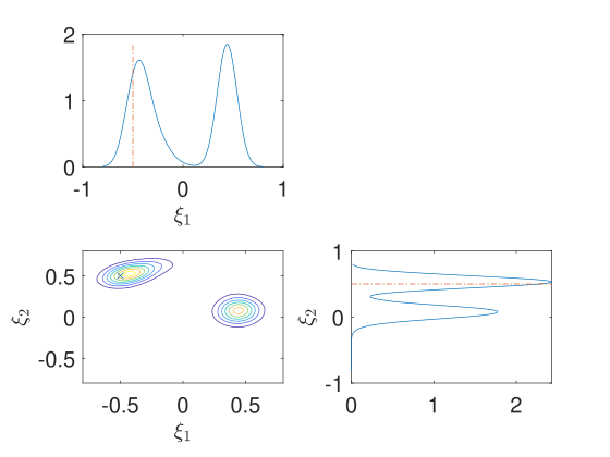
The field $u(\bm{x},t)$ is the concentration of the contaminant, and $\bm{\xi}$ represents the location of the contaminant. In this example, the location of source $\bm{\xi}$ is unknown and is considered as the inference parameter of interest. We set the prior as the uniform distribution: $\bm{\xi}\sim\mathcal{U}([-1,1]^{2})$. The truth is set to as $\bm{\xi}=[0.5,0.5]$. The observational data $\bm{d}_{obs}$ is collected at locations $(-0.4,-0.4)$ and $(0,0.4)$ at $t=0.04$. We assume that a zero mean Gaussian random noise with $5\%$ observed value covariance is considered in these observations. We use finite difference method to solve the forward model (13) with uniform meth $\Delta x=0.025$ and $\Delta t=1.25\times 10^{-4}$. The analytical form of the posterior distribution is not available, therefore we draw $5\times 10^{4}$ samples using the DREAM as the truth posterior distribution. The estimation posterior obtained by DREAM for this example is shown in Figure 1, we can see that the posterior distribution is multi-modal due to the lack of observations. One mode in the posterior distribution corresponds to the true solution, while the other mode is unknown.

Figure 1: The joint posterior distribution and the marginal probability distribution generated by DREAM (Example 1).

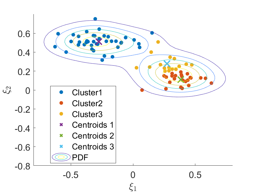
To begin with, we use the ILUES (see Algorithm 2) to generate the initial archive $\bm{Z}=\{(\bm{\xi}_{j}^{t},\bm{\tilde{\pi}}(\bm{\xi}_{j}^{t}|\bm{d}_{obs}))\}_{j=1,\ldots,N_{e},t=1,\ldots,t_{0}}$, where the forward model is defined in (13), the ensemble of size $N_{e}=80$, the initial iteration $t_{0}=1$, and the prior distribution is uniform. With the ensemble samples, we use kernel density estimation (Matlab package kde is used) to obtain the approximated PDF of $\hat{p}_{0}(\bm{\xi})$. Figure 2 (a) shows the generated samples and its corresponding estimated PDF. Compared with the true posterior (see Figure 1), we can see that with only one iteration, the ILUES is able to capture the area of high posterior distribution and can provide a good initial guess for $p_{0}(\bm{\xi})$. Next, we use the K-means method [46] to cluster the ensemble data points, Figure2(d) shows the clustering result, dots with different colors represent different clusters, the asterisks represents the mean of each cluster, and the contour is the estimated PDF from ensemble data points. The kernel function in the GP regression is set to be the squared exponential kernel function and the hyperparameters of the GP is automatically optimized via gradient descent method.

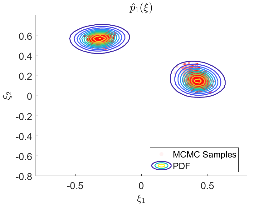
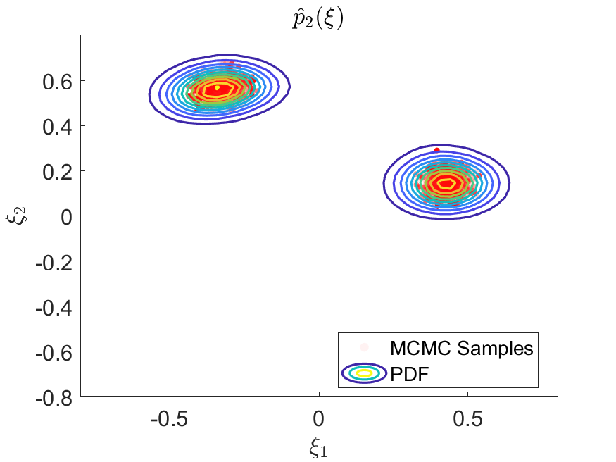
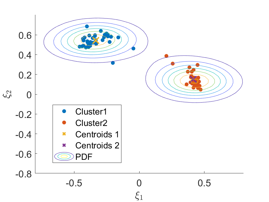
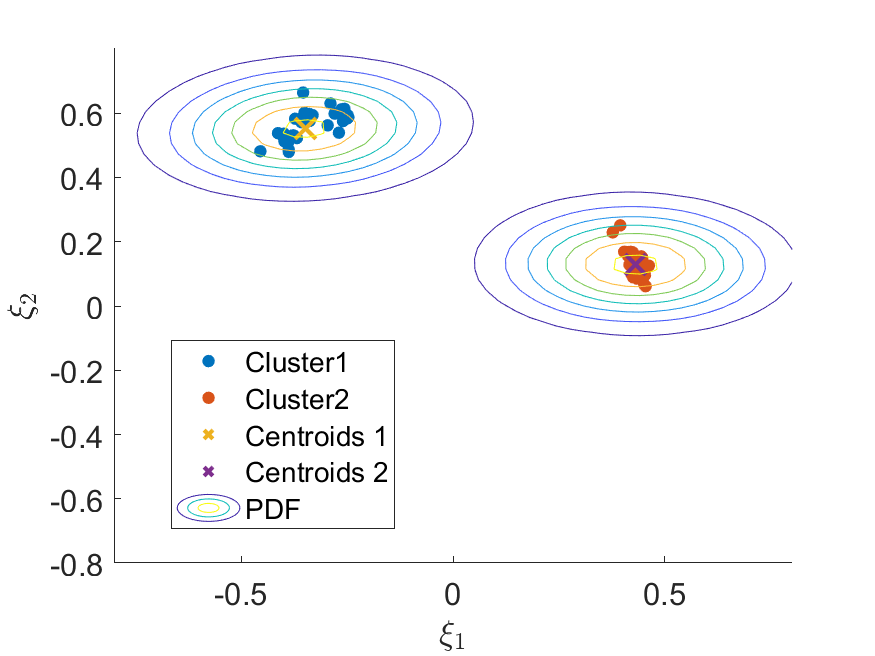
In this example, the length of MCMC is set to as $1\times 10^{4}$, and the burn-in rate is 20%. The adaptive sampling process is shown in Figure 2(a) to 2(c) , the training data points in the first iteration (see 2(a) ) are sampled from the ILUES with 1 iteration, Figure 2(b) and (c) show the estimated PDF $\hat{p}_{1}(\bm{\xi})$ and $\hat{p}_{2}(\bm{\xi})$ generated from the MCMC samples. The acceptance rates are 48.06% and 48.60% respectively, which is within the ideal range. The KL divergence from $\hat{p}_{0}(\bm{\xi})$ and $\hat{p}_{1}(\bm{\xi})$ is 0.7232, while the KL divergence from $\hat{p}_{1}(\bm{\xi})$ and $\hat{p}_{2}(\bm{\xi})$ is 0.0422, which indicates the convergence of the algorithm is soon achieved. In Figure2 (e) and (f), we present the ensemble samples with clustering information, and the contour denotes the estimated PDF from the ensemble samples at iteration $t=1$ and $t=2$. Compared with Figure2 (b) and (c), we can see that ILUES has the ability to generate samples concentrating in regions of high posterior distribution, but when the ensemble size is small, the obtained PDF is not reliable.

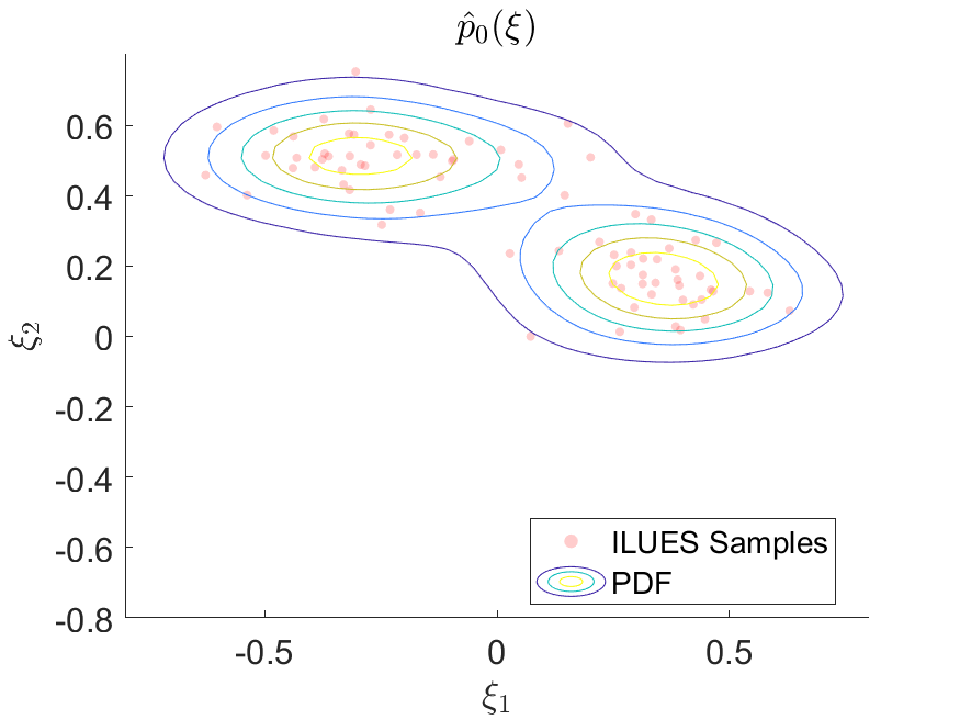
(a) Samples and the estimated PDF $\hat{p}_{0}(\bm{\xi})$. (b) The estimated PDF $\hat{p}_{1}(\bm{\xi})$ (c) The estimated PDF $\hat{p}_{2}(\bm{\xi})$ (d) The ensemble samples at iteration $t=0$. (e) The ensemble samples at iteration $t=1$. (f) The ensemble samples at iteration $t=2$.

Figure 2: Top row: The approximated posterior distributions obtained at iteration $t=0,1$ and $2$. In (a), the blue dots are ILUES ensemble points. While in (b) and (c), the samples are generated from MCMC.
Bottom row: The ensemble samples at iteration $t=0,1$ and $2$. Dots with different colors denote different clusters, the X marks denote the centroids of each cluster, and the contour denotes the estimated PDF based on the ensemble points.

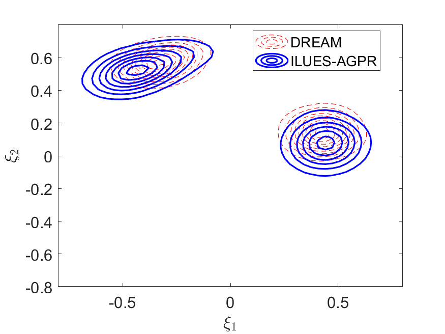
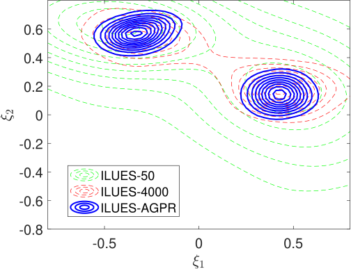
We compare the obtained posterior PDFs obtained form ILUES-AGPR, DREAM and ILUES with different ensemble sizes (see Figure 3). In Figure 3(a), we compare the posterior PDFs obtained by DREAM and our method, it can be seen that our method can capture the multi-modal posterior distribution very accurately. In Figure 3(b), we present the results obtained by ILUES, the iteration time is set to as 1, and we consider two different ensemble sizes $N_{e}=50$ and $4000$, we can see that ILUES both fail to capture the multimodality in the posterior distribution.

(a) (b)

Figure 3: Comparison among the posterior PDFs obtained by DREAM, ILUES-AGPR and ILUES with different ensemble sizes. (a) Comparison between the estimated PDFs obtained by DREAM and ILUES-AGPR. (b) Comparison among the estimated PDFs obtained by ILUES-AGPR and ILUES with different ensemble size. (ILUES-50 and ILUES-4000 denote the ILUES with $N_{e}=50$ and $4000$ respectively)

The sample Mean and Mean Square Error (MSE) of ILUES-AGPR, DREAM, ILUES with different size of ensemble as shown in Table 1. Given posterior samples $\{\bm{\xi}_{j}\}_{j=1}^{N_{sample}}$, the sample mean is computed by $\overline{\bm{\xi}}=\frac{1}{N_{sample}}\sum_{j=1}^{N_{sample}}\bm{\xi}_{j}$ and the MSE is computed by $\text{MSE}=\frac{1}{N_{sample}}\sum_{j=1}^{N_{sample}}(\bm{\xi}_{j}-\overline{\bm{\xi}})^{2}$. It can be seen that our method yields similar sample mean and MSE values as those obtained by DREAM. While ILUES with $N_{e}=50$ results in small MSE value, we can see that limited ensemble samples will cause the samples to collapse into a very small region. Increasing the ensemble sample siz $N_{e}$ will allow the MSE approach the results of the DREAM algorithm.

Table 1: Comparison of parameter results in Example 1

	Sample mean		MSE
model parameter	$\xi_{1}$	$\xi_{2}$	$\xi_{1}$	$\xi_{2}$
ILUES-AGPR	-0.085	0.230	0.0051	0.0031
DREAM	-0.049	0.275	0.0061	0.0070
ILUES($N_{e}=50$)	0.157	0.217	0.0004	0.0009
ILUES($N_{e}=500$)	0.0653	0.286	0.0011	0.0014

5.2 Example 2: contamination source location and strength identification

In this subsection, we consider a Poisson equation with mixed boundary conditions:

$$-\nabla\cdot(a(\bm{x})\nabla u(\bm{x}))=f(\bm{x}),\qquad\bm{x}\in D=[0,1]^{2},$$ (14a)

$$u(0,y)=0,\quad u(1,y)=0,$$ (14b)

and the other two boundaries are no flow boundary conditions, $a(\bm{x})$ is the permeability field and we assume the field is uniform, i.e., $a(\bm{x})=0.2$. The source term has the following form

$$f(\bm{x})=\frac{|s|}{2\pi h^{2}}\exp\left(-\frac{\|\bm{x}-\bm{\xi}\|^{2}}{2h^{2}}\right)\,,$$ (15)

where $\bm{\xi}$ is the location of the source, $h$ and $s$ are the width and strength of source, respectively. Here we suppose that the source width $h$ is known and equal to 0.05, both the strength $s$ and the source location $\bm{\xi}$ are the parameter of interest and unknown, therefore, the unknown parameter is denoted as $\theta\mathrel{\mathop{\mathchar 58\relax}}=[\xi_{1},\xi_{2},s]$.

Sensors that measure local concentration values are distributed on the uniform $3\times 3$ grid covering the domain $[0.2,0.8]\times[0.2,0.8]$, in this example, the simulated data $\bm{d}$ obtained by solving the forward model (14) on a uniform $32\times 32$ grid with a finite element solver [47]. The truth is set to as $\bm{\xi}=(0.6,0.6)$ and $s=1$. The measurement noises are set to independent and identically distributed Gaussian distributions with mean zero, and the standard deviation is set to 1% of the mean observed value. We assume the prior of $s$ is uniform $\mathcal{U}(-2,2)$ and the prior of source location $\bm{\xi}$ is uniform in the domain $D$.

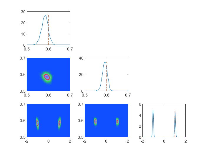
The source function (15) is symmetrical with respect to $s$, therefore, the posterior of $s$ is bimodal with modes located around 1 and -1. In contrast, the marginal distribution of the source location $\bm{\xi}$ is unimodal. We draw $5\times 10^{4}$ samples using DREAM as the truth posterior distribution (see Figure 4).

Figure 4: The joint probability density and each component marginal probability estimated by DREAM (Example 2).

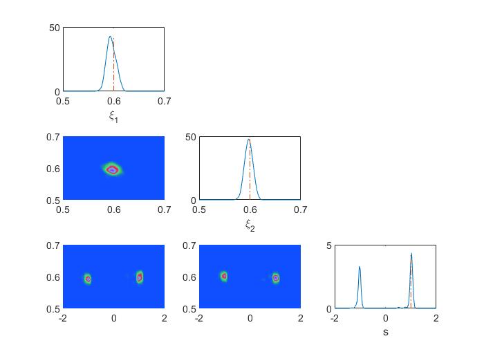
For ILUES step, we simulate $N_{e}=100$ forward model each iteration, the initial iteration $t_{0}=2$ and the algorithm iterate $N^{\max}=4$. The marginal posterior density functions of $\theta$ and the contours of the 2-dimensional marginal PDF are show plotted in Figure 5. It is obvious that the marginal posterior distribution of $s$ is bimodal, where the modes ate located at 2 and -2, and the marginal posterior distribution of source location $\bm{\xi}$ is unimodal. We can see the our method can accurately capture the multimodal posterior distribution.

Figure 5: The joint probability density and each component marginal probability estimated by ILUES-AGPR (Example 2).

6 Conclusion

Solving Bayesian inverse problems is a significant research direction in computational science. In this paper, we introduce a novel framework that efficiently generates samples from multimodal posterior distributions. The unnormalized posterior density is first expressed as a product of an auxiliary density and an exponential GP surrogate. Starting from the initial density, the auxiliary density iteratively converges to the posterior distribution. To enhance the efficiency of the GP model, we leverage the power of ILUES to generate high-quality samples. Additionally, MCMC with a GM proposal is employed to draw samples during the iterations. Numerical results demonstrate the overall efficiency of the proposed ILUES-AGPR algorithm.

References

- [1] A. Tarantola, Inverse problem theory and methods for model parameter estimation, Society for Industrial and Applied Mathematics, 2005.
- [2] J. K. Kruschke, Bayesian data analysis, Wiley Interdisciplinary Reviews: Cognitive Science 1 (5) (2010) 658–676.
- [3] H. Abarbanel, Predicting the future: completing models of observed complex systems, Springer, 2013.
- [4] M. Asch, M. Bocquet, M. Nodet, Data assimilation: methods, algorithms, and applications, SIAM, 2016.
- [5] F. Rizzi, M. Salloum, Y. Marzouk, R.-G. Xu, M. Falk, T. Weihs, G. Fritz, O. M. Knio, Bayesian inference of atomic diffusivity in a binary Ni/Al system based on molecular dynamics, Multiscale Modeling Simulation 9 (1) (2011) 486–512.
- [6] J. Kaipio, E. Somersalo, Statistical and computational inverse problems, Vol. 160, Springer Science & Business Media, 2005.
- [7] D. Luengo, L. Martino, Fully adaptive gaussian mixture metropolis-hastings algorithm, in: 2013 IEEE International Conference on Acoustics, Speech and Signal Processing, IEEE, 2013, pp. 6148–6152.
- [8] C. Andrieu, N. De Freitas, A. Doucet, M. I. Jordan, An introduction to MCMC for machine learning, Machine learning 50 (2003) 5–43.
- [9] T. Cui, K. J. Law, Y. M. Marzouk, Dimension-independent likelihood-informed MCMC, Journal of Computational Physics 304 (2016) 109–137.
- [10] J. Latz, J. P. Madrigal-Cianci, F. Nobile, R. Tempone, Generalized parallel tempering on Bayesian inverse problems, Statistics and Computing 31 (5) (2021) 67.
- [11] D. J. Earl, M. W. Deem, Parallel tempering: Theory, applications, and new perspectives, Physical Chemistry Chemical Physics 7 (23) (2005) 3910–3916.
- [12] G. Lin, Y. Wang, Z. Zhang, Multi-variance replica exchange SGMCMC for inverse and forward problems via Bayesian PINN, Journal of Computational Physics 460 (2022) 111173.
- [13] M. K. Łącki, B. Miasojedow, State-dependent swap strategies and automatic reduction of number of temperatures in adaptive parallel tempering algorithm, Statistics and Computing 26 (5) (2016) 951–964.
- [14] J. A. Vrugt, C. Ter Braak, C. Diks, B. A. Robinson, J. M. Hyman, D. Higdon, Accelerating markov chain monte carlo simulation by differential evolution with self-adaptive randomized subspace sampling, International Journal of Nonlinear Sciences and Numerical Simulation 10 (3) (2009) 273–290.
- [15] J. A. Vrugt, C. J. Ter Braak, M. P. Clark, J. M. Hyman, B. A. Robinson, Treatment of input uncertainty in hydrologic modeling: Doing hydrology backward with Markov chain Monte Carlo simulation, Water Resources Research 44 (12) (2008) W00B09.
- [16] J. Zhang, J. A. Vrugt, X. Shi, G. Lin, L. Wu, L. Zeng, Improving simulation efficiency of MCMC for inverse modeling of hydrologic systems with a kalman-inspired proposal distribution, Water Resources Research 56 (3) (2020) e2019WR025474.
- [17] I. Bilionis, N. Zabaras, B. A. Konomi, G. Lin, Multi-output separable gaussian process: Towards an efficient, fully bayesian paradigm for uncertainty quantification, Journal of Computational Physics 241 (2013) 212–239.
- [18] M. Seeger, Gaussian processes for machine learning, International Journal of Neural Systems 14 (02) (2004) 69–106.
- [19] H. Wang, J. Li, Adaptive Gaussian process approximation for Bayesian inference with expensive likelihood functions, Neural Computation 30 (11) (2018) 3072–3094.
- [20] Z. Xu, Q. Liao, Gaussian process based expected information gain computation for Bayesian optimal design, Entropy 22 (2) (2020) 258.
- [21] Y. M. Marzouk, H. N. Najm, L. A. Rahn, Stochastic spectral methods for efficient Bayesian solution of inverse problems, Journal of Computational Physics 224 (2) (2007) 560–586.
- [22] J. Li, Y. M. Marzouk, Adaptive construction of surrogates for the Bayesian solution of inverse problems, SIAM Journal on Scientific Computing 36 (3) (2014) A1163–A1186.
- [23] J. Zhang, Q. Zheng, D. Chen, L. Wu, L. Zeng, Surrogate-based Bayesian inverse modeling of the hydrological system: An adaptive approach considering surrogate approximation error, Water Resources Research 56 (1) (2020) e2019WR025721.
- [24] K. Li, K. Tang, J. Li, T. Wu, Q. Liao, A hierarchical neural hybrid method for failure probability estimation, IEEE Access 7 (2019) 112087–112096.
- [25] Y. Xia, N. Zabaras, Bayesian multiscale deep generative model for the solution of high-dimensional inverse problems, Journal of Computational Physics 455 (2022) 111008.
- [26] Y. Zhu, N. Zabaras, Bayesian deep convolutional encoder–decoder networks for surrogate modeling and uncertainty quantification, Journal of Computational Physics 366 (2018) 415–447.
- [27] A. D. Davis, Y. Marzouk, A. Smith, N. Pillai, Rate-optimal refinement strategies for local approximation MCMC, Statistics and Computing 32 (4) (2022) 1–23.
- [28] P. R. Conrad, Y. M. Marzouk, N. S. Pillai, A. Smith, Accelerating asymptotically exact MCMC for computationally intensive models via local approximations, Journal of the American Statistical Association 111 (516) (2016) 1591–1607.
- [29] P. R. Conrad, A. D. Davis, Y. M. Marzouk, N. S. Pillai, A. Smith, Parallel local approximation MCMC for expensive models, SIAM/ASA Journal on Uncertainty Quantification 6 (1) (2018) 339–373.
- [30] J. Sacks, W. J. Welch, T. J. Mitchell, H. P. Wynn, Design and analysis of computer experiments, Statistical Science 4 (4) (1989) 409–423.
- [31] D. J. MacKay, Information-based objective functions for active data selection, Neural Computation 4 (4) (1992) 590–604.
- [32] E. Cleary, A. Garbuno-Inigo, S. Lan, T. Schneider, A. M. Stuart, Calibrate, emulate, sample, Journal of Computational Physics 424 (2021) 109716.
- [33] D. J. Albers, P.-A. Blancquart, M. E. Levine, E. E. Seylabi, A. Stuart, Ensemble kalman methods with constraints, Inverse Problems 35 (9) (2019) 095007.
- [34] P. J. Van Leeuwen, G. Evensen, Data assimilation and inverse methods in terms of a probabilistic formulation, Monthly weather review 124 (12) (1996) 2898–2913.
- [35] J.-A. Skjervheim, G. Evensen, J. Hove, J. G. Vabø, An ensemble smoother for assisted history matching, in: SPE Reservoir Simulation Symposium, The Woodlands, Texas, USA, OnePetro, 2011. doi:doi.org/10.2118/141929-MS.
- [36] A. A. Emerick, A. C. Reynolds, Ensemble smoother with multiple data assimilation, Computers Geosciences 55 (2013) 3–15.
- [37] J. Zhang, G. Lin, W. Li, L. Wu, L. Zeng, An iterative local updating ensemble smoother for estimation and uncertainty assessment of hydrologic model parameters with multimodal distributions, Water Resources Research 54 (3) (2018) 1716–1733.
- [38] C. E. Rasmussen, H. Nickisch, Gaussian processes for machine learning (GPML) toolbox, The Journal of Machine Learning Research 11 (2010) 3011–3015.
- [39] R. A. Horn, C. R. Johnson, Topics in matrix analysis, Cambridge University Press, 1991.
- [40] C. Robert, G. Casella, Monte Carlo statistical methods, Springer Science & Business Media, 2013.
- [41] N. Metropolis, A. W. Rosenbluth, M. N. Rosenbluth, A. H. Teller, E. Teller, Equation of state calculations by fast computing machines, The journal of chemical physics 21 (6) (1953) 1087–1092.
- [42] W. K. Hastings, Monte Carlo sampling methods using Markov chains and their applications, Biometrika 57 (1) (1970) 97 – 109.
- [43] H. Haario, E. Saksman, J. Tamminen, An adaptive Metropolis algorithm, Bernoulli 7 (2) (2001) 223–242.
- [44] C. Andrieu, J. Thoms, A tutorial on adaptive mcmc, Statistics and computing 18 (2008) 343–373.
- [45] T. M. Kodinariya, P. R. Makwana, Review on determining number of cluster in K-means clustering, International Journal 1 (6) (2013) 90–95.
-
[46]
S. D. Landtsheer,
kmeans_opt,
MATLAB Central File Exchange. Retrieved August 15, 2024. (2024).
URL https://www.mathworks.com/matlabcentral/fileexchange/65823-kmeans_opt - [47] H. Elman, D. Silvester, A. Wathen, Finite Elements and Fast Iterative Solvers: with Applications in Incompressible Fluid Dynamics, Oxford University Press (UK), 2014.