Bounded-confidence opinion models with random-time interactions

Abstract

In models of opinion dynamics, the opinions of individual agents evolve with time. One type of opinion model is a bounded-confidence model (BCM), in which opinions take continuous values and interacting agents compromise their opinions with each other if those opinions are sufficiently similar. In studies of BCMs, it is typically assumed that interactions between agents occur at deterministic times. This assumption neglects an inherent element of randomness in social systems. In this paper, we study BCMs on networks and allow agents to interact at random times. To incorporate random-time interactions, we use renewal processes to determine social interactions, which can follow arbitrary waiting-time distributions (WTDs). We establish connections between these random-time-interaction BCMs and deterministic-time-interaction BCMs. We find that BCMs with Markovian WTDs have consistent statistical properties on different networks but that the statistical properties of BCMs with non-Markovian WTDs depend on network structure.

I Introduction

On social-media platforms, individuals engage in regular and frequent exchanges of opinions, and people’s views and how they change play a pivotal role in shaping societal discourse [1]. The study of opinion dynamics — which involves the intersection of the social and behavioral sciences, mathematics, complex systems, and other areas — has emerged as a vibrant research area that aims to determine the mechanisms that govern the formation, evolution, and dissemination of opinions in human (and animal) societies [2, 3, 4, 5, 6]. At its core, the study of opinion dynamics concerns how individuals’ beliefs, attitudes, and perceptions evolve with time through agreement, compromise, persuasion, imitation, and conflict. Understanding such dynamics is crucial to comprehend the emergence of consensus, polarization, and the resilience of diverse opinions in societies, especially in the modern ecosystem of increasingly interconnected and digital communication environments [7, 8, 9].

Researchers have studied many types of opinion models [2]. In opinion models, agents adjust their opinions based on their interactions with other agents. The opinions can update either in discrete time or in continuous time. In opinion models with discrete-time updates, time progresses through a sequence of discrete steps. Examples of models with discrete time include voter models [10], DeGroot consensus models [11], and bounded-confidence models (BCMs) [12, 13]. Opinion models with discrete-time updates are straightforward to implement for numerical computations, and one can readily incorporate various features (such as parameter adaptivity [14]) into such models. In opinion models with continuous-time interactions and hence continuous-time updates, agents continuously adjust their opinions at rates that are influenced by factors such as whether they have friendly or hostile relationships with neighbors [15] and the difference between their opinions and the opinions of their neighbors [16, 17]. Another prominent type of model with continuous-time interactions is density-based opinion models [18], which consider the collective evolution of opinions in a large population and often are described by integro-differential equations.

Several researchers have highlighted the need to incorporate stochasticity into opinion models to accurately capture the probabilistic nature of human interactions [19, 20]. One can incorporate randomness in the structure of social and communication ties between agents by using random networks, such as configuration models, stochastic block models (SBMs), and their generalizations [21]. Additionally, one can use tie-decay networks [22] (which distinguish between random communication processes and underlying social ties) and activity-driven networks [23] (which also incorporate randomness in the interactions between agents) to incorporate randomness in communication. One can also incorporate probabilistic components into the decision-making process of agents during opinion updates [24, 25, 12, 26]. For instance, the classical voter model entails the random selection of an agent and allows this agent to adopt the state of a random neighbor [25]. Similarly, in the Deffuant–Weisbuch (DW) BCM [12], one randomly chooses a pair of agents at each discrete time and then updates their opinions if their opinions are sufficiently similar. Some models also incorporate probabilistic switching between multiple opinion-update rules, such as exogenous and endogenous updates [26].

Temporal stochasticity is another form of stochasticity that is relevant to opinion models but is often overlooked. Existing opinion models typically treat time as deterministic and neglect the temporal stochasticity that is inherent in social interactions. In the present paper, we model social interactions using renewal processes [27], which consist of a sequence of random events. The time between consecutive events follows a desired waiting-time distribution (WTD). With this formulation, we are able to study non-Markovian dynamical processes, which arise in many places in human dynamics, including financial markets [28], the spread of infections diseases [29], e-mail traffic [30], and opinion dynamics [31]. We frame our discussion in the context of BCMs [32, 33]. We propose two approaches to integrate temporal stochasticity into BCMs, and we investigate the effects of stochasticity on the convergence of opinions, the formation of opinion clusters, and the expected dynamics of the opinions. We establish connections between our models and classical BCMs, and we provide an approximate approach to calculate the expected dynamics of non-Markovian opinion dynamics from discrete-time BCMs.

Our paper proceeds as follows. In Section II, we discuss single-process BCMs, in which a single renewal process dictates all agents’ interaction times. We explore these models with both synchronous and asynchronous update rules by examining properties such as expected dynamics, convergence, and other aspects for different WTDs. In Section III, we discuss multiple-process BCMs, where independent renewal processes govern the interaction times between each pair of agents. We derive the expected dynamics for Markovian BCMs in this framework, and we use a Gillespie algorithm to efficiently simulate event times for non-Markovian BCMs. In Section IV, we conclude and discuss future directions. Our code is available at https://bitbucket.org/chuwq/bounded_confidence_models_with/src/main/.

II Single-process BCMs

II.1 Random-time interactions

Consider an unweighted and directed network $G=(V,E)$, where $V=\{1,2,\ldots,N\}$ is the set of nodes (i.e., agents) and $E=\{e_{ij}\}$ is the set of edges (i.e., social ties between agents). The edge $e_{ij}$ is directed from agent $j$ to agent $i$. Each agent $i$ has a scalar continuous-valued opinion $x_{i}(t)$. When $e_{ij}=1$, agent $j$ can potentially influence agent $i$’s opinion. In a classical BCM [33, 12, 13], time is deterministic and takes discrete values, with social interactions and opinion updates occurring at intervals of and $\Delta t$. For convenience, researchers often set $\Delta t=1$.

Let $R(t)$ be a renewal process, which is a stochastic process that models a sequence of events that occur randomly in time [27]. Let $\mathcal{T}=\left\{t_{0},t_{1},t_{2},\ldots\right\}$ be the sequence of event times from the renewal process $R(t)$. We set $t_{0}=0$ as the starting time of the renewal process. The time increments (i.e., “interevent times”) $t_{k+1}-t_{k}$ are independent and identically distributed (IID) random variables that satisfy a waiting-time distribution (WTD) $\psi(t)$. In this section, we suppose that a single renewal process determines the interaction times.

II.2 Synchronous and asynchronous opinion-update rules

The Hegselmann–Krause (HK) model [13] is a discrete-time BCM with a synchronous opinion-update rule. That is, all agents update their opinions simultaneously. Let

$$\mathcal{N}_{i}(t)=\{i\}\cup\left\{j:\leavevmode\nobreak\ e_{ij}\in E\,\,\text{\leavevmode\nobreak\ and\leavevmode\nobreak\ }\,\,|x_{i}(t)-x_{j}(t)|<c\right\}$$ (1)

be the set of neighbors of agent $i$ (including itself) with which it interacts at time $t$. The parameter $c$ is the confidence bound. In each time step, the opinion of each agent $i$ updates through the rule

$$x_{i}(t+{\triangle t})=\frac{\sum_{j\in\mathcal{N}_{i}(t)}x_{j}(t)}{|\mathcal{N}_{i}(t)|}\,,\quad t=0,\,{\triangle t},\,2{\triangle t},\,\ldots\,\,.$$ (2)

We extend the HK BCM to a continuous-time model with interactions at random times. Agents update their opinions synchronously when an event occurs in the renewal process $R(t)$. The opinion-update rule is thus

$$x_{i}(t)=\frac{\sum_{j\in\mathcal{N}_{i}(t_{-})}x_{j}(t_{-})}{|\mathcal{N}_{i}(t_{-})|}\,,\quad t\in\mathcal{T}=\{t_{1},t_{2},\ldots\}\,,$$ (3)

where $t_{-}$ denotes the time that is instantaneously before time $t$. Therefore, $x_{j}(t_{-})$ is the opinion of agent $j$ right before it updates its opinion at time $t$. Unless an event occurs at time $t\in\mathcal{T}$, the opinions of all agents stay the same. We refer to the BCM with the opinion-update rule (3) as a single-process BCM with synchronous updates. When the WTD $\psi$ is the Dirac delta distribution (i.e., $\psi(t)=\delta(t-{\triangle t})$), the update rule (3) reduces to the update rule (2) in the classical HK BCM [13].

Deffuant et al. [12] introduced a discrete-time BCM with an asynchronous opinion-update rule. At each discrete time step, one selects a pair of agents uniformly at random and updates their opinions to the mean of their opinions (or, more generally, to opinions that are closer to the mean) if their opinion difference is smaller than a confidence bound $c$. This model, which is known as the Deffuant–Weisbuch (DW) BCM, was proposed in the context of undirected graphs. We extend the DW BCM to a directed DW BCM. In this directed DW model, at time step $t$, one selects an edge $e_{ij}$ uniformly at random and updates the opinion of agent $i$ with the rule

$$x_{i}(t+{\triangle t})=\begin{cases}\frac{1}{2}\left[x_{j}(t)+x_{i}(t)\right]&\text{if}\,\,|x_{i}(t)-x_{j}(t)|<c\\ x_{i}(t)&\text{otherwise}\,.\end{cases}$$ (4)

The opinions of all other agents stay the same. The time $t$ takes values from the set $\left\{0,\,{\triangle t},\,2{\triangle t},\,\ldots\right\}$.

We generalize the directed DW BCM (4) to a continuous-time model by allowing interactions at random times. At time $t\in\mathcal{T}$, where $\mathcal{T}$ is the set of event times of a renewal process, we select an edge $e_{ij}$ uniformly at random and update the opinions of agent $i$ with the rule

$$x_{i}(t)=\begin{cases}\frac{1}{2}\left[x_{j}(t_{-})+x_{i}(t_{-})\right]&\text{if}\,\,|x_{i}(t_{-})-x_{j}(t_{-})|<c\\ x_{i}(t_{-})&\text{otherwise}\,.\end{cases}$$ (5)

The opinions of all other agents stay the same. Additionally, unless an event occurs at time $t\in\mathcal{T}$, the opinions of all agents stay the same. We refer to the BCM with the opinion-update rule (5) as a single-process BCM with asynchronous updates. When the WTD $\psi$ is the Dirac delta distribution (i.e., $\psi(t)=\delta(t-{\triangle t})$), the update rule (5) is the same as in the directed DW BCM (4).

In the random-time BCMs with synchronous (3) and asynchronous (5) update rules, the agent opinions converge almost surely to isolated opinion clusters (i.e., maximal sets of agents with the same opinion value) that differ by at least the confidence bound $c$. This is a direct consequence of Lorenz’s stability theorem [36].

II.3 Comparisons between the update rules (3) and (5)

In Figure 1(a), we show the event times that are generated by renewal processes with the WTDs

$$\psi_{\text{uniform}}(t) =\delta(t-\mu)\,,$$ (6a)

$$\psi_{\text{exponential}}(t) =\frac{1}{\mu}\exp(-t/\mu)\,,$$ (6b)

$$\psi_{\text{gamma}}(t) =\frac{4t}{\mu^{2}}\exp(-2t/\mu)\,,$$ (6c)

$$\psi_{\text{uniform}}(t) =\mathbbm{1}_{[0,2\mu]}(t)\,,$$ (6d)

where $\mathbbm{1}_{S}$ denotes the indicator function on the set $S$. All WTDs have the same mean value $\mu$. We simulate single-process BCMs with synchronous (3) and asynchronous (5) updates on a complete graph with $50$ agents and show the resulting opinions in Figure 1(b,c).

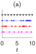
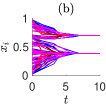
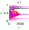
Figure 1: (a) Event times of renewal processes when the WTDs are the Dirac delta, exponential, gamma, and uniform distributions in (6) with mean $\mu=1$. (b,c) Time-dependent opinions of a single-process BCM with (b) synchronous opinion updates (3) and (c) asynchronous opinion updates (5). The confidence bound is $c=0.2$. All simulations in (b) and (c) have the same initial opinions, which we draw randomly from a uniform distribution on $[0,1]$.

In the single-process BCM with synchronous updates (3) with a given set of initial opinions, the node opinions always converge to the same steady state for all of the WTDs. This is an expected result because the opinion updates in (3) are deterministic once one determines the interaction times. The random interaction times only affect when the opinion updates occur; the updates themselves are the same. By contrast, simulations with asynchronous opinion updates converge to diverse steady states due to the randomness in edge selection. Nevertheless, it is noteworthy that the expected steady-state opinions of the asynchronous single-process BCM (5) are the same for the different WTDs. In Section II.4, we give a detailed explanation of why the expected steady-state opinions do not depend on the WTD. Additionally, because the asynchronous model updates the opinions of one pair of agents at a time, it has significantly longer convergence times than the synchronous model. For the same reason, the classical DW BCM has much longer convergence times than the classical HK BCM [37, 12, 13].

II.4 Exact and approximate dynamics of the expected opinions

Let ${\bm{x}}(t)=(x_{1}(t),\ldots,x_{N}(t))\in\mathbb{R}^{N}$ be the time-dependent opinion vector of the single-process BCM (3) or (5). The randomness in $\bm{x}(t)$ arises from the interaction times, the selection of edges in the asynchronous-update model (5), and potentially random initial opinions. These three sources of randomness are independent of each other. In the rest of this section, we fix the initial opinion vector $\bm{x}_{0}$ and investigate how the other two sources of randomness influence the dynamics of the expected opinions. We also examine how the WTDs influence the dynamics of the expected opinions in single-process BCMs with the synchronous update rule (3) and the asynchronous update rule (5).

Let $u_{k}(t)$ denote the probability that the renewal process $R(t)$ has $k$ events in the time interval $[0,t]$. The probability $u_{k}(t)$ satisfies

$$u_{0}(t) =1-\int_{0}^{t}\psi(\tau)\mathrm{d}\tau\,,$$ (7)

$$u_{k+1}(t) =\int_{0}^{t}\psi(\tau)u_{k}(t-\tau)\mathrm{d}\tau\,,\leavevmode\nobreak\ \leavevmode\nobreak\ k\geq 0\,,$$

where $\psi$ is the WTD. For any function $f:\mathbb{R}^{N}\longrightarrow\mathbb{R}$, let $\mathbb{E}[f]$ denote the expectation of $f(\bm{x})$. We thus write

$$\mathbb{E}[f](t)=\mathbb{E}[f({\bm{x}}(t))]\,.$$ (8)

We take this expectation with respect to all randomness except for the initial opinions. Let $\bm{x}[k]$ denote the opinion vector after $k$ updates, and let $\mathbb{E}_{k}[f]$ be the expected value of $f(\bm{x}[k])$. The event times are independent of opinion updates, so

$$\mathbb{E}[f](t)=\sum_{k=0}^{\infty}\mathbb{E}_{k}[f]u_{k}(t)\,.$$ (9)

The probability $u_{k}(t)$ is determined solely by the WTD $\psi$; it is independent of the update rules (3) and (5). The expectation $\mathbb{E}_{k}[f]$ is independent of both the WTD $\psi$ and the renewal process; it is determined solely by the update rules (3) and (5). By using (9), we disassociate the expected opinion dynamics from the temporal stochasticity that arises from the random-time interactions. By introducing a cutoff for $k$, equation (9) yields an approximate formula to compute the expected dynamics of the BCMs with random-time interactions.

We compute the probability $u_{k}(t)$ either directly using (7) or by employing the Laplace transforms of $u_{k}(t)$ to circumvent calculating the convolution. See [31, 38] for how to derive the Laplace transforms of the probability $u_{k}(t)$. The synchronous single-process BCM has a deterministic update rule (3). Therefore, $\mathbb{E}_{k}[f]=f(x[k])$ and we obtain $\mathbb{E}_{k}[f]$ in (9) with a single simulation of the discrete-time HK BCM (2). That is, we simulate “one realization” of the discrete-time HK BCM (2). For the asynchronous single-process BCM, it is often challenging to evaluate $\mathbb{E}_{k}[f]$ due to the randomness in selecting node pairs for potential opinion updates. This randomness can yield different opinion trajectories for any WTD (even for the Dirac delta WTD). Therefore, we need to simulate multiple realizations of the discrete-time directed DW BCM (4) to approximate the expectation $\mathbb{E}_{k}[f]$.

To quantify the amount of consensus in a simulation of a single-process BCM, we calculate the order parameter

$$Q(\bm{x})=\frac{1}{|E|}\sum_{e_{ij}\in E}\mathbbm{1}_{x_{i}=x_{j}}\,.$$ (10)

When $Q=1$, all agents have the same opinion and the system is in its most ordered phase. Conversely, when $Q=1/N$ (where $N$ is the number of agents), each agent has a different opinion, and the system is in its least ordered phase. In practice, we often relax the condition $\mathbbm{1}_{x_{i}=x_{j}}$ by instead using $\mathbbm{1}_{|x_{i}-x_{j}|<\texttt{tol}}$ (where tol is a tolerance parameter) to hasten the convergence of simulations.

In Figure 2, we compute the mean of the order parameter for the synchronous single-process BCM (3) for different WTDs and approximate the expected order parameters for the same models using (9). As we increase the number of simulations, we observe that the time-dependent order parameters become smoother for the continuous WTDs (i.e., the exponential, Gamma, and uniform WTDs) and that the trajectories of the approximate expected order parameters closely match those of the mean order parameters for all WTDs.

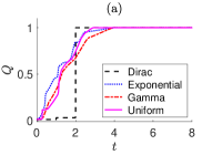
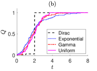
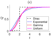
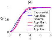
Figure 2: In (a)–(c), we show the mean of the order parameter $Q$ [see (10)] of (a) $10$, (b) $100$, and (c) $1000$ simulations of the synchronous single-process BCM (3) on a 100-node complete graph. For each simulation, we draw the initial opinions from the uniform distribution on $[0,1]$. The confidence bound is $c=0.5$, and the tolerance parameter is $\texttt{tol}=10^{-2}$. In (d), we plot the mean value of $Q$ from (c) for different WTDs and their approximations using (9). In the approximation, we use $15$ as the upper bound of $k$.

III Multiple-process BCMs

The single-process BCMs in Section II assume that a single renewal process governs when interactions between agents occur. In reality, however, people exchange opinions at various times, so one cannot expect the interactions between agents to be governed by one renewal process. Therefore, we consider multiple independent renewal processes $R_{ij}$, which determine when each agent $i$ interacts with each agent $j$. Such an interaction can potentially update the opinion of agent $i$.

III.1 Asynchronous interactions from multiple renewal processes

Let $R_{ij}$ be a renewal process that generates a sequence of event times $\mathcal{T}_{ij}=\{t_{0},t_{1},t_{2},\ldots\}$ with initial time $t_{0}=0$. We suppose that all renewal processes $R_{ij}$ are independent of each other and have the same WTD $\psi$. The renewal process $R_{ij}$ determines the interaction times from agent $j$ to agent $i$. At time $t\in\mathcal{T}_{ij}$, we update the opinion $x_{i}$ of node $i$ using the update rule

$$x_{i}(t)=\begin{cases}\frac{1}{2}\left[x_{i}(t_{-})+x_{j}(t_{-})\right]&\text{if\leavevmode\nobreak\ }\left|x_{i}(t_{-})-x_{j}(t_{-})\right|<c\\ x_{i}(t_{-})&\text{otherwise}\,.\end{cases}$$ (11)

The opinions of all other agents stay the same. If multiple events that involve the same agent $i$ occur simultaneously at time $t$, then we update its opinion $x_{i}$ to

$$x_{i}(t)=\frac{\sum_{j\in\tilde{\mathcal{N}}_{i}(t_{-})}x_{j}(t_{-})}{|\tilde{\mathcal{N}}_{i}(t_{-})|}\,,$$ (12)

where

$$\tilde{\mathcal{N}}_{i}(t)=\left\{i\right\}\cup\left\{j\in{\mathcal{N}}_{i}(t):\leavevmode\nobreak\ t\in\mathcal{T}_{ij}\right\}$$ (13)

is a restricted neighbor set (which differs from the neighbor set (1)) that includes all neighboring nodes of $i$ that (1) interact with node $i$ at time $t$ and (2) have an opinion that differs from $x_{i}$ by less than the confidence bound $c$. We refer to (11) as a multiple-process BCM. When the WTD $\psi$ is continuous, the events of two renewal processes occur simultaneously with $0$ probability, so opinion updates in (11) are asynchronous almost surely (i.e., with probability $1$). When the WTD $\psi(t)=\delta(t-{\triangle t})$ is a Dirac delta distribution, the events of different processes occur simultaneously at times $t={\triangle t},\,2{\triangle t},\,\ldots$, and we obtain the synchronous single-process BCM in Section II.2. We can extend the multiple-process BCM (11) to a heterogeneous scenario in which each renewal process $R_{ij}$ has a different WTD $\psi_{ij}$. In such a model, opinion updates can occur as a hybrid of synchronous and asynchronous updates.

III.2 Dynamics of Markovian multiple-process BCMs

We now discuss the dynamics of some Markovian multiple-process BCMs. When the WTD is a Dirac delta distribution, both the single-process BCM (3) and the multiple-process BCM (11) become discrete-time Markovian processes. In this situation, both models reduce to the classical HK BCM [13]. In the rest of this subsection, we consider continuous-time Markovian BCMs with an exponential WTD. To help highlight their dynamics, we also compare them to BCMs with the Dirac delta WTD.

When the WTD $\psi(t)$ is exponential, the renewal processes $R_{ij}$ are Poisson point processes. We write $\psi(t)=\lambda e^{-\lambda t}$, where $\lambda$ is the rate parameter of the process. The sum (i.e., “superposition”) of $|E|$ Poisson point processes is a Poisson point process $P(t)$ with rate parameter $\Lambda=\lambda|E|$. In this case, the multiple-process BCM is the same as the asynchronous single-process BCM (5) with an exponential WTD with decay rate $\Lambda$. We will show that the opinion model that is induced by the exponential WTD is Markovian, and we will relate the dynamics of the expected opinions to a continuous-time HK BCM [16].

Let $P(t)$ be the superposition of all $|E|$ Poisson point processes $R_{ij}$ (where $E$ is the set of edges of a network), and let $Z$ denote the total number of events in the time interval $[t,t+\tau)$ for $P(t)$. We have

$$Z=\begin{cases}0&\text{with probability}\quad e^{-\Lambda\tau}\\ 1&\text{with probability}\quad\Lambda\tau\,e^{-\Lambda\tau}\\ \geq 2&\text{with probability}\quad\sum_{k=2}^{\infty}\frac{(\Lambda\tau)^{k}}{k!}e^{-\Lambda\tau}\,.\end{cases}$$ (14)

When $Z=0$, no opinion update occurs in the time interval $[t,t+\tau)$, so this situation does not contribute to opinion updates. When $Z=1$, one event occurs in the time interval $[t,t+\tau)$. This event is associated with the process $R_{ij}$ with probability $1/|E|$. In this event, agent $i$ changes its opinion by

$$\triangle_{i,j}(t)=\frac{1}{2}\mathbbm{1}_{|x_{i}(t)-x_{j}(t)|<c}\left[x_{j}(t)-x_{i}(t)\right]\,.$$ (15)

Let $y_{i}(t)=\mathbb{E}[x_{i}(t)]$ be the expectation with respect to the superposition $P(t)$. The expected opinion of $y_{i}(t+\tau)$ satisfies

$$y_{i}(t+\tau) =y_{i}(t)+\!\!\sum_{{\{}j:e_{ij}\in E{\}}}\frac{\Lambda\tau}{|E|}\,e^{-\Lambda\tau}\mathbb{E}\left[\triangle_{i,j}(t)\right]+\mathcal{O}(\tau^{2})\,,$$ (16)

where $\mathcal{O}(\tau^{2})$ arises from the contribution for $Z\geq 2$. We use the relation $\Lambda=\lambda|E|$ and then take the limit $\tau\to 0$ to obtain

$$\dot{y}_{i}(t)= \frac{\lambda}{2}\sum_{{\{j:e_{ij}\in E\}}}\!\!\mathbb{E}\left\{\mathbbm{1}_{|x_{i}(t)-x_{j}(t)|<c}\left[x_{j}(t)-x_{i}(t)\right]\right\}\,,$$ (17)

where $i\in\{1,\ldots,N\}$. The system (17) is not closed. We make the bold approximation

$$\mathbb{E}\left\{\mathbbm{1}_{|x_{i}(t)-x_{j}(t)|<c}\left[x_{i}(t)-x_{j}(t)\right]\right\}$$ (18)

$$\quad\quad\approx\mathbbm{1}_{|y_{i}(t)-y_{j}(t)|<c}\left[y_{i}(t)-y_{j}(t)\right]$$

and thereby obtain

$$\dot{y}_{i}(t)=\frac{\lambda}{2}\sum_{{\{j:e_{ij}\in E\}}}\mathbbm{1}_{|y_{i}(t)-y_{j}(t)|<c}\left[y_{j}(t)-y_{i}(t)\right]\,,$$ (19)

which is a continuous-time HK BCM [16] with $\lambda=2$ and $c=1$.

The approximation (18) is a special form of $\mathbb{E}[g(r)]\approx g(\mathbb{E}[r])$; we obtain the approximation (18) when $g(r)=\mathbbm{1}_{|r|<c}r$ and $r=x_{i}-x_{j}$. For a general random variable $r$, the expectation $\mathbb{E}[g(r)]$ does not equal $g(\mathbb{E}[r])$. They are equal to each other for two special cases: (1) when $g$ is linear; and (2) when $r$ follows a Dirac delta distribution. In our numerical simulations, we observe discrepancies between (17) and (19).

The expected dynamics (17) is related to the asynchronous single-process BCM (5) when the WTD is $\psi(t)=\delta(t-{\triangle t})$ and ${\triangle t}=1/(\lambda|E|)$. This model updates opinions at discrete times $t={\triangle t},\,2{\triangle t},\,\ldots$ . We consider a piecewise-linear interpolation of the opinions $x_{i}(t)$ on each time interval $[k{\triangle t},(k+1){\triangle t})$ with the opinions at the two interval endpoints. The expected opinions satisfy

$$\dot{y}_{i}(t)=\frac{\lambda}{2}\!\sum_{{\{j:e_{ij}\in E\}}}\!\!\!\mathbb{E}\left\{\mathbbm{1}_{|{r_{ji}(k{\triangle t})}|<c}{r_{ji}(k{\triangle t})}\right\}$$ (20)

for $t\in[k{\triangle t},(k+1){\triangle t})$, where $r_{ji}(k{\triangle t})=x_{j}(k{\triangle t})-x_{i}(k{\triangle t})$. In our numerical simulations, we observe that (17) and (20) yield the same dynamics as we increase the number of realizations to evaluate the expectations.

In Figure 3, we show the mean time-dependent opinions of three Markovian models: the asynchronous single-process BCM (5) with the Dirac delta WTD $\psi(t)=\delta(t-1/(\lambda|E|))$ (which we denote by “S-Dirac”), the asynchronous single-process BCM (5) with the exponential WTD $\psi(t)=\lambda|E|\exp(-\lambda|E|t)$ (which we denote by “S-Exp”), and the multiple-process BCM (11) with the exponential WTD $\psi(t)=\lambda\exp(-\lambda t)$ (which we denote by “M-Exp”). Because each realization can have distinct opinion update times, we use a piecewise-linear interpolation for opinions at discrete update times for each realization and then compute the mean of the interpolated opinion trajectories on the entire time domain. We then compute the mean opinion dynamics by averaging the interpolated dynamics across multiple simulations of the same model.

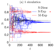
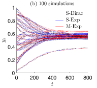
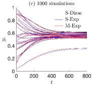
Figure 3: The mean time-dependent opinions $y_{i}(t)$ in the asynchronous single-process BCMs (5) (S-Dirac and S-Exp) and the multiple-process BCM (11) (M-Exp) of (a) 1, (b) 100, (c) 1000, and (d) 2000 simulations. All simulations have the same initial opinions, which we draw uniformly at random from $[0,1]$. We run these simulations on a 25-node Erdős–Rényi graph with edges that exist with independent probability $p=0.5$. The confidence bound is $c=0.4$.

III.3 Gillespie algorithm for non-Markovian multiple-process BCMs

It is computationally challenging to simulate a large number of processes in a multiple-process BCM (11) with $|E|$ renewal processes operating independently and concurrently. It is prohibitively complex to simulate these processes separately, organize their events chronologically, and execute opinion updates. To mitigate this computational burden, we use a Gillespie algorithm [39], which allows us to generate independent stochastic processes efficiently and statistically correctly.

The traditional Gillespie algorithm [40] is for independent Poisson processes, whose WTDs are exponential. Boguñá et al. [41] extended the Gillespie algorithm to simulate the events of multiple independent renewal processes. Their non-Markovian Gillespie algorithm draws a time increment ${\triangle t}$ for the time to the next event from the superposition of $m$ renewal processes and determines the process that produces that event with a probability that depends on the waiting time of each renewal process. This Gillespie algorithm, which we state in Algorithm 1, generates a statistically correct sequence of event times. One can terminate the algorithm after a specified number of events or when the time reaches a specified value. When all renewal processes are Poisson processes, the instantaneous rate $\lambda_{\alpha}(t)$ in (23) reduces to the constant $\lambda_{\alpha}$, which is the rate of the $\alpha$th Poisson point process. That is, in this situation, this non-Markovian Gillespie algorithm reduces to the traditional Gillespie algorithm.

Algorithm 1 Gillespie algorithm to simulate $m$ independent renewal processes

1:Initialize $t_{\alpha}=0$ for all $\alpha\in\{1,\ldots,m\}$.

2:Draw a uniform random variable $u$ from $[0,1]$ and determine the time increment ${\triangle t}$ by solving

$$\Phi\left({\triangle t}\mid\left\{t_{\alpha}\right\}\right)=\prod_{\alpha}\frac{\psi_{\alpha}(t_{\alpha}+{\triangle t})}{\Psi(t_{\alpha})}=u\,,$$ (21)

where $\psi_{\alpha}$ is the WTD of the $\alpha$th renewal process and $\Psi_{\alpha}(t)=\int_{-\infty}^{t}\psi_{\alpha}(\tau)\mathrm{d}\tau$ is the survival function.

3:Randomly select a process $\beta$ that generates the event with probability

$$\Pi_{\beta}=\frac{\lambda_{\beta}\left(t_{\beta}+\Delta t\right)}{\sum_{\alpha=1}^{m}\lambda_{\alpha}\left(t_{\alpha}+\Delta t\right)}\,,$$ (22)

where

$$\lambda_{\alpha}\left(t\right)=\frac{\psi_{\alpha}\left(t\right)}{\Psi_{\alpha}\left(t\right)}$$ (23)

is the instantaneous rate of the $\alpha$th process.

4:Set $t_{\beta}=0$ and update $t_{\alpha}$ to $t_{\alpha}+\Delta t$ for $\alpha\neq{\beta}$.

5:Repeat steps 2–4 (or terminate the algorithm if a stopping criterion is satisfied).

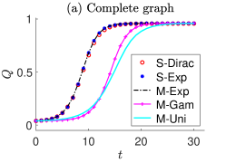
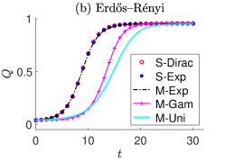
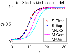
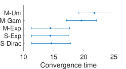
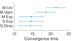
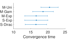
Figure 4: The (top) mean of the order parameter $Q$ (see (10)) versus time and (bottom) mean and standard deviation of the convergence time for single-process BCMs (5) with Dirac delta (S-Dirac) and exponential (S-Exp) WTDs and for multiple-process BCMs (11) with exponential (M-Exp), gamma (M-Gam), and uniform (M-Uni) WTDs. The confidence bound is $c=0.4$, and the distribution mean is $\mu=0.01$. We show results for 1000 BCM simulations on (a) a complete graph, (b) Erdős–Rényi graphs, and (c) two-community stochastic-block-model graphs. We draw the initial opinions uniformly at random from $[0,1]$ for each realization, we and generate a new random graph for each simulation in (b) and (c).

We use the non-Markovian Gillespie algorithm in Algorithm 1 to simulate the multiple-process BCM (11) on three distinct types of 50-node graphs: (1) a complete graph; (2) Erdős–Rényi random graphs in which each edge exists with independent probability $p=0.85$; and (3) stochastic-block-model graphs with two communities, intra-community probability $p_{\text{in}}=0.8$, and inter-community probability $p_{\text{out}}=0.2$. We explore how randomness, which arises through the WTDs and graphs, influences the convergence time and overall dynamics in both single-process and multiple-process BCMs. For the single-process BCMs, we use Dirac delta and exponential WTDs with mean $\mu|E|$, ensuring that all simulations have the same expected number of events during the simulation period. For the multiple-process BCMs (11), we consider exponential, gamma, and uniform WTDs with mean $\mu$. In Figure 4, we show (1) the mean order parameter $Q$ (10) of 1000 simulations for each model and (2) the mean convergence time and associated standard deviation. We generate a new random graph for each simulation.

We observe that the three Markovian models — the single-process BCM with the Dirac delta WTD, the single-process BCM with the exponential WTD, and the multiple-process BCM with exponential WTD — yield almost identical mean time-dependent order parameters $Q$. This observation aligns with the results in Figure 3, in which the mean opinions yield the same dynamics as we increase the number of simulations. However, for multiple-process BCMs with gamma and uniform WTDs, the order parameter $Q$ has distinct transient behaviors, with convergence rates that depend both on the WTDs and on the network structure. Across various networks and across different WTDs, the mean order parameter converges to the same steady state. This convergence occurs predominantly due to simulations converging to a consensus state for the confidence bound $c=0.4$. However, for the smaller confidence bound $c=0.3$, we observe distinct steady-state order parameters (see Figure 5). We also examine the convergence times of the single-process BCM (5) and the multiple-process BCM (11) with different WTDs. Based on our numerical observations, we see that both WTDs and network structure influence the convergence time, with networks primarily impacting the variance of the convergence time.

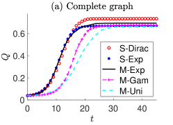
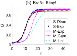
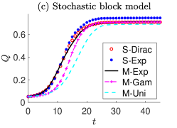
Figure 5: The mean of the order parameter $Q$ (see (10)) over 1000 simulations of single-process BCMs (5) with Dirac delta (S-Dirac) and exponential (S-Exp) WTDs and multiple-process BCMs (11) with exponential (M-Exp), gamma (M-Gam), and uniform (M-Uni) WTDs on (a) a complete graph, (b) Erdős–Rényi graphs, and (c) stochastic-block-model graphs. We repeat the same simulation process as in Figure 4 (including generating a new set of graphs), except that now the confidence bound is $c=0.3$.

IV Conclusions and discussion

We extended classical bounded-confidence models (BCMs) by incorporating stochasticity into agent interaction times. We incorporated temporal stochasticity using renewal processes and allowed social interactions to occur either synchronously or asynchronously. Using both numerical simulations and analytical arguments, we obtained insights into the dynamics of our BCMs on networks.

In single-process BCMs (3) and (5), for which a single renewal process governs the interaction times between agents, we found that waiting-time distributions (WTDs) primarily influence the transient opinion dynamics while yielding the same steady-state outcomes. For a Dirac delta distribution WTD, our single-process BCMs reduce to the classical Hegselmann–Krause BCM [13] and a directed variant of the Deffuant–Weisbuch BCM [12]. For various WTDs, we derived the expected dynamics of the single-process BCMs (3) and (5). We approximated the expected dynamics of the single-process random-time BCMs with the dynamics of deterministic-time BCMs and demonstrated numerically that this approximation is effective.

We also developed multiple-process BCMs (5), which use multiple independent renewal processes to control the interaction times between agents. Multiple-process BCMs with Dirac delta and exponential WTDs yield Markovian models that are equivalent to single-process BCMs with appropriately chosen WTDs and parameters. We derived an approximate governing equation for the expected opinions in these two Markovian models. For specific parameter values, these two models reduce to the continuous-time BCM in [16]. To simulate multiple-process BCMs with various WTDs, we employed a non-Markovian Gillespie algorithm [41]. In these numerical computations, we observed that both WTDs and network structure influence the properties of the non-Markovian models, including the order parameter (10) and convergence time.

In the present paper, we considered unweighted graphs and assumed that WTDs are homogeneous across all edges. It is worthwhile to incorporate both heterogeneous edge weights and heterogeneous WTDs. In such extensions, one can incorporate heterogeneity in a network’s edges (as opposed to the node heterogeneities in Ref. [35]) and use weighted averages in synchronous opinion updates (3) or encode heterogeneous WTDs with parameters that are linked to edge weights. Another interesting avenue is to incorporate temporal stochasticity into density-based BCMs [18, 42], which describe the collective behavior of a large population of agents and take the form of integro-differential equations. Naturally, it is also worth exploring the behavior of BCMs with random-time interactions on real social networks and with WTDs that are estimated from empirical data.

References

- Bak-Coleman et al. [2021] J. B. Bak-Coleman, M. Alfano, W. Barfuss, C. T. Bergstrom, M. A. Centeno, I. D. Couzin, J. F. Donges, M. Galesic, A. S. Gersick, J. Jacquet, A. B. Kao, R. E. Moran, P. Romanczuk, D. I. Rubenstein, K. J. Tombak, J. J. Van Bavel, and E. U. Weber, Stewardship of global collective behavior, Proceedings of the National Academy of Sciences of the United States of America 118, e2025764118 (2021).
- Noorazar et al. [2020] H. Noorazar, K. R. Vixie, A. Talebanpour, and Y. Hu, From classical to modern opinion dynamics, International Journal of Modern Physics C 31, 2050101 (2020).
- Olsson and Galesic [2024] H. Olsson and M. Galesic, Analogies for modeling belief dynamics, Trends in Cognitive Sciences (2024), available at https://doi.org/10.1016/j.tics.2024.07.001.
- Castellano et al. [2009] C. Castellano, S. Fortunato, and V. Loreto, Statistical physics of social dynamics, Reviews of Modern Physics 81, 591 (2009).
- Sen and Chakrabarti [2014] P. Sen and B. K. Chakrabarti, Sociophysics: An Introduction (Oxford University Press, Oxford, UK, 2014).
- Jusup et al. [2022] M. Jusup, P. Holme, K. Kanazawa, M. Takayasu, I. Romić, Z. Wang, S. Geček, T. Lipić, B. Podobnik, L. Wang, W. Luo, T. Klanjšček, J. Fan, S. Boccaletti, and M. Perc, Social physics, Physics Reports 948, 1 (2022).
- Amelkin et al. [2017] V. Amelkin, F. Bullo, and A. K. Singh, Polar opinion dynamics in social networks, IEEE Transactions on Automatic Control 62, 5650 (2017).
- Mathias et al. [2017] J.-D. Mathias, S. Huet, and G. Deffuant, An energy-like indicator to assess opinion resilience, Physica A: Statistical Mechanics and its Applications 473, 501 (2017).
- Grabowski [2009] A. Grabowski, Opinion formation in a social network: The role of human activity, Physica A: Statistical Mechanics and its Applications 388, 961 (2009).
- Sood and Redner [2005] V. Sood and S. Redner, Voter model on heterogeneous graphs, Physical Review Letters 94, 178701 (2005).
- DeGroot [1974] M. H. DeGroot, Reaching a consensus, Journal of the American Statistical Association 69, 118 (1974).
- Deffuant et al. [2000] G. Deffuant, D. Neau, F. Amblard, and G. Weisbuch, Mixing beliefs among interacting agents, Advances in Complex Systems 3, 87 (2000).
- Hegselmann and Krause [2002] R. Hegselmann and U. Krause, Opinion dynamics and bounded confidence models, analysis, and simulation, Journal of Artificial Societies and Social Simulation 5(3), 2 (2002).
- Li et al. [2024] G. J. Li, J. Luo, and M. A. Porter, Bounded-confidence models of opinion dynamics with adaptive confidence bounds, SIAM Journal on Applied Dynamical Systems, in press (arXiv preprint arXiv:2303.07563) (2024).
- Altafini [2012] C. Altafini, Dynamics of opinion forming in structurally balanced social networks, PloS ONE 7, e38135 (2012).
- Blondel et al. [2010] V. D. Blondel, J. M. Hendrickx, and J. N. Tsitsiklis, Continuous-time average-preserving opinion dynamics with opinion-dependent communications, SIAM Journal on Control and Optimization 48, 5214 (2010).
- Brooks et al. [2024] H. Z. Brooks, P. S. Chodrow, and M. A. Porter, Emergence of polarization in a sigmoidal bounded-confidence model of opinion dynamics, SIAM Journal on Applied Dynamical Systems 23, 1442 (2024).
- Ben-Naim et al. [2003] E. Ben-Naim, P. L. Krapivsky, and S. Redner, Bifurcations and patterns in compromise processes, Physica D: Nonlinear Phenomena 183, 190 (2003).
- Ajzen [2020] I. Ajzen, The theory of planned behavior: Frequently asked questions, Human Behavior and Emerging Technologies 2, 314 (2020).
- Diekmann [1993] A. Diekmann, Cooperation in an asymmetric volunteer’s dilemma game theory and experimental evidence, International Journal of Game Theory 22, 75 (1993).
- Newman [2018] M. E. J. Newman, Networks, 2nd ed. (Oxford University Press, Oxford, UK, 2018).
- Sugishita et al. [2021] K. Sugishita, M. A. Porter, M. Beguerisse-Díaz, and N. Masuda, Opinion dynamics on tie-decay networks, Physical Review Research 3, 023249 (2021).
- Perra et al. [2012] N. Perra, B. Gonçalves, R. Pastor-Satorras, and A. Vespignani, Activity driven modeling of time varying networks, Scientific Reports 2, 469 (2012).
- Pineda et al. [2013] M. Pineda, R. Toral, and E. Hernández-García, The noisy Hegselmann–Krause model for opinion dynamics, The European Physical Journal B 86, 1 (2013).
- Redner [2019] S. Redner, Reality-inspired voter models: A mini-review, Comptes Rendus Physique 20, 275 (2019).
- Fernández-Gracia et al. [2011] J. Fernández-Gracia, V. M. Eguíluz, and M. San Miguel, Update rules and interevent time distributions: Slow ordering versus no ordering in the voter model, Physical Review E 84, 015103 (2011).
- Feller [1971] W. Feller, An Introduction to Probability Theory and Its Applications, Vol. 2 (Chap. XI) (John Wiley & Sons, New York City, NY, USA, 1971).
- Scalas [2006] E. Scalas, The application of continuous-time random walks in finance and economics, Physica A: Statistical Mechanics and its Applications 362, 225 (2006).
- Masuda and Holme [2013] N. Masuda and P. Holme, Predicting and controlling infectious disease epidemics using temporal networks, F1000prime Reports 5 (2013).
- Barabási [2005] A.-L. Barabási, The origin of bursts and heavy tails in human dynamics, Nature 435, 207 (2005).
- Chu and Porter [2023a] W. Chu and M. A. Porter, Non-Markovian models of opinion dynamics on temporal networks, SIAM Journal on Applied Dynamical Systems 22, 2624 (2023a).
- Lorenz [2007] J. Lorenz, Continuous opinion dynamics under bounded confidence: A survey, International Journal of Modern Physics C 18, 1819 (2007).
- Bernardo et al. [2024] C. Bernardo, C. Altafini, A. Proskurnikov, and F. Vasca, Bounded confidence opinion dynamics: A survey, Automatica 159, 111302 (2024).
- Krause [2000] U. Krause, A discrete nonlinear and non-autonomous model of consensus formation, Communications in Difference Equations 2000, 227 (2000).
- Li and Porter [2023] G. J. Li and M. A. Porter, Bounded-confidence model of opinion dynamics with heterogeneous node-activity levels, Physical Review Research 5, 023179 (2023).
- Lorenz [2005] J. Lorenz, A stabilization theorem for dynamics of continuous opinions, Physica A: Statistical Mechanics and its Applications 355, 217 (2005).
- Meng et al. [2018] X. F. Meng, R. A. Van Gorder, and M. A. Porter, Opinion formation and distribution in a bounded-confidence model on various networks, Physical Review E 97, 022312 (2018).
- Hoffmann et al. [2012] T. Hoffmann, M. A. Porter, and R. Lambiotte, Generalized master equations for non-Poisson dynamics on networks, Physical Review E 86, 046102 (2012).
- Masuda and Rocha [2018] N. Masuda and L. E. C. Rocha, A Gillespie algorithm for non-Markovian stochastic processes, Siam Review 60, 95 (2018).
- Gillespie [1976] D. T. Gillespie, A general method for numerically simulating the stochastic time evolution of coupled chemical reactions, Journal of Computational Physics 22, 403 (1976).
- Boguñá et al. [2014] M. Boguñá, L. F. Lafuerza, R. Toral, and M. Á. Serrano, Simulating non-Markovian stochastic processes, Physical Review E 90, 042108 (2014).
- Chu and Porter [2023b] W. Chu and M. A. Porter, A density description of a bounded-confidence model of opinion dynamics on hypergraphs, SIAM Journal on Applied Mathematics 83, 2310 (2023b).