Quark mass dependence of the $T_{cc}(3875)^{+}$ pole

Abstract

Recently, several LQCD simulations have proven that the interaction in the isoscalar channel in $DD^{*}$ scattering is attractive. This channel is naturally connected to the $T_{cc}(3875)^{+}$ which is observed in the $D^{0}D^{0}\pi^{+}$ invariant mass distribution. However, it remains an open question whether the virtual bound state found in the several LQCD simulations is actually linked to the LHCb experimental observation. In this article we perform an EFT-based analysis of the LQCD data and demostrate that a proper chiral extrapolation leads to a $T_{cc}$ pole compatible with experiment. At the physical pion mass, we find a virtual bound state with a binding energy $\Delta E=-0.06\left({}^{+1.30}_{-2.20}\right)\left({}^{+0.50}_{-1.11}\right)$. Moreover, we extract from a global analysis both, the light and heavy quark mass dependence of the $T_{cc}$ pole, and study the role of the $\rho$ and $\pi$ meson exchanges.

I Introduction

Being one of the first flavour exotic states observed in the charm sector, the $T_{cc}(3875)^{+}$ has attracted much attention since its discovery in 2021 by the LHCb Aaij et al. (2022a, b). It was predicted by several theoretical approaches as a $DD^{*}$ bound state Janc and Rosina (2004); Yang et al. (2009); Carames et al. (2011); Ohkoda et al. (2012); Li et al. (2013); Liu et al. (2019, 2020) and also as a compact tetraquark Ader et al. (1982); Zouzou et al. (1986); Heller and Tjon (1987); Silvestre-Brac and Semay (1993); Navarra et al. (2007); Ebert et al. (2007); Karliner and Rosner (2017); Yang et al. (2020); Tang et al. (2020). See also Dong et al. (2021); Chen et al. (2023) for recent reviews of the literature. One of its intriguing properties is its tiny binding energy, $\delta E=-360\pm 40^{+4}_{-0}$ keV, lying extremely close to the $D^{*+}D^{0}$ threshold whilst having a width as small as $\Gamma=48\pm 2^{+0}_{-14}$ keV. While the $T_{cc}(3875)^{+}$ minimum component are four quarks, $cc\bar{u}\bar{d}$, its properties are qualitatively similar to those of one of the most controversial exotic states, the $X(3872)$ Choi et al. (2003). If these two states are of similar nature is a subject of current debate Wang et al. (2023).

Remarkably, the $DD^{*}$ scattering has been recently studied in LatticeQCD, concluding that the interaction is attractive in the isoscalar channel Padmanath and Prelovsek (2022); Chen et al. (2022); Lyu et al. (2023); Collins et al. (2024); Whyte et al. (2024). Most of these simulations obtain a virtual pole at unphysical pion masses which is associated with the $T_{cc}$, being closer to the $DD^{*}$ threshold as the pion mass approaches its physical value. In particular, the HALQCD Collaboration performed a simulation for a pion mass of $146$ MeV and encountered a virtual state with a binding energy of $\delta E=-59^{+53}_{-99}(^{+2}_{-67})$ keV.

Since the $T_{cc}$ has a three body decay, three-body interactions could in principle play a role. Experimentally, the $T_{cc}$ is seen in the $D^{0}D^{0}\pi^{+}$ invariant mass distribution, with most of the events ( $90$ %) coming fromt the $D^{*+}$ decay Aaij et al. (2022b). Actually, theoretical analysis of the experimental data that do not include three-body effects and are merely based on a short range interaction lead to a good description of the line shape and a pole position close to the experimental one Feijoo et al. (2021); Albaladejo (2022). Similar results for these observables are obtained in a more complete theoretical analysis that do not neglect these effects, considering explicitly the dynamics from the pion exchange and momentum dependent $D^{*}$ decay width Du et al. (2022), needed to guarantee a self-consistent three-body unitary formalism Aaron et al. (1968); Mai et al. (2017). This is an indication that three-body dynamics might have a minor role at the physical pion mass. Indeed, NLO calculations of the strong decay of the $T_{cc}$ including pion exchange and rescattering effects find also a good agreement with the experimental line shape and show that the contact interactions are dominant in a similar way than for the $X(3872)$ Dai et al. (2023); Fleming et al. (2007); Dai et al. (2020). However, for pion masses larger than the physical one, such that $m_{\pi}>m_{D^{*}}-m_{D}$, as happens in the present LQCD simulations, there is currently a debate, since the left-hand-cut (lhc) caused by the consideration of the pion exchange can be close to the pole. This is the case of a recent LQCD simulation Padmanath and Prelovsek (2022); Collins et al. (2024) for $m_{\pi}\simeq 280$ MeV, being the Lüscher method not applicable in this case Luscher (1986, 1991). A very detail explanation of this problem is given in Meng et al. (2024); Collins et al. (2024) where an alternative method based on EFT with a contact interaction and the pion exchange is used to extract the pole position of the $T_{cc}$ from the energy levels. See also other works on possible extensions of the Lüscher method including the lhc Raposo and Hansen (2024); Bubna et al. (2024); Hansen et al. (2024); Du et al. (2024).

Still, the nature of the attraction in the $T_{cc}$ is a matter of debate. In Abolnikov et al. (2024), it is argued that the role of the pion might become relevant for pion masses larger than $230$ MeV, where its effect would lead to a virtual resonance instead of a virtual bound state as found in the LQCD simulations Padmanath and Prelovsek (2022); Lyu et al. (2023); Whyte et al. (2024) if the lhc is properly accounted for. However, the simulation of the HALQCD collaboration, concludes that for $m_{\pi}=146$ MeV, the attractive interaction is caused by a short range interaction, being the one-pion exchange effect not observed, and the two-pion exchange visible Lyu et al. (2023). In Chen et al. (2022), the authors analyze the different contributions of the diagrams in the isoscalar $DD^{*}$ scattering on the lattice, and infer that the $\rho$-meson exchange is dominant and resonsible for the attractive interaction. In a recent LQCD simulation of $DD^{*}-D^{*}D^{*}$ scattering, performed at $m_{\pi}=391$ MeV, the authors also obtain a virtual bound state Whyte et al. (2024), as in Refs. Padmanath and Prelovsek (2022); Lyu et al. (2023), however, using a parametrization for the $K$-matrix that neglects the lhc contribution in the extraction of the phase shifts and would be similar to that of a short range interaction. Nevertheless, in this work, an excellent description of the energy levels is obtained within a thorough partial wave analysis including both the $DD^{*}$ and $D^{*}D^{*}$ channels, indicating that the effect of the lhc might not be that relevant for this pion mass. In this simulation, apart from the virtual state associated with the $T_{cc}$, a resonance below the $D^{*}D^{*}$ threshold is also found. This might be related with the state predicted in Molina et al. (2010) as a isocalar $D^{*}D^{*}$ molecule and updated in the recent work Dai et al. (2022).

In a recent analysis, the LQCD data from Padmanath and Prelovsek (2022) and the experimental data Aaij et al. (2022a, b) are combined to provide a prediction of the light quark mass dependence of the $T_{cc}$ Abolnikov et al. (2024). However, the data from other LQCD simulations are not considered. The heavy quark mass dependence possibly inferred from Collins et al. (2024) has also not been extracted.

While there are hints of an attractive interaction from the $DD^{*}$ scattering in the isoscalar channel from the different LQCD simulations Padmanath and Prelovsek (2022); Chen et al. (2022); Lyu et al. (2023); Collins et al. (2024); Whyte et al. (2024), the compatibility between these simulations and with the experimental data Aaij et al. (2022a, b), has not been studied yet, either the role of the possible $\rho$ meson exchange. The quark mass dependence, light and heavy for the $T_{cc}$, has not been extracted yet from an analysis of these simulations at different pion masses.

In this work, we analyze the data from all the current LQCD simulations, conducting an extrapolation to the physical point in a EFT based approach, and extract both, the light and heavy quark mass dependence of the $T_{cc}$ pole. In addition, we study the role of the $\rho$ and $\pi$ meson exchanges.

II Formalism

In this section we present the infinite volume formalism, Sec. II.1, the finite volume formalism used to fit the energy levels in Sec. II.2, and the discussion about the lattice data analyzed in Sec. II.3.

II.1 The $T_{cc}$ in the infinite volume

The interaction between a vector meson ($V^{\mu}$) and a pseudoscalar meson ($P$) and also between vector mesons can be evaluated from the local Hidden Gauge Lagrangians Bando et al. (1988); Harada and Yamawaki (2003); Meissner (1988); Nagahiro et al. (2009):

$$\begin{array}[]{l}\mathcal{L}_{VPP}=-ig\left\langle\left[P,\partial_{\mu}P\right]V^{\mu}\right\rangle\\ \mathcal{L}_{VVV}=ig\left\langle\left(V^{\nu}\partial_{\mu}V_{\nu}-\partial_{\mu}V^{\nu}V_{\nu}\right)V^{\mu}\right\rangle\,.\end{array}$$ (1)

Here the symbol $\langle\rangle$ denotes the trace in the SU(3) flavor space, and $P$ and $V$ stand for the pseudoscalar and vector meson nonet matrices respectively, and the coupling $g=m_{\rho}/2f_{\pi}$. This formalism was extended to SU(4) in Molina et al. (2009); Molina and Oset (2009), where one can write the matrices:

$$P=\left(\begin{array}[]{cccc}\frac{\pi^{0}}{\sqrt{2}}+\frac{\eta}{\sqrt{3}}+\frac{\eta^{\prime}}{\sqrt{6}}&\pi^{+}&K^{+}&\bar{D}^{0}\\ \pi^{-}&-\frac{\pi^{0}}{\sqrt{2}}+\frac{\eta}{\sqrt{3}}+\frac{\eta^{\prime}}{\sqrt{6}}&K^{0}&D^{-}\\ K^{-}&\bar{K}^{0}&-\frac{\eta}{\sqrt{3}}+\sqrt{\frac{2}{3}}\eta^{\prime}&D_{s}^{-}\\ D^{0}&D^{+}&D_{s}^{+}&\eta_{c}\end{array}\right)$$ (2)

and

$$V_{\mu}=\left(\begin{array}[]{cccc}\frac{\rho^{0}}{\sqrt{2}}+\frac{\omega}{\sqrt{2}}&\rho^{+}&K^{*+}&\bar{D}^{*0}\\ \rho^{-}&-\frac{\rho^{0}}{\sqrt{2}}+\frac{\omega}{\sqrt{2}}&K^{*0}&D^{*-}\\ K^{*-}&\bar{K}^{*0}&\phi&D_{s}^{*-}\\ D^{*0}&D^{*+}&D_{s}^{*+}&J/\psi\end{array}\right)_{\mu}\ .$$ (3)

Figure 1: Feynman diagrams for the rho exchange (left-hand side) and the pion exchange (right-hand side) interactions in the center-of-mass frame of the $DD^{*}$ scattering process.

In this work we consider vector and pseudoscalar meson exchange. The main Feynman diagrams are depicted in Fig. 1. Note that the use of SU(4) in Eqs. (2) and (3) is merely formal since in the vertices main diagrams of Fig. 1, the light-exchanged particle dominates the interaction in such a way that the $c$ quark is acting as a spectator, the symmetry is broken to SU(3) and indeed, the interaction given by Eq. (1) satisfies heavy quark symmetry Xiao et al. (2013). Notice also that we are extending the approach of Feijoo et al. (2021), which only considers vector-meson exchange. After projecting the interaction in isospin ($I$), for $I=0$ and considering only the light-vector meson exchange, $i.e.$ the $\rho$, $\omega$ and the $\pi$ mesons, as displayed in Fig. 1, the $I=0$ tree-level scattering amplitudes for $D^{*}(p_{1})D(p_{2})\to D^{*}(p_{3})D(p_{4})$ derived from the effective Lagrangians of Eq. (1) are given by:

$$V^{\rho(I=0)}_{\lambda,\lambda^{\prime}}(p,p^{\prime}) = -g^{2}\frac{(p_{1}+p_{3})_{\mu}(p_{2}+p_{4})^{\mu}}{t-m_{\rho}^{2}}\,\epsilon_{\lambda,\nu}(p_{1})\epsilon^{*~{}\nu}_{\lambda^{\prime}}(p_{3})$$ (4)

$$V^{\pi(I=0)}_{\lambda,\lambda^{\prime}}(p,p^{\prime}) = \frac{3}{4}\,g^{2}_{D^{*}D\pi}\,\frac{e^{u/\Lambda^{2}}}{u-m_{\pi}^{2}}\,(2p_{4}-p_{1})_{\mu}\epsilon^{~{}\mu}_{\lambda}(p_{1})\;(2p_{2}-p_{3})_{\nu}\epsilon^{*~{}\nu}_{\lambda^{\prime}}(p_{3})\,$$ (5)

where we have approximated $m_{\omega}\simeq m_{\rho}$, leading to an exact cancellation between the $\rho^{0}$ and $\omega$ exchange Feijoo et al. (2021). In the above equation, $p_{1}$ and $p_{3}$ are the initial and final $D^{*}$ meson four-momenta, and $p_{2}$ and $p_{4}$ are the incoming and outgoing $D-$ meson four-momenta, being $p^{0}\equiv p_{1}^{0}$ and $p^{\prime}\,{}^{0}\equiv p_{3}^{0}$, $\vec{p}\equiv\vec{p}_{1}=-\vec{p}_{2}$, $\vec{p}\,^{\prime}\equiv\vec{p}_{3}=-\vec{p}_{4}$, in the center-of-mass frame, $\epsilon_{h}(p)$ is the polarization vector of the vector meson with momenta $p$ and helicity $h$ (see appendix B), $s$ is the squared total energy of the $D^{*}D$ meson system in the center-of-mass reference frame and $t$, $u$ are the Mandelstam variables defined as $t=(p_{1}-p_{3})^{2}$ and $u=(p_{1}-p_{4})^{2}$. The pion form factor $e^{u/\Lambda^{2}}$ takes into account that the pion can be off-shell. We take $\Lambda=1300$ MeV Molina and Oset (2020, 2023). To obtain the experimental decay width of $\Gamma(D^{*+}\to D\pi)$, we must fix $g_{D^{*}D\pi}=g_{D^{*}D\pi}^{\mathrm{exp}}=8.33\pm 0.1$ as explained in Appendix A.

It is convenient to expand the tree-level scattering amplitudes of Eq. (4) and (5) in partial waves Sadasivan et al. (2022):

$$A^{J}_{\lambda\lambda^{\prime}}(p,p^{\prime})=\frac{1}{2}\int\limits_{0}^{\pi}\sin(\theta)d\theta\,d^{\,J}_{\lambda,\lambda^{\prime}}(\theta)V_{\lambda\lambda^{\prime}}(\vec{p},\vec{p}\,^{\prime})\,,$$ (6)

where $\theta$ is the scattering angle between $\vec{p}$ and $\vec{p}\,^{\prime}$ in the center of the mass frame, and $d^{\,J}_{\lambda,\lambda^{\prime}}(\theta)$ are the Wigner $d$ functions. The spin projection of the amplitude of Eq. (6) is given by Chung (1971):

$$V^{J}_{LL^{\prime}}(p,p^{\prime})=U_{L\lambda}A^{J}_{\lambda\lambda^{\prime}}(p,p^{\prime})U_{\lambda^{\prime}L^{\prime}}\,,$$ (7)

where the matrix

$$U_{L\lambda} =\sqrt{\frac{2L+1}{2J+1}}\langle L01\lambda|J\lambda\rangle\langle 1\lambda 00|1\lambda\rangle$$ (8)

accounts for the spin and the initial and final angular momentum, $L(L^{\prime})=0,2$, as required by momentum conservation. This implies that in the $T_{cc}$ system the possible angular momentum coupling are $S$-$S$ ($L=L^{\prime}=0$) and $D$-$D$ ($L=L^{\prime}=2$), and $S$-$D$ ($L=0,L^{\prime}=2$).

For $J=1$ the matrix $U$ can be explicitly expressed as

$$U_{L\lambda}=\left(\begin{array}[]{ccc}\frac{1}{\sqrt{3}}&\frac{1}{\sqrt{3}}&\frac{1}{\sqrt{3}}\\ \frac{1}{\sqrt{6}}&-\sqrt{\frac{2}{3}}&\frac{1}{\sqrt{6}}\end{array}\right)\,.$$ (9)

On the one hand, the $\pi$-meson exchange leads to the mixing of $S-D$ waves. Nervertheless, we have found that the effect of $S$-$D$ mixing is really small and can be safely neglected. On the other hand, Eq. (7) leads to the appearance of a left-hand-cut starting at a branch point $p^{2}_{lhc}=\frac{1}{4}(p_{\pi}^{0\,2}-m_{\pi}^{2})$, with $p_{\pi}^{0}=p_{1}-p_{4}\simeq m_{D^{*}}-m_{D}$ Collins et al. (2024). This lhc makes it questionable the validity of the Lüscher formula to extract the infinite volume amplitudes from the finite volume energy levels Meng et al. (2024). In the present work, we study the effect of the one-pion exchange in the infinite volume case.

The partial wave projected tree-level interactions obtained from the $\rho$ and $\pi$ meson exchange provide the kernel $V^{1}_{0,0}(p,p^{\prime})=V^{1,\rho}_{0,0}(p,p^{\prime})+V^{1,\pi}_{0,0}(p,p^{\prime})$ of the Bethe-Salpeter equation. In the following we omit the $L,L^{\prime}$ and “$1$” indices in the interaction, $V\equiv V^{1}_{0,0}$. The Bethe-Salpeter equation reads,

$$T(p,p^{\prime}) = V(p,p^{\prime})+\frac{4\pi}{(2\pi)^{3}}\int_{0}^{q_{\text{max}}}q^{2}dq\,V(p,q)I(q)T(q,p^{\prime})$$ (10)

In Eq. (10), $I(q)$ is defined as

$$I(q)=\frac{\omega_{1}(q)+\omega_{2}(q)}{2\omega_{1}(q)\omega_{2}(q)\left[s-(\omega_{1}(q)+\omega_{2}(q))^{2}+im_{D^{*}}\Gamma(M_{\mathrm{inv}})+i\epsilon\right]}\ ,$$ (11)

where we have included the decay width, $\Gamma(M_{\mathrm{inv}})$, to account for the $D^{*}\to D+\pi$ decay that happens in the physical limit. We observe that, since the $D^{*}$ meson is also in the loop, it is convenient to introduce an energy-dependent width, $\Gamma(M_{\mathrm{inv}})$, to account for the fact that the $D^{*}$ meson is off-shell in the loop Bayar et al. (2024):

$$\Gamma(M_{\mathrm{inv}})=\Gamma[D^{*}\to D\pi]\frac{m^{2}_{D^{*}}}{M^{2}_{\mathrm{inv}}}\left(\frac{k(M_{\mathrm{inv}})}{k(m_{D^{*}})}\right)^{3}$$ (12)

with $\Gamma[D^{*}\to D\pi]$ being the partial width for the decay process $D^{*}\to D\pi$, where the total widths for $D^{*+}$ and $D^{*0}$ are 83.4 keV and 56.2 keV Workman et al. (2022); Albaladejo (2022). The branching ratios are obtained from the PDG  Workman et al. (2022), $k(M)=\frac{{\lambda^{1/2}(M^{2},m^{2}_{D},m^{2}_{\pi})}}{2M}$. Here $\lambda(a,b,c)=a^{2}+b^{2}+c^{2}-2ab-2ac-2bc$ is the usual Källén function, and $M^{2}_{\mathrm{inv}}=(\sqrt{s}-E_{D})^{2}-q^{2}$ taking $E_{D}=\sqrt{m_{D}^{2}+p^{\prime}\,{}^{2}}$, with $p^{\prime}$ is the modulus of the momentum of the final state in the center-of-mass frame and $q$ is the modulus of the running momentum in the $DD^{*}$ loop.

Note that in Eq. (10) we are using the off-shell Bethe-Salpeter equation including both $\pi$ and $\rho$-meson exchange.
We follow the normalization convention of Ref. Doring et al. (2012a), in which the relation between the on-shell scattering amplitude $T(p,p)$ and the phase shift $\delta$ is given by

$$\frac{1}{\cot{\delta}-i}=-\frac{p}{8\pi\sqrt{s}\;T(p,p)}.$$ (13)

II.2 Formalism in the finite volume

The formalism in the finite volume can be easily constructed, for instance, by assuming dominance of the $S$-wave interaction, and then substituting the integral in Eq. (10) by a discrete sum over the momenta $\vec{q}=\frac{2\pi}{L}\vec{n}$. However, if the vector meson exchange it is dominant, it might be possible to describe the energy levels with only vector meson exchange, while some small effects can be absorbed in the free parameters. On the other hand, we want to compare with the phase shifts obtained through the Lüscher approach, where the effect of the lhc is neglected. In this line, we proceed in the following way. We consider only the $\rho$ meson exchange for the energy levels analysis, and after extracting the phase shifts from the formalism presented below, we include also the pion in the infinite volume limit. In this way, we can compute the size of the effect of the pion-exchange in the phase shifts.

Thus, here we consider only $V_{\rho}=V^{1,\rho}_{00}$ from Eqs. (4) and (7). Note that Eq. (4) depends on the coupling $g$ that in principle can vary with the pion mass. We introduce a quadratic mass dependence of the type,

$$g=g_{1}+g_{2}m_{\pi}^{2}\ ,$$ (14)

and collect $g_{1},g_{2}$ as fitting parameters in the energy levels analysis. In principle we could also consider some extra dependence with the lattice spacing, however, we observe that this extra term would not be significant in this case. Hence, considering the usual on-shell factorization of the interacting kernel, the scattering equation is reduced to Gil-Domínguez and Molina (2024),

$$\widetilde{T}^{-1}=V^{-1}_{\rho}-\widetilde{G}\ ,$$ (15)

where $\widetilde{T}$ is the scattering matrix in the finite volume, and $\widetilde{G}$ is the two-meson loop function in the box,

$$\widetilde{G}(P,\alpha)=G^{DR}(s,\alpha)+\mathrm{lim}_{q_{\mathrm{max}}^{\prime}\to\infty}\Delta G\ .$$

(16)

where $P\equiv P^{\mu}=(P^{0},\vec{P}\ )$ is the full four-momentum of the two meson system. The Mandelstam variable $s$ is related to the momentum as $s=P_{0}^{2}-\vec{P}^{2}=P_{0}^{2}$.

The first term of Eq. (16) is the two-meson loop function in the infinite volume that can be evaluated using dimensional regularization,

$$G^{DR}(s,\alpha)= \frac{1}{16\pi^{2}}\left\{\alpha+\log\left(\frac{m_{1}^{2}}{\mu^{2}}\right)+\frac{p}{\sqrt{s}}\left[\log\left(\frac{s-m_{1}^{2}+m_{2}^{2}+2p\sqrt{s}}{-s+m_{1}^{2}-m_{2}^{2}+2p\sqrt{s}}\right)\right.\right.$$

$$\left.\left.+\log\left(\frac{s-m_{1}^{2}+m_{2}^{2}+2p\sqrt{s}}{-s+m_{1}^{2}-m_{2}^{2}+2p\sqrt{s}}\right)\right]+\frac{s-m_{1}^{2}+m_{2}^{2}}{2s}\log\left(\frac{m^{2}_{2}}{m_{1}^{2}}\right)\right\},$$ (17)

$m_{1}$ and $m_{2}$ being the masses of the two mesons, $\mu=1500$ MeV is the regularization scale and $\alpha\equiv\alpha(q_{\mathrm{max}})$ is the subtraction constant which can written as a function of the cutoff $q_{\mathrm{max}}$ as follows

$$\alpha(q_{\mathrm{max}})= -\frac{2}{m_{1}+m_{2}}\left[m_{1}\log\left(1+\sqrt{1+\frac{m_{1}^{2}}{q_{\mathrm{max}}^{2}}}\right)+m_{2}\log\left(1+\sqrt{1+\frac{m_{2}^{2}}{q_{\mathrm{max}}^{2}}}\right)\right]+2\log\left(\frac{\mu}{q_{\mathrm{max}}}\right).$$ (18)

In particular, in the center-of-mass frame (cm), where $\vec{P}=\vec{0}$, the second term in Eq. (16), $\Delta G$, can be written as,

$$\Delta G=\frac{1}{L^{3}}\sum_{q_{i}}^{q^{\prime}_{\mathrm{max}}}I(q_{i})-\int_{0}^{\mathrm{q^{\prime}_{\mathrm{max}}}}\frac{d^{3}q}{(2\pi)^{3}}I(q)\ ,$$

(19)

being $\vec{q}$ the momentum in the cm frame, which takes discrete values in the finite box, $\vec{q}_{i}=\frac{2\pi}{L}\vec{n}_{i},\,\vec{n}_{i}\in\mathbb{Z}^{3}$ and $L$ the spatial extent of the box. The integrand is given by,

$$I(q)=\frac{\omega_{1}+\omega_{2}}{2\omega_{1}\omega_{2}\left[s-(\omega_{1}+\omega_{2})^{2}+i\epsilon\right]},$$ (20)

with $\omega_{i}=\sqrt{q^{2}+m_{i}^{2}}$. For moving frames we refer to the procedure in Doring et al. (2012b). Phase shifts are extracted from here using the on-shell factorization of the potential in Eq. (10).

II.3 Lattice data sets

We consider the LQCD simulations for $DD^{*}$ scattering from Refs. Padmanath and Prelovsek (2022); Collins et al. (2024); Chen et al. (2021); Whyte et al. (2024); Lyu et al. (2023), where we analyze the energy levels provided in Padmanath and Prelovsek (2022); Collins et al. (2024); Chen et al. (2021); Whyte et al. (2024). Below we summarize these ensembles:

• Refs. Padmanath and Prelovsek (2022); Collins et al. (2024). These simulations are based on the CLS ensembles for $m_{\pi}\simeq 280$ MeV utilizing the non-perturbative Wilson Clover action with $u/d,s$ dynamical quarks. The simulation was done first for two different charm quark masses in Padmanath and Prelovsek (2022), and later extended to five different charm quark masses in Collins et al. (2024), which vary from $m_{D}\simeq 1.7-2.4$ GeV. The lattice spacing corresponds to $a=0.08636(98)(40)$ and the spatial extents are $L=2.07,2.76$ fm. The pole analysis is done in two different ways. The first way is the Effective Range Expansion (ERE) and the second one the Effective Field Theory (EFT) with one-pion. In the first case, the analysis is restricted to the levels above the threshold because of the possible effect of lhc, but the results are consistent with the fit including energies below threshold. In all cases, a virtual pole identified with the $T_{cc}$ is found which distance to threshold varies from $-8.3$ to $-1.2$ MeV when increasing the charm quark mass.

• Ref. Chen et al. (2022). The $I=0,1$ $DD^{*}$ scattering is simulated in $N_{f}=2$ by employing the Clover action in a box at a fixed volume $L=2.4$ fm. The temporal lattice spacing is set to be $a^{-1}_{t}=6.894(51)$ GeV, and the spatial lattice spacing $a_{s}=0.152(1)$ fm. The simulation corresponds to a pion mass $m_{\pi}\simeq 348.5(1.0)$ MeV and the charm quarm mass is tunned to its physical value through the spin average charmonia mass. The pole is not evaluated but the scattering lengths are obtained trhough the ERE. The interaction turns out to be attractive for $I=0$ and repulsive for $I=1$. The diagramas at the quark level which are responsible for the dominant attractive interaction between the $D$ and $D^{*}$ mesons are attributed to the $\rho$-meson exchange.

• Ref. Whyte et al. (2024). The $I=0$ $DD^{*}-D^{*}D^{*}$ scattering is studied for a pion mass $m_{\pi}\simeq 391$ MeV. The Wilson-Clover action with $N_{f}=2+1$ flavors of dynamical quarks in the fermion sector is used. The strange and charm quarks are tunned to their physical values, in the latter case through the $\eta_{c}$ mass which turns out to be slightly lower than the experimental value, $m_{\eta_{c}}\simeq 2965$ MeV. Three boxes of different volumes within the range $1.9-2.9$ fm are used. The temporal lattice spacing is used to improve the energy resolution, with $a_{t}^{-1}=5.667$ GeV. The partial wave mixing is analyzed in detail. The position of the poles in the complex plane are extracted through the $K$-matrix parametrization with an interaction expanded in powers of $s$, and a virtual bound state related to $DD^{*}$ and a resonance below the $D^{*}D^{*}$ threshold are obtained. The effects of the lhc are not accounted for when extracting the phase shifts from the Lüscher approach but the amplitudes obtained are consistent with the finite volume spectrum. The effect of the ${}^{3}S_{1}-^{3}D_{1}$ mixing is found to be negligible but not so the $DD^{*}-D^{*}D^{*}$ coupling in the amplitude analysis.

• Ref. Lyu et al. (2023). This is a $N_{f}=2+1$ simulation with a pion mass near to its physical value, $m_{\pi}=146$ MeV. The charm quark mass is set to its physical value using the spin average mass of charmonia. The size of the box is much large than in the previous cases, $L\sim 8$ fm, and the lattice spacing is $a=0.0846$ fm. While Refs. Padmanath and Prelovsek (2022); Collins et al. (2024); Chen et al. (2022); Whyte et al. (2024) use the Lüscher approach to connect energy levels at different volumes with phase shifts, the HALQCD method is based on calculating the $I=0;J^{P}=1^{+}$ $S$-wave $DD^{*}$ non-relativistic effective local potential, which is derived from the hadronic spacetime correlation function. The pole position is obtained by solving the Schrödinger equation and the scattering length through the ERE. Attractive interaction is found leading also to a virtual bound state but this time much closer to threshold, and evolving to a bound state when a chiral extrapolation is done.

• Ref. Ikeda et al. (2014). This is $2+1$ flavor full QCD gauge configurations generated by the PACS-CS Collaboration on a $32^{3}\times 64$ lattice with the renormalization group improved Wilson gauge action and using a lattice spacing $a=$ $0.0907(13)\mathrm{fm}$, leading to the spatial lattice volume $L\simeq 2.9\,\mathrm{fm}$. In this case, the pole is not evaluated, but the scattering lengths are obtained through the ERE.

The relevant data of these lattice simulations studied are summarized in Tables 1 and 2. In the latter we show the charmed meson spin average mass of the sets 1-5 used in Collins et al. (2024).

We use the interaction described by Eq. (4), that is, considering just vector meson exchange interactions. This analysis involves solving Eq. (15) that provides the lattice energy spectrum adjusted by a fit to the lattice data.

Col.	$a$	$L$	$m_{\pi}$	$M^{c\bar{c}}_{avg}$
Padmanath24 Padmanath and Prelovsek (2022)Collins et al. (2024)	$0.086$	$2.07-2.76$	$280$	$3103$
CLQCD22 Chen et al. (2022)	$0.152$	$2.4$	$349$	$3069$
HSC24 Whyte et al. (2024)	$0.120$	$1.9-2.9$	$391$	$3024$
HALQCD23 Lyu et al. (2023)	$0.0846$	$8$	$146$	$3097$
HALQCD14 Ikeda et al. (2014)	$0.0907$	$2.9$	$411$	$3070$

Table 1: Comparison of the charm quark mass settings of the different collaborations with $DD^{*}$ scattering data. $L$ and $a$ are given in fm, and the masses in units of MeV. In the last column, $M^{c\bar{c}}_{avg}$ stands for $M^{c\bar{c}}_{avg}=1/4(m_{\eta_{c}}+3m_{J\Psi})$.

Col.	$m_{\pi}$	Set	$\bar{m}_{D}$
Padmanath24 Padmanath and Prelovsek (2022)Collins et al. (2024)	$280$	1	1864
		2	2019
		3	2148
		4	2269
		5	2484

Table 2: Charmed meson masses for Padmanath24 Padmanath and Prelovsek (2022)Collins et al. (2024) data. Masses are given in MeV.

III Results and discussion

In Sec. III.1 we will present the results of the energy levels fit including $\rho$-meson exchange and the result for the quark mass dependence of the $T_{cc}$ binding energy, light and heavy. Then, in Sec. III.2 we study off-shell effects from the LS equation and the role of the pion exchange in the phase shifts.

III.1 Energy levels fit

Firstly, we show the results of the energy levels fit from Refs. Padmanath and Prelovsek (2022); Collins et al. (2024) and Ref. Whyte et al. (2024) individually. After that, we perform a global fit, including the two first energy levels from Refs. Padmanath and Prelovsek (2022); Collins et al. (2024); Whyte et al. (2024); Chen et al. (2022), together with the scattering length data from Refs. Lyu et al. (2023) and Ikeda et al. (2014). Finally, we extract the pion and charm quark mass dependence of the pole position, comparing with the data studied.

III.1.1 Padmanath24 data

Figure 2: Results from the energy levels fit to Padmanath24 data Padmanath and Prelovsek (2022); Collins et al. (2024). The five rows of plots correspond to the five sets of different charm quark mass from Collins et al. (2024). Black dashed lines are the non-interacting energy levels, while blue lines are the results of our fit. Here and in the next figures, error bars include statistical and systematic errors.

Energy level data from Refs. Padmanath and Prelovsek (2022); Collins et al. (2024) are analyzed. Note that these data includes ensembles at five different charm quark masses. The goodness-of-fit measure $\chi^{2}$ is expressed as

$$\chi^{2}=\Delta E^{T}C^{-1}\Delta E$$ (21)

where $\Delta E_{i}=E_{i}-E^{0}_{i}$, with $E^{0}_{i}$ the lattice energy $i$, and $C$ is the covariance matrix provided by the authors of Ref. Padmanath and Prelovsek (2022). In principle, the fitting parameters are the cutoff $q_{\mathrm{max}}$ in Eqs. (15)-(18) and the coupling constant $g$ in Eq. (14). However, when attempting to use these two variables in the fit, we find a strong correlation between these two parameters. For this reason, we fix $q_{\mathrm{max}}=612$ MeV, which is the value of the cutoff from the global fit explained in Sec. III.1.3. The energy levels that we obtain are shown in Fig. 2 in comparison with the lattice data from Ref. Collins et al. (2024) for different charm quark masses. For the error bands, we show, here and in the next figures, statistic and systematic errors in a double band with the first one shown in a darker color. As shown in Fig. 2, the description of the data is overall good except for the second energy level at $L=2.07$ fm, which our model does not reproduce well. However, note that this point is also not well reproduced in Padmanath and Prelovsek (2022), and is systematically not considered in the LQCD phase shift results Padmanath and Prelovsek (2022); Collins et al. (2024). The value of the coupling $g$ obtained is given in the first row of Table 3. The number of data points is 35. We obtain a reasonable value of the $\chi^{2}$, which is $\chi^{2}/dof=1.47$. The values of the pole positions relative to the threshold, i. e., $\Delta E=E_{\mathrm{pole}}-(m_{D}+m_{D^{*}})$, are given in Table 4. In all cases, for the five ensembles, a virtual bound state is found. From Table 4, one can observe that, indeed, the interaction gets more attractive when the charm quark mass increases, in agreement with the findings of Ref. Collins et al. (2024). In the quantities tabulated, the first and second numbers in parenthesis denote the statistical and systematic errors respectively. In the same table we also include the result of the analysis of the LQCD data from Ref. Whyte et al. (2024) and the one of the global fit. Both results are discussed below.

	$g_{(1)}$	$g_{2}m_{phys}^{2}$
Padmanath24 Padmanath and Prelovsek (2022)Collins et al. (2024)	$2.60\pm 0.62$	$-$
HSC24 Whyte et al. (2024)	$3.01\pm 0.10$	$-$
Global	$3.13\pm 0.10$	$-0.057\pm 0.058$

Table 3: Best parameters obtained from the energy level fits. The cutoff is fixed to $q_{\mathrm{max}}=612$ MeV.

Coll.		Fit ind. I	Fit ind. II	Global fit
Physical		$-$	$-$	$-0.06\left({}^{+1.30}_{-2.20}\right)\left({}^{+0.50}_{-1.11}\right)$
Padmanath24 Padmanath and Prelovsek (2022)Collins et al. (2024)	1	$-19.64\left({}^{+6.63}_{-7.32}\right)\left({}^{+5.14}_{-5.50}\right)$	$-$	$-7.67\left({}^{+7.45}_{-16.34}\right)\left({}^{+4.85}_{-6.68}\right)$
	2	$-13.25\left({}^{+5.48}_{-6.37}\right)\left({}^{+4.31}_{-4.79}\right)$	$-$	$-3.87\left({}^{+3.97}_{-13.19}\right)\left({}^{+3.20}_{-5.16}\right)$
	3	$-9.28\left({}^{+4.54}_{-5.58}\right)\left({}^{+3.62}_{-4.19}\right)$	$-$	$-1.89\left({}^{+2.69}_{-10.72}\right)\left({}^{+1.82}_{-3.98}\right)$
	4	$-6.45\left({}^{+3.71}_{-4.87}\right)\left({}^{+2.99}_{-3.64}\right)$	$-$	$-0.77\left({}^{+2.64}_{-8.59}\right)\left({}^{+0.83}_{-2.96}\right)$
	5	$-3.03\left({}^{+2.32}_{-3.64}\right)\left({}^{+1.94}_{-2.71}\right)$	$-$	$-0.01\left({}^{+4.35}_{-5.18}\right)\left({}^{+1.02}_{-1.34}\right)$
CLQCD22 Chen et al. (2022)		$-$	$-$	$-13.09\left({}^{+12.67}_{-26.65}\right)\left({}^{+7.48}_{-9.72}\right)$
HSC24 Whyte et al. (2024)		$-$	$-7.87\left({}^{+7.75}_{-18.72}\right)\left({}^{+4.08}_{-5.22}\right)$	$-22.00\left({}^{+20.49}_{-36.26}\right)\left({}^{+10.84}_{-13.05}\right)$

Table 4: Binding energy obtained for different collaborations from the lattice energy level fits.

III.1.2 HSC24

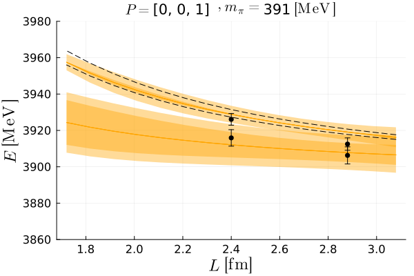
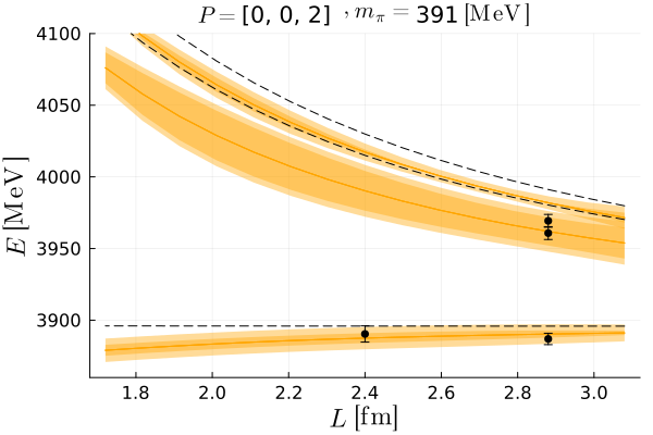
Figure 3: Results from the energy levels fit to HSC24 Whyte et al. (2024) data. Black dashed lines are the non-interacting energy levels, while orange lines are the results of our fit.

The energy levels obtained from this fit are shown in Fig. 3. We show the statistic and systematic errors in the plot. The parameters obtained are given in Table 3. One can see that the first energy level is very well described. Indeed, only with this energy level one can determine the pole position of the $T_{cc}$, since this level is the closest to the pole. Still, we include the first two energy levels in the fit. For the second one, the description is inside either the statistical or systematic error band. As can be seen, the coupling is slightly larger than the one for the analysis of Collins et al. (2024). We obtain a virtual bound state like in the previous case and also as in Whyte et al. (2024). See Table 4. In this case the state is further from the threshold, indicating that the interaction gets less attractive as the pion mass increases as noted in Padmanath and Prelovsek (2022); Collins et al. (2024). We include 12 points and obtain, $\chi^{2}/dof=1.59$.

III.1.3 Global fit

In this section, we perform a global fit, which includes the energy levels studied in the previous sections Padmanath and Prelovsek (2022); Collins et al. (2024); Whyte et al. (2024) together with the first two energy levels from CLQCD22 Chen et al. (2022), and also the scattering length data from HALQCD23 Lyu et al. (2023) and HALQCD14 Ikeda et al. (2014) , collected in Table 5.

Col.	$a$	$m_{\pi}$	$a_{0}^{-1}$	$M^{c\bar{c}}_{avg}$
HALQCD23 Lyu et al. (2023)	$0.0846$	$146$	$0.05$	$3097$
HALQCD14 Ikeda et al. (2014)	$0.0907$	$411$	$2.34$	$3070$

Table 5: Summary of the scattering length data for $DD^{*}$ for different lattice collaborations. The lattice spacing $a$ is given in fm, the inverse of the scattering length, $a_{0}^{-1}$, in fm^-1, and the masses in units of MeV.

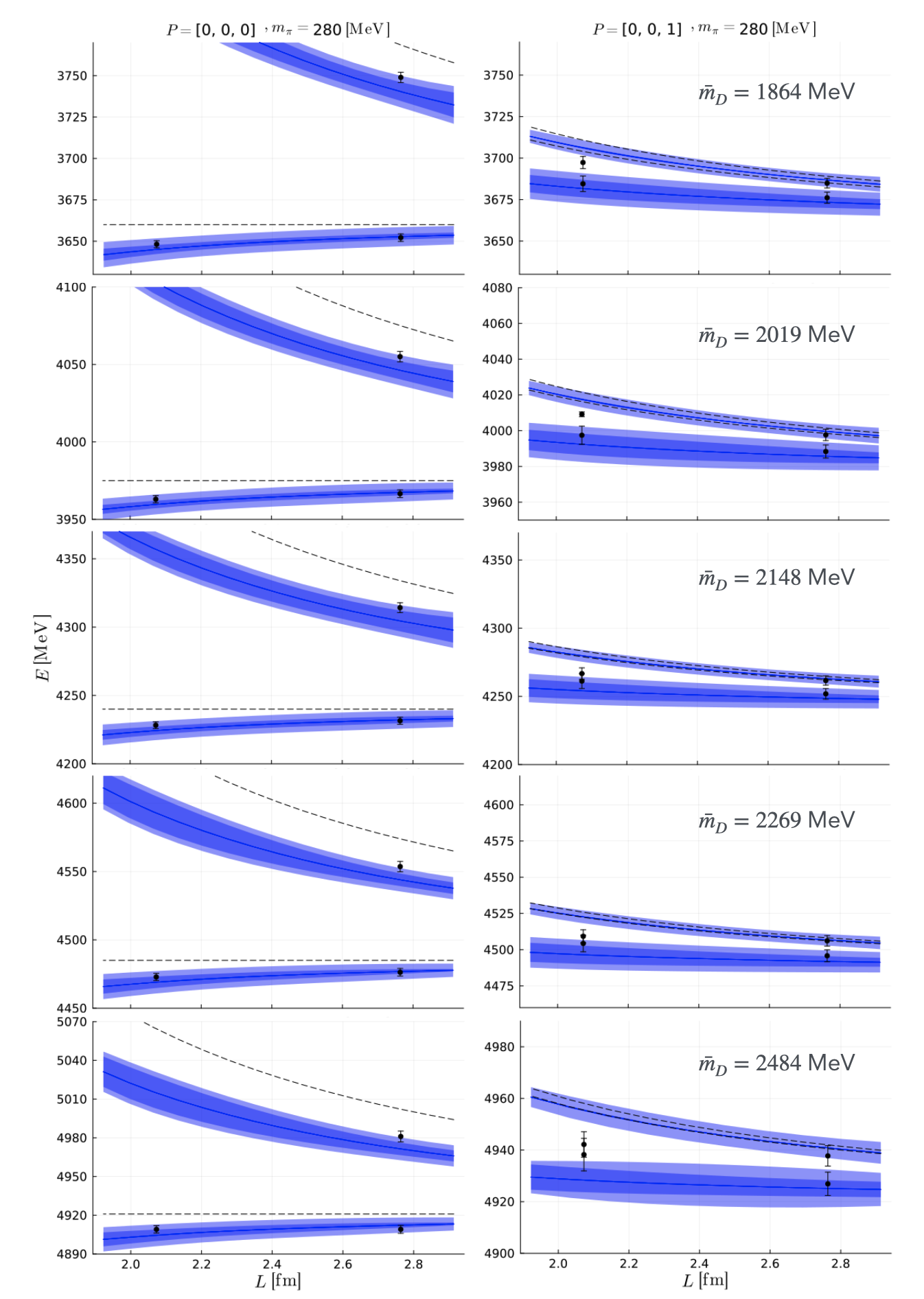
Figure 4: Results from the global fit. The five rows of plots correspond to the five sets of different charm quark mass from Collins et al. (2024). Black dashed lines are the non-interacting energy levels, while blue lines are the results of our fit.

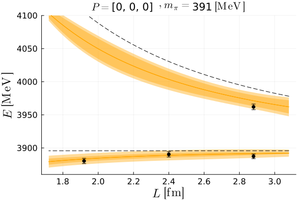
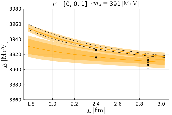
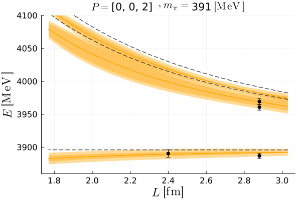
Figure 5: Results from the global fit. These plots correspond to the HSC24 Whyte et al. (2024) data. Black dashed lines are the non-interacting energy levels, while orange lines are the results of our fit.

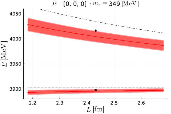
Figure 6: Results from the global fit. These plots correspond to the CLQCD22 Chen et al. (2022) data. Black dashed lines are the non-interacting energy levels, while orange lines are the results of our fit.

As we have data from several pion masses, we use the parameterization or Eq. (14) with a pion mass dependent coupling. Hence, for the global fit we have 3 parameters: the cutoff $q_{\mathrm{max}}$, $g_{1}$ and $g_{2}$ from the coupling. The values of the parameters are given in Table 3, where $g_{2}$ is given as $g_{2}m^{2}_{phys}$, to get an adimensional parameter. We obtain $q_{\mathrm{max}}=612\pm 29$ MeV, $g_{1}=3.13\pm 0.10$ and $g_{2}m^{2}_{phys}=(-0.057\pm 0.058)$. The value of $g_{1}$ obtained is close to the value of $g$ obtained in individual fits, being the pion mass dependence of the coupling mild. The results for the energy levels are depicted in Figs. 4, 5 and 6. These are very similar to the ones obtained in the individual fits. In Fig. 7 we show the phase shifts for the collaborations with energy levels. Overall, we observe a very good agreement for the first two energy levels analyzed between data and our results for energy levels and phase shifts. We determine the pole positions also in this fit at the different pion masses. These are given in Table 4. In all cases we obtain a virtual bound state. The central value of the binding energy is smaller than in the individual analysis of the Padmanath24 data, while it is larger for the HSC24 data. In any case, the result once the statistical and systematic errors are included, are compatible with the individual fits, showing consistency between the lattice data sets considered within the current errors of LQCD simulations.

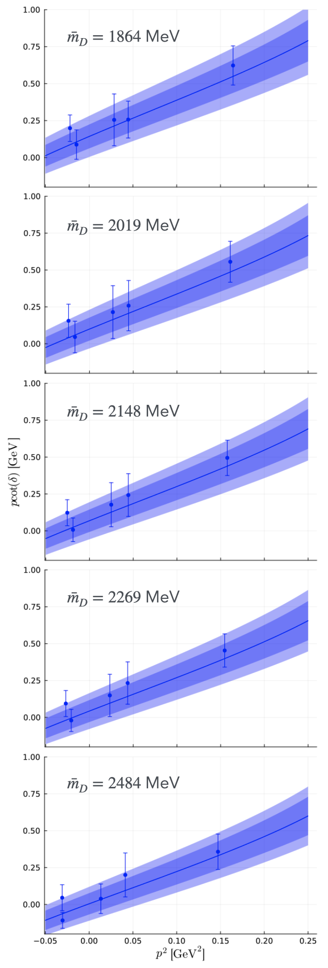
Figure 7: Phase shifts as a function of center-of-mass momentum for each collaboration. The error bands are calculated including the errors of the parameters from our fit (statistical), shown in lighter color, and the ones in in darker color (systematic), by using the errors of the meson masses of each collaboration due to the lattice spacing.

With the results of the global fit, we are ready to investigate further the quark mass dependence of the $T_{cc}(3875)^{+}$ pole position. This can be done by taking as input the study of the low-lying charmed meson masses of Gil-Domínguez and Molina (2023). In the following plots, Figs. 8 and 9, we show the result with the spin average charmonia mass at the physical point, which is $M_{avg}^{c\bar{c}}=3069$ MeV. The pion mass dependence of inverse of the scattering length is shown in Fig. 8, in comparison with the available LQCD data. We can see that this quantity increases with the pion mass and our prediction describes well the scattering LQCD data, i. e., the scattering length decreases with the pion mass. The light and heavy quark mass dependence of the pole position is given in Figs.  9 and 10. In these figures the dashed line denotes a pole in the first Riemann sheet (bound state), while the continuous line stands for the pole position in the second Riemann sheet below threshold (virtual state). In Fig. 9 (top and middle panels) we plot the binding energy of the $T_{cc}(3875)^{+}$ as a function of the pion mass. We can see that for $m_{\pi}\sim 100$ MeV, the pole changes the Riemann sheet becoming a bound state for lower pion masses. When taking into account the statistical error, the result is consistent with a bound state for the physical pion mass with a binding energy similar to the experimental one. However, note that the available LQCD data are not precise enough to determine the binding energy as precisely as the experiment does. In the middle plot, we can see that region in detail. Overall, the trend found indicates that the interaction gets less attractive as the pion mass increases. We have also shown in these two panels of Fig. 9 the result of the binding energy when rising or lowering the charm quark mass. Concretely, we plot the binding energy for $M_{\mathrm{avg}}^{c\bar{c}}=M_{\mathrm{avg}}^{c\bar{c}}|_{\mathrm{phys}}\pm 100$, the lower curve corresponding to a larger spin average charm quark mass. The result is interesting, the binding energy is affected very little by just few MeV by the change of the charm quark mass. This tells us that indeed the pole is following the threshold in such a way that the binding energy is not very sensitive to the charm quark mass. We can see that in Fig. 9 (bottom panel), where the mass of the pole is shown as a function of the pion mass for different charm quark masses, corresponding the lower curve to a smaller charm quark mass. The variation of the pole of the $T_{cc}$ mass due to a change of $50$ MeV in the spin average charm quark mass is about $52$ MeV. In the top panel of Fig. 10 we plot the binding energy as a function of the spin average charmonium mass, $M^{c\bar{c}}_{avg}$, where the gray line and error band stands for the result at the physical pion mass, while other lines denote the dependence for a fixed pion mass of the given LQCD collaboration in comparison with the LQCD data. We see a decreasing binding energy with the charm quark mass in agreement with Ref. Collins et al. (2024), meaning that the attraction gets stronger as the charm quark mass increases. In the range chosen for $M^{c\bar{c}}_{avg}$, the pole of the $T_{cc}(3875)^{+}$ becomes a bound state around the physical charm quark mass. In the bottom panel of 10 we plot the binding energy of the $T_{cc}(3875)^{+}$ as a function of the $\bar{m}_{D}=1/4(m_{D}+3m_{D^{*}})$ for all the ensembles of Collins et al. (2024), where we see a very similar behaviour with an error band consistent with the error from the data. We can also see that for $\bar{m}_{D}\gtrsim 2670$ MeV the $T_{cc}(3875)^{+}$ pole transitions to the first RS and becomes a bound state for the pion mass of Ref. Collins et al. (2024), $\sim 280$ MeV.

Figure 8: Inverse of the scattering length as a function of the pion mass. Black line is the physical trajectory extracted from our global fit.

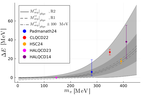
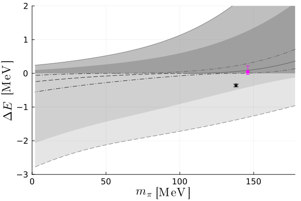
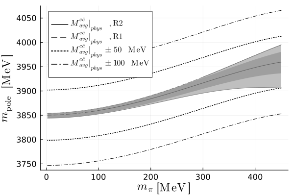
Figure 9: Binding energy of the pole associated with the $T_{cc}(3875)^{+}$ as a function of the pion mass. Black line is the physical charm quark mass trajectory extracted from the global fit. The solid line is representing a virtual bound state in the second Riemann sheet, while the dashed line denotes a bound state in the first RS. We change the sign of the binding energy when the pole is in the second RS for better clarity. The black star represents the physical binding energy from Workman et al. (2022).The CLQCD22 and HALQCD14 pole positions are calculated by us solving the equation $p\cot\delta=ip$.

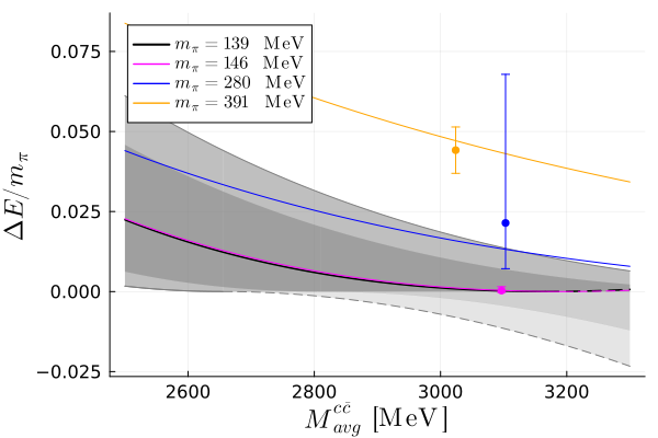
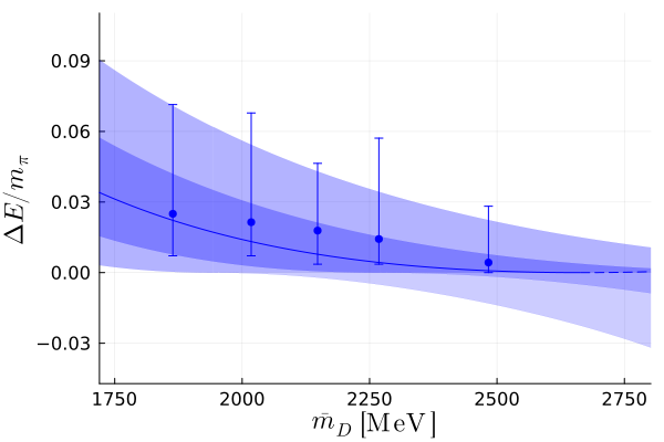
Figure 10: Top: Binding energy of the $T_{cc}(3875)^{+}$ as a function of $M^{c\bar{c}}_{avg}$ for each collaboration. Black line and error band are from the physical charm quark mass trajectory extracted from our global fit. Different lines correspond to the trajectories for different pion masses. Bottom: Binding energy of the $T_{cc}(3875)^{+}$ as a function of $\bar{m}_{D}=1/4(m_{D}+3m_{D^{*}})$ for all the ensembles of Ref. Collins et al. (2024).

III.2 Inclusion of off-shell effects and the pion exchange

In this section, we examine the effect of including an off-shell momentum dependent framework for the interaction with $\rho$-meson exchange and the pion exchange interaction on the pole position and the phase shifts in the infinite volume case.

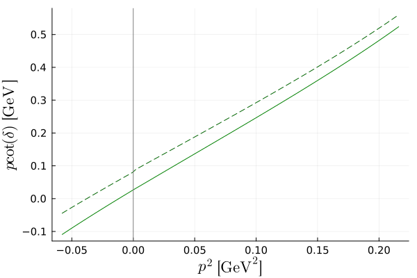
Figure 11: Comparison of the phase shifts in the physical case between the on-shell factorization (solid line) and the momentum dependent framework (dashed line).

First, we discuss the effect from considering an off-shell interaction for the vector-meson exchange potential. If one considers the momentum dependent framework, Eq. (10), with the same parameters obtained in the fit of the energy levels done in the previous subsection, one can see that the results for the scattering amplitude and phase shift changes with respect to the on-shell factorization. This effect is displayed in Fig. 11, where we observe that $p\cot{\delta}$ is lifted up in the momentum dependent framework. This variation can be absorbed in the coupling $g$. In order to get the best results that matches the LQCD data, we accommodate this variation in the coupling constant, replacing, $g_{1}\to g_{1}+0.227$ and $g_{2}m^{2}_{phys}\to g_{2}m^{2}_{phys}-0.0194$, where $g_{1}=3.13\pm 0.10$ and $g_{2}m^{2}_{phys}=-0.057\pm 0.058$, are the best parameters obtained from the global fit in Sec. III.1.3.

Now, we turn to the inclusion of the pion exchange. With this new value for the coupling $g$ in the vector meson exchange, we include the pion exchange and solve the momentum-dependent Bethe-Salpether equation, Eq. 10. In Fig. 12 (left) we compare our results with the lattice data Padmanath and Prelovsek (2022); Whyte et al. (2024); Chen et al. (2022) and we also show the physical limit extrapolation in the right panel. In this figure, the real and imaginary parts of $p\cot{\delta}$ after including the pion are depicted in red and blue colors respectively, while the result in dashed green is for only vector-meson exchange. As one can see from Fig. 12, the inclusion of the pion produces an overall decrease of $p\cot{\delta}$ while the general trend is preserved with the exception of the region close to the left-hand cut. In particular, below the left-hand cut $p\cot{\delta}$ acquires an imaginary part produced by the pion exchange while the real part diverges in agreement with what is found in Ref. Collins et al. (2024).

We can see that while the effect of the pion exchange is large around the lhc, in the rest of the energy range this effect is smaller than the phase shift error bars from the LQCD data. Still, we can have a better agreement of our momentum dependent framework including $\rho+\pi$ exchange with the LQCD data by absorbing this effect, once again, in the $g$ coupling constant. Thus, we tune the $g$ coupling to get the best possible agreement with the LQCD phase shift data outside the lhc energy region. This requires, changing $g_{1}\to g_{1}-0.351,g_{2}m^{2}_{phys}\to g_{2}m^{2}_{phys}+0.005$, where $g_{1}$ and $g_{2}$ are given by the previously calculated parameters, which are $g_{1}=3.36$ and $g_{2}m^{2}_{phys}=-0.076$. The new result is shown in Fig. 13. A similar effect of the lhc is observed. In Tab. 6 we present the new pole positions obtained including only $\rho$-meson exchange (first column), or taking into account both, $\rho+\pi$ (second column), in the momentum dependent framework of Eq. 10. As it should be, the results including only $\rho$-exchange are compatible within errors with the ones obtained in Table 4.

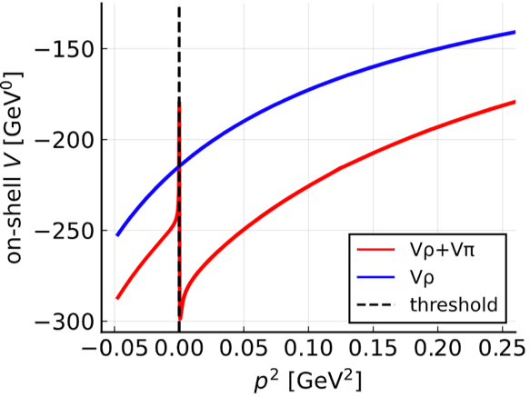
physical case CLQCD22

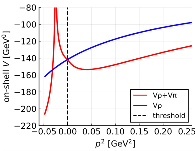
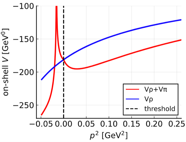
Padmanath24 HSC24

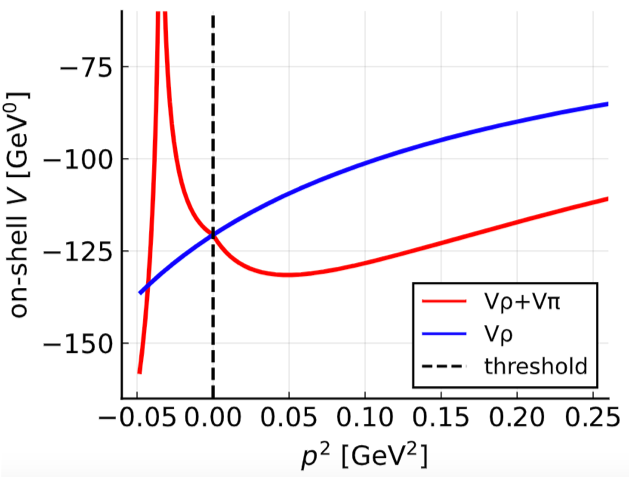
Figure 15: On-shell potential for different pion masses.

The inclusion of the pion has two visible effects. Firstly, it moves the virtual state away from the threshold if the pole is near the lhc, having a repulsive effect. This is the case of the pion mass of $280$ MeV, when this is noticeable. While if the pole is far from the lhc, the pion exchange turns out to be attractive. See Fig. 15 in the Appendix C. This occurs at the physical point. Secondly, the pion exchange causes the pole to acquire an imaginary part that increases as the pion mass becomes larger.

Finally, we depict the pion mass dependence of the pole position, real and imaginary part, including both $\rho+\pi$-meson exchanges, in Fig. 14. The dashed line of the real part of the pole denotes a bound state while the continuous line stands for a virtual state. As one can see, it becomes bound around $m_{\pi}=100$ MeV, when it turns out to be a virtual bound state transitioning into a virtual resonance state around $\sim 150$ MeV. The trend obtained here is similar to the one obtained in Ref. Abolnikov et al. (2024), implying that the effect of the one-pion exchange in the imaginary part of the pole grows with the pion mass. However, the value of the pion mass in which the state acquires imaginary part, $m_{\pi}\simeq 150$ MeV is lower in this work compared to $m_{\pi}=230$ MeV Abolnikov et al. (2024), mainly because our result is based in a chiral extrapolation of a global fit to several LQCD simulations at different pion masses ranging from $m_{\pi}=146-411$ MeV while in Abolnikov et al. (2024) the LQCD data at one pion mass, $280$ MeV, is combined with the result at the experimental point. More presice LQCD simulations are needed in the future to determine with a higher precision the quark mass dependence of doubly charm mesons.

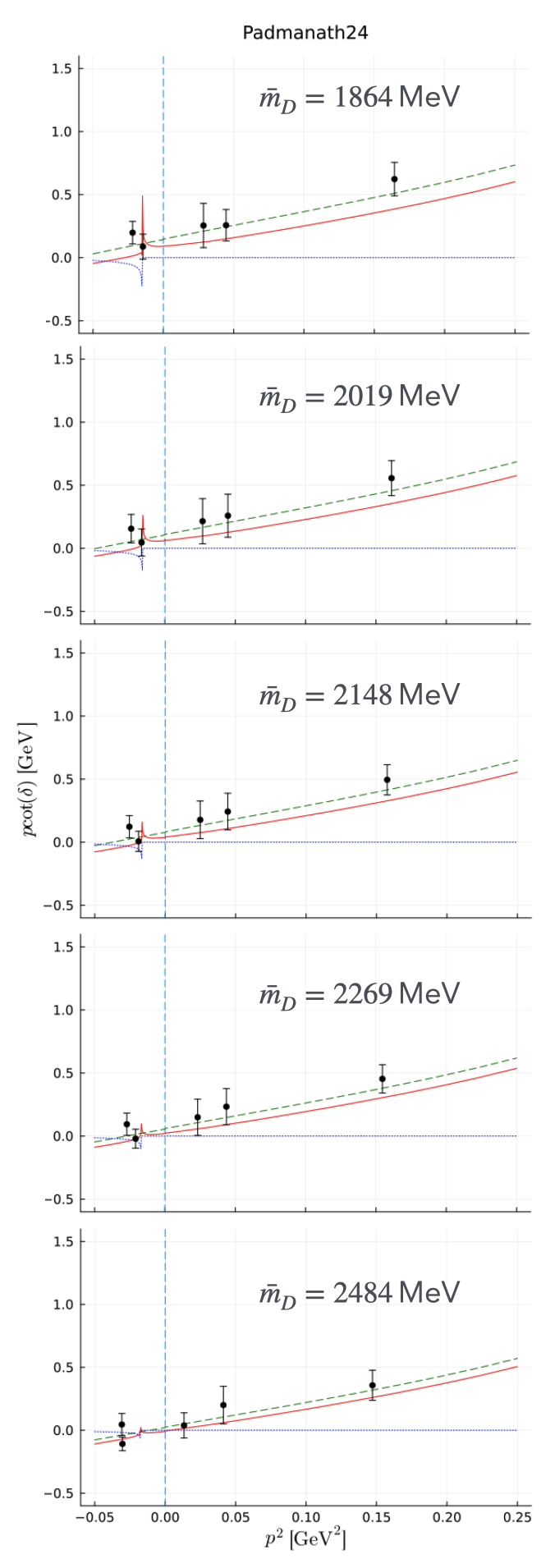
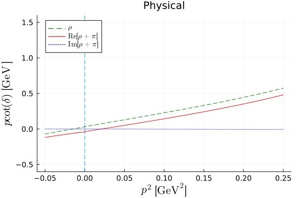
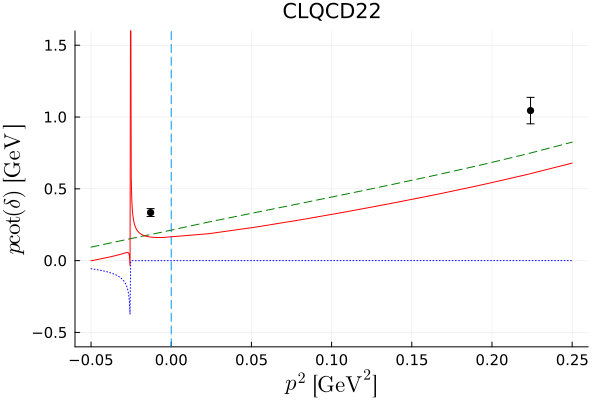
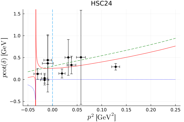
Figure 12: Comparison between the phase shifts from LQCD Padmanath and Prelovsek (2022); Whyte et al. (2024); Chen et al. (2022) and the ones obtained here by solving Eq. (10) for the $\rho$-meson exchange (green line) and the $\rho$+$\pi$ meson exchange (red and blue lines stand for real and imaginary part). The dashed vertical line denotes the $DD^{*}$ threshold. See also the explanation in the text.

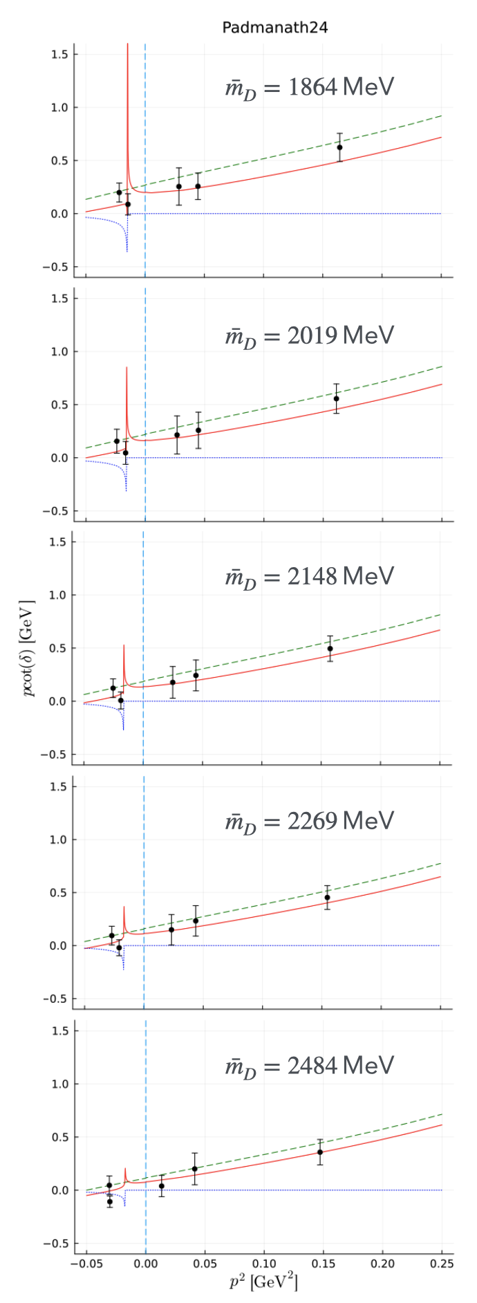
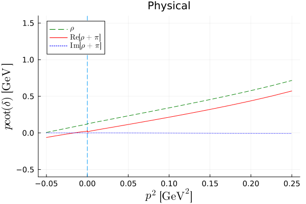
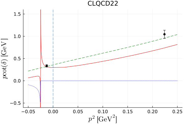
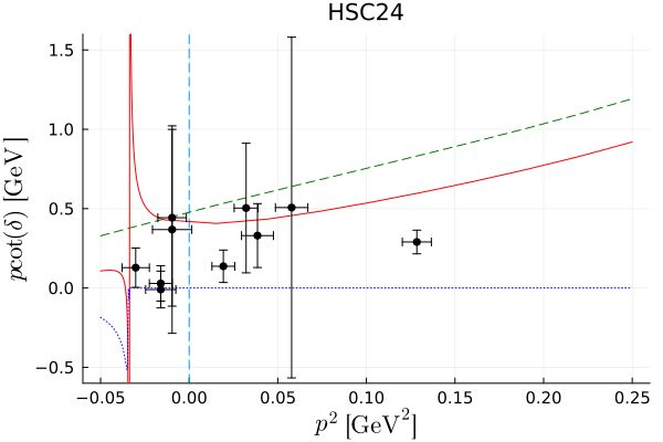
Figure 13: Similar as in Fig. 12, but readjusting the $g$ coupling to account for the pion exchange outside the lhc region as explained in the text.

Coll.		$\Delta E_{\rho}$	$\Delta E_{\rho+\pi}$
Physical		$-0.66\left({}^{+0.62}_{-0.82}\right)\left({}^{+0.20}_{-0.95}\right)$	$-0.54\left({}^{+0.52}_{-1.43}\right)\left({}^{+0.11}_{-1.08}\right)$
Padmanath24 Padmanath and Prelovsek (2022)Collins et al. (2024)	1	$-7.18\left({}^{+3.72}_{-4.81}\right)\left({}^{+2.67}_{-7.51}\right)$	$-9.37+5.85i\left({}^{+2.59-1.83i}_{-3.37+1.15i}\right)\left({}^{+3.45-3.99i}_{-5.18+0.89i}\right)$
	2	$-3.97\left({}^{+2.60}_{-3.74}\right)\left({}^{+1.31}_{-6.11}\right)$	$-7.64+4.34i\left({}^{+2.06-2.52i}_{-2.82+1.42i}\right)\left({}^{+4.49-1.80i}_{-4.50+1.12i}\right)$
	3	$-2.21\left({}^{+1.77}_{-2.95}\right)\left({}^{+0.52}_{-5.08}\right)$	$-6.4+3.04i\left({}^{+3.45-3.03i}_{-2.42+1.71i}\right)\left({}^{+2.71-0.00i}_{-3.96+1.30i}\right)$
	4	$-1.14\left({}^{+1.07}_{-2.29}\right)\left({}^{+0.53}_{-4.24}\right)$	$-5.61+1.63i\left({}^{+4.07-1.64i}_{-2.07+2.22i}\right)\left({}^{+1.51-0.01i}_{-3.51+1.47i}\right)$
	5	$-0.17\left({}^{+0.34}_{-1.26}\right)\left({}^{+0.83}_{-2.95}\right)$	$-2.37\left({}^{+2.04-0.00i}_{-3.61+2.20i}\right)\left({}^{+0.50-0.00i}_{-2.78+1.91i}\right)$
CLQCD22 Chen et al. (2022)		$-12.44\left({}^{+5.87}_{-7.35}\right)\left({}^{+5.24}_{-14.17}\right)$	$-15.87+9.20i\left({}^{+4.01-2.38i}_{-5.03+1.48i}\right)\left({}^{+6.28-6.80i}_{-9.76+1.19i}\right)$
HSC24 Whyte et al. (2024)		$-20.86\left({}^{+8.65}_{-10.36}\right)\left({}^{+9.16}_{-21.01}\right)$	$-23.37+13.19i\left({}^{+5.58-2.65i}_{-6.79+1.59i}\right)\left({}^{+6.07-9.20i}_{-14.30+1.11i}\right)$

Table 6: Comparison of the binding energy $\Delta E=E_{\text{pole}}-E_{\text{thr.}}$ in MeV calculated for different lattice collaborations and the physical point including or not the OPE. All the poles found are in the second RS.

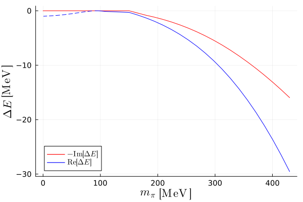
Figure 14: Dependence of the real and imaginary part of the pole with the pion mass for physical charm quark mass trajectory.

IV Conclusions

In this study, we examine data from the available LQCD simulations on $DD^{*}$ scattering, performing an extrpolation to the physical point using an EFT-based approach. For the first time, the dependence of the $T_{cc}(3875)^{+}$ pole on both light and heavy quark masses is extracted based on a global LQCD data analysis. As expected, the mass of the $T_{cc}$ increases with the charm quark mass, while the binding energy decreases, meaning that the interaction gets more attractive. Contrarily, the interaction becomes less attractive when the pion mass increases, moving the pole farther from the threshold. At the physical point, the extrapolation carried out here is compatible with the experimental $T_{cc}$ mass within statistical errors. Furthermore, we investigate the role of $\rho$ meson exchange and the potential impact of the pion. According to our analysis, the $\rho$-meson exchange is dominant but the pion contribution is non negligible. However, while the effect of the pion is clearly visible around the lhc in the scattering phase shifts, it can be reabsorbed by tunning slightly the $DD^{*}\rho$ coupling outside that region. When extracting the pole position, the imaginary part of the pole caused by the pion exchange rises with the pion mass. The real part of the pole is also affected when the pole is close to the lhc. Still, the impact of the pion exchange on the scattering phase shifts is smaller or comparable to the statistical error of the LQCD data outside the lhc. Taking into account $\rho$ and $\pi$ meson exchange, the pole evolves from a virtual bound to a virtual resonance state around $m_{\pi}=150$ MeV. The statistical and systematic uncertainties carried out in the LQCD simulations are significant in this case due to the fact that the binding energy of the $T_{cc}$ is very small. More precise LQCD data are needed in order to determine the light and heavy quark mass dependence of the pole with higher accuracy. The results obtained here strongly support that the $T_{cc}(3875)^{+}$ is dynamically generated from the $DD^{*}$ interaction.

V Acknowledgments

We acknowledge useful discussions with J. Nieves, M. Pavon-Valderrama and Pan-Pan Shi. R. Molina acknowledges support from the CIDEGENT program with Ref. CIDEGENT/2019/015 and the PROMETEU program with Ref. CIPROM/2023/59, of the Generalitat Valenciana, and also from the Spanish Ministerio de Economia y Competitividad and European Union (NextGenerationEU/PRTR) by the grant with Ref. CNS2022-13614, and from the spanish national grant PID2020-112777GB-I00. This project has received funding from the European Union’s Horizon 2020 programme No. 824093 for the STRONG-2020 project.

Appendix A The $D^{*}D\pi$ vertex

The $D^{*}D\pi$ coupling constant, $g_{D^{*}D\pi}$, can be determined by comparing the expression of the $D^{*}\to D\pi$ decay width from the Hidden Gauge Formalism (HGF) with the experimental value provided by the PDG Workman et al. (2022). The experimental decay width is given by $\Gamma\left(D^{*+}\rightarrow D\pi\right)=(82.1\pm 1.8)\,\text{keV}$ Workman et al. (2022). We take into account a form factor in the $D^{*}D\pi$ vertex for an off-shell pion with four momenta $q$ derived from QCD sum rules of exponential form, $F(q)=e^{q^{2}/\Lambda^{2}}$ Navarra et al. (2002). We set $\Lambda=1300$ MeV Molina and Oset (2020, 2023). When the pion is on-shell, $q^{2}=m_{\pi}^{2}$, we obtain $g_{D^{*}D\pi}^{\exp}=8.33\pm 0.10$, that is larger than the one predicted by the Hidden Gauge formalism, $g_{D^{*}D\pi}=\frac{m_{D^{*}}}{2f_{D}}\simeq 6.3$. In this way, the decay width obtained using the HGF, $\Gamma(D^{*+}\to D\pi)=\Gamma_{D^{*+}\to D^{0}\pi^{+}}+\Gamma_{D^{*0}\to D^{+}\pi^{0}}=\frac{1}{3}\frac{1}{8\pi}\frac{1}{m_{D^{*}}^{2}}4g_{D^{*}D\pi}^{2}F(q^{2}=m_{\pi}^{2})^{2}(q^{3}_{\pi^{+}}+\frac{q^{3}_{\pi^{0}}}{2})$, should match the experimental one at the physical point. Thus, for the $D^{*}D\pi$ vertex we take ,

$$g_{D^{*}D\pi}^{\exp}e^{q^{2}/\Lambda^{2}},\quad\Lambda=1300~{}\mathrm{MeV}\ .$$ (22)

Appendix B Polarization vectors

Explicitly, we use the following expressions for the polarization vectors:

$$\epsilon_{0}=\frac{1}{m}\begin{pmatrix}p\\ 0\\ 0\\ E_{p}\end{pmatrix}\,,\epsilon_{\pm 1}=\frac{1}{\sqrt{2}}\begin{pmatrix}0\\ \mp 1\\ -i\\ 0\end{pmatrix}\,,$$

$$\epsilon^{*}_{0}=\frac{1}{m}\begin{pmatrix}p^{\prime}\\ E_{p^{\prime}}\sin{\theta}\cos{\phi}\\ E_{p^{\prime}}\sin{\theta}\sin{\phi}\\ E_{p^{\prime}}\cos{\theta}\end{pmatrix}\,,$$

$$\epsilon^{*}_{\pm 1}=\frac{1}{\sqrt{2}}\begin{pmatrix}0\\ \mp\cos{\theta}\cos{\phi}+i\sin{\phi}\\ -i\cos{\phi}\mp\cos{\theta}\sin{\phi}\\ \pm\sin{\theta}\end{pmatrix}\,,$$ (23)

where $\vec{p}$ and $\vec{p}\,^{\prime}$ are the three-momenta of the ingoing and the outgoing vector mesons, respectively. Here the ingoing three-momenta is chosen along the z-axis, $\vec{p}=(0,0,p)$. To simplify the partial-wave projection of Eq. (6) it is convenient to exploit the azimuthal symmetry, which allows one to choose a reference frame in which the three-momentum of the outgoing vector meson lies in the $xz$-plane with $\phi=0$.

Appendix C On-shell potential plots

References

- Aaij et al. (2022a) R. Aaij et al. (LHCb), Nature Phys. 18, 751 (2022a), eprint 2109.01038.
- Aaij et al. (2022b) R. Aaij et al. (LHCb), Nature Commun. 13, 3351 (2022b), eprint 2109.01056.
- Janc and Rosina (2004) D. Janc and M. Rosina, Few Body Syst. 35, 175 (2004), eprint hep-ph/0405208.
- Yang et al. (2009) Y. Yang, C. Deng, J. Ping, and T. Goldman, Phys. Rev. D 80, 114023 (2009).
- Carames et al. (2011) T. F. Carames, A. Valcarce, and J. Vijande, Phys. Lett. B 699, 291 (2011).
- Ohkoda et al. (2012) S. Ohkoda, Y. Yamaguchi, S. Yasui, K. Sudoh, and A. Hosaka, Phys. Rev. D 86, 034019 (2012), eprint 1202.0760.
- Li et al. (2013) N. Li, Z.-F. Sun, X. Liu, and S.-L. Zhu, Phys. Rev. D 88, 114008 (2013), eprint 1211.5007.
- Liu et al. (2019) M.-Z. Liu, T.-W. Wu, M. Pavon Valderrama, J.-J. Xie, and L.-S. Geng, Phys. Rev. D 99, 094018 (2019), eprint 1902.03044.
- Liu et al. (2020) M.-Z. Liu, J.-J. Xie, and L.-S. Geng, Phys. Rev. D 102, 091502 (2020), eprint 2008.07389.
- Ader et al. (1982) J. P. Ader, J. M. Richard, and P. Taxil, Phys. Rev. D 25, 2370 (1982).
- Zouzou et al. (1986) S. Zouzou, B. Silvestre-Brac, C. Gignoux, and J. M. Richard, Z. Phys. C 30, 457 (1986).
- Heller and Tjon (1987) L. Heller and J. A. Tjon, Phys. Rev. D 35, 969 (1987).
- Silvestre-Brac and Semay (1993) B. Silvestre-Brac and C. Semay, Z. Phys. C 57, 273 (1993).
- Navarra et al. (2007) F. S. Navarra, M. Nielsen, and S. H. Lee, Phys. Lett. B 649, 166 (2007), eprint hep-ph/0703071.
- Ebert et al. (2007) D. Ebert, R. N. Faustov, V. O. Galkin, and W. Lucha, Phys. Rev. D 76, 114015 (2007), eprint 0706.3853.
- Karliner and Rosner (2017) M. Karliner and J. L. Rosner, Phys. Rev. Lett. 119, 202001 (2017), eprint 1707.07666.
- Yang et al. (2020) G. Yang, J. Ping, and J. Segovia, Phys. Rev. D 101, 014001 (2020), eprint 1911.00215.
- Tang et al. (2020) L. Tang, B.-D. Wan, K. Maltman, and C.-F. Qiao, Phys. Rev. D 101, 094032 (2020), eprint 1911.10951.
- Dong et al. (2021) X.-K. Dong, F.-K. Guo, and B.-S. Zou, Commun. Theor. Phys. 73, 125201 (2021), eprint 2108.02673.
- Chen et al. (2023) H.-X. Chen, W. Chen, X. Liu, Y.-R. Liu, and S.-L. Zhu, Rept. Prog. Phys. 86, 026201 (2023), eprint 2204.02649.
- Choi et al. (2003) S. K. Choi et al. (Belle), Phys. Rev. Lett. 91, 262001 (2003), eprint hep-ex/0309032.
- Wang et al. (2023) G.-J. Wang, Z. Yang, J.-J. Wu, M. Oka, and S.-L. Zhu (2023), eprint 2306.12406.
- Padmanath and Prelovsek (2022) M. Padmanath and S. Prelovsek, Phys. Rev. Lett. 129, 032002 (2022), eprint 2202.10110.
- Chen et al. (2022) S. Chen, C. Shi, Y. Chen, M. Gong, Z. Liu, W. Sun, and R. Zhang, Phys. Lett. B 833, 137391 (2022), eprint 2206.06185.
- Lyu et al. (2023) Y. Lyu, S. Aoki, T. Doi, T. Hatsuda, Y. Ikeda, and J. Meng, Phys. Rev. Lett. 131, 161901 (2023), eprint 2302.04505.
- Collins et al. (2024) S. Collins, A. Nefediev, M. Padmanath, and S. Prelovsek, Phys. Rev. D 109, 094509 (2024), eprint 2402.14715.
- Whyte et al. (2024) T. Whyte, D. J. Wilson, and C. E. Thomas (2024), eprint 2405.15741.
- Feijoo et al. (2021) A. Feijoo, W. H. Liang, and E. Oset, Phys. Rev. D 104, 114015 (2021), eprint 2108.02730.
- Albaladejo (2022) M. Albaladejo, Phys. Lett. B 829, 137052 (2022), eprint 2110.02944.
- Du et al. (2022) M.-L. Du, V. Baru, X.-K. Dong, A. Filin, F.-K. Guo, C. Hanhart, A. Nefediev, J. Nieves, and Q. Wang, Phys. Rev. D 105, 014024 (2022), eprint 2110.13765.
- Aaron et al. (1968) R. Aaron, R. D. Amado, and J. E. Young, Phys. Rev. 174, 2022 (1968).
- Mai et al. (2017) M. Mai, B. Hu, M. Doring, A. Pilloni, and A. Szczepaniak, Eur. Phys. J. A 53, 177 (2017), eprint 1706.06118.
- Dai et al. (2023) L. Dai, S. Fleming, R. Hodges, and T. Mehen, Phys. Rev. D 107, 076001 (2023), eprint 2301.11950.
- Fleming et al. (2007) S. Fleming, M. Kusunoki, T. Mehen, and U. van Kolck, Phys. Rev. D 76, 034006 (2007), eprint hep-ph/0703168.
- Dai et al. (2020) L. Dai, F.-K. Guo, and T. Mehen, Phys. Rev. D 101, 054024 (2020), eprint 1912.04317.
- Luscher (1986) M. Luscher, Commun. Math. Phys. 105, 153 (1986).
- Luscher (1991) M. Luscher, Nucl. Phys. B 354, 531 (1991).
- Meng et al. (2024) L. Meng, V. Baru, E. Epelbaum, A. A. Filin, and A. M. Gasparyan, Phys. Rev. D 109, L071506 (2024), eprint 2312.01930.
- Raposo and Hansen (2024) A. B. a. Raposo and M. T. Hansen, JHEP 08, 075 (2024), eprint 2311.18793.
- Bubna et al. (2024) R. Bubna, H.-W. Hammer, F. Müller, J.-Y. Pang, A. Rusetsky, and J.-J. Wu, JHEP 05, 168 (2024), eprint 2402.12985.
- Hansen et al. (2024) M. T. Hansen, F. Romero-López, and S. R. Sharpe, JHEP 06, 051 (2024), eprint 2401.06609.
- Du et al. (2024) M.-L. Du, F.-K. Guo, and B. Wu (2024), eprint 2408.09375.
- Abolnikov et al. (2024) M. Abolnikov, V. Baru, E. Epelbaum, A. A. Filin, C. Hanhart, and L. Meng (2024), eprint 2407.04649.
- Molina et al. (2010) R. Molina, T. Branz, and E. Oset, Phys. Rev. D 82, 014010 (2010), eprint 1005.0335.
- Dai et al. (2022) L. R. Dai, R. Molina, and E. Oset, Phys. Rev. D 105, 016029 (2022), [Erratum: Phys.Rev.D 106, 099902 (2022)], eprint 2110.15270.
- Bando et al. (1988) M. Bando, T. Kugo, and K. Yamawaki, Phys. Rept. 164, 217 (1988).
- Harada and Yamawaki (2003) M. Harada and K. Yamawaki, Phys. Rept. 381, 1 (2003), eprint hep-ph/0302103.
- Meissner (1988) U. G. Meissner, Phys. Rept. 161, 213 (1988).
- Nagahiro et al. (2009) H. Nagahiro, L. Roca, A. Hosaka, and E. Oset, Phys. Rev. D 79, 014015 (2009), eprint 0809.0943.
- Molina et al. (2009) R. Molina, H. Nagahiro, A. Hosaka, and E. Oset, Phys. Rev. D 80, 014025 (2009), eprint 0903.3823.
- Molina and Oset (2009) R. Molina and E. Oset, Phys. Rev. D 80, 114013 (2009), eprint 0907.3043.
- Xiao et al. (2013) C. W. Xiao, J. Nieves, and E. Oset, Phys. Rev. D 88, 056012 (2013), eprint 1304.5368.
- Molina and Oset (2020) R. Molina and E. Oset, Phys. Lett. B 811, 135870 (2020), [Erratum: Phys.Lett.B 837, 137645 (2023)], eprint 2008.11171.
- Molina and Oset (2023) R. Molina and E. Oset, Phys. Rev. D 107, 056015 (2023), eprint 2211.01302.
- Sadasivan et al. (2022) D. Sadasivan, A. Alexandru, H. Akdag, F. Amorim, R. Brett, C. Culver, M. Döring, F. X. Lee, and M. Mai, Phys. Rev. D 105, 054020 (2022), eprint 2112.03355.
- Chung (1971) S. U. Chung (1971).
- Bayar et al. (2024) M. Bayar, R. Molina, E. Oset, M.-Z. Liu, and L.-S. Geng, Phys. Rev. D 109, 076027 (2024), eprint 2312.12004.
- Workman et al. (2022) R. L. Workman et al. (Particle Data Group), PTEP 2022, 083C01 (2022).
- Doring et al. (2012a) M. Doring, U. G. Meissner, E. Oset, and A. Rusetsky, Eur. Phys. J. A 48, 114 (2012a), eprint 1205.4838.
- Gil-Domínguez and Molina (2024) F. Gil-Domínguez and R. Molina, Phys. Rev. D 109, 096002 (2024), eprint 2306.01848.
- Doring et al. (2012b) M. Doring, U. G. Meissner, E. Oset, and A. Rusetsky, Eur. Phys. J. A 48, 114 (2012b), eprint 1205.4838.
- Chen et al. (2021) R. Chen, Q. Huang, X. Liu, and S.-L. Zhu, Phys. Rev. D 104, 114042 (2021), eprint 2108.01911.
- Ikeda et al. (2014) Y. Ikeda, B. Charron, S. Aoki, T. Doi, T. Hatsuda, T. Inoue, N. Ishii, K. Murano, H. Nemura, and K. Sasaki, Phys. Lett. B 729, 85 (2014), eprint 1311.6214.
- Gil-Domínguez and Molina (2023) F. Gil-Domínguez and R. Molina, Phys. Lett. B 843, 137997 (2023), eprint 2302.12861.
- Navarra et al. (2002) F. S. Navarra, M. Nielsen, and M. E. Bracco, Phys. Rev. D 65, 037502 (2002), eprint hep-ph/0109188.