FusionRF: High-Fidelity Satellite Neural Radiance Fields from Multispectral and Panchromatic Acquisitions

Abstract

We introduce FusionRF, a novel neural rendering terrain reconstruction method from optically unprocessed satellite imagery. While previous methods depend on external pansharpening methods to fuse low resolution multispectral imagery and high resolution panchromatic imagery, FusionRF directly performs reconstruction based on optically unprocessed acquisitions with no prior knowledge. This is accomplished through the addition of a sharpening kernel which models the resolution loss in multispectral images. Additionally, novel modal embeddings allow the model to perform image fusion as a bottleneck to novel view synthesis. We evaluate our method on multispectral and panchromatic satellite images from the WorldView-3 satellite in various locations, and FusionRF outperforms previous State-of-The-Art methods in depth reconstruction on unprocessed imagery, renders sharp training and novel views, and retains multi-spectral information.

1 Introduction

Digital Surface Models allow us to visualize and understand the topology of our cities, forests, ocean floors, and plains, providing us with a digital reconstruction of the world around us. A wide array of applications, including water resource management [57], land use management [21, 38, 1], urban planning [45, 5], radio frequency planning [39], and telecommunications [19, 23] all rely on accurate reconstructions of the Earth’s surface. Historically, elevation data used to construct Digital Surface Models has been collected with complex and expensive specialized sensors and satellites, such as SAR [17, 9] and LiDAR [10]. More recently, works have begun to take advantage of the availability of optical satellite imagery data, which often spans months or years of coverage. While algorithmic methods [3, 12] depend on calibrated stereo or tri-stereo image products, neural rendering methods [16, 31, 47, 32] instead use larger datasets of commercially available satellite images to perform site reconstruction.

These neural reconstruction methods [16, 31, 32] optimize neural networks which accurately reconstruct density and radiance information from each input view, creating an implicit understanding of the scene geometry. Each method has made strides to reduce the amount of pre-processing necessary for satellite images, with the most recent method EO-NeRF [32] reducing optical pre-processing to only one step: pansharpening.

Satellite optical sensors create images by collecting light reflected from the Earth’s surface, and choose to either filter incoming light by wavelength or by spatial resolution. Multispectral images are created by a sensor with narrow sensitivity to a specific band of wavelengths, such as infrared or ultraviolet light. These images are particularly useful in disaster response [48], land development [6], water resource management [57], among many other applications. Panchromatic images are created by a sensor with broad sensitivity to the wavelengths of reflected rays which allows the sensor to resolve much finer detail on the surface of the Earth.

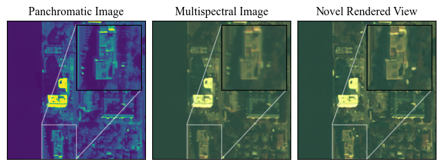
Figure 1: Result Example: Our method is able to render a novel multispectral view with additional spatial resolution by fusing the input multispectral and panchromatic image. Satellite images shown are neither color-corrected nor normalized.

The field of pansharpening attempts to fuse the spatial resolution provided by panchromatic images with the narrow wavelength bands of multispectral images to create much higher resolution multispectral images. Pansharpening approaches based on deep learning [34, 54, 13, 53] all depend on a data driven approach and collect large amounts of training data to learn from while introducing a susceptibility to poor generalization to unseen domains. As a result, pansharpening the set of multispectral and panchromatic images used for a neural reconstruction is treated as independent inference operations. This introduces the possibility of creating spectral artifacts and hallucinations [59], which are amplified if the set of scene images is out of the domain of the pansharpening algorithm. Hallucinations in input views are subsequently treated as ground truth by the downstream neural model and potentially result in inconsistent input views and disturbances in the generated surface map.

We propose FusionRF, which optimizes directly on the optically unprocessed multispectral and panchromatic imagery from the satellite source and performs image fusion as a bottleneck to producing high fidelity novel view synthesized images. Our method uses specialized modal appearance embeddings to encode the characteristics of panchromatic and multispectral views. To avoid convergence to the low resolution multispectral imagery, we incorporate a novel sparse kernel to model the spatial resolution loss in multispectral images. Jointly training the sparse kernel with the NeRF allows the model to render sharp multispectral images during inference. Image appearance embeddings are employed to resolve the radiometric differences between images, while transient embeddings in conjunction with uncertainty learning help separate transient phenomena such as cars, construction, and trees from static objects to be rendered. Together, these approaches result in more accurate 3D reconstructions of the input scene and rendered novel views which are more consistent with the input scene. This is achieved with no dependence on external pre-processing steps such as pansharpening or color correction.

Our main contributions can be summarized as follows:

• A novel satellite NeRF with an embedding strategy that enables use of full-channel multispectral and panchromatic inputs, removing the dependence on satellite image pre-processing.

• A sparse blur kernel which can resolve multispectral image resolution loss, allowing for intrinsic pansharpening within the optimization process.

• A comprehensive set of experiments to evaluate sharpness of generated views, quality of novel view synthesis, and accuracy of depth reconstruction.

2 Background

2.1 Pansharpening

To accommodate applications which require narrow specialized bandwidths of light, such as coastal, infrared, or ultraviolet imagery, satellites collect a multispectral image $I_{ms}$ which separates collected light into narrow bands, sacrificing spatial resolution. As other applications depend only on high spatial resolution, satellites employ a separate sensor that collects a broad range of wavelengths as a panchromatic image $I_{pan}$. The field of pansharpening attempts to fuse spatial and spectral resolution from both images by representing the multispectral image $I_{ms}$ as the product of a blurry convolution of the hypothetical fused image $I_{hms}$ with $h$ followed by a downsampling operation, or $I_{ms}=(I_{hms}\circledast h)\downarrow 4x$. The algorithms then attempt to reverse this process through various upsampling and fusion methods, with convolution layers taking the place of this operation in deep learning pansharpening approaches.

Pansharpened images with presumed high spectral and spatial resolution currently serve as the backbone for scene reconstruction algorithms from satellite images. The algorithms used have evolved from approximating the human optical cortex’s understanding of sharpness and color [41, 22, 40] to deep learning methods [34, 54, 13, 53]. However, these methods are dependent on large datasets, are susceptible to poor generalization, and require high training times [8], and often must be trained on downsampled data . Because no ground truth $I_{hms}$ with high spatial and spectral resolution exists, most models severely downsample $I_{ms}$ and $I_{ps}$ to create the training data and use the original $I_{ms}$ as ground truth, depending on scale-invariance to upsample $I_{ms}$ to $I_{hms}$ in inference, which is not guaranteed [14]. More recent work focuses on unsupervised learning methods [46, 26, 27, 60, 8] which operate on full resolution images. These methods are highly sensitive to the complex loss function chosen for comparing images, require a very large amount of training data, and suffer from poor generalization to unseen domains [59]. As a satellite reconstruction model uses only a few views from one small area, the perceptual errors resulting from the domain shift and any errors in the pansharpening process are amplified.

2.2 Neural Radiance Fields

Neural Radiance Field (NeRF) [36] methods attempt to encode a scene within a fully connected neural network $F_{\Theta}$:

$$F_{\Theta}(\gamma_{x}(\textbf{x}),\gamma_{d}(\textbf{d})=(\sigma,c)$$

Here, $\gamma$ represents a positional encoding which converts the camera coordinates to a higher dimensional representation. The function $F_{\Theta}$ is able to represent the scene as a combination of volume density and predicted radiance, which allows a viewer to render the scene from a novel input camera position and direction. A ray $r(t)=o+\textit{t}d$ with origin $o$ and direction $d$ is projected from each pixel in the generated image towards the scene, and classical volume rendering is used to render the predicted color by sampling $N$ locations along the ray:

$$\hat{C}(r)=\sum_{i=1}^{N}T_{i}(1-e^{-\sigma_{i}\delta{i}})\textbf{c}_{i}\;\;\text{where}\;\;T_{i}=e^{-\sum_{j=1}^{i-1}\sigma_{j}\delta_{j}}$$

Here, $T$ represents the transmittance, or the probability that the ray travels without interference, while $\delta_{i}$ represents the distance between samples. The predicted color is weighted by the transmittance and opacity of the scene. This allows the color to be controlled by the predicted scene along the entire ray, taking into account occlusions and reflections. The loss is computed as the error between the colors generated by the rendered rays and the ground truth pixel $\mathcal{L}=||\hat{C}(r)-C(r)||^{2}$.

2.3 RPC-based NeRF Models

While NeRF depends on a camera position $\textbf{x}=(x,y,z)$, images from observational satellites instead provide Rational Polynomial Coefficients (RPC). These coefficients define a geometric correction projection function for georeferencing pixels in the satellite image. While prior works such as S-NeRF [16] first estimate and replace the RPC sensor model with an approximate pinhole model, Sat-NeRF [31] samples the rays directly from the RPC sensor model. In this approach, the bounds of each ray become the maximum and minimum altitudes of the scene $h_{max}$ and $h_{min}$. Rays are then sampled by georeferencing pixel values at the minimum and maximum altitudes, sampling intermediate points during training. Both S-NeRF and Sat-NeRF rely on a shadow-aware irradiance model to render the effects of shadows, while Sat-NeRF additionally incorporates an uncertainty-learning approach similar to NeRF-W to effectively mask some of the transient objects in the scene.

EO-NeRF [47] expands upon Sat-NeRF by rendering shadows using scene geometry and sun direction instead of predicting them with a MLP head. Additionally, the model incorporates bundle adjustment within the training optimization instead of as a separate pipeline and allows the use of non color corrected satellite imagery.

2.4 NeRF Variants

Many variations on NeRF have been proposed, each of which advance the capabilities of the original method. This includes methods which incorporate bundle adjustment as part of scene optimization [25, 52, 29, 15] and utilize a multiscale representation to improve sharpness across novel views [2, 20]. NeRF-W [33] introduced a field of methods capable of recognizing and filtering out transients between views, as well as encode changes in lighting and camera properties which impact image appearance [33, 35, 49].

Some methods [28, 52, 42] address the problem of deblurring input images by modeling a blurry image as a convolution of a blur kernel with a sharp image. For a particular pixel p with color $\textbf{c}_{\textbf{p}}$, the blurry color can be calculated as $\textbf{b}_{\textbf{p}}=\textbf{c}_{\textbf{p}}\circledast h$. The blur kernel $h$ typically consists of a $K\times K$ matrix centered around $p$. However, while a typical model convolves a predicted image with $h$ to compare to the blurry ground truth, a NeRF model cannot due to the computational complexity of rendering $K^{2}\times h\times w$ rays for an image with dimensions $(h,w)$. These methods seek to resolve this issue by approximating the dense blur kernel $h$ with a small number $N$ of sparse points distributed around $p$, each with an associated weight $w$. The blurry output color can then be calculated as $\textbf{b}_{\textbf{p}}=\sum_{q\in N}\textbf{c}_{\textbf{q}}w_{\textbf{q}}$, where each ray $q$ generates a color $\textbf{c}_{\textbf{p}}$ which is then weighted by $w_{\textbf{q}}$.

DeBlur-NeRF [28] incorporates the sparse blur kernel representation within a NeRF algorithm and jointly trains a MLP to model the spatially-varying sparse kernel with the NeRF MLP. The sharp NeRF MLP $F_{\Theta}$ and blur kernel together render the blurry input images, while only using the NeRF MLP renders sharp novel images.

A recent method [44] also trains a NeRF using multispectral and panchromatic images. Additional image embeddings are included for every view that encode a function to convert predicted color $c_{RGB}$ into panchromatic color $c_{PAN}$ and computes loss against both the multispectral and panchromatic image for every ray. However, this method is spectrally inconsistent, as the panchromatic image covers a range of 450-800nm, while the R,G,and B bands together cover 450-580nm and 630-690nm [50]. As a result, the view-specific linear function is asked to reconstruct data in the missing range, which is primarily near-infrared data.

3 Method

For each input satellite view, both a multispectral image $I_{ms}$ with dimensions $(H,W)$ and panchromatic image $I_{pan}$ with dimensions $(rH,rW)$ are provided, with $r$ representing the scaling factor between the two images. Previous approaches require a pansharpening function $P$ to create an image $I_{ps}=P(I_{ms},I_{pan})$ and use this image as the input to the NeRF model, while our approach only requires a bilinear interpolation function to create $I_{lms}=\uparrow_{r}(I_{ms})$. Since both images are of the same resolution and cover the same geographic area, the pixels in each image are aligned. We model the blurring process as a convolution $I_{lms}=I_{hms}\circledast h$, where $I_{hms}$ represents a multispectral image with the same spatial resolution as $I_{pan}$. It is important to note that no image $I_{hms}$ exists, and therefore there is no ground truth high spectral and spatial resolution image to compute loss against.

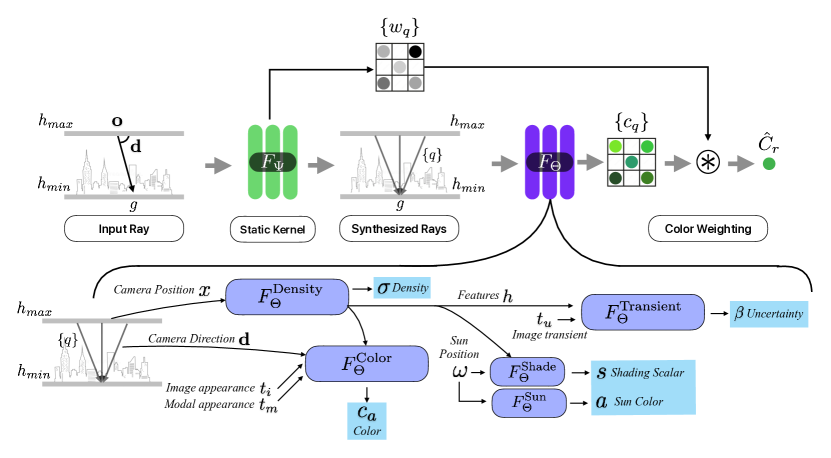
Figure 2: Our Network Architecture: Every input ray $r$ is projected from origin o in $I_{ms}$ and $I_{pan}$ to the same ground point $g$ . The sparse kernel $F_{\Phi}$ predicts weights $w_{q}$ for static locations $\{q\}$ surrounding o, which are then combined with the color predictions $\{c_{q}\}$ to produce the final output color.

3.1 RPC-based Sampling

Similarly to Sat-NeRF [31], the origin o of each ray is calculated by georeferencing the origin pixel $(r,c)$ with $h_{max}$. The destination $g$ of each ray can be calculated in kind by georeferencing $(r,c)$ with $h_{min}$. o and $g$ are converted to a geocentric coordinate system, and the direction d of each ray is calculated as:

$$\textbf{d}=\frac{g-\textbf{o}}{||g-\textbf{o}||^{2}}$$

The ray parameters o and d are then normalized to reduce the required precision for the model. Each ray can then sampled between 0 and $||g-\textbf{o}||^{2}$.

3.2 Multi Spectral NeRF

Multispectral satellite images provide wavelength information in many small ranges. In commonly available imagery from commercial satellites, this can range from 4-12 bands [56, 7, 43]. Previous approaches [16, 31, 32, 44] have required that the spectral bands be filtered to three: those that accept the primary colors red, green and blue. This means that the underlying NeRF only has access to a limited portion of the overall spectral band. In our application, since we wish to share information between the panchromatic and multispectral bands and therefore do not restrict the channel capacity of the $F_{\Theta}$ MLP [36]. For panchromatic images, we replicate the information in the panchromatic image across all channels. Our model’s MLP consists of two stages:

$$F_{\Theta}^{\text{Density}}(\gamma_{x}(\textbf{x}))=(\sigma,h)$$

where the volume density $\sigma$ is predicted as a function of the camera position x. Here, $\gamma$ represents a positional encoding which converts the camera coordinates to a higher dimensional representation. The MLP $F_{\Theta}^{\text{Color}}$ accepts features from the first stage as well as self-optimized image embeddings $t_{i}$ and $t_{m}$ and view direction d to estimate the initial color $c_{a}$:

$$F_{\Theta}^{\text{Color}}(h,\gamma_{d}(\textbf{d}),t_{m},t_{i})=(c_{a})$$

To encourage $F_{\Theta}$ to disambiguate between panchromatic and multispectral images in our dataset, we incorporate a modal embedding $t_{m}$ of size $(2,n)$, with one row dedicated to each type of imagery: multispectral or panchromatic.

We also incorporate an image-specific appearance embedding $t_{i}$ as an input to the color-producing section of the network $F_{\Theta}^{\text{Color}}$, similarly to NeRF-W [33]. This prevents appearance embedding from affecting the volume density prediction of the network, while allowing the model to remember variations in color between images.

Following S-NeRF [16], we adopt layers $F_{\Theta}^{\text{Sun}}(\omega)=a$ to predict the ambient color of shaded areas based solely on the sky position and $F_{\Theta}^{\text{Shade}}(\omega,h)=s$ to predict the impact of shadow on the rendered ray. These outputs are then combined to create a final output color:

$$c(r,\omega)=c_{a}(s+a(1-s))$$

3.3 Transient Embedding

Due to the nature of satellite orbits around the Earth, the collection times for a particular scene can span a long period. While appearance embedding attempts to capture the variations in overall lighting and photometry, a transient embedding is also employed to capture the uncertainty of each pixel in the scene [33, 31]. This is particularly useful in our case, as adapting the reconstruction loss to ignore areas of constant change such as parking lots, construction zones, and treetops allows the model to better refine static areas such as buildings. In our model the uncertainty $\beta$ is predicted through layer $F_{\Theta}^{\text{Transient}}(h,t_{u})=\beta$, similarly to NeRF-W [33] and SatNeRF [31]. The uncertainty $\beta$ attenuates the importance of a pixel in the network’s loss function:

$$\mathcal{L}=\frac{||\hat{C}({\textbf{r}})-C({\textbf{r}})_{lms}||^{2}}{2\beta_{r}^{2}}+\frac{\log(\beta_{r}+\beta_{min})+\beta_{offset}}{2}$$

This allows the model to selectively ignore pixels that it believes belong to transient objects. However, we must also check the model’s power to remove areas it does not believe it can successfully reconstruct. To do this, we add a balancing term $\log(\beta+\beta_{min})+\beta_{offset}$, with additional static parameters to prevent a negative loss.

3.4 Sparse Kernel

DeBlur-NeRF [28] introduced the idea of using multiple ray color predictions together to modeling complex motion and defocus blur. In the satellite domain, we wish to model the resolution loss caused by multispectral satellite sensors. We incorporate a sparse kernel $F_{\Psi}$ with a fixed support of 8 rays in a $2r{+}1\times 2r{+}1$ window. For a pixel $p$ with coordinates $(x,y)$, we define the fixed offsets:

$$\{q\}=\{(x+j,y+k)\mid j,k\in\{-4,0,4\}\}$$

Our $F_{\Psi}$ MLP predicts the weights:

$$(w_{\textbf{q}})=\textbf{$F_{\Psi}$}(\textbf{p},\textbf{q}^{\prime},t_{j})$$

for each $q$, which are combined in a similar way to DeBlur-NeRf:

$$\hat{C}({\textbf{r}})=\sum_{\{\textbf{r}_{\textbf{q}}\}}w_{\textbf{q}}\textbf{c}_{\textbf{q}}$$

Empirically, we find that the inclusion of $F_{\Psi}$ in this fashion allows the multispectral images rendered without a sparse kernel to be considerably sharper.

3.5 Intrinsic Pansharpening

An aligned $I_{lms}$ and $I_{pan}$ means that a ray $r$ passed through pixel $(x,y)$ will intersect the same geographic point $g$ in each image with varying resolution. Since the ray is cast through each image, loss will be computed against the same $g$ twice. For the multispectral image, the loss $\mathcal{L}_{Image}=||\hat{C}({\textbf{r}})-C({\textbf{r}})_{lms}||^{2}$ encourages the model to predict a $\hat{C}(\textbf{r})$ with a blurry color and good multispectral resolution across all 8 output channels, while the loss for the panchromatic image $\mathcal{L}_{Image}=||\hat{C}({\textbf{r}})-C({\textbf{r}})_{pan}||^{2}$ encourages the model to predict a sharp image with panchromatic color. Ideally, giving both $F_{\Psi}$ and $F_{\Theta}$ a modal embedding allows them to distinguish between the set of panchromatic $C_{pan}$ and set of multispectral $C_{ms}$ images and more effectively fuse the resolutions of both.

It is important to note that there is no requirement on the availability of panchromatic data. While a traditional pansharpening method depends on the panchromatic pair $I_{pan}$ for a multispectral image $I_{ms}$ to perform sharpening, our model is able to share information between images from the same scene through the $F_{\Theta}$ MLP. Information from the other available $I_{pan}$ images in the scene can still be applied to improve the sharpness of the rendered view of $I_{ms}$. Therefore, pansharpening within the training dataset is still possible with a limited panchromatic dataset and can even be done on novel views of the scene.

Our approach encourages the model to develop images that exactly match the original $I_{ms}$ and $I_{pan}$, removing the requirements for general metrics or downsampling. Rather than a separate operation, pansharpening becomes a bottleneck for our model to solve in the production of high quality novel views. The model’s primary task being novel view synthesis grounds the predictions to match the observed scene, reducing the likelihood of hallucinations. Since only one scene is considered in the training stage, the model cannot carry over artifacts from the domain of other scenes.

	004			068			214			260
	ERGAS $\downarrow$	PSNR $\uparrow$	SAM $\downarrow$	ERGAS $\downarrow$	PSNR $\uparrow$	SAM $\downarrow$	ERGAS $\downarrow$	PSNR $\uparrow$	SAM $\downarrow$	ERGAS $\downarrow$	PSNR $\uparrow$	SAM $\downarrow$
Ours	2.615	29.341	4.195	2.692	26.558	4.006	2.876	25.511	4.176	4.094	25.420	4.322
DPRNN	4.086	25.712	6.110	4.267	22.926	5.378	4.185	22.489	5.378	4.886	24.310	6.243
MSDCNN	4.41	24.882	7.104	4.511	22.318	5.900	4.426	21.744	5.720	5.134	23.597	7.074
PNN	6.049	22.570	9.552	5.977	20.026	8.307	5.538	20.033	8.054	6.719	21.392	9.557
DiCNN	4.453	25.215	6.743	4.786	21.988	5.627	4.738	21.507	5.862	5.815	22.913	7.039
FusionNet	3.819	26.588	5.592	4.940	21.553	5.257	4.490	21.689	4.888	4.969	24.149	5.363

Table 1: Pansharpening Results: Best result for experiment bolded. Our model is able to outperform all benchmark results while uniquely requiring no external data for training.

The model proposed by Pic et al. [44] optimizes on both multispectral and panchromatic images, relying on a linear function to convert between the R, G, and B channels and the panchromatic band. This method uses both a loss against the predicted RGB image and a loss between the converted panchromatic prediction and the original panchromatic image. In comparison, our method directly predicts the panchromatic and multispectral images, performing fusion implicitly within the NeRF. By comparing the output pixels directly against the high spatial resolution panchromatic image, we allow the model direct access to spatial resolution instead of through a learned linear function. Additionally, our method operates on all channels of a multispectral image rather than just the R, G, and B channels which allows for information in the remaining 5 bands to directly influence the panchromatic prediction. Finally, our model does not encode an explicit link between multispectral and panchromatic images, enabling training on datasets with unequal amounts of multispectral images and panchromatic images.

4 Experiments

Our method accepts $I_{ms}$ and $I_{pan}$ to create high spatial and spectral resolution output images $I_{hms}$ which are not available from current satellite technology. Therefore, no ground truth image exists to compare against. We evaluate our method by independently testing the ability to produce high quality Digital Surface Maps and sharp full resolution novel view images, as well as pansharpen the input images. For brevity, a subset of image results are shown. Expanded visuals of all datasets and experimental model details are included in the supplementary material.

In order to produce comparable results to prior work, we adopt the usage of the 2019 IEEE GRSS Data Fusion Contest [4, 24], which provided multispectral and panchromatic imagery from the WorldView-3 satellite collected over Jacksonville, Florida, USA. Four evaluation regions were chosen across both residential and industrial areas, each covering an area of $0.06$ km² with a resolution of 800x800 for panchromatic and 200x200 for multispectral imagery. The available imagery for each chosen region ranges from 11 to 24 views, and between 2 and 5 views were withheld for evaluation. A slight contrast boost was added to all images, but no color correction or normalization was performed. In order to compare directly to previous methods, we use the same bundle adjustment pipeline [30] to correct RPC coefficients before training. Unless otherwise stated, all images were rendered with a zero embedding for the appearance and transient embeddings, and the multispectral embedding for the modal embedding.

4.1 Pansharpening

	004			068			214			260
	ClipIQA $\uparrow$	BRISQUE $\downarrow$	FM $\uparrow$	ClipIQA $\uparrow$	BRISQUE $\downarrow$	FM $\uparrow$	ClipIQA $\uparrow$	BRISQUE $\downarrow$	FM $\uparrow$	ClipIQA $\uparrow$	BRISQUE $\downarrow$	FM $\uparrow$
$F_{\Psi}$ On	0.442	58.778	64.009	0.2465	53.400	68.091	0.311	36.098	57.331	0.256	48.932	85.448
$F_{\Psi}$ On - Unbalanced Data	0.372	60.182	47.463	0.227	54.264	57.181	0.280	39.580	50.247	0.282	52.349	70.837
$F_{\Psi}$ Off	0.352	66.082	53.340	0.156	61.011	51.149	0.148	47.869	56.172	0.262	61.284	64.650
$F_{\Psi}$ Off - Unbalanced Data	0.397	65.600	41.365	0.119	58.359	44.216	0.136	47.072	40.936	0.299	62.455	47.693

Table 2: No Reference Image Quality Assessment results. All results should be considered only as relative measures.

Because we intend to replace the pre-processing step of pansharpening, we compare our model’s ability to internally sharpen the input views to that of conventional deep learning based pansharpening approaches [34, 54, 13, 53]. As no ground truth $I_{hms}$ exists, these approaches take the low-resolution $I_{ms}$ as ground truth and use $\downarrow 4x(I_{ms})$ as the model input. We recreate a downsampled dataset and train and evaluate our model’s ability to pansharpen the input views against benchmark pansharpening algorithms.

We select benchmark models DRPNN [55], MSDCNN [58], PNN [34], DiCNN [18], and FusionNet [13] as the best performing deep learning models from benchmark suite [14]. Each model is trained on WorldView-3 data. We use metrics SAM, ERGAS, and PSNR [14] and find that our method achieves the best pansharpening performance as reported in Table 1, creating images with accurate color and detail to the ground truth. Examples are shown in Figure 3.

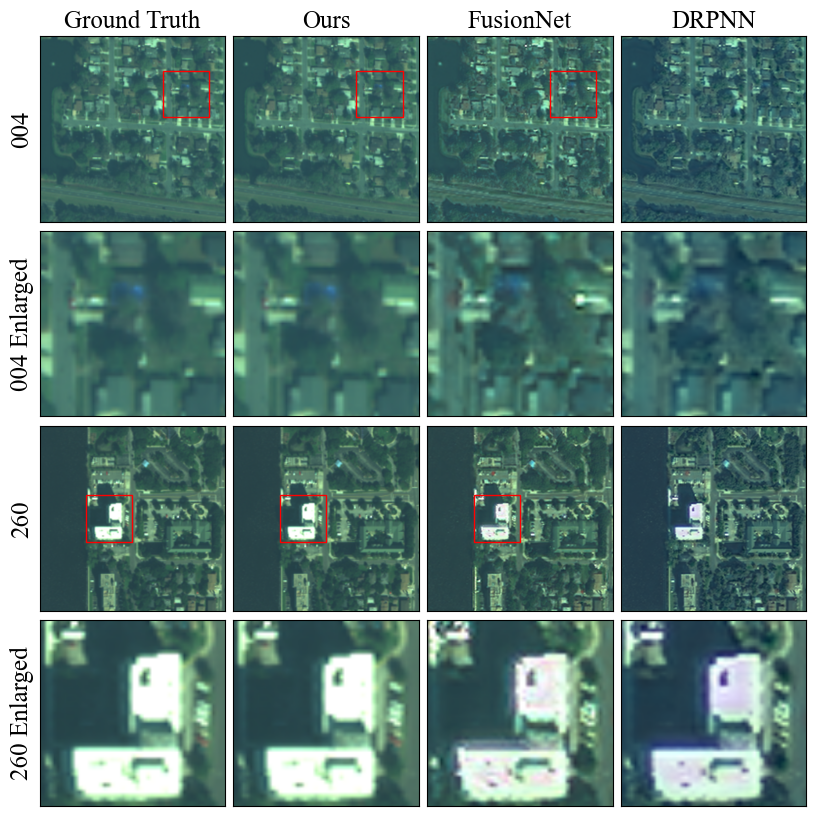
Figure 3: Pansharpening Results: DPRNN has significant color shift in rendered outputs, while FusionNet hallucinates extra details on rooftops and parking lots that were not present in the original multispectral image. Our result most closely replicates the original multispectral input.

4.2 Sharpness

To evaluate the ability of the sparse kernel to create sharper novel view images, we evaluate an ablation of our model trained without the sparse kernel. As no ground truth exists to compare rendered images against, we choose No-Reference Image Quality metrics ClipIQA [51], BRISQUE [37], and Fourier-based Frequency Domain Image Blur Measure (FM) [11]. We select ClipIQA as a deep learning approach that assesses both the quality and abstract perception of images without task-specific training and select two further algorithmic image quality benchmarks. BRISQUE operates in the spatial domain and does not rely on measures of distortion, instead looking for irregularities in the distribution of luminance across the scene. Finally, FM operates in the frequency domain to identify the proportion of high frequency areas in the scene. We use all of these metrics as relative measures of image quality between our model and an ablation that does not utilize a sparse kernel. Each model is then trained on a dataset with half of all available panchromatic images withheld. Table 2 demonstrates that the inclusion of sparse kernel $F_{\Psi}$ enables FusionRF to create sharper images on average, even when the panchromatic dataset is partially withheld. This experiment also demonstrates that because our model does not explicitly encode a pairing of panchromatic and multispectral images, our model uniquely is able to perform pansharpening on an unbalanced dataset. Enlarged examples of novel rendered views can be found in Figure 4.

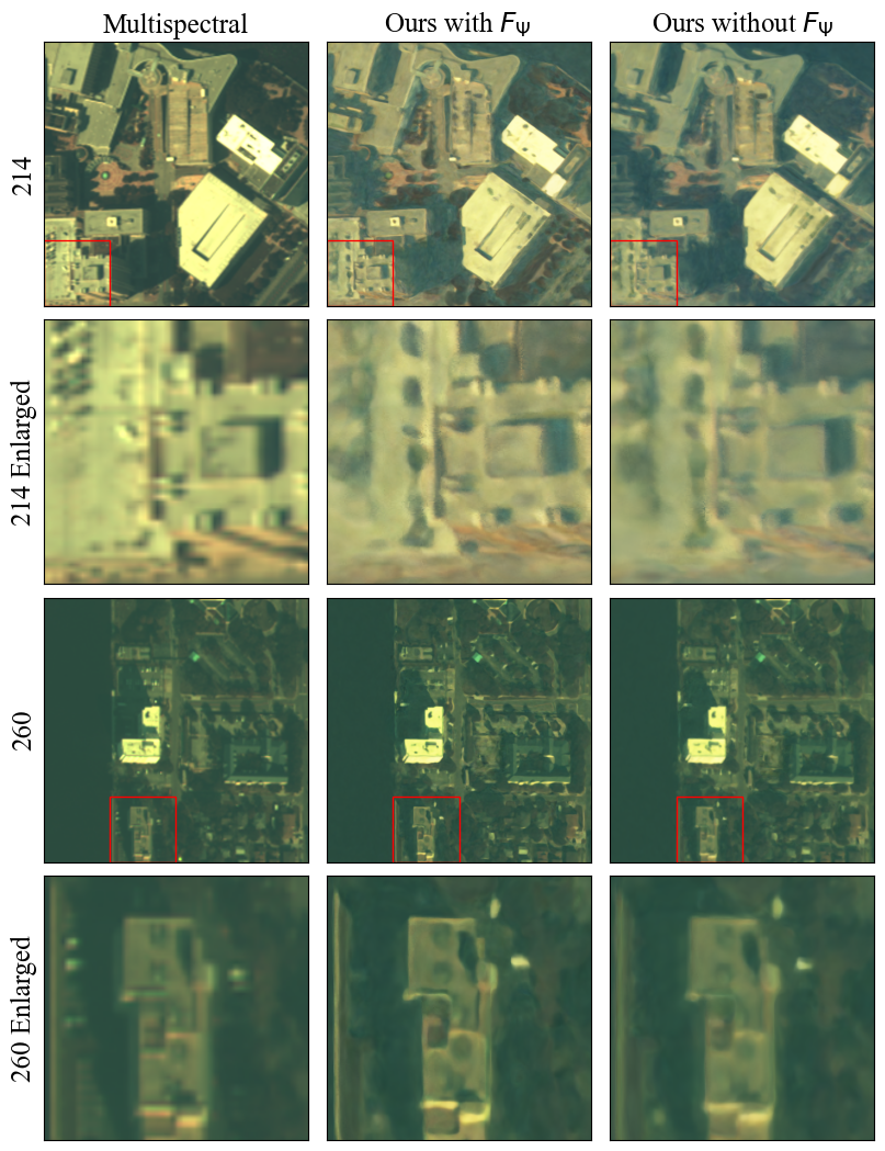
Figure 4: Sharpness Comparison Results: The results from the inclusion of the static blur kernel shows a clear enhancement in perceptual quality and sharpness compared to both the original multispectral image and an ablation of the model with no static blur kernel. Test images shown. Areas highlighted in red are enlarged in the following row.

4.3 Site Reconstruction

4.3.1 Depth

To measure of the quality of constructed site representation, we generate reconstructed depth from a training image closest to nadir with a LIDAR depth map provided in the 2019 IEEE GRSS Data Fusion Contest [4, 24]. The average error is measured with a mask applied for areas of water. For comparison, we modify previous work SatNeRF [31] by increasing the number of channels in the inner layers of the SatNeRF MLP from 3 to 8, while retaining the input pansharpened imagery. This ensures that both our model and SatNeRF-8 share input data channel sizes and spectral output resolution. The inclusion of sparse kernel as well as image and modal embeddings allows for significantly better rendering of smaller surfaces, including streets and trees. Our model produces smaller average error across all datasets as shown in Table 3, while requiring no pre-processing. Smaller details such as trees and building edges appear much more clearly defined in Figure 5.

	004	068	214	260
Ours	1.595	1.523	2.36	2.009
Ours - Without $F_{\Psi}$	1.516	1.547	2.65	2.310
SatNeRF-8	1.748	1.631	3.155	2.368

Table 3: Depth Reconstruction MAE Results: Best result for experiment bolded. On average, our method is able to outperform the best publically available satellite neural rendering method.

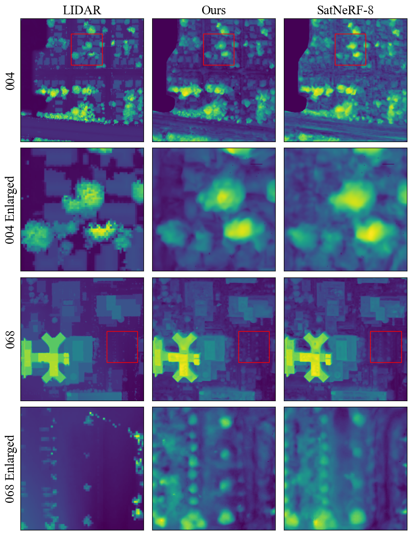
Figure 5: Depth Comparison Results: The results from our method align closer to the LIDAR ground truth, demonstrating the efficacy of our method. Areas highlighted in red are enlarged in the following row.

	004	068	214	260
Ours	30.446	25.116	22.661	24.230
Ours - Without $F_{\Psi}$	29.154	23.689	22.003	23.837
SatNeRF-8	21.695	22.551	18.802	21.714

Table 4: Novel Multispectral Synthesis PSNR Results: Best result for experiment bolded. Our method is able to outperform the modified baseline with an appropriate training image embedding.

4.3.2 Novel View Synthesis

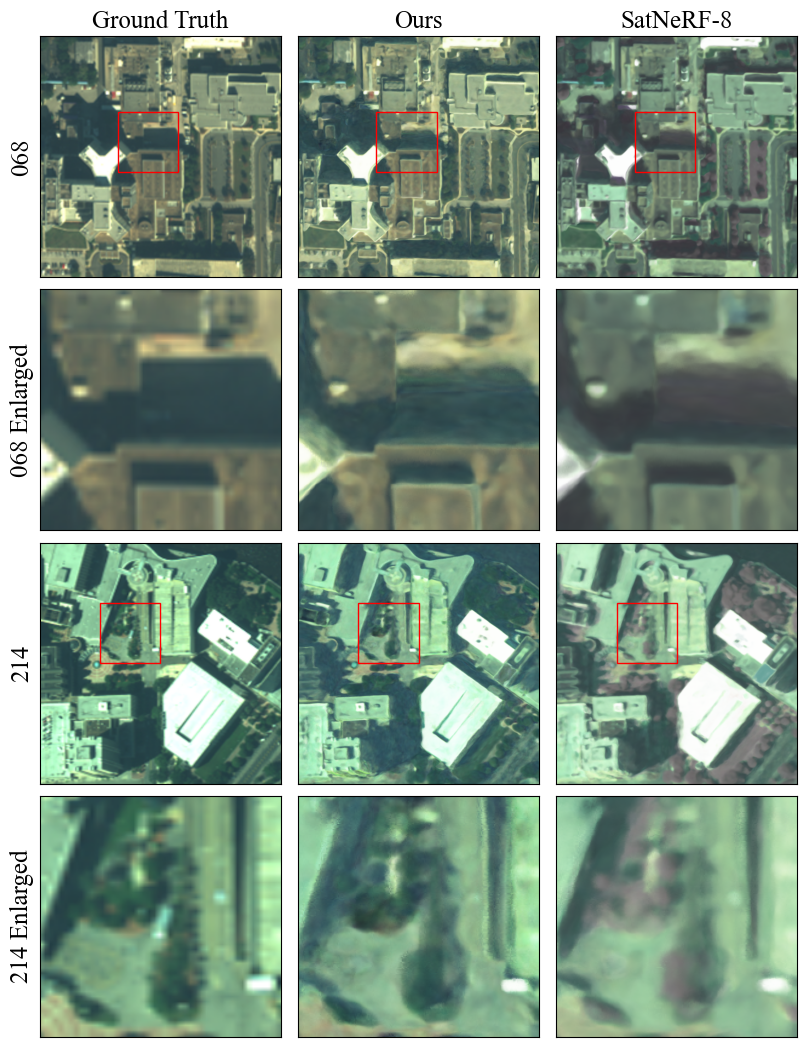
Figure 6: Novel View Rendering Results: Our method is able to more closely match the test view given an appropriate training appearance embedding.

Typical NeRF models [36, 33, 16, 31] report an perceptual image reconstruction between novel rendered views and the ground truth view. However, since no ground truth exists, we cannot report such a metric. In an effort to approximate this result, we report the PSNR between downsampled rendered novel views and the original lower resolution multispectral image, evaluating the ability of the methods to preserve the information present in the original multispectral image. For this experiment, we train the modified SatNeRF-8 on the original multispectral and panchromatic images instead of pansharpened imagery. As the input images are not radiometrically corrected, image appearance embedding greatly impacts PSNR. To compensate, we allow each image the training appearance embedding that most closely matches the luminance in the testing image.

We find that our model produces superior results to SatNeRF-8 as reported in Table 4, largely in part to the addition of appearance embeddings. As the comparison is performed on downsampled rendered images, the added sharpness from the inclusion of the blur kernel does not substantially improve the results. Figure 6 shows a comparison between novel views rendered by FusionRF and SatNeRF-8.

5 Conclusion

We present FusionRF, an advancement in satellite-based NeRF methods which removes the requirement of pansharpening in satellite image preprocessing. Our model is able to fuse low spatial resolution multispectral and low spectral resolution panchromatic imagery directly from common observation satellites and intrinsically perform pansharpening, rendering sharp novel view images with both high spectral and high spatial resolutions.

Our method outperforms previous available NeRF methods on full-channel imagery in digital surface modeling and produces novel view images closer to the original multispectral. This is achieved through novel modal embeddings which allow the model to fuse information between paired panchromatic and multispectral images while a sparse kernel resolves resolution loss in multispectral images. Our method also outperforms benchmark pansharpening algorithms on the input views. While further work can be done to increase the quality of the neural rendering, our method demonstrates that no optical preprocessing is required to generate high quality scene reconstructions from satellite images.

References

- [1] Kande RMU Bandara, Lal Samarakoon, Rajendra P Shrestha, and Yoshikazu Kamiya. Automated generation of digital terrain model using point clouds of digital surface model in forest area. Remote Sensing, 3(5):845–858, 2011.
- [2] Jonathan T Barron, Ben Mildenhall, Matthew Tancik, Peter Hedman, Ricardo Martin-Brualla, and Pratul P Srinivasan. Mip-nerf: A multiscale representation for anti-aliasing neural radiance fields. In Proceedings of the IEEE/CVF international conference on computer vision, pages 5855–5864, 2021.
- [3] Ross A Beyer, Oleg Alexandrov, and Scott McMichael. The ames stereo pipeline: Nasa’s open source software for deriving and processing terrain data. Earth and Space Science, 5(9):537–548, 2018.
- [4] Marc Bosch, Kevin Foster, Gordon Christie, Sean Wang, Gregory D Hager, and Myron Brown. Semantic stereo for incidental satellite images. In 2019 IEEE Winter Conference on Applications of Computer Vision (WACV), pages 1524–1532. IEEE, 2019.
- [5] Ansgar Brunn and Uwe Weidner. Extracting buildings from digital surface models. International Archives of Photogrammetry and Remote Sensing, 32(3 SECT 4W2):27–34, 1997.
- [6] Marshall Burke, Anne Driscoll, David B Lobell, and Stefano Ermon. Using satellite imagery to understand and promote sustainable development. Science, 371(6535):eabe8628, 2021.
- [7] Simon J. Cantrell, Jon Christopherson, Cody Anderson, Gregory L. Stensaas, Shankar N. Ramaseri Chandra, Minsu Kim, and Seonkyung Park. System characterization report on the worldview-3 imager. Report, Reston, VA, 2021.
- [8] Qi Cao, Liang-Jian Deng, Wu Wang, Junming Hou, and Gemine Vivone. Zero-shot semi-supervised learning for pansharpening. Information Fusion, 101:102001, 2024.
- [9] Yee Kit Chan and Voon Koo. An introduction to synthetic aperture radar (sar). Progress In Electromagnetics Research B, 2:27–60, 2008.
- [10] RTH Collis. Lidar. Applied optics, 9(8):1782–1788, 1970.
- [11] Kanjar De and V. Masilamani. Image sharpness measure for blurred images in frequency domain. Procedia Engineering, 64:149–158, 2013. International Conference on Design and Manufacturing (IConDM2013).
- [12] Carlo De Franchis, Enric Meinhardt-Llopis, Julien Michel, Jean-Michel Morel, and Gabriele Facciolo. An automatic and modular stereo pipeline for pushbroom images. In ISPRS Annals of the Photogrammetry, Remote Sensing and Spatial Information Sciences, 2014.
- [13] Liang-Jian Deng, Gemine Vivone, Cheng Jin, and Jocelyn Chanussot. Detail injection-based deep convolutional neural networks for pansharpening. IEEE Transactions on Geoscience and Remote Sensing, 59(8):6995–7010, 2020.
- [14] Liang-Jian Deng, Gemine Vivone, Mercedes E Paoletti, Giuseppe Scarpa, Jiang He, Yongjun Zhang, Jocelyn Chanussot, and Antonio Plaza. Machine learning in pansharpening: A benchmark, from shallow to deep networks. IEEE Geoscience and Remote Sensing Magazine, 10(3):279–315, 2022.
- [15] Tianchen Deng, Guole Shen, Tong Qin, Jianyu Wang, Wentao Zhao, Jingchuan Wang, Danwei Wang, and Weidong Chen. Plgslam: Progressive neural scene represenation with local to global bundle adjustment. In Proceedings of the IEEE/CVF Conference on Computer Vision and Pattern Recognition, pages 19657–19666, 2024.
- [16] Dawa Derksen and Dario Izzo. Shadow neural radiance fields for multi-view satellite photogrammetry. In Proceedings of the IEEE/CVF Conference on Computer Vision and Pattern Recognition, pages 1152–1161, 2021.
- [17] Rudiger Gens and John L Van Genderen. Review article sar interferometry—issues, techniques, applications. International journal of remote sensing, 17(10):1803–1835, 1996.
- [18] Lin He, Yizhou Rao, Jun Li, Jocelyn Chanussot, Antonio Plaza, Jiawei Zhu, and Bo Li. Pansharpening via detail injection based convolutional neural networks. IEEE Journal of Selected Topics in Applied Earth Observations and Remote Sensing, 12(4):1188–1204, 2019.
- [19] D.A. Holland. Os digital data for telecommunications planning. In IEE Colloquium on Terrain Modelling and Ground Cover Data for Propagation Studies, pages 2/1–2/4, 1993.
- [20] Dongting Hu, Zhenkai Zhang, Tingbo Hou, Tongliang Liu, Huan Fu, and Mingming Gong. Multiscale representation for real-time anti-aliasing neural rendering. In Proceedings of the IEEE/CVF International Conference on Computer Vision, pages 17772–17783, 2023.
- [21] Janne Järnstedt, Anssi Pekkarinen, Sakari Tuominen, Christian Ginzler, Markus Holopainen, and Risto Viitala. Forest variable estimation using a high-resolution digital surface model. ISPRS Journal of Photogrammetry and Remote Sensing, 74:78–84, 2012.
- [22] Xudong Kang, Shutao Li, and Jón Atli Benediktsson. Pansharpening with matting model. IEEE transactions on geoscience and remote sensing, 52(8):5088–5099, 2013.
- [23] Jeong Woo Kim, Dong-Cheon Lee, Jae-Hong Yom, and Jeong-Ki Pack. Telecommunication modeling by integration of geophysical and geospatial information. In IGARSS 2004. 2004 IEEE International Geoscience and Remote Sensing Symposium, volume 6, pages 4105–4108 vol.6, 2004.
- [24] Bertrand Le Saux, Naoto Yokoya, Ronny Hansch, Myron Brown, and Greg Hager. 2019 data fusion contest [technical committees]. IEEE Geoscience and Remote Sensing Magazine, 7(1):103–105, 2019.
- [25] Chen-Hsuan Lin, Wei-Chiu Ma, Antonio Torralba, and Simon Lucey. Barf: Bundle-adjusting neural radiance fields. In Proceedings of the IEEE/CVF international conference on computer vision, pages 5741–5751, 2021.
- [26] Shuyue Luo, Shangbo Zhou, Yong Feng, and Jiangan Xie. Pansharpening via unsupervised convolutional neural networks. IEEE Journal of Selected Topics in Applied Earth Observations and Remote Sensing, 13:4295–4310, 2020.
- [27] Jiayi Ma, Wei Yu, Chen Chen, Pengwei Liang, Xiaojie Guo, and Junjun Jiang. Pan-gan: An unsupervised pan-sharpening method for remote sensing image fusion. Information Fusion, 62:110–120, 2020.
- [28] Li Ma, Xiaoyu Li, Jing Liao, Qi Zhang, Xuan Wang, Jue Wang, and Pedro V Sander. Deblur-nerf: Neural radiance fields from blurry images. In Proceedings of the IEEE/CVF Conference on Computer Vision and Pattern Recognition, pages 12861–12870, 2022.
- [29] Jinjie Mai, Wenxuan Zhu, Sara Rojas, Jesus Zarzar, Abdullah Hamdi, Guocheng Qian, Bing Li, Silvio Giancola, and Bernard Ghanem. Tracknerf: Bundle adjusting nerf from sparse and noisy views via feature tracks. arXiv preprint arXiv:2408.10739, 2024.
- [30] Roger Marí, Carlo de Franchis, Enric Meinhardt-Llopis, Jérémy Anger, and Gabriele Facciolo. A generic bundle adjustment methodology for indirect rpc model refinement of satellite imagery. Image Processing On Line, 11:344–373, 2021.
- [31] Roger Marí, Gabriele Facciolo, and Thibaud Ehret. Sat-nerf: Learning multi-view satellite photogrammetry with transient objects and shadow modeling using rpc cameras. In Proceedings of the IEEE/CVF Conference on Computer Vision and Pattern Recognition, pages 1311–1321, 2022.
- [32] Roger Marí, Gabriele Facciolo, and Thibaud Ehret. Multi-date earth observation nerf: The detail is in the shadows. In Proceedings of the IEEE/CVF Conference on Computer Vision and Pattern Recognition, pages 2035–2045, 2023.
- [33] Ricardo Martin-Brualla, Noha Radwan, Mehdi SM Sajjadi, Jonathan T Barron, Alexey Dosovitskiy, and Daniel Duckworth. Nerf in the wild: Neural radiance fields for unconstrained photo collections. In Proceedings of the IEEE/CVF conference on computer vision and pattern recognition, pages 7210–7219, 2021.
- [34] Giuseppe Masi, Davide Cozzolino, Luisa Verdoliva, and Giuseppe Scarpa. Pansharpening by convolutional neural networks. Remote Sensing, 8(7):594, 2016.
- [35] Ben Mildenhall, Peter Hedman, Ricardo Martin-Brualla, Pratul P Srinivasan, and Jonathan T Barron. Nerf in the dark: High dynamic range view synthesis from noisy raw images. In Proceedings of the IEEE/CVF conference on computer vision and pattern recognition, pages 16190–16199, 2022.
- [36] Ben Mildenhall, Pratul P Srinivasan, Matthew Tancik, Jonathan T Barron, Ravi Ramamoorthi, and Ren Ng. Nerf: Representing scenes as neural radiance fields for view synthesis. Communications of the ACM, 65(1):99–106, 2021.
- [37] Anish Mittal, Anush Krishna Moorthy, and Alan Conrad Bovik. No-reference image quality assessment in the spatial domain. IEEE Transactions on Image Processing, 21(12):4695–4708, 2012.
- [38] Kimmo Nurminen, Mika Karjalainen, Xiaowei Yu, Juha Hyyppä, and Eija Honkavaara. Performance of dense digital surface models based on image matching in the estimation of plot-level forest variables. ISPRS Journal of photogrammetry and Remote Sensing, 83:104–115, 2013.
- [39] Jayesh P Pabari, Yashwant B Acharya, Uday B Desai, Shabbir N Merchant, Barla Gopala Krishna, et al. Radio frequency modelling for future wireless sensor network on surface of the moon. Int’l J. of Communications, Network and System Sciences, 3(04):395, 2010.
- [40] Chris Padwick, Michael Deskevich, Fabio Pacifici, and Scott Smallwood. Worldview-2 pan-sharpening. In Proceedings of the ASPRS 2010 Annual Conference, San Diego, CA, USA, volume 2630, pages 1–14, 2010.
- [41] Frosti Palsson, Johannes R Sveinsson, and Magnus O Ulfarsson. A new pansharpening algorithm based on total variation. IEEE Geoscience and Remote Sensing Letters, 11(1):318–322, 2013.
- [42] Cheng Peng and Rama Chellappa. Pdrf: progressively deblurring radiance field for fast scene reconstruction from blurry images. In Proceedings of the AAAI Conference on Artificial Intelligence, volume 37, pages 2029–2037, 2023.
- [43] Darius Phiri, Matamyo Simwanda, Serajis Salekin, Vincent R Nyirenda, Yuji Murayama, and Manjula Ranagalage. Sentinel-2 data for land cover/use mapping: A review. Remote Sensing, 12(14):2291, 2020.
- [44] Emilie Pic, Thibaud Ehret, Gabriele Facciolo, and Roger Marí. Pseudo pansharpening nerf for satellite image collections. In IGARSS 2024 - 2024 IEEE International Geoscience and Remote Sensing Symposium, pages 2650–2655, 2024.
- [45] Gary Priestnall, Jad Jaafar, and A Duncan. Extracting urban features from lidar digital surface models. Computers, Environment and Urban Systems, 24(2):65–78, 2000.
- [46] Ying Qu, Razieh Kaviani Baghbaderani, Hairong Qi, and Chiman Kwan. Unsupervised pansharpening based on self-attention mechanism. IEEE Transactions on Geoscience and Remote Sensing, 59(4):3192–3208, 2020.
- [47] Yingjie Qu and Fei Deng. Sat-mesh: Learning neural implicit surfaces for multi-view satellite reconstruction. Remote Sensing, 15(17):4297, 2023.
- [48] Guy JP Schumann, G Robert Brakenridge, Albert J Kettner, Rashid Kashif, and Emily Niebuhr. Assisting flood disaster response with earth observation data and products: A critical assessment. Remote Sensing, 10(8):1230, 2018.
- [49] Matthew Tancik, Vincent Casser, Xinchen Yan, Sabeek Pradhan, Ben Mildenhall, Pratul P Srinivasan, Jonathan T Barron, and Henrik Kretzschmar. Block-nerf: Scalable large scene neural view synthesis. In Proceedings of the IEEE/CVF Conference on Computer Vision and Pattern Recognition, pages 8248–8258, 2022.
- [50] Todd Updike and Chris Comp. Radiometric use of worldview-2 imagery. Technical report, DigitalGlobe, November 2010.
- [51] Jianyi Wang, Kelvin C. K. Chan, and Chen Change Loy. Exploring clip for assessing the look and feel of images, 2022.
- [52] Peng Wang, Lingzhe Zhao, Ruijie Ma, and Peidong Liu. Bad-nerf: Bundle adjusted deblur neural radiance fields. In Proceedings of the IEEE/CVF Conference on Computer Vision and Pattern Recognition, pages 4170–4179, 2023.
- [53] Shiying Wang, Xuechao Zou, Kai Li, Junliang Xing, Tengfei Cao, and Pin Tao. Towards robust pansharpening: A large-scale high-resolution multi-scene dataset and novel approach. Remote Sensing, 16(16):2899, 2024.
- [54] Yancong Wei, Qiangqiang Yuan, Xiangchao Meng, Huanfeng Shen, Liangpei Zhang, and Michael Ng. Multi-scale-and-depth convolutional neural network for remote sensed imagery pan-sharpening. In 2017 IEEE International Geoscience and Remote Sensing Symposium (IGARSS), pages 3413–3416. IEEE, 2017.
- [55] Yancong Wei, Qiangqiang Yuan, Huanfeng Shen, and Liangpei Zhang. Boosting the accuracy of multispectral image pansharpening by learning a deep residual network. IEEE Geoscience and Remote Sensing Letters, 14(10):1795–1799, 2017.
- [56] Darrel L Williams, Samuel Goward, and Terry Arvidson. Landsat. Photogrammetric Engineering & Remote Sensing, 72(10):1171–1178, 2006.
- [57] Eric F Wood, Joshua K Roundy, Tara J Troy, LPH Van Beek, Marc FP Bierkens, Eleanor Blyth, Ad de Roo, Petra Döll, Mike Ek, James Famiglietti, et al. Hyperresolution global land surface modeling: Meeting a grand challenge for monitoring earth’s terrestrial water. Water Resources Research, 47(5), 2011.
- [58] Qiangqiang Yuan, Yancong Wei, Xiangchao Meng, Huanfeng Shen, and Liangpei Zhang. A multiscale and multidepth convolutional neural network for remote sensing imagery pan-sharpening. IEEE Journal of Selected Topics in Applied Earth Observations and Remote Sensing, 11(3):978–989, 2018.
- [59] Kai Zhang, Feng Zhang, Wenbo Wan, Hui Yu, Jiande Sun, Javier Del Ser, Eyad Elyan, and Amir Hussain. Panchromatic and multispectral image fusion for remote sensing and earth observation: Concepts, taxonomy, literature review, evaluation methodologies and challenges ahead. Information Fusion, 93:227–242, 2023.
- [60] Huanyu Zhou, Qingjie Liu, and Yunhong Wang. Pgman: An unsupervised generative multiadversarial network for pansharpening. IEEE Journal of Selected Topics in Applied Earth Observations and Remote Sensing, 14:6316–6327, 2021.