Primordial neutrinos and new physics: novel approach to solving neutrino Boltzmann equation

Abstract

Understanding how hypothetical new physics influences primordial neutrinos is essential in light of interpreting past and ongoing CMB observations. To reach this goal, we present a novel approach to solving the neutrino Boltzmann equation in the Early Universe. It overcomes the limitations of existing methods by providing a model-independent, computationally efficient, and accurate framework capable of handling complex interactions and non-equilibrium neutrino distributions. We demonstrate its comprehensive applicability through several case studies. In particular, we resolve the existing discrepancy between state-of-the-art approaches regarding the dynamics of the number of ultrarelativistic degrees of freedom in the presence of injections of high-energy neutrinos.

Introduction. Primordial neutrinos play a crucial role in the evolution of the Early Universe, shaping cosmological observables. They determine the effective number of relativistic degrees of freedom, $N_{\text{eff}}$, which is a key parameter in cosmology, affecting the shape of the Cosmic Microwave Background (CMB). Their density and the energy spectrum shape define the evolution of the neutron-to-proton ratio at MeV temperatures, which sets the initial condition for Big Bang Nucleosynthesis. The same properties are important when extracting the bound on neutrino mass from cosmological observations such as baryon acoustic oscillations.

Within the standard cosmological scenario, $N_{\text{eff}}$ is predicted to be approximately $3.043$–$3.044$ [1, 2, 3, 4], and the neutrino energy spectrum follows a Fermi-Dirac distribution. Deviations from these predictions could indicate the influence of new physics on neutrino decoupling, such as the presence of Long-Lived Particles (LLPs) [5, 6, 7, 8, 9, 10, 11, 12, 13, 14, 15, 16], lepton asymmetry in the neutrino sector [10, 12], or non-standard neutrino interactions [17, 18]. Neutrinos are sensitive to these effects at temperatures up to $T\simeq 5\,\text{MeV}$, corresponding to the onset of their decoupling. Upcoming CMB experiments are expected to measure $N_{\text{eff}}$ with unprecedented precision [19, 20], offering a powerful means to either constrain or reveal new physics. Therefore, an accurate and model-independent characterization of the impact of new physics on neutrino behavior is crucial.

The central challenge is to solve the Boltzmann equation for the neutrino distribution function $f_{\nu_{\alpha}}(p,t)$ in momentum space $p$:

$$\frac{\partial f_{\nu_{\alpha}}}{\partial t}-Hp\frac{\partial f_{\nu_{\alpha}}}{\partial p}=\mathcal{I}_{\text{coll}},$$ (1)

where $H$ is the Hubble expansion rate, and $\mathcal{I}_{\text{coll}}$ represents the collision integral governing neutrino interactions. Solving this equation is highly challenging because it is a stiff integro-differential equation requiring careful tracking of spectral distortions in the neutrino distribution. The traditional approach [21, 1] involves discretizing the comoving momentum space $y=pa$ and converting the Boltzmann equation into a system of ordinary differential equations. However, this method faces two severe limitations that restrict its applicability to new physics scenarios. First, the interaction matrix elements are required to be simple analytic expressions in terms of neutrino energies. Such representations do not exist for hadronically decaying LLPs with masses above $1\,\text{GeV}$, whose decay products include quarks and gluons that undergo sequential showering and hadronization.

Second, even when analytic matrix elements are available, another significant issue arises: computational complexity. The computational time grows with the maximal neutrino energy at least as $E_{\nu}^{3}$, quickly rendering the approach impractical when high-energy neutrinos are present in the system (see, e.g., [11]). This scaling becomes even worse when more complex interactions are included, such as $2\to 3$ scatterings like $e^{+}e^{-}\to\nu\bar{\nu}\gamma$ or many-body decays of LLPs.

In this Letter, we present a novel approach to solving Eq. (1), based on the Direct Simulation Monte Carlo (DSMC) method [22, 23], which has been previously used to simulate the dynamics of rarefied gases. A detailed description of the method, along with cross-checks and case studies, can be found in the companion paper [24].

Traditional DSMC. The DSMC approach approximates the evolution of a particle system with short-range binary interactions by solving the Liouville equation for the $N$-particle distribution $F_{N}(\mathcal{R},\mathcal{V},t)$, where $\mathcal{R},\mathcal{V}$ are the phase spaces in the coordinate and velocity:

$$\frac{\partial F_{N}}{\partial t}+\sum_{i=1}^{N}\mathbf{v}_{i}\frac{\partial F_{N}}{\partial\mathbf{r}_{i}}+\sum_{1\leq i<j\leq N}\Phi_{i,j}F_{N}=0.$$ (2)

Within DSMC, the distribution function is replaced with $N$ particles. Further steps involve:

1. Reducing $F_{N}$ to a one-particle distribution by integrating over $N-1$ spatial variables.

2. Partitioning space into non-overlapping cells $\mathcal{D}^{(l)}$ containing fixed numbers of particles.

3. Implementing an iterative scheme over discrete time intervals $\Delta t$.

4. Within each time interval, splitting the evolution into particles’ free-streaming, their binary collisions within cells, and particle exchanges between cells.

Under ergodic conditions, DSMC maps onto the Bogoliubov–Born–Green–Kirkwood–Yvon hierarchy, reducing to the Boltzmann equation as $N\to\infty$ with the assumption of molecular chaos.

Let us fix the timestep $\Delta t$ to resolve characteristic interaction times:

$$\Delta t=\left(\frac{(\chi_{\text{particle}}\cdot\sigma v)_{\text{max}}\cdot N}{V_{\text{system}}}\right)^{-1},$$ (3)

where $\chi_{\text{particle}}$ is the particle weight, $V_{\text{system}}$ is the system’s volume, $\sigma$ is the cross-section, $v$ is the relative velocity, and “max” denotes the maximum over the system. Next, let us assume that the system’s volume is divided into $n_{\text{cells}}$ cells of volume $V_{\text{cell}}=V_{\text{system}}/n_{\text{cells}}$. $N_{\text{cell}}=N/n_{\text{cell}}$ is the number of particles per cell.

Simulating binary collisions within each cell may be performed within the so-called No-Time-Counter (NTC) scheme [25, 26]. We start with the following number of sampled particle pairs:

$$N_{\text{sampled}}=\frac{N_{\text{cell}}(N_{\text{cell}}-1)}{2}\frac{\omega_{\text{max}}\Delta t}{V_{\text{cell}}},$$ (4)

with $\omega_{\text{cell,max}}=(\chi_{\text{particle}}\sigma v)_{\text{cell,max}}$ being the estimate of the maximal interaction cross-section inside the cell. The interaction of each selected pair is accepted with probability

$$P_{\text{acc}}=\frac{\omega}{\omega_{\text{cell,max}}},\quad\omega=(\sigma v)_{\text{pair}}$$ (5)

Once the interaction is accepted, particles’ velocities and type change according to scattering kinematics.

Three key features make DSMC attractive. First, the computational complexity of this scheme scales linearly with $N$ [27], enabling the efficient simulation of systems with very large $N$ on modest hardware. The NTC method has been validated across various systems, including relativistic ones [28, 29, 30, 31, 32], demonstrating its robustness.

Second, DSMC may easily incorporate any interaction independently of its topology and the complexity of the matrix element. This is because of the Monte-Carlo sampling of the phase space of the reaction products, which is quite efficient and straightforward and does not require any simplifications.

Third, the scheme is conceptually very simple. It works directly with simulating particles’ interactions and does not involve complex schemes such as momentum space discretization. It automatically preserves energy in the system and is free from stability issues, which are the problems that are present in the discretization approach.

Neutrino DSMC. Let us now apply DSMC to neutrinos. Due to the homogeneity and isotropy of the Early Universe, the system is effectively zero-dimensional, with interactions occurring at a single point. Splitting it into cells is a formal step to maintain performance, and boundary interactions are neglected.

We represent neutrinos by individual particles characterized by their 4-momentum, flavor, and lepton charge. Binary interactions of neutrinos include elastic scattering with themselves and $e^{\pm}$ particles, flavor-changing annihilations like $\nu_{\alpha}\bar{\nu}_{\alpha}\to\nu_{\beta}\bar{\nu}_{\beta}$, and processes leading to neutrino creation or annihilation [33, 11].

To adapt the DSMC method for the Early Universe plasma, we incorporate key features: the Universe’s expansion, rapid equilibration of the electromagnetic (EM) sectors, quantum statistics, neutrino oscillations, and the presence of the LLPs.

The expansion is treated as an external force acting on particles and increasing the system’s volume. At each timestep $\Delta t$, we update the system volume and particle energies:

$$V_{\text{system}}\to V_{\text{system}}(1+3H\Delta t),\quad E_{i}\to\frac{E_{i}}{1+H\Delta t},$$ (6)

where $H$ is the Hubble factor and $H\Delta t\ll 1$.

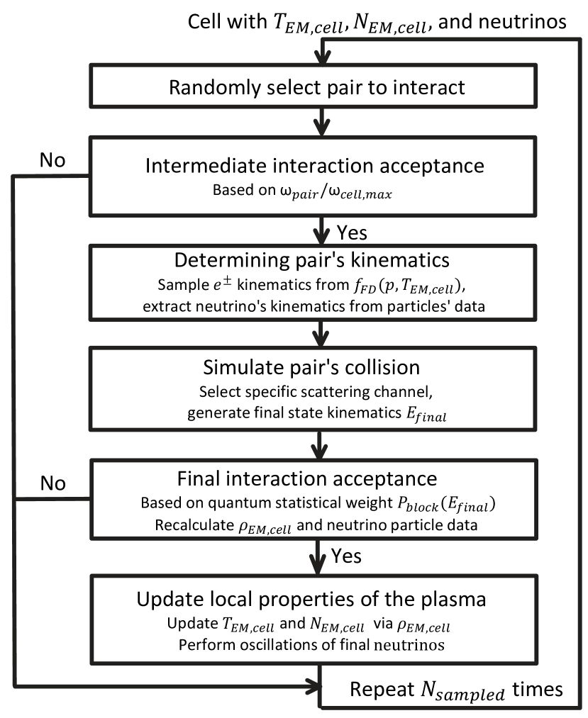
Figure 1: The Direct Simulation Monte Carlo approach we use splits the system into spatial sub-volumes called cells. To simulate the interactions of neutrinos and EM particles within the cell, we consider the so-called No-Time-Counter method from [25] and modify it by incorporating the properties of the primordial plasma. They include the instant thermalization of the electromagnetic plasma, the Pauli principle, and neutrino oscillations. All the definitions are provided in the text.

The remaining aspects modify the NTC scheme, see Fig. 1. Due to the rapid equilibration, the EM plasma may be characterized by a single quantity – temperature $T_{\text{EM}}$. To account for this, we relate the energy density of the EM plasma $\rho_{\text{EM}}$ to $T_{\text{EM}}$ both globally and locally, in each cell (where we define the local temperatures). We then sample the amounts $N_{\text{EM,cell}}$ and kinematics of interacting $e^{\pm}$ particles from the Fermi-Dirac distribution with temperature $T_{\text{EM}}$. The relation between the energy density and $T_{\text{EM}}$ is updated after any interaction with neutrinos. After simulating the interactions in all the cells, we update the global $\rho_{\text{EM}}$ and $T_{\text{EM}}$.

Neutrino oscillations are accounted for by changing the neutrino flavor $\alpha\to\beta$ at the end of each timestep with the probability given by the averaged neutrino oscillation probabilities $\langle P_{\alpha\beta}\rangle(E_{\nu},T_{\text{EM}})$ [7, 11].

Finally, the quantum statistics are included via making the final decision about interaction acceptance (on top of Eq. (5)) by computing the Pauli blocking factors for the final products. We approximate neutrino distributions entering these factors by Fermi-Dirac functions with effective temperatures $T_{\nu_{\alpha}}$ obtained from the total energy density in the cell. This is a reasonable approximation, given that the occupation number of high-energy neutrinos is $\ll 1$.

For LLPs $X$ decaying into the plasma, we introduce their number $N_{X}$, defined by the initial number density $n_{X}(t_{0})\equiv N_{X}/V_{\text{system}}$ and evolve it via

$$\Delta N_{X}(t+\Delta t)=-\frac{\Delta t}{\tau}N_{X}(t),$$ (7)

where $\tau$ is the LLP lifetime. Decay products’ phase space may be obtained via Monte Carlo simulations such as SensCalc [34] and PYTHIA8 [35], modified by incorporating the interactions of metastable decay products $\mu,\pi^{\pm},K^{\pm},K_{L}$ with the plasma, which can redistribute energy between neutrino and EM sectors [36]. Similar methods apply to non-standard scattering processes like $e^{+}e^{-}\to\nu_{\alpha}\bar{\nu}_{\alpha}\gamma$.

We have developed a proof-of-principle realization of the neutrino DSMC in Mathematica. We have tested it against existing approaches [10, 2, 14] in several well-defined scenarios, including reaching thermal equilibrium independently of the initial conditions, dynamics of neutrino temperatures under heating the neutrino or electromagnetic plasma, both including and not including the expansion of the Universe, and injections of high-energy neutrinos. The code includes a module from SensCalc allowing the simulation of the phase space of various decaying LLPs and SM particles, demonstrating its flexibility.

The performance of our neutrino DSMC already matches the traditional discretization approaches for the case of neutrino energies $E_{\nu}\sim 50-100\text{ MeV}$. Moreover, the computational time stays the same even if increasing $E_{\nu}$ up to values as large as 1 GeV and larger, where the discretization approach becomes inapplicable. The efficiency of the implementation still has the potential to be significantly improved.

Case studies. We have applied our approach in several simplified cases mimicking real physics scenarios, including the evolution of neutrinos with quasi-thermal distribution as in [10], injections of high-energy monochromatic neutrinos, and injections of neutrinos produced by secondary decays of metastable particles such as muons and mesons. Details may be found in Ref. [24]. Here, we will discuss the case of the injection of high-energy neutrinos. It corresponds to the models where we have a heavy LLP decaying into neutrinos, including Heavy Neutral Leptons (HNLs) [37, 38], neutrinophilic scalars [39], $B-L_{\alpha}$ mediators [40], and unstable relics in late reheating scenarios [5].

These scenarios are very complicated to study with state-of-the-art approaches, given the computational inefficiency outlined in the Introduction. In addition, there is an unresolved discrepancy between the existing realizations of the discretization approach in describing the dynamics of $N_{\text{eff}}$ [6, 7, 14, 15, 16]. Studying the model of HNLs with mass $m\simeq 100\text{ MeV}$, that mostly decay into (high-energy) neutrinos, some of the studies predicted an increase of $N_{\text{eff}}$, whereas the others obtained that it decreases. The difference is qualitative, and to resolve the discrepancy, an independent approach is needed. Neutrino DSMC provides such a framework, with the instant neutrino injection being the most optimal setup, combining simplicity with capturing the characteristic features of the plasma evolution.

To proceed, we introduce the quantity

$$\delta\rho_{\nu}=\left(\frac{\rho_{\nu}}{\rho_{\text{EM}}}\right)^{-1}_{\text{eq}}\frac{\rho_{\nu}}{\rho_{\text{EM}}}-1,$$ (8)

where $\rho_{\nu/\text{EM}}$ are the energy densities of neutrinos and EM plasma, and $()_{\text{eq}}$ is the standard scenario value, which is $21/22$ in the temperature limit $T\gg m_{e}$. Next, we trace its evolution under the injection of $70$ MeV neutrinos at the plasma temperature $T=3\text{ MeV}$.

The behavior of $\delta\rho_{\nu}$ is shown in Fig. 2, upper panel, where we also compare the predictions of the neutrino DSMC with the modification of [2] (see also [36]).

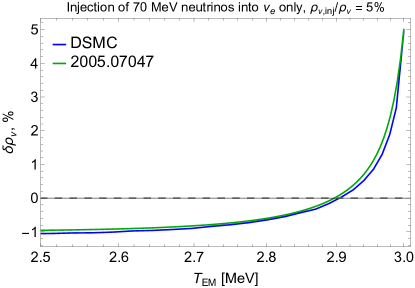
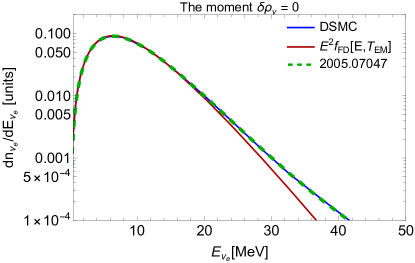
Figure 2: Evolution of the neutrino and EM plasma under the injection of 70 MeV neutrinos at the plasma temperature $T=3\text{ MeV}$, as a function of the electromagnetic temperature $T_{\text{EM}}$. We consider the injection solely into $\nu_{e}$ and fix the injected energy fraction by $\rho_{\nu,\text{inj}}/\rho_{\nu,\text{total}}=5\%$. The top panel shows the evolution of $\delta\rho_{\nu}$, given by Eq. (8). The bottom plot is the snapshot of the electron neutrino distribution spectrum at the temperature when $\delta\rho_{\nu}=0$. The blue lines are the DSMC predictions, the green lines denote the calculation by the discretization approach from [2] (see also [36]), and the red line is the shape of the would-be equilibrium spectrum. The logarithmic scale is considered to demonstrate the overabundance of the high-energy part. There are also low-energy distortions that are not visible with this scaling.

Being positive right after the injection, $\delta\rho_{\nu}$ quickly drops below. It may be understood from the properties of neutrino and EM interactions [24, 14]. First, the neutrino-EM interaction rates are orders of magnitude smaller than those within the EM sector. Therefore, the EM particles instantly thermalize, such that the spectrum of $e^{\pm}$ always has the shape of the Fermi-Dirac distribution, whereas the neutrino spectrum preserves off-equilibrium features during extended periods. Second, the neutrino-EM and neutrino-neutrino interaction rates grow with neutrino energy. Injected high-energy neutrinos either quickly pump the energy to the EM sector, or “knock out” thermal neutrinos, and these processes are much faster than those involving only thermal EM and neutrino plasma particles.

As a result of a quick transfer of the energy to the EM sector by this process, $\delta\rho_{\nu}$ instantly decreases and reaches zero value. At this moment, the neutrino spectrum still has distortions, see the lower panel of the figure. Namely, compared to the equilibrium spectrum, its high-energy part is overabundant, while the low-energy part is underabundant. This results in shifting the energy exchange balance to the EM sector, leading to the further decrease of $\delta\rho_{\nu}$ to negative values. Then, it freezes due to the expansion of the Universe.

These qualitative conclusions do not depend on the injection temperature in the range $T\gtrsim 1\text{ MeV}$, as well as on the amount of injected neutrinos and the injection pattern. They do depend on the neutrino injection energy. $\delta\rho_{\nu}$ turns negative for the injected energy as small as $E_{\nu}\simeq 35-40\text{ MeV}$. As $\delta\rho_{\nu}$ determines $N_{\text{eff}}$, our result is that is that $N_{\text{eff}}$ decreases in the presence of high-energy neutrinos. The results, both for $\delta\rho_{\nu}$ and the neutrino spectrum shape, perfectly agree with Ref. [36].

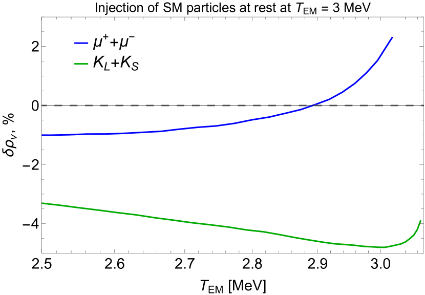
Figure 3: The impact of the injection of muons and neutral kaons at rest at $T=3\text{ MeV}$ on the quantity $\delta\rho_{\nu}$. The energy densities of $K$s and $\mu$s are fixed such that $\rho_{\text{inj}}/\rho_{\nu,\text{total}}=5\%$. It is assumed that these particles instantly decay. For the dynamics of the unstable decay products of $K$s, such as $\pi,\mu$, we assume that they lose all kinetic energy prior to decaying due to the interaction with the electromagnetic plasma [41, 42].

We have observed the same features by considering neutrinos injected by decaying muons, pions, and kaons, which may emerge as secondary particles in decays of LLPs. The behavior of $\delta\rho_{\nu}$ in the presence of some of these particles is shown in Fig. 3. Some of the existing studies utilizing such scenarios (see, e.g. [8, 9]) have to be improved to incorporate this feature.

Conclusion and outlook. We have developed a novel method to solve the neutrino Boltzmann equation in the presence of new physics. It is based on representing the neutrino distribution function with real particles and simulating their collisions using the improved Direct Simulation Monte Carlo method.

The approach provides a powerful framework for simulating neutrino decoupling in the Early Universe, overcoming the limitations of traditional approaches. Namely, it may incorporate various processes with neutrinos and Long-Lived Particles – from simple two-body decays of LLPs to neutrino non-standard interactions, $2\to n$ scatterings, and hadronic decays of LLP, for which the final phase space is computed in external tools like PYTHIA8 and SensCalc. It is also not limited by computational performance in the injection of high-energy neutrinos.

As a result, our approach can be applied to study various new physics scenarios, including those involving heavy unstable relics, dark radiation, non-standard neutrino interactions, lepton asymmetry in the neutrino spectrum, and a combination of these. Accurate modeling of these effects is essential for interpreting upcoming precision CMB measurements and exploring physics beyond the Standard Model.

Our results, in particular the impact of high-energy neutrinos on the evolution of the SM plasma, highlight the importance of accurately modeling non-equilibrium processes and high-energy interactions with neutrinos to predict cosmological observables like $N_{\text{eff}}$.

Acknowledgements. We thank Stefan Stefanov for reviewing our DSMC implementation, Fabio Peano, Luís Oliveira e Silva, and Kyrylo Bondarenko for helpful discussions, and Gideon Baur for reading the manuscript. M.O. acknowledges support from the European Union’s Horizon 2020 research and innovation program under the Marie Sklodowska-Curie grant agreement No. 860881-HIDDeN.

References

- [1] E. Grohs, G. M. Fuller, C. T. Kishimoto, M. W. Paris, and A. Vlasenko, “Neutrino energy transport in weak decoupling and big bang nucleosynthesis,” Phys. Rev. D 93 (2016) no. 8, 083522, arXiv:1512.02205 [astro-ph.CO].
- [2] K. Akita and M. Yamaguchi, “A precision calculation of relic neutrino decoupling,” JCAP 08 (2020) 012, arXiv:2005.07047 [hep-ph].
- [3] M. Cielo, M. Escudero, G. Mangano, and O. Pisanti, “Neff in the Standard Model at NLO is 3.043,” Phys. Rev. D 108 (2023) no. 12, L121301, arXiv:2306.05460 [hep-ph].
- [4] M. Drewes, Y. Georis, M. Klasen, L. P. Wiggering, and Y. Y. Y. Wong, “Towards a precision calculation of in the Standard Model III: Improved estimate of NLO corrections to the collision integral,” arXiv:2402.18481 [hep-ph].
- [5] S. Hannestad, “What is the lowest possible reheating temperature?,” Phys. Rev. D 70 (2004) 043506, arXiv:astro-ph/0403291.
- [6] A. D. Dolgov, S. H. Hansen, G. Raffelt, and D. V. Semikoz, “Heavy sterile neutrinos: Bounds from big bang nucleosynthesis and SN1987A,” Nucl. Phys. B 590 (2000) 562–574, arXiv:hep-ph/0008138.
- [7] O. Ruchayskiy and A. Ivashko, “Restrictions on the lifetime of sterile neutrinos from primordial nucleosynthesis,” JCAP 10 (2012) 014, arXiv:1202.2841 [hep-ph].
- [8] A. Fradette and M. Pospelov, “BBN for the LHC: constraints on lifetimes of the Higgs portal scalars,” Phys. Rev. D 96 (2017) no. 7, 075033, arXiv:1706.01920 [hep-ph].
- [9] A. Fradette, M. Pospelov, J. Pradler, and A. Ritz, “Cosmological beam dump: constraints on dark scalars mixed with the Higgs boson,” Phys. Rev. D 99 (2019) no. 7, 075004, arXiv:1812.07585 [hep-ph].
- [10] M. Escudero Abenza, “Precision early universe thermodynamics made simple: and neutrino decoupling in the Standard Model and beyond,” JCAP 05 (2020) 048, arXiv:2001.04466 [hep-ph].
- [11] N. Sabti, A. Magalich, and A. Filimonova, “An Extended Analysis of Heavy Neutral Leptons during Big Bang Nucleosynthesis,” JCAP 11 (2020) 056, arXiv:2006.07387 [hep-ph].
- [12] G. B. Gelmini, M. Kawasaki, A. Kusenko, K. Murai, and V. Takhistov, “Big Bang Nucleosynthesis constraints on sterile neutrino and lepton asymmetry of the Universe,” JCAP 09 (2020) 051, arXiv:2005.06721 [hep-ph].
- [13] A. Boyarsky, M. Ovchynnikov, O. Ruchayskiy, and V. Syvolap, “Improved big bang nucleosynthesis constraints on heavy neutral leptons,” Phys. Rev. D 104 (2021) no. 2, 023517, arXiv:2008.00749 [hep-ph].
- [14] A. Boyarsky, M. Ovchynnikov, N. Sabti, and V. Syvolap, “When feebly interacting massive particles decay into neutrinos: The Neff story,” Phys. Rev. D 104 (2021) no. 3, 035006, arXiv:2103.09831 [hep-ph].
- [15] L. Mastrototaro, P. D. Serpico, A. Mirizzi, and N. Saviano, “Massive sterile neutrinos in the early Universe: From thermal decoupling to cosmological constraints,” Phys. Rev. D 104 (2021) no. 1, 016026, arXiv:2104.11752 [hep-ph].
- [16] H. Rasmussen, A. McNichol, G. M. Fuller, and C. T. Kishimoto, “Effects of an intermediate mass sterile neutrino population on the early Universe,” Phys. Rev. D 105 (2022) no. 8, 083513, arXiv:2109.11176 [hep-ph].
- [17] M. Archidiacono and S. Hannestad, “Updated constraints on non-standard neutrino interactions from Planck,” JCAP 07 (2014) 046, arXiv:1311.3873 [astro-ph.CO].
- [18] F. Forastieri, M. Lattanzi, and P. Natoli, “Constraints on secret neutrino interactions after Planck,” JCAP 07 (2015) 014, arXiv:1504.04999 [astro-ph.CO].
- [19] Simons Observatory Collaboration, P. Ade et al., “The Simons Observatory: Science goals and forecasts,” JCAP 02 (2019) 056, arXiv:1808.07445 [astro-ph.CO].
- [20] CMB-S4 Collaboration, K. N. Abazajian et al., “CMB-S4 Science Book, First Edition,” arXiv:1610.02743 [astro-ph.CO].
- [21] S. Hannestad and J. Madsen, “Neutrino decoupling in the early universe,” Phys. Rev. D 52 (1995) 1764–1769, arXiv:astro-ph/9506015.
- [22] G. Bird, “Direct simulation and the boltzmann equation,” Physics of Fluids 13 (1970) no. 11, 2676–2681.
- [23] S. Stefanov, “On the basic concepts of the direct simulation monte carlo method,” Physics of Fluids 31 (2019) no. 6, .
- [24] M. Ovchynnikov and V. Syvolap, “How new physics affects primordial neutrinos decoupling: Direct Simulation Monte Carlo approach,” arXiv:2409.07378 [astro-ph.CO].
- [25] G. Bird, “Perception of numerical methods in rarefied gasdynamics,” Progress in Astronautics and Aeronautics 117 (1989) 211–226.
- [26] E. Roohi and S. Stefanov, “Collision partner selection schemes in dsmc: From micro/nano flows to hypersonic flows,” Physics Reports 656 (2016) 1–38.
- [27] M. A. Gallis, J. R. Torczynski, S. J. Plimpton, D. J. Rader, and T. Koehler, “Direct simulation monte carlo: The quest for speed.,” tech. rep., Sandia National Lab.(SNL-NM), Albuquerque, NM (United States), 2014.
- [28] D. P. Schmidt and C. J. Rutland, “A new droplet collision algorithm,” Journal of Computational Physics 164 (2000) no. 1, 62–80.
- [29] J.-S. Wu and K.-C. Tseng, “Analysis of micro-scale gas flows with pressure boundaries using direct simulation monte carlo method,” Computers & Fluids 30 (2001) no. 6, 711–735.
- [30] J.-S. Wu and Y.-Y. Lian, “Parallel three-dimensional direct simulation monte carlo method and its applications,” Computers & Fluids 32 (2003) no. 8, 1133–1160.
- [31] A. Venkattraman, A. A. Alexeenko, M. Gallis, and M. Ivanov, “A comparative study of no-time-counter and majorant collision frequency numerical schemes in dsmc,” in AIP Conference Proceedings, vol. 1501, pp. 489–495, American Institute of Physics. 2012.
- [32] F. Peano, M. Marti, L. Silva, and G. Coppa, “Statistical kinetic treatment of relativistic binary collisions,” Physical Review E—Statistical, Nonlinear, and Soft Matter Physics 79 (2009) no. 2, 025701.
- [33] A. D. Dolgov, “Neutrinos in cosmology,” Phys. Rept. 370 (2002) 333–535, arXiv:hep-ph/0202122.
- [34] M. Ovchynnikov, J.-L. Tastet, O. Mikulenko, and K. Bondarenko, “Sensitivities to feebly interacting particles: Public and unified calculations,” Phys. Rev. D 108 (2023) no. 7, 075028, arXiv:2305.13383 [hep-ph].
- [35] C. Bierlich et al., “A comprehensive guide to the physics and usage of PYTHIA 8.3,” SciPost Phys. Codeb. 2022 (2022) 8, arXiv:2203.11601 [hep-ph].
- [36] K. Akita, G. Baur, M. Ovchynnikov, and V. Syvolap, “New physics decaying into muons and mesons in MeV primordial plasma: what happens next?,” to appear (2024) , arXiv:2410.XXXXX [hep-ph].
- [37] K. Bondarenko, A. Boyarsky, D. Gorbunov, and O. Ruchayskiy, “Phenomenology of GeV-scale Heavy Neutral Leptons,” JHEP 11 (2018) 032, arXiv:1805.08567 [hep-ph].
- [38] G. Magill, R. Plestid, M. Pospelov, and Y.-D. Tsai, “Dipole Portal to Heavy Neutral Leptons,” Phys. Rev. D 98 (2018) no. 11, 115015, arXiv:1803.03262 [hep-ph].
- [39] K. J. Kelly and Y. Zhang, “Mononeutrino at DUNE: New Signals from Neutrinophilic Thermal Dark Matter,” Phys. Rev. D 99 (2019) no. 5, 055034, arXiv:1901.01259 [hep-ph].
- [40] P. Ilten, Y. Soreq, M. Williams, and W. Xue, “Serendipity in dark photon searches,” JHEP 06 (2018) 004, arXiv:1801.04847 [hep-ph].
- [41] M. Kawasaki, K. Kohri, and T. Moroi, “Big-Bang nucleosynthesis and hadronic decay of long-lived massive particles,” Phys. Rev. D 71 (2005) 083502, arXiv:astro-ph/0408426.
- [42] M. Pospelov and J. Pradler, “Metastable GeV-scale particles as a solution to the cosmological lithium problem,” Phys. Rev. D 82 (2010) 103514, arXiv:1006.4172 [hep-ph].