UTrace: Poisoning Forensics for Private Collaborative Learning

Abstract

Privacy-preserving machine learning (PPML) enables multiple data owners to contribute their data privately to a set of servers that run a secure multi-party computation (MPC) protocol to train a joint ML model. In these protocols, the input data remains private throughout the training process, and only the resulting model is made available. While this approach benefits privacy, it also exacerbates the risks of data poisoning, where compromised data owners induce undesirable model behavior by contributing malicious datasets. Existing MPC mechanisms can mitigate certain poisoning attacks, but these measures are not exhaustive. To complement existing poisoning defenses, we introduce UTrace: a framework for User-level Traceback of poisoning attacks in PPML. UTrace computes user responsibility scores using gradient similarity metrics aggregated across the most relevant samples in an owner’s dataset. UTrace is effective at low poisoning rates and is resilient to poisoning attacks distributed across multiple data owners, unlike existing unlearning-based methods. We introduce methods for checkpointing gradients with low storage overhead, enabling traceback in the absence of data owners at deployment time. We also design several optimizations that reduce traceback time and communication in MPC. We provide a comprehensive evaluation of UTrace across four datasets from three data modalities (vision, text, and malware) and show its effectiveness against 10 poisoning attacks.

1 Introduction

Privacy-preserving machine learning (PPML) [74, 73, 95, 81, 75, 4] is an emerging collaborative learning paradigm that enables multiple data owners to jointly train a machine learning (ML) model without the need to share their individual datasets directly. This approach is particularly beneficial in settings where data sharing across multiple sources is restricted due to privacy concerns and regulatory constraints, such as in the healthcare and finance sectors [30]. By enabling ML models to be trained on a diverse set of datasets, collaborative learning can help unlock the potential of ML, especially in areas where limited data availability has hindered progress.

PPML systems often rely on cryptographic techniques, such as secure multi-party computation(MPC) [74, 73, 95, 81, 75, 4], to ensure the privacy of input data during training. Some collaborative learning variants [95, 27] also utilize maliciously secure MPC to provide robustness in the presence of adversarial clients. While these techniques prevent clients from deviating from the protocol, they remain vulnerable to data poisoning attacks [18] where adversaries introduce manipulated input data to influence the outcome of the ML models. Mitigating these attacks is particularly challenging in PPML, where conventional remedies, such as data sanitization methods [19, 92, 94, 42], are not directly applicable due to privacy constraints. Although some existing approaches in PPML, such as privacy-preserving input checks [69, 9, 17] or ensemble training [18], can help mitigate certain poisoning attacks, they cannot prevent all forms of data poisoning, leaving models susceptible to manipulation.

To secure the ML lifecycle, we argue that a defense-in-depth strategy is needed. This approach involves implementing multiple layers of defense during both the training and deployment phases. During deployment, mechanisms for detecting malicious activity and enforcing accountability (e.g., forensic analysis) must be in place to ensure the reliability and trustworthiness of ML models. Poisoning traceback [88] is a post-deployment mechanism which facilitates forensic investigations by identifying and tracing the origins of a poisoning attack back to specific training samples. For instance, if a model shows unexpected behavior, these tools can pinpoint the exact malicious samples responsible. By integrating reactive tools like traceback during deployment, we can ensure accountability and attribution, consequently enhancing the trustworthiness of ML.

Existing poisoning traceback methods typically employ approximate unlearning methods [88, 70] or sample-level gradient similarity metrics [40]. However, in PPML, conducting traceback at the user level is often more relevant for forensic purposes and accountability, as it identifies which parties contributed corrupted data. User-level traceback is also more suitable in PPML settings because it avoids exposing detailed information about specific data points, preserving privacy. The only existing poisoning traceback method for PPML [70] is based on approximate unlearning, and it faces scalability issues when handling poisoning attacks spread across multiple data owners.

In this paper, we introduce UTrace, a framework for user-level traceback of poisoning attacks in secure collaborative learning. We perform an analysis of unlearning-based traceback methods such as [70] and design new poisoning attacks against them to highlight their inherent limitations. Based on these insights, we design UTrace to compute user-level responsibility scores using gradient similarity metrics. When a misclassification event is observed at deployment time, the traceback procedure computes user responsibility scores by aggregating gradient similarity scores between the misclassification event and each sample of the user’s dataset. We identify challenges of aggregating sample-level scores to create user responsibility scores, particularly at low poisoning rates, and we design methods that identify the most relevant samples in an owner’s dataset for aggregation. To enable poisoning traceback in the absence of data owners at deployment time, we introduce novel checkpointing methods that rely on storing final-layer gradients and random gradient projections to reduce the amount of storage needed for traceback. Additionally, we introduce several optimizations that enable the practical deployment of our traceback tool in MPC.

Contributions. We make the following contributions:

Novel User-Level Traceback Framework. We present UTrace, a novel framework for user-level traceback of data poisoning attacks in PPML. UTrace uses gradient similarity-based responsibility scores to rank and identify anomalously influential users given an observed misclassification event.

Analysis of Unlearning-based Methods. We conduct a careful examination of existing unlearning-based traceback methods such as [70] in PPML. We discover multiple vulnerabilities in these methods and demonstrate the existence of poisoning attacks that evade these methods. Through our analysis, we demonstrate the need for more resilient approaches to traceback in collaborative learning.

Extensive Evaluation in Multiple Modalities. We provide a rigorous empirical evaluation of UTrace across three data modalities, including vision, text, and malware, four datasets, and 10 poisoning attacks. Our results indicate that UTrace is capable of detecting poisoning attacks effectively across a diverse range of data modalities.

Optimizations for Practical MPC Deployment. UTrace introduces several key optimizations in MPC making it practical for performing efficient user-level traceback while preserving training data privacy.

2 Background and Related Work

We introduce relevant background on MPC, PPML, and data poisoning attacks, after which we discuss related work.

2.1 Secure Multi-Party Computation

Secure multi-party computation (MPC) [34, 10, 47, 28] allows a set of $n$ parties to compute a function $f$ on their inputs $(x_{i})_{i\in[n]}$ without revealing any more information than can be inferred from the output of the computation. MPC has recently received attention in the context of privacy-preserving machine learning (PPML) to achieve private and secure training and inference [74, 73, 95, 81, 75, 4]. Typically, this process follows the outsourced computation paradigm, which involves a secret-sharing phase from a set of data owners (which can be many) to a set of servers (typically small).

2.2 Data Poisoning Attacks

In a data poisoning attack, an adversary with control over a fraction of the training data injects malicious samples into the training dataset in order to induce undesirable behavior in the trained model. Poisoning attacks have been studied for a large number of ML tasks [48, 14, 68, 80], but we focus on poisoning against classification [38, 87, 5, 32].

The most commonly studied form of poisoning is a backdoor attack, in which the adversary’s objective is to make the victim misclassify samples containing a particular perturbation (the “trigger”) while preserving behavior on inputs not containing the trigger [38, 86, 84, 35, 91]. Other common attack objectives include instance-targeted attacks, in which the adversary seeks to induce specific model predictions on a small set of pre-selected victim inputs [87, 5, 32, 58, 57], and indiscriminate attacks, in which the adversary reduces the overall accuracy of the classifier [68, 67, 93].

2.3 Related Work

Poisoning Defenses. In response to poisoning attacks, an extensive body of work has emerged to harden the training process. Existing defenses can be broadly categorized into two groups: heuristic defenses and certified defenses.

Heuristic defenses typically leverage certain assumptions about the clean training data, or the nature of the poisoning attack [29, 97, 94, 64, 77, 48]. Some methods directly identify and remove malicious samples. Techniques considered by prior work include spectral analysis of sample gradients [29] or intermediate network activations [94]. Other methods mitigate the impact of poisoning as a post-training step. Example techniques include pruning uninformative neurons [64] or training on randomized labels [44] followed by clean fine-tuning.

Certified defenses provide provable guarantees on the stability of classifier predictions subject to small changes to the training set within some perturbation model. These defenses produce a certificate specifying a lower bound on the dataset perturbation required for a certain decrease in test accuracy. Currently, most certified methods work by training a large ensemble of models along with some transformation to the training data [96, 50, 20, 60, 98, 82, 101]. Other works achieve certification through a careful analysis of a particular learning algorithm [83, 36, 90]. For example, [90] maintains parameter-space bounds during training, and [83] derives a closed-form certificate for linear regression under label-flipping attacks.

Poisoning Traceback. A recent line of work on poisoning traceback complements existing defenses. Our work focuses on a recent setting [88, 40, 70] that aims to identify the source of poisoning attacks. Early works [88, 40] consider the problem of identifying training samples causing a malicious misclassification, and [70] consider traceback in MPC. We discuss these works in more detail in Section 4.1. Other works [13, 52] address poisoning traceback in federated learning. Other forensic settings for poisoning include reconstructing backdoor triggers [24] and traceback for privacy violations [63].

3 Problem Statement and Threat Model

We describe the considered PPML scenario and define the task of user-level poisoning traceback. We then introduce the threat model and outline the main goals and challenges in designing our user-level traceback method.

3.1 Problem Statement

We consider a PPML training scenario in which data owners, model owners, and traceback providers coordinate to provide a classification service to clients that offers secure model training, inference, and traceback of malicious data owners.

PPML scenario. Figure 1 illustrates the general setup for PPML we consider. A set of several model owners host an ML service within a domain. For example, model owners might host a network threat detection tool for identifying malicious network activity from traffic logs containing private user information, or a cancer detection tool whose inputs contain private patient data. Such settings are typically subject to strict regulations restricting data use and sharing [2, 3].

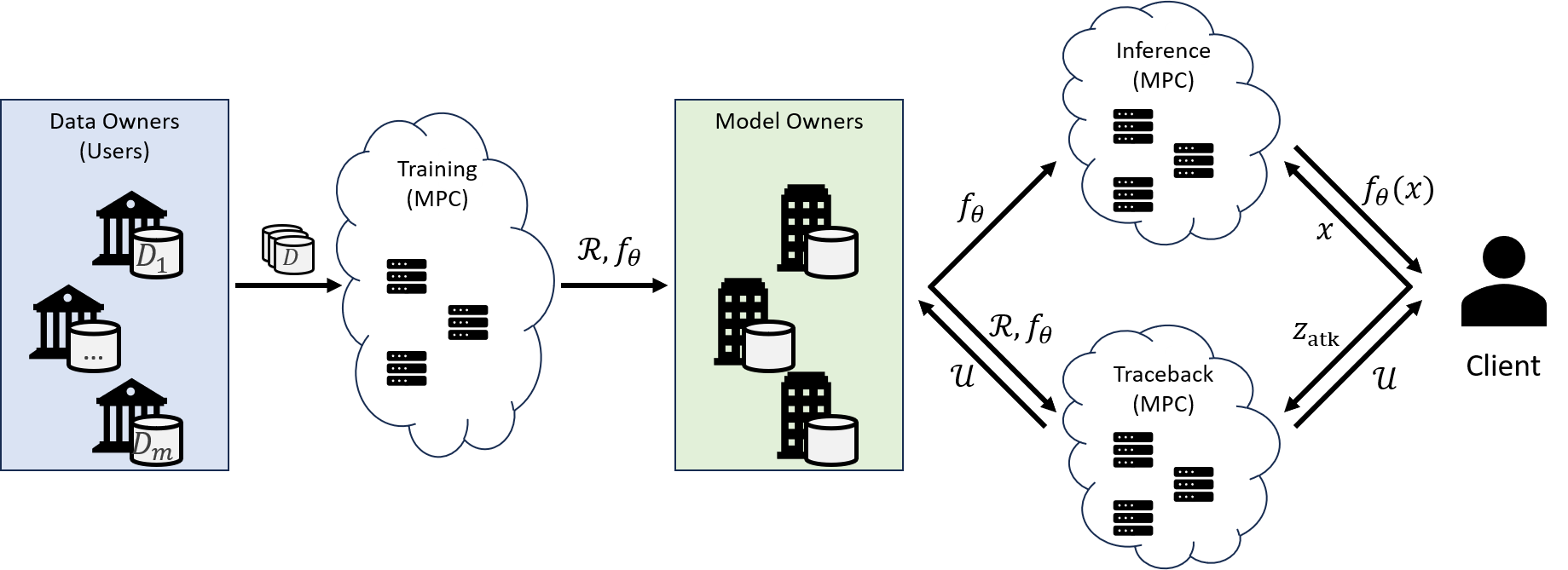
Figure 1: The considered PPML scenario includes data owners contributing their private datasets to train an ML model $f_{\theta}$ distributively in MPC. MPC servers are ephemeral and do not store long-term state. Model owners store model shares of $f_{\theta}$ and training records $R$ that are used for private inference. A traceback service monitors suspicious activity during model deployment and launches a procedure to identify malicious data owners $\mathcal{U}$ given a suspicious input $z_{\mathrm{atk}}$.

To create the service, the model owners negotiate with $m$ data owners $U_{1},\ldots,U_{m}$, each of whom owns a user dataset $D_{i}$ whose elements are labeled samples from the space $\mathcal{Z}=\mathcal{X}\times\mathcal{Y}$, where $\mathcal{X}$ is the $d$-dimensional feature space and $\mathcal{Y}$ is the discrete label set. The data owners lease their data to the model owners for the purpose of training a model $f_{\theta}$, without directly revealing their private datasets. Training is performed using MPC-based PPML to distribute trust among two or more parties [4, 74, 73, 95] who perform the necessary computations to produce the trained model $f_{\theta}$ on the joint dataset $D_{\mathrm{tr}}:=\bigcup_{i=1}^{m}D_{i}$. The resulting model $f_{\theta}$ is given to the model owners in a secret-shared format. Additionally, the training procedure generates a record $R$ of the training process (that might include model checkpoints, training hyperparameters, validation metrics, or other train-time artifacts), also secret shared to the model owners.

After training the model privately, a black-box inference service is provided to clients. Clients submit private queries $x\in\mathcal{X}$ to the service, which computes $\hat{y}=f_{\theta}(x)$ using a secure MPC inference procedure and returns the predicted output.

User-level poisoning traceback. The novel component we add to a PPML service is a secure traceback service. The ML training algorithm might implement poisoning defenses, such as [19, 92, 94, 42], but we envision the traceback service to provide another layer of defense. As a deployment-level service, poisoning traceback complements existing defenses by allowing system maintainers to address attacks that evade defenses. A main requirement is that the traceback service is attack agnostic and generalizes to multiple attack strategies.

The traceback service receives misclassification events from clients at deployment time. The service’s goal is to analyze the attack events and training record $R$ to identify compromised data owners responsible for poisoning. We perform traceback with a single misclassification event, as in prior traceback work [88, 70, 40]. The traceback service needs to also identify any false positives, such as mis-classification events that are due to normal ML errors and not data poisoning. The traceback procedure outputs for the model owners a ranking of all users based on raw responsibility scores, and a list of accused users identified as malicious, typically by setting a threshold on the responsibility scores.

We focus on user-level poisoning traceback, in contrast to most prior work performing sample-level traceback [88], that is, identifying training samples responsible for the attack event. In PPML, an important requirement is maintaining data privacy, and revealing sample-level scores might enable violations such as membership inference attacks [62].

3.2 Threat Model

We consider an actively malicious adversary that can compromise parties across the training, inference, and traceback phases. The adversary can observe and modify all inputs, states and network traffic of the compromised parties. We assume the adversary controls a minority of each group of data owners, model owners, and computational parties.

For the compromised data owners, we assume that the adversary controls their training datasets to mount a data poisoning attack on the ML model. We consider an error-specific misclassification objective [11], that is, inducing a specific prediction $f_{\theta}(x)=\hat{y}\neq y$, where $\hat{y}$ is a target label and $y$ is the true label for the point $x$. This objective can be achieved through a number of methods, including backdoor attacks [21, 38, 91, 84, 79, 14] and label-flipping attacks [49]. In terms of adversarial knowledge, we assume the strongest white-box adversary with full knowledge of the training algorithm, the traceback mechanism, and training datasets of compromised clients.

For the compromised servers in the inference and traceback MPC protocols, we consider standard adversarial models from PPML. Typically, the adversary controls a minority of servers in the computation, but the exact threshold depends on the PPML protocol. Certain instantiations of secure computation might impose additional constraints on the adversary. For example, our system can be used with MPC protocols that assume an honest-but-curious adversary that only passively corrupts the parties [8, 16], which are frequently significantly more efficient than their actively secure counterparts that consider malicious adversaries [95, 27].

We assume that clients submitting mis-classification events to the traceback service are not acting maliciously. Indeed, malicious clients might submit arbitrary events to the traceback service to mount a denial-of-service attack or intentionally incriminate a data owner. Existing work provides secure mechanisms for addressing these issues, via cryptographic commitments [71], that can be added to our system to help defend against malicious clients.

3.3 Design Goals and Challenges

A traceback tool in PPML should fulfill the following design requirements, which present certain inherent challenges:

High effectiveness. The traceback tool should identify malicious users with high precision and low false positive rates. False accusations can lead to legal consequences for innocent data owners; therefore, we focus on maximizing true positive rate (TPR) at low false positive rates (FPR). This is challenging to achieve as stealthy poisoning attacks require control of less than 1% of the training set [87, 86].

Generality across attacks. Existing poisoning defenses often make assumptions on either the nature of the poisoning attack [94, 97, 77, 101], clean data distribution [23, 22, 31, 61], or learning algorithm [92, 83, 60, 45]. These assumptions are necessary for defining anomalous behavior at training-time. Instead, we have the ambitious goal to design deployment-level traceback tools that generalize across attacks.

Handle coordinated poisoning attacks. Adversaries may spread poisoned data across multiple user datasets to make their behavior appear less suspicious and evade detection. A resilient traceback framework must handle such coordinated attacks, and this requirement has been identified as a prominent challenge by prior work [70].

Maintain privacy. The traceback tool should maintain the privacy of users’ datasets. This requirement precludes trivial adaptations of sample-level traceback methods that compute and release scores for all samples in a user’s dataset.

Low storage overhead. Reliance on training data for traceback is impractical because data owners might be unavailable at deployment time. Additionally, data owners may be required by external factors (e.g., privacy laws) to delete certain sensitive information after leasing it for model training [37, 30, 12]. The secure ML service must maintain additional records for traceback and minimize the storage overhead for these records.

Low performance overhead. In line with MPC protocol design requirements, we seek to minimize the runtime of the traceback protocol and the number of communication rounds, which should scale efficiently with the number of data owners $m$ and the size of user datasets $|D_{i}|$.

4 UTrace Framework

In this section, we construct our framework for performing user-level poisoning traceback. We start by describing several existing techniques for poisoning traceback, and mention their limitations. We then introduce our gradient-similarity method that creates user-level responsibility scores by identifying and aggregating the most relevant samples in the user’s dataset. We discuss various insights and optimizations to arrive to a complete traceback method that addresses the design requirements from Section 3.3.

4.1 Adapting Prior Techniques

To motivate the design of our traceback framework, we examine the techniques used in recent work on poisoning traceback and evaluate their suitability for PPML.

Poison Forensics. Poison Forensics (PF) [88] is a sample-level traceback method that identifies benign points by clustering candidate poisons in gradient space. Each cluster is “approximately unlearned” by applying first-order updates to the model using a custom objective. If unlearning a cluster does not affect the model’s behavior on the attack sample, it is regarded as benign and removed from the poison set. This process repeats until no more points can be removed.

Adapting clustering-based traceback procedures to private learning is challenging. Due to the privacy requirements imposed by MPC, each clustering round must process the entire training dataset to avoid privacy leakage. This computation is expensive and cannot be easily amortized as a preprocessing step.

Cryptographic auditing. Camel [70] is the only existing approach for user-level traceback in PPML. For each user, Camel computes updated model parameters by unlearning that user’s dataset and checking if the misclassification event is corrected. This method works well for a single malicious data owner, but is not as effective when the attacker distributes poisons across several user datasets.

We highlight some limitations of unlearning-based traceback in Appendix A. We observe that the approximate unlearning objective used by PF and Camel differs significantly from true unlearning, which can be exploited by an attacker. We also show that, in an idealized learning setting, using true unlearning with models trained with empirical risk minimization fails catastrophically if poisons are duplicated across even two user datasets (see Figure 5).

Gradient Similarity. A recent line of work in ML has developed explainability methods to attribute model behavior to training data [41, 33, 78, 51]. [78] defines a sample-level influence metric that measures the impact of individual training points on model predictions. Their method, TracInCP, defines training data influence as a weighted sum of gradient inner products over the parameter trajectory taken during training. Hammoudeh et al. [40] extend TracInCP by introducing Gradient Aggregated Similarity (GAS), which replaces inner product with cosine similarity.

Gradient similarity methods can be viewed as a type of counterfactual analysis: If the model $\theta$ is trained on data point $z$, in what direction does the loss on test point $\hat{z}$ move? This connects to a basic assumption we make about the malicious nature of poisoning attacks – that benign points do not have sufficiently high gradient alignment to decrease the loss on the attack sample, and thus poisoned points must induce gradients with higher alignment in order to manipulate the model’s behavior. This assumption is exceedingly general, making gradient-based scores appropriate as a general-purpose influence measure that does not rely on additional assumptions about attack strategy.

Importantly for our application to collaborative learning, for some fixed model parameters $\theta$, the gradient similarity score assigned to each training point does not depend on the multiplicity of the training point in the training set. This stands in stark contrast to unlearning-based methods, where the influence of a point (or group of points) implicitly depends on whether other copies of the point remain in the training set after unlearning. This property is crucial in handling poisoning distributed over several user datasets.

The remaining obstacles with respect to challenges from Section 3.3 are effectiveness at low poisoning rates and the absence of user data during traceback. Intuitively, at low poisoning rates, the poisons are required to be more effective: hence, we expect poisons to appear even more suspicious, as measured by gradient similarity. Moreover, a useful property of gradient-based influence scores is that they only depends on gradient inner products. If gradients are cached during training, they can be used during traceback without relying on the presence of training data.

4.2 Extending Gradients to Users

Building on our insights, gradient-based influence scores appear the most promising for implementing poisoning traceback in PPML. The main challenge is how to adapt gradient similarity techniques to operate at the user level. We begin by recalling the GAS score [40]. Before training, an iteration set $\mathcal{T}\subseteq[T]$ is fixed, where $T$ is the number of training steps. Typically $|\mathcal{T}|\ll T$. During training, at iterations $t\in\mathcal{T}$, the intermediate model parameters $\theta_{t}$ are recorded along with the current learning rate $\eta_{t}$. The sample-level influence score $\mathcal{I}_{\cos}$ between training point $z$ and test point $\hat{z}$ is then defined as

$$\mathcal{I}_{\cos}(z,\hat{z})=\sum_{t\in\mathcal{T}}\eta_{t}\frac{\left\langle\nabla_{\theta}\ell(\theta_{t};z),\,\nabla_{\theta}\ell(\theta_{t};\hat{z})\right\rangle}{\lVert\nabla_{\theta}\ell(\theta_{t};z)\rVert_{2}\lVert\nabla_{\theta}\ell(\theta_{t};\hat{z})\rVert_{2}}.$$ (1)

To extend this score to the user level, we aim to directly leverage the natural partitioning of the training set into user datasets along with the assumption that fewer than 50% of user datasets are malicious. Our approach is to define a user-level responsibility score, and then to compare these scores across users to identify disproportionately responsible users.

There are two main approaches one could consider here. The first is to treat sample-level influence score as a black box and aggregate these scores into an influence score for each user. A simple way to achieve this is to compute the influence score for each sample in a user’s dataset, and then to define the user influence score by aggregating the sample scores within a user’s dataset. Second, we could attempt to directly modify the similarity-based influence metric to accommodate sets of training points rather than individual data points.

Motivated by our discussion, we define two user-level event responsibility metrics based on weighted sums of gradient similarities, which we call $\mathcal{I}_{\cos}^{\mathrm{s}}$ and $\mathcal{I}_{\cos}^{\mathrm{p}}$. For a dataset $D$ and model parameters $\theta$, let $\mathcal{L}(\theta;D)=\sum_{z\in D}\ell(\theta;z)$. Given a training record $R$ consisting of model checkpoints $\theta_{t}$ and learning rates $\eta_{t}$, we define the $\mathcal{I}_{\cos}^{\mathrm{s}}$ and $\mathcal{I}_{\cos}^{\mathrm{p}}$ influence scores between a user’s dataset $D_{i}$ and test point $\hat{z}$ to be

$$\mathcal{I}_{\cos}^{\mathrm{s}}(D_{i},\hat{z},R)$$

$$\quad:=\frac{1}{|D_{i}|}\sum_{z\in D_{i}}\sum_{t\in\mathcal{T}}\eta_{t}\frac{\left\langle\nabla_{\theta}\ell(\theta_{t};z),\,\nabla_{\theta}\ell(\theta_{t};\hat{z})\right\rangle}{\lVert\nabla_{\theta}\ell(\theta_{t};z)\rVert_{2}\lVert\nabla_{\theta}\ell(\theta_{t};\hat{z})\rVert_{2}}$$

$$\quad=\frac{1}{|D_{i}|}\sum_{z\in D_{i}}\mathcal{I}_{\cos}(z,\hat{z})$$ (2)

$$\mathcal{I}_{\cos}^{\mathrm{p}}(D_{i},\hat{z},R)$$

$$\quad:=\sum_{t\in\mathcal{T}}\eta_{t}\frac{\left\langle\nabla_{\theta}\mathcal{L}(\theta_{t};D_{i}),\,\nabla_{\theta}\ell(\theta_{t};\hat{z})\right\rangle}{\lVert\nabla_{\theta}\mathcal{L}(\theta_{t};D_{i})\rVert_{2}\lVert\nabla_{\theta}\ell(\theta_{t};\hat{z})\rVert_{2}}$$ (3)

Restated, $\mathcal{I}_{\cos}^{\mathrm{s}}$ is a weighted sum of the mean sample-level gradient cosine similarity with $\hat{z}$, taken over the samples of $D_{i}$. In contrast, $\mathcal{I}_{\cos}^{\mathrm{p}}$ is a weighted sum over dataset-level gradients computed using $D_{i}$. Note that the two definitions do not coincide in general.

4.3 Effective Scoring Function

Both scores $\mathcal{I}_{\cos}^{\mathrm{s}}$ and $\mathcal{I}_{\cos}^{\mathrm{p}}$ assume that the gradient signal from the poisoned data is strong enough to outweigh contributions from other data points in the adversarial user dataset $D_{i}$. However, when poisoning occurs at exceptionally low poisoning rates (e.g., 0.1% of user data), the relevant terms become diluted and fail to indicate malicious behavior. To address this challenge, our influence score should primarily target the malicious portions of a corrupted dataset.

Top-$k$ selection. Our main insight is to identify the most influential samples within each user’s data and include them in the aggregated user score. As $\mathcal{I}_{\cos}^{\mathrm{s}}$ aggregates GAS scores across samples, we propose to identify first the top-k samples with highest GAS scores and then aggregate only scores for those samples. If we define:

$$S_{i}=\{\mathcal{I}_{\cos}^{\mathrm{s}}(z,\hat{z}):z\in D_{i}\}$$ (4)

then the user responsibility score is:

$$s_{i}=\tfrac{1}{k}\sum_{j=1}^{k}\mathrm{top\text{-}}k(S_{i})_{j}$$ (5)

where $\mathrm{top\text{-}}k(S_{i})$ is a multiset containing the largest $k$ elements of $S_{i}$. Note that determining the most influential samples for $\mathcal{I}_{\cos}^{\mathrm{p}}$ is not immediate and we will not consider this aggregation method further.

Considerations for choosing $k$. The hyperparameter $k$ determines the sensitivity of the traceback tool to low poisoning rates. At $k=1$, user scores are determined according to the single most suspicious data point in a user’s dataset. As $k$ grows large, the reduction method approaches $\mathcal{I}_{\cos}^{\mathrm{s}}$. In general, appropriate choices for $k$ depend on the learning task and network architecture.

4.4 Cost Effective Gradient Computation

Since training and traceback occur at different times, any inputs required for traceback must either be cached during training or re-supplied at traceback time. In particular, the gradients used in influence score computations can either be computed once during the training procedure and cached for future traceback executions, or recomputed during each traceback execution. Reusing cached gradients reduces runtime and removes the need for data owners to re-share private inputs during traceback. This is especially important in privacy-critical settings where data owners may be required to delete sensitive data when certain conditions are met [1].

Computing and storing sample-level gradients present two problems. First, computing full parameter gradients at each checkpoint can be expensive, since each checkpoint necessitates a forward and backward pass over the entire training set. Second, the long-term storage of sample-level gradients demands an untenable volume of storage space: the required storage grows linearly with the number of checkpoints $|\mathcal{T}|$, the training set size $|D_{\mathrm{tr}}|$, and the dimension of the model $\dim(\Theta)$. To improve the traceback efficiency, we introduce two strategies focused on gradient computation and storage.

Utilizing Final Layer Gradients. Prior work has observed that under common initialization and layer normalization techniques, the final layer is responsible for most of the gradient norm variation [54, 40]. Moreover, when computing gradients with the backpropagation algorithm, a layer’s gradient does not depend on earlier layers. By using gradients from only the model’s later layers, the cost of gradient computation is reduced to essentially that of a single forward pass. We find that using gradients from the final one or two layers of the network generally results in a marginal reduction in traceback effectiveness while significantly improving runtime.

Writing the network’s classification function as

$$f_{\theta}(x)=\mathrm{softmax}(\psi_{\theta_{\psi}}(\varphi_{\theta_{\varphi}}(x)))$$

for $\theta=[\theta_{\varphi}\enskip\theta_{\psi}]$ for parameterized feature extractor $\varphi$ and classification layers $\psi$, we replace all gradients $\nabla_{\theta}$ in a given gradient similarity score with $\nabla_{\theta_{\psi}}$. The resulting influence score can be interpreted as the mean gradient alignment at given classification parameters over a sequence of feature extractors.

Gradient Projection and Caching. A popular technique for data-oblivious dimensionality reduction is to use random projections to form low-dimensional sketches [53, 99]. Recently, Pruthi et al. showed how to use sketches to reduce the storage requirements for training data gradients in gradient-based influence methods [78]. The idea is to apply a random projection into a low-dimensional vector space in a way which approximately preserves inner products. The projection dimension is controlled by the model trainer and can be chosen according to the desired trade-off between long-term storage constraints and future traceback performance.

We perform random gradient projection by choosing a random matrix $G\in\mathbb{R}^{r\times p}$, where $r$ is the desired projection dimension and $p$ is the native gradient dimension, where $\mathbb{E}[G^{T}G]=I_{p}$. The result induces an unbiased (over the randomness of $G$) estimator of the inner product between any two (fixed) vectors $u,v\in\mathbb{R}^{p}$:

$$\mathbb{E}[(Gu)^{T}(Gv)]=\mathbb{E}[u^{T}G^{T}Gv]=u^{T}v.$$

Following Pruthi et al., we sample $G$ by choosing its entries i.i.d. from $\mathcal{N}(0,1/r)$. Additionally, we consider a variation of Pruthi et al.’s gradient projection strategy. Instead of re-using the same projection matrix across all checkpoints, we propose to sample a new projection matrix at each checkpoint. We do this to reduce the probability of obtaining a single low-quality projection for a given downstream misclassification event, at the cost of additional storage space. Despite requiring storage of multiple projection matrices, the overhead does not grow with the number of training samples. Hence, for large enough datasets, using many low-dimensional projections consumes less storage space than using a single high-dimensional projection applied at all checkpoints.

Low-dimensional gradient sketches can be directly reused between traceback executions. Thus, we view the computation of projected gradients as a pre-processing step embedded inside the training procedure. At key checkpoints, the training algorithm generates projection matrices $G_{t}$ and projected gradients $g_{t}$ of the training loss. These projected gradients are then used for multiple downstream traceback computations.

4.5 Framework Details

The complete UTrace requires modifying the training loop in PPML and implementing the traceback method.

Training Routine. We describe the full UTrace training in Algorithm 1, incorporating all improvements discussed in Sections 4.3 and 4.4. The training output consists of both the trained model parameters $\theta_{t}$ and the training record $R$. Each element in $R$ contains the learning rate $\eta_{t}$, intermediate model parameters $\theta_{t-1}$, the training data gradients $g_{t}$, and the projection matrix $G_{t}$ for some training iteration $t\in\mathcal{T}$.

Algorithm 1 Training Procedure

1:Training dataset $D_{\mathrm{tr}}$, checkpoint set $\mathcal{T}$, iteration count $T$, learning rate schedule $\eta_{0},\ldots,\eta_{T}$, initial parameters $\theta_{0}$, gradient projection dimension $d$

2:Trained model parameters $\theta_{T}$, training record $R$

3:$R\leftarrow\emptyset$

4:for $t\leftarrow 1$ to $T$ do

5:     if $t\in\mathcal{T}$ then

6:         $G_{t}\leftarrow\textsc{RandomProjection}(n,d)$

7:         $\mathbf{g_{t}}\leftarrow\mathbf{0}$

8:         for $i\leftarrow 1$ to $|D_{\mathrm{tr}}|$ do

9:              $x_{i},y_{i}\leftarrow D_{\mathrm{tr}}[i]$

10:              $g_{t}^{(i)}\leftarrow G_{t}\,\nabla_{\theta_{W}}\ell(\theta_{t-1};x_{i},y_{i})$

11:         end for

12:         $R\leftarrow R\cup\{(\eta_{t},\theta_{t-1},g_{t},G_{t})\}$

13:     end if

14:     $\theta_{t}\leftarrow\textsc{Step}(\theta_{t-1},\eta_{t},D_{\mathrm{tr}})$

15:end for

16:return $(\theta_{T},R)$

Traceback Routine. We describe the UTrace traceback procedure in Algorithm 2. Given a misclassification event $z_{\mathrm{atk}}$, traceback computes user responsibility scores and outputs a ranked list of users based on these scores.

Algorithm 2 User-level Traceback Procedure

1:User datasets $D_{1},\ldots,D_{m}$, Misclassification event $z_{\mathrm{atk}}$, Training record $R=\{(\theta_{t-1},\eta_{t},g_{t},G_{t})\}_{t\in\mathcal{T}}$, Score parameter $k$

2:Ranked owners by responsibility scores $\mathcal{U}$

3:// Pre-compute projected traceback gradients

4:for $t\in\mathcal{T}$ do

5:     $\widehat{g_{t}}\leftarrow G_{t}\nabla_{\theta_{W}}\mathcal{L}(\theta_{t-1};z_{\mathrm{atk}})$ // $G_{t},\theta_{t-1}$ from $R$

6:end for

7:for $i=1,\ldots,m$ do

8:     $I_{i}\leftarrow\textsc{Indices}(i)$ // User $i$’s indices

9:     $S_{i}\leftarrow\left\{\sum_{t\in\mathcal{T}}\eta_{t}\frac{\left\langle g_{t}^{(\mathrm{idx})},\,\widehat{g_{t}}\right\rangle}{\left\lVert g_{t}^{(\mathrm{idx})}\right\rVert_{2}\left\lVert\widehat{g_{t}}\right\rVert_{2}}:\text{idx}\in I_{i}\right\}$

10:     $s_{i}\leftarrow\frac{1}{k}\sum_{j=1}^{k}\mathrm{top\text{-}}k(S_{i})_{j}$

11:end for

12:return $\textsc{RankUsers}(\widetilde{s_{1}},\ldots,\widetilde{s_{m}})$

4.6 Secure UTrace

We now discuss the secure UTrace protocol that realizes the traceback algorithm in the MPC setting. Achieving traceback in secure computation involves overcoming several challenges related to both the oblivious nature of secure computation and scalability. We construct our protocol from several cryptographic primitives, including ideal functionalities to abstract PPML protocols for ML training and inference. Due to space constraints, we formally describe the functionalities mentioned in this work in Section B.1. By $[\![\,\cdot\,]\!]$, we denote a secret-shared value, and we sometimes abuse this notation for secret-shared vectors and matrices.

The main overhead of realizing Algorithm 2 as $\Pi_{\mathsf{\text{UTrace}}}$ (c.f. Protocol 3) comes from the gradient computation, computing the cosine distance between the gradients, and finding the $\mathrm{top\text{-}}k$ samples. The gradient computation is model-dependent and similar to training, so in the following we focus on realizing latter two computations efficiently. For the cosine similarity, a challenge is fixed-point division and approximating the divisor’s square roots. Integer division and square root operations require significantly more communication rounds compared to other operations, increasing both latency and bandwidth usage. Prior work proposed protocols for integer division and square roots by relying on Goldschmidt and Raphson-Newton iterations [6]. However, we can rewrite the gradient magnitudes in the divisor as a single square root operation due to the commutativity of multiplication with the square root for positive numbers.

$$\begin{split}\frac{\left\langle g_{t}^{(\mathrm{idx})},\,\widehat{g_{t}}\right\rangle}{\left\lVert g_{t}^{(\mathrm{idx})}\right\rVert_{2}\left\lVert\widehat{g_{t}}\right\rVert_{2}}=\frac{\left\langle g_{t}^{(\mathrm{idx})},\,\widehat{g_{t}}\right\rangle}{\sqrt{\sum_{i}(g_{t,i}^{(\mathrm{idx})})^{2}\cdot\sum_{i}(\widehat{g_{t,i}})^{2}}}\end{split}$$

This allows us to compute the cosine distance using a single reciprocal square root of the squared gradient magnitudes. The reciprocal square root appears in various deep learning primitives such as softmax, batch normalization, and optimizers such as Adam and AMSGrad and efficient approximation protocols exist [66, 56].

After computing the cosine distances, we select the $\mathrm{top\text{-}}k$ from a list of $d$ distance scores. Standard techniques to compute $\mathrm{top\text{-}}k$, such as using a $k$-sized min-heap, are challenging to apply efficiently to the secure setting, because of the requirement for the computation to be oblivious. Although there exists prior work on data-oblivious algorithms for $\mathrm{top\text{-}}k$ based on merging networks[25], we found that sorting and selecting the first $k$ samples to be efficient for MPC. This is due to the efficiency of the oblivious sorting algorithm, which relies on random permutations in order to achieve a round complexity independent of the number of samples [39].

Heuristic Sample Selection. Although the previous optimization of multiplying by the reciprocal square root improves efficiency, we still have to compute $\mathcal{O}(|\mathcal{T}|\cdot|D_{i}|)$ reciprocals per partition for each traceback. Therefore, we propose another optimization to improve the computational complexity of the $\mathrm{top\text{-}}k$ cosine score selection. The key idea is to leverage the fact that $\mathrm{top\text{-}}k$ involves a sum over only $k$ terms. If those $k$ terms can be (approximately) identified without exactly computing the values over all training samples in a partition, we can compute expensive operations over only those samples. The full protocol is presented in Protocol 5 in Appendix B.2.

We propose a $\mathrm{top\text{-}}(k,l)$ selection scheme, in which a coarser set $\tilde{I}_{i}$ of $l$ indices are determined via a heuristic function $h(z,\hat{z})$, where $z$ is a training sample $z$ and $\hat{z}$ the test sample. The elements $\left\{D_{i}^{(j)}:\text{j}\in\tilde{I}_{i}\right\}$ are then used instead of $D_{i}$ for the subsequent scoring function. To compute $\tilde{I}_{i}$, we adapt the existing $\mathrm{top\text{-}}l$ procedure as $\mathrm{top\text{-}}k_{I}$ to return indices instead of scores directly.

$$\tilde{I}_{i}=\mathrm{top\text{-}}l\left(\left\{(j,h(D_{i}^{(j)},\hat{z})):j\in 1,\ldots,|I_{i}|\right\}\right)$$

We provide a full description of this extension in Algorithm 4 in Section B.2. We implement $h$ as the ranking induced by the un-normalized gradient scores [78]:

$$h(z,\hat{z})=\sum_{t\in\mathcal{T}}\eta_{t}\left\langle\nabla_{\theta}\ell(\theta_{t};z),\,\nabla_{\theta}\ell(\theta_{t};\hat{z})\right\rangle.$$ (6)

Our choice of $h$ is significantly faster than directly computing cosine scores for each sample because multiplications require fewer rounds of communication than divisions. Although this algorithm introduces an extra selection of the $\mathrm{top\text{-}}l$ samples in addition to $\mathrm{top\text{-}}k$, it is more efficient when $l\ll|D_{i}|$.

Realizing Selection in MPC. A challenge with realizing the heuristic in MPC is that the computation must be data-oblivious. In particular, the top-$l$ samples that we select with the heuristic cannot influence the subsequent computation, such as array accesses based on $\tilde{I}_{i}$. A naïve transformation to oblivious computation would entail doing the computation for all entries in $D_{i}$ and combining the result with an indicator bit based on whether we want to select the entry or not, but this removes the efficiency benefits of the algorithm, i.e., having to compute a cosine score for the full input array.

To overcome this issue, we extend the vector that is sorted for $\mathrm{top\text{-}}l_{I}$ to a matrix that includes the data required for computing the final score $\mathcal{I}_{\cos}^{\mathrm{s}}$. We compute $\mathcal{I}_{\cos}^{\mathrm{s}}$ as

$$\sum_{t\in\mathcal{T}}\eta_{t}\cdot\mathcal{F}_{\mathsf{fp-mul}}([\![\,\mathbf{d}^{(j)}_{t}\,]\!],\mathcal{F}_{\mathsf{fp-rsqrt}}([\![\,\text{N}^{(j)}_{t}\,]\!]))\text{ for }j\in[|\tilde{I}_{i}|].$$

where $[\![\,\mathbf{d}^{(j)}_{t}\,]\!]$ is the inner product between the two gradients $[\![\,\mathbf{d}^{(j)}_{t}\,]\!]$ and $[\![\,\text{N}^{(j)}_{t}\,]\!]$ is the product of the squared gradient magnitudes for each checkpoint $t$. We extend each row of the sort matrix $\mathsf{M}$ with $2\cdot|\mathcal{T}|$ columns to include $\left\{[\![\,\mathbf{d}^{(1)}_{t}\,]\!]\right\}_{t\in\mathcal{T}}$ and $\left\{[\![\,\text{N}^{(1)}_{t}\,]\!]\right\}_{t\in\mathcal{T}}$ as

$$\mathsf{M}=\begin{pmatrix}[\![\,\mathbf{d}^{(1)}\,]\!]&\left\{[\![\,\mathbf{d}^{(1)}_{t}\,]\!]\right\}_{t\in\mathcal{T}}&\left\{[\![\,\text{N}^{(1)}_{t}\,]\!]\right\}_{t\in\mathcal{T}}\\ [\![\,\mathbf{d}^{(2)}\,]\!]&\left\{[\![\,\mathbf{d}^{(2)}_{t}\,]\!]\right\}_{t\in\mathcal{T}}&\left\{[\![\,\text{N}^{(2)}_{t}\,]\!]\right\}_{t\in\mathcal{T}}\\ {3}\\ [\![\,\mathbf{d}^{(|I_{i}|)}\,]\!]&\left\{[\![\,\mathbf{d}^{(|I_{i}|)}_{t}\,]\!]\right\}_{t\in\mathcal{T}}&\left\{[\![\,\text{N}^{(|{I}_{i}|)}_{t}\,]\!]\right\}_{t\in\mathcal{T}}\end{pmatrix}$$

resulting in a $|{I}_{i}|\times(2|\mathcal{T}|+1)$-sized matrix that must be sorted. Sorting a matrix instead of a vector incurs some additional overhead in MPC. In particular, the radix-sorting algorithm used in our implementation incurs a linear communication overhead in the number of columns due to the shuffling sub-protocol, but no additional rounds [39].

We introduce another delayed truncation optimization in Appendix B.3.

5 Experimental Results

We test our traceback tool by training classifiers under a total of ten different poisoning attacks and four representative datasets from three modalities: vision, malware, and text.

5.1 Evaluation setup

We run UTrace on Ubuntu 24.04 machines with at least 128GB of memory and different GPU configurations including Nvidia RTX A6000, Nvidia TITAN X (Pascal), and Nvidia GeForce GTX TITAN X.

Datasets and models. We summarize the datasets and models we use in our experiments. Detailed training configurations, including hyperparameters, can be found in Appendix C.

CIFAR-10. CIFAR-10 [59] is a 10-class image dataset of 32x32 RGB images. We train image classifiers using ResNet-18 models [43]. CIFAR-10 is well-established as a poisoning benchmark and a wide suite of attacks work against it [5, 32, 91, 49, 85].

Fashion. Fashion MNIST [100] is a 10-class image dataset of 28x28 grayscale images. We train image classifiers using a small convolutional network.

EMBER. EMBER [7] is a malware classification dataset of 2351-dimensional examples with features extracted from Windows Portable Executable (PE) files. We train using the EmberNN architecture from Severi et al. [86].

SST-2. SST-2 [89] is a sentiment classification text dataset containing film reviews. SST-2 has been used in prior work [40] as a benchmark for sample-level poisoning traceback in the text domain.

Partitioning Data. We use 10 data owners that contribute their datasets to model training, but we also experiment with 20 owners, leading to similar results. To partition the datasets, we sample class labels from a Dirichlet distribution [46] $q\sim\text{Dir}(\alpha p)$, where $p$ is the prior label distribution. We set $\alpha=100$ for all of our experiments, which simulates a scenario with almost uniform distribution across owners. We vary the number of poisoned owners between 1 and 4, and distribute the poisoned samples randomly across the malicious owners.

Metrics. We measure both the effectiveness and efficiency of our traceback tool.

Our traceback tool supports two output configurations, producing either a ranking on all users or a list of accused users. We thus leverage two types of metrics for evaluating the effectiveness our system: ranking metrics and classification metrics. First, we model traceback as an information retrieval task and report the mean average precision (mAP) and mean reciprocal rank (mRR) scores for each attack scenario. These metrics measure if the malicious owners are ranked high among all owners according to their responsibility scores. In the second configuration, we need to determine a threshold on responsibility scores to generate a list of accused users. We train benign models and compute standardized influence scores for benign misclassifications events under different random samplings from the clean data distribution. Thresholds are chosen to correspond to a low false positive rate (0.1%) on these benign misclassifications. We report both the precision and recall for each attack under this threshold, as well as the global AUC metric.

We evaluate the efficiency of our system using three metrics: round complexity, communication complexity, and overall runtime. Round complexity measures the number of communication rounds needed in the MPC protocol. Communication complexity measures the total data exchanged. Overall runtime captures the total execution time, including training and traceback, in both LAN and WAN settings.

Traceback parameters. We report influence metric hyperparameters for unlearning and our method in Table 6 in Section C.1. In general, we sample checkpoints at some uniform interval until reaching a maximum checkpoint set size. We choose unlearning parameters using reasonable fine-tuning settings for each learning task.

5.2 Existing Poisoning Attacks on Vision

We begin our evaluation with standard attacks against CIFAR-10 and Fashion datasets. For space, we present detailed results for only CIFAR-10 here, and defer detailed Fashion results to Section D.2. Our qualitative findings are similar between both datasets.

Attack setup. We evaluate our tool against four different poisoning attacks: two backdoor attacks (BadNets [38] and Sleeper Agent [91]), Subpopulation [49], and targeted (Witches’ Brew [32]). BadNets and Subpopulation attacks are dirty-label attacks: the attacker has control over data labeling and can insert mislabeled points. Witches’ Brew and Sleeper Agent are clean-label attacks which work by applying small perturbations to inputs without changing their labels. Clean-label attacks are generally much more difficult to detect because they blend into the clean data distribution. We give complete details on attack setup in Section C.2.

Results. We report the ranking metrics for attacks against CIFAR-10 / ResNet-18 in Table 1 and the classification metrics in Table 2. We also plot attack-conditioned ROC curves in Figure 2.

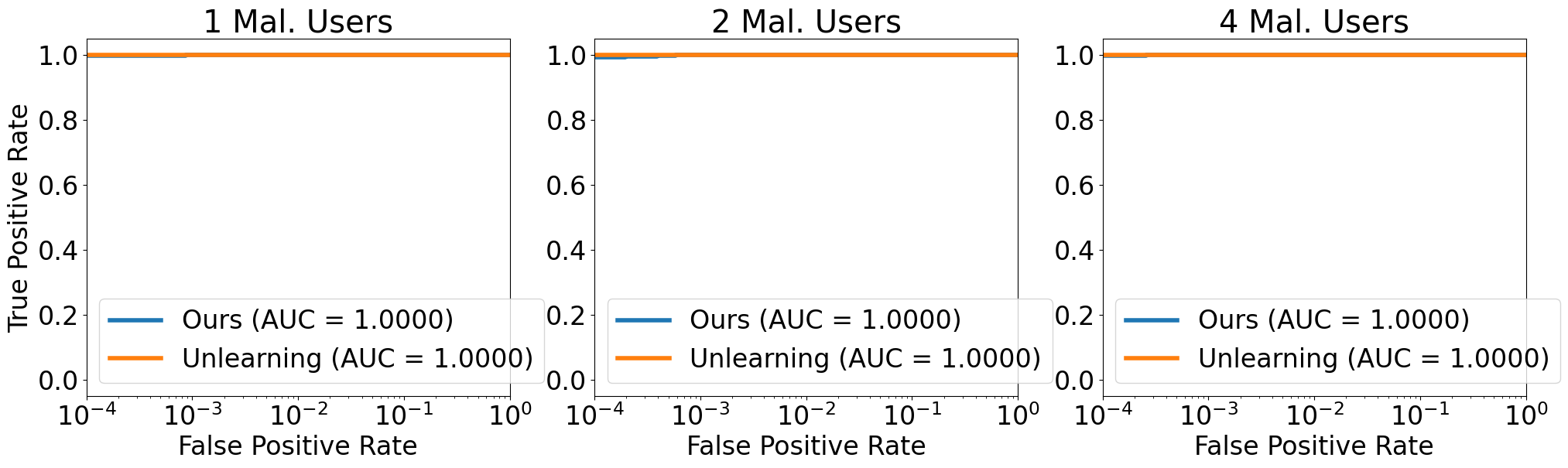
(a) BadNets

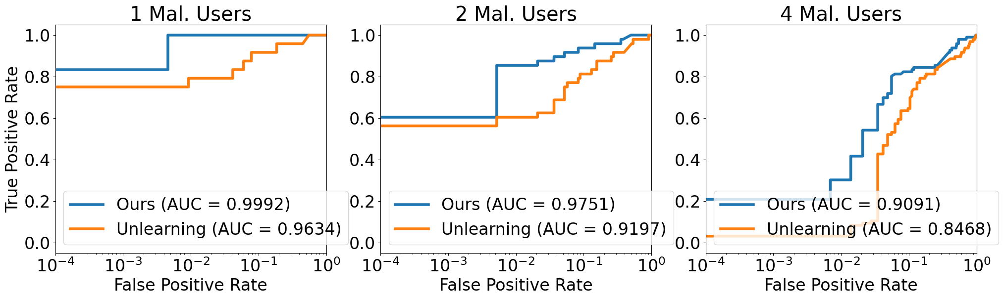
(b) Witches’ Brew

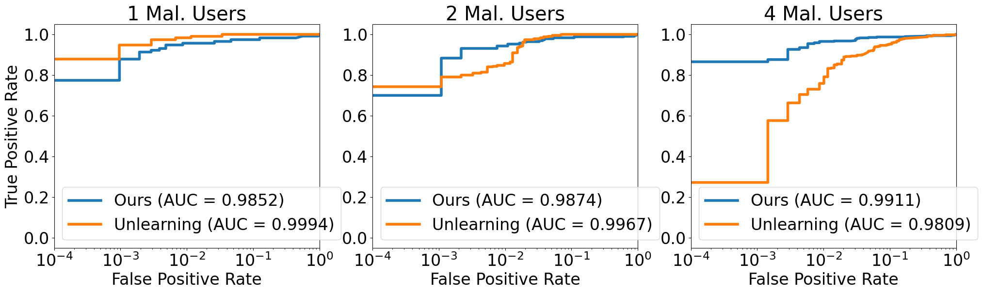
(c) Subpopulation

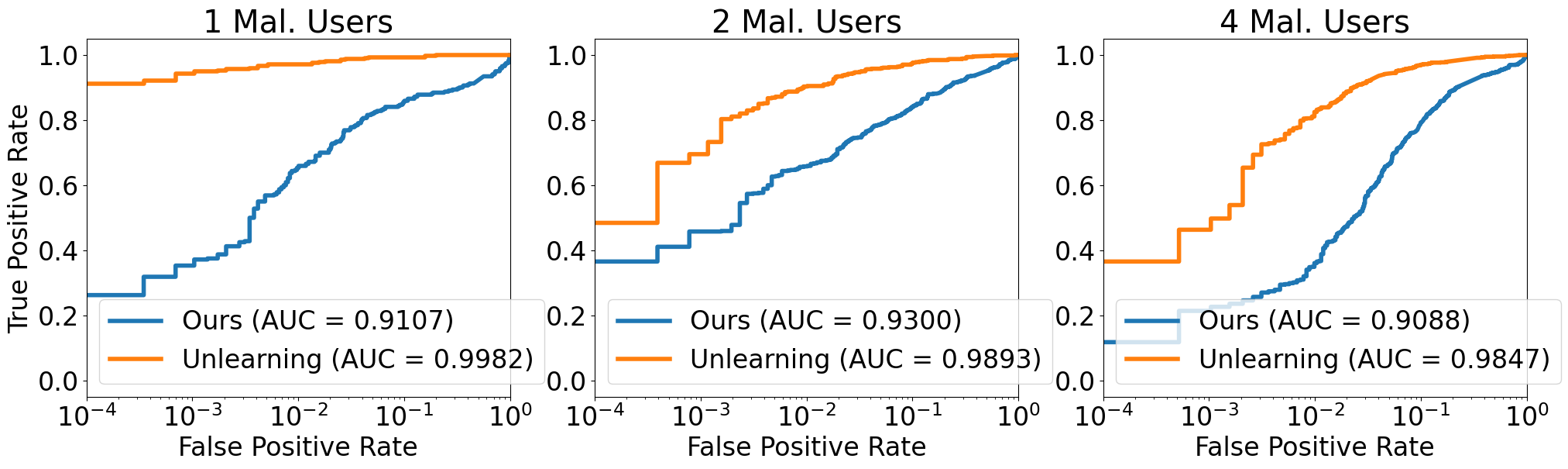
(d) Sleeper Agent

Figure 2: Malicious user identification ROC curves for standard attacks against CIFAR-10 / ResNet18.

Table 1: Ranking metrics (mAP and mRR) for standard attacks against CIFAR-10 / ResNet18. Highest score is bold if the two methods are not identical.

Attack	Mal. Users	Unlearning		Ours
		mAP	mRR	mAP	mRR
BadNets	1	1.0000	1.0000	1.0000	1.0000
	2	1.0000	1.0000	1.0000	1.0000
	3	1.0000	1.0000	1.0000	1.0000
	4	1.0000	1.0000	1.0000	1.0000
Witch	1	0.9132	0.9132	1.0000	1.0000
	2	0.8740	0.8958	0.9736	1.0000
	3	0.8433	0.9181	0.9543	1.0000
	4	0.8404	0.9028	0.9103	1.0000
Subpop	1	1.0000	1.0000	0.9823	0.9823
	2	1.0000	1.0000	0.9839	0.9853
	3	0.9883	0.9921	0.9855	0.9907
	4	0.9763	0.9921	0.9878	0.9940
Sleeper	1	0.9958	0.9958	0.8885	0.8885
	2	0.9837	0.9918	0.8971	0.9045
	3	0.9840	0.9870	0.8978	0.9224
	4	0.9807	0.9953	0.8975	0.9207

Table 2: Classification metrics for standard attacks against CIFAR-10 / ResNet18 at 0.1% FPR.

Attack	Mal. Users	Unlearning		Ours
		TPR	FPR	TPR	FPR
BadNets	1	1.0000	0.0247	0.9984	0.0002
	2	1.0000	0.0152	0.9937	0.0000
	3	1.0000	0.0071	0.9896	0.0000
	4	1.0000	0.0023	0.9547	0.0000
Witch	1	0.2500	0.0000	0.5000	0.0000
	2	0.0833	0.0000	0.1875	0.0000
	3	0.0139	0.0000	0.0139	0.0000
	4	0.0000	0.0000	0.0000	0.0000
Subpop	1	0.9206	0.0009	0.7222	0.0000
	2	0.5476	0.0000	0.6349	0.0000
	3	0.1984	0.0000	0.4709	0.0000
	4	0.0159	0.0000	0.2401	0.0000
Sleeper	1	0.7937	0.0000	0.3531	0.0010
	2	0.4719	0.0000	0.2609	0.0000
	3	0.2313	0.0000	0.1604	0.0000
	4	0.0938	0.0000	0.0016	0.0000

For BadNets, UTrace consistently achieves over 95% TPR with a maximum FPR of just 0.02%, outperforming unlearning-based scores, which show a FPR exceeding 2%. The higher FPR under unlearning can be attributed to the use of a loss-based influence score. At a poisoning rate of 5%, backdoor samples have much lower loss than typical samples. When unlearning benign datasets, the loss on an attack sample can range over several orders of magnitude. This variation makes unlearning prone to benign outliers due to larger loss variability at small scales. However, our gradient-based responsibility scores can reliability detect multiple compromised data owners with very low FPR.

In Subpopulation attacks, UTrace’s effectiveness remains stable, while unlearning declines with more poisoned owners. Specifically, unlearning’s mAP drops from 0.991 with one poisoned dataset to 0.9763 with four. In contrast, our method stays above 0.9823. The classification metrics also reflect this finding, with unlearning dropping to a TPR of 1.59% compared to our method’s 24.01% under four poisoned owners.

The clean-label poisoning attacks Witches’ Brew and Sleeper Agent prove more challenging for both traceback tools, due to the stealthy nature of both attacks. For Witches’ Brew, UTrace outperforms unlearning across all metrics, achieving mRR scores of 1.0 in all settings, versus a mRR of $\leq$ 0.92 for unlearning. For Sleeper Agent, UTrace underperforms unlearning by getting a mAP score of $\geq$ 0.8885 compared to 0.98 by unlearning. The TPR at low FPR values are low for both tools.

Parameter ablations. We vary the value of $k$ for the top-$k$ metric for different attacks. We find that setting $k$ too small ($k<16$ for CIFAR-10) weakens performance as the poisoning samples might not be included in the user score. On the other hand, if $k$ is too large, the benign samples influence the score more than poisoned samples. The value of $k=32$ provides good results for several attacks.

We run UTrace with 20 owners to evaluate the impact of the number of users. On BadNets, our method’s effectiveness deteriorates slightly, while unlearning maintains strong ranking. On Subpopulation attacks, our method improves from the 10 user setting, reaching $\geq 0.6$ TPR with 8 poisoned owners. Conversely, Unlearning degrades to a TPR of 0. Full results are in Section D.1.

Summary. Our results indicate that gradient-based influence scores can consistently identify responsible data owners with high success. In most cases (i.e., all attacks except Sleeper Agent), UTrace outperforms unlearning in both ranking and classification metrics. UTrace is also more resilient as the number of poisoned owners increases and has lower FPR than unlearning.

5.3 Attacks against Unlearning

Attack setup. Motivated by our analysis in Appendix A, we implement two poisoning adversaries that prove challenging for unlearning. The first “Noisy BadNets” attack adds large amounts of label noise to backdoor samples with the goal of inducing a nearly uniform posterior distribution in the victim classifier on attack samples.

The second adversary is based on the observation that approximate unlearning scores rely on high attack success rates when unlearning clean datasets. Moreover, applying the unlearning objective to clean data can degrade the model’s performance on the clean data distribution. By tying the attack’s success to the model’s accuracy on clean data, we can make clean datasets appear suspicious and thereby weaken the approximate unlearning responsibility metric. We achieve this by implementing a “permutation” backdoor: the attack chooses a derangement $\sigma\colon C\to C$ and aims to misclassify samples from each class $i$ as class $\sigma(i)\neq i$. We indicate permutation BadNets with “$\sigma$-BadNets” and annotate label noise variants accordingly.

Results. We report the ranking metrics for these attacks against CIFAR-10 / ResNet-18 in Table 3 and the classification metrics in Table 4. We also plot ROC curves in Figure 3.

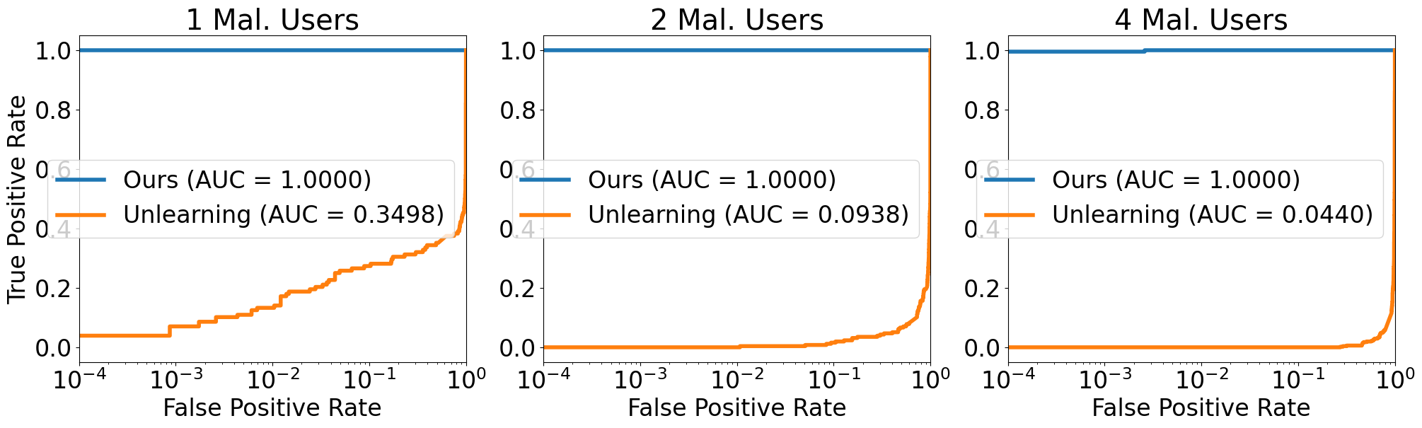
(a) Noisy BadNets

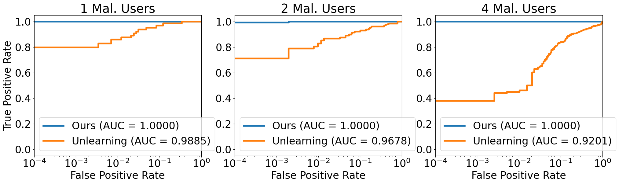
(b) $\sigma$-BadNets

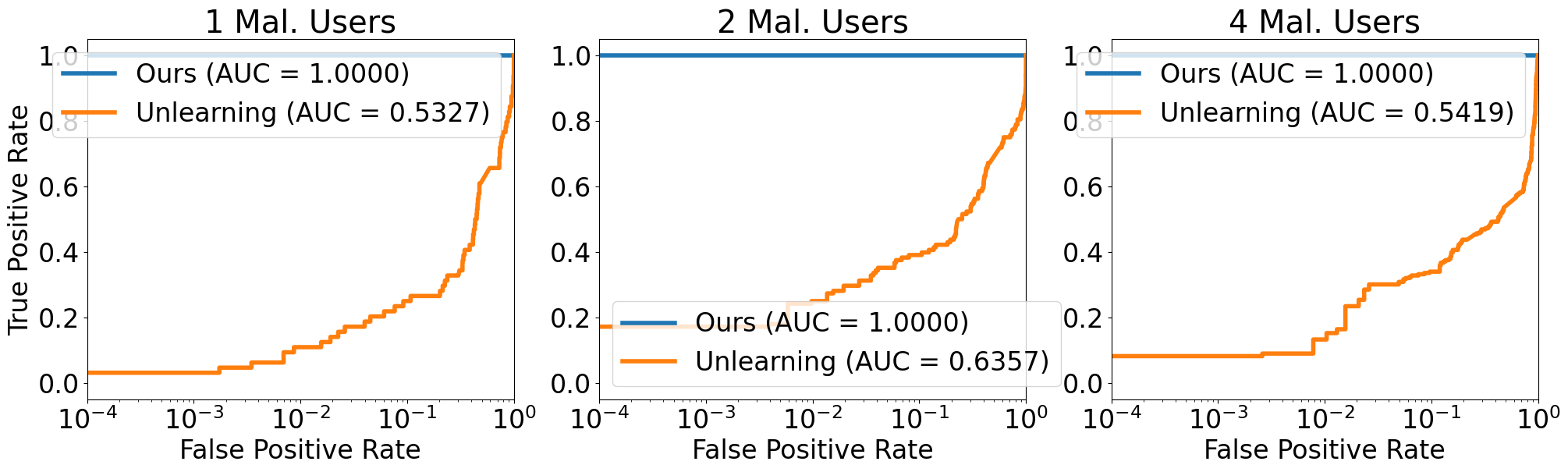
(c) Noisy $\sigma$-BadNets

Figure 3: Malicious user identification ROC curves for unlearning-aware attacks against CIFAR-10 / ResNet18.

Table 3: mAP and mRR scores for unlearning-aware attacks against CIFAR-10 / ResNet18. Highest score is bold if the two methods are not identical.

Attack	Mal. Users	Unlearning		Ours
		mAP	mRR	mAP	mRR
Noisy BadNets	1	0.6519	0.6519	0.9976	0.9976
	2	0.4844	0.5859	0.9979	0.9985
	3	0.5209	0.6324	0.9983	0.9991
	4	0.5352	0.6266	0.9981	0.9983
$\sigma$-BadNets	1	0.9733	0.9733	1.0000	1.0000
	2	0.9485	0.9584	1.0000	1.0000
	3	0.9278	0.9509	1.0000	1.0000
	4	0.9170	0.9507	1.0000	1.0000
Noisy $\sigma$-BadNets	1	0.3151	0.3151	1.0000	1.0000
	2	0.4123	0.5117	1.0000	1.0000
	3	0.4608	0.5633	0.9998	1.0000
	4	0.5310	0.6764	0.9996	1.0000

Table 4: Classification metrics for unlearning-aware attacks against CIFAR-10 / ResNet18 at 0.1% FPR.

Attack	Mal. Users	Unlearning		Ours
		TPR	FPR	TPR	FPR
Noisy BadNets	1	0.2205	0.0002	0.9948	0.0006
	2	0.0556	0.0004	0.9922	0.0000
	3	0.0156	0.0000	0.9878	0.0000
	4	0.0000	0.0000	0.9531	0.0000
$\sigma$-BadNets	1	0.7891	0.0011	1.0000	0.0015
	2	0.5840	0.0005	0.9971	0.0005
	3	0.3822	0.0000	0.9681	0.0000
	4	0.1865	0.0000	0.7827	0.0000
Noisy $\sigma$-BadNets	1	0.0059	0.0002	0.9980	0.0002
	2	0.0127	0.0002	0.9932	0.0005
	3	0.0156	0.0000	0.9811	0.0000
	4	0.0024	0.0000	0.8999	0.0000

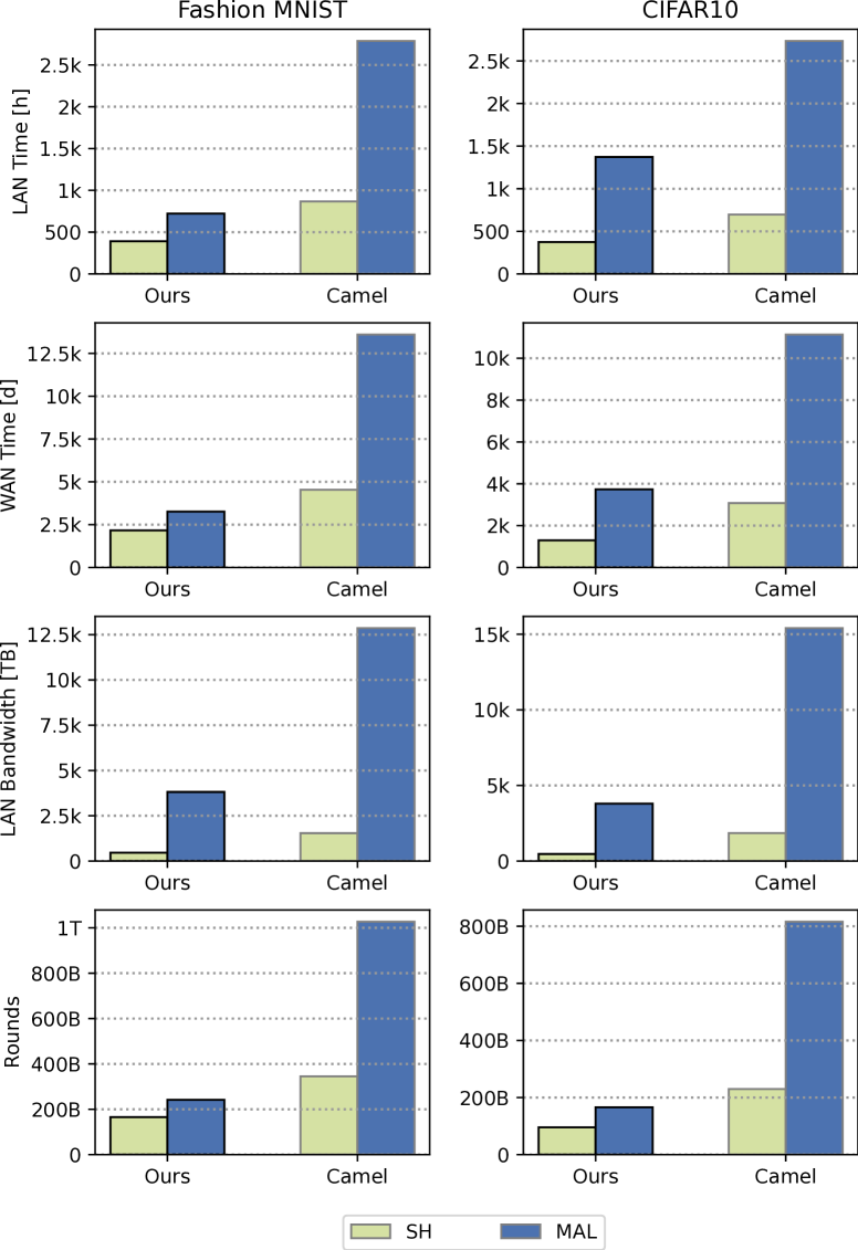
(a) Preprocessing

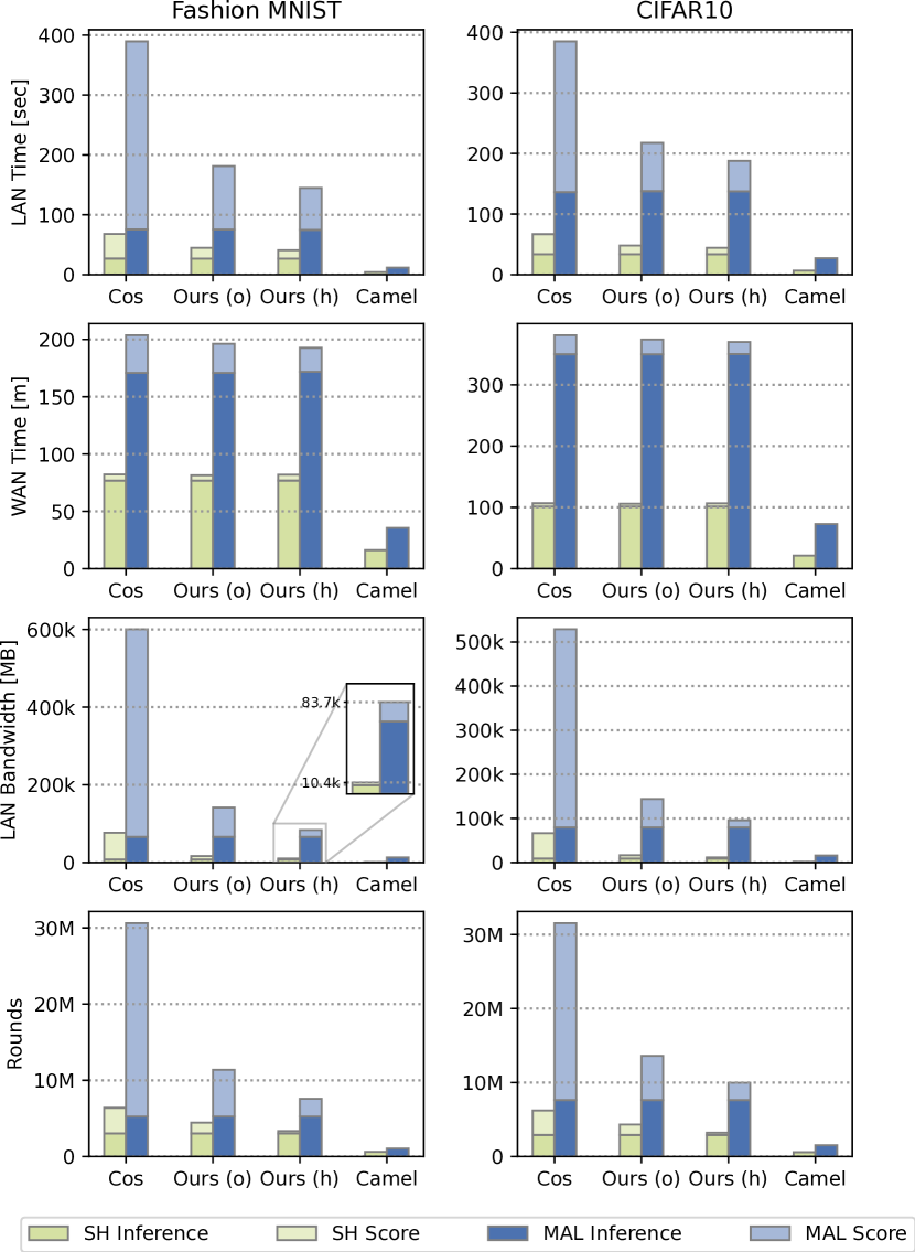
(b) Online

Figure 4: Evaluation of Secure UTrace compared to Camel. Ours (o) refers to the version of UTrace with the reciprocal square root optimization, and Ours (h) refers to UTrace with the heuristic sample selection.

Adding label noise to the poisons significantly impacts the influence scores computed by approximate unlearning. Unlearning attains a mAP as low as 0.4844 and a mRR as low as 0.5859, reached under two poisoned owners. In contrast, UTrace achieves mAP and mRR above 0.99.

The permutation backdoor drops unlearning effectiveness from a mAP of 0.973 with one poisoned dataset to 0.917 with four poisoned datasets. This contrasts with the consistent mAP of 1.0 with the one-to-one backdoor objective. The classification metrics show similar degradation, with a drop in TPR from 78.9% with one poisoned dataset to 18.7% with four. In contrast, UTrace maintains high TPR of 100% and 78.2% with one and four poisoned owners, respectively.

Combining both strategies, the noisy $\sigma$-BadNets causes the most severe degradation in approximate unlearning effectiveness. With just one poisoned dataset, approximate unlearning achieves a mAP score of only 0.3151, while UTrace has mAP $\geq$ 0.999 and mRR of 1 even for four poisoned owners.

Summary. Our results highlight a serious weakness of the approximate unlearning method. The attacks we designed are general and can potentially apply to other attack objectives and poisoning strategies as well. We showed that UTrace maintains robust ranking and classification metrics for all these attack variants.

5.4 Text and Malware Experiments

We present the results for experiments against the SST-2 and Ember datasets in Section D.3 and summarize the findings here. First, we find that the inner-product heuristic does not select relevant poisoning samples in the text modality. Hence, we use full $\mathrm{top\text{-}}k$ selection for attacks against SST-2. We experiment with four types of backdoor attack against SST-2 and two backdoor attacks against Ember. In general, we find the same trend of degradation in approximate unlearning as the number of poisoned datasets increases. For example, under a “style” text backdoor [76] against SST-2, our method achieves a TPR of 81.25%, versus the unlearning TPR of 4.7%. A similar result follows for an explanation-guided backdoor attack against Ember [86], where our method achieves a TPR of 98.4% versus the unlearning TPR of 5.9%.

5.5 Secure UTrace

We now evaluate the performance of UTrace in MPC. Our implementation is based on MP-SPDZ [55], a popular framework for MPC computation that supports a variety of protocols. We also compare UTrace with Camel [70], the only existing poisoning traceback tool in MPC.

Experimental Setup. We run UTrace on AWS c5.9xlarge machines running Ubuntu 20.04, each equipped with 36 vCPUs of an Intel Xeon 3.6 Ghz processor and 72 GB of RAM. The machines are connected over a local area network (LAN) through a 12 Gbps network interface with an average round-trip time (RTT) of $0.5$ ms. We additionally perform our experiments in a simulated wide area network (WAN) setting using the tc utility to introduce an RTT of $80$ ms and limit the bandwidth to $2$ Gbps. We report the total wall clock time and the communication cost based on the data sent by each party, which includes the time and bandwidth required for setting up any cryptographic material for the MPC protocol, such as correlated randomness. As both our algorithm and Camel contain parts that can be reused across computations, we split the cost into preprocessing and online phases.

Preprocessing. We first compare the preprocessing performance of UTrace with Camel. UTrace’s preprocessing entails computing and compressing the gradients of the training dataset $D$ for all model checkpoints in $\mathcal{T}$, resulting in $O(|D|\cdot|\mathcal{T}|)$ gradient computations. Camel approximately unlearns $m$ leave-one-out models, taking $O(|D|\cdot m\cdot e)$ forward and backward passes for $e$ unlearning epochs. In addition, because UTrace only requires the gradient of the final layers in the model, the gradient computation obviates the need for a full backward pass, unlike Camel’s training procedure.

The wall-clock time and bandwidth results shown in Figure 4(a) highlight this improvement. Roughly speaking, for Camel, the additional $m\cdot e$ training epochs is similar to performing a full training run, taking 696 hours and 2734 hours for semi-honest and malicious protocols, respectively, for CIFAR-10 in the LAN setting. UTrace’s overhead shows an $2-3.5$x reduction over Camel’s, taking only 374 hours and 1372 hours for semi-honest and malicious protocols, respectively. In conclusion, the cost of the traceback procedure is only a fraction of the MPC training cost.

Online. We compare the wall-clock time and bandwidth costs of the online time of the strawman, the optimization and the heuristic versions of UTrace, as well as Camel in Figure 4(b). The overhead of Camel is 27 seconds for the malicious protocol in LAN and 73 minutes in WAN for CIFAR-10, because it only requires $O(m)$ forward passes of the test sample, i.e., one inference per input party. UTrace, on the other hand, requires $O(|\mathcal{T}|)$ forward passes in order to compute the gradients for each checkpoint, which take 137 seconds for the malicious protocol in LAN and 350 minutes in WAN. The reason for Camel’s faster latency is that the number of parties $m$ is smaller than the number of checkpoints $|\mathcal{T}|$ in our setting.

In addition to the inference, computing cosine distances introduces an additional overhead of $1.8-4.2$x (an extra $249-314$ seconds) in the malicious LAN setting. We reduce this overhead to $0.58-1.41$x in LAN using the reciprocal square root optimization. UTrace with the heuristic optimization further reduces this overhead to $0.36-0.94$x of the forward pass cost. In absolute terms, the cost of doing a traceback is 44-48 seconds (105-106 minutes) and 187-217 seconds (370-374 minutes), respectively, for the semi-honest and malicious protocols in the LAN (WAN) setting for CIFAR-10. Considering the cost of a single inference in the LAN (WAN) setting, 0.83 and 2.25 seconds (2 and 6.8 minutes), the overhead of running UTrace is reasonable. Note that these numbers include the cost to compute input-independent cryptographic material of the underlying MPC protocols, and MPC-protocol-dependent preprocessing optimizations can be applied to reduce latency further.

6 Conclusions, Limitations, and Future Work

We design a user-level traceback procedure UTrace in PPML with high effectiveness and low FPR that generalizes across backdoor, targeted, and subpopulation attacks. Compared to unlearning-based methods such as Camel [70], UTrace achieves higher TPR at low FPR, and provides a better ranking of malicious users. Our optimizations make the tool practical in PPML settings, as the pre-processing cost is $2-3.5$x lower than that of Camel, at the cost of a slight increase in online traceback cost.

Both UTrace and Camel are less successful at identifying malicious users for the clean-label Sleeper Agent and Witches’ Brew attacks. These attacks use low poisoning rates, and are generated subject to strict perturbation constraints relative to the training samples, making them more difficult to differentiate from legitimate data. The combination of clean-label threat model and high variance in attack success rate make these attacks a challenging setting for traceback. Methods for traceback that achieve higher effectiveness might require additional misclassification events, or more information about the attack category.

Since the attack sample is not known at training time, the iteration set $\mathcal{T}$ must be selected without knowledge of which checkpoints capture the attack behavior most. Our tool computes user responsibility scores using the selected checkpoints, and relies on the learning of the attack behavior by these model checkpoints. Currently, we sample checkpoints uniformly spaced over training, but this might not be the best strategy. If the attack behavior is learned too late into the training loop, or if the attack behavior is learned too quickly by the model, our sampling strategy might be suboptimal. Developing more effective checkpointing methods may require some insight into the nature of the attack, which we leave as a topic for future work.

Finally, we discuss interesting directions for future work on adaptive attacks against our system. Our method assumes poisoned samples exhibit alignment with an adversarial objective represented by the attack sample. This assumption holds for all the attacks considered in this paper. However, it may be possible to construct attacks that violate this requirement: for example, in neural networks it may be possible for poisons to induce behavior in the the network’s feature extractor which is indirectly related to the poisoning objective. Demonstrating the existence of such attacks would have widespread implications.

Appendix A Analysis of Unlearning

In this section, we examine unlearning-based traceback from a theoretical perspective to understand in what scenarios it can be expected to detect poisoning.

In Section A.1, We examine the basic assumptions made by approximate unlearning, and discuss scenarios where they fail. We pair these findings with experimental results demonstrating the failure modes with concrete attacks. These results demonstrate that there exist attacks, some natural and some adaptive, which evade detection by approximate unlearning, motivating the need for better responsibility scores.

In Section A.2, we state and prove a theorem characterizing a failure mode of true unlearning for user-level detection; that is, in the case when the approximate unlearning routine $\operatorname{Unl}(\theta;D^{\prime};D_{\mathrm{tr}})$ is replaced with retraining from-scratch on the dataset $D^{\prime}\setminus D_{\mathrm{tr}}$. This result implies that the vulnerabilities of approximate unlearning cannot be resolved simply by resorting to a more accurate unlearning procedure. In fact, approximate unlearning provides resilience to multiple poisoned owners.

A.1 Approximate Unlearning Failure Modes

Approximate unlearning is a heuristic technique for unlearning user datasets, and lacks formal guarantees about the resulting classifier. In this section, we analyze the properties of the approximate unlearning objective more carefully and do not assume the unlearned classifier necessarily behaves like a leave-one-out model. We show that by understanding what assumptions approximate unlearning makes, we can discover and explore scenarios where it fails.

Distributional Analysis. To make analysis tractable, we remove the learning aspect and consider a distributional setting. Let $\mu_{c}$ and $\mu_{p}$ be distributions over $\mathcal{Z}=\mathcal{X}\times\mathcal{Y}$, representing the clean and poisoned data distributions, respectively. Let $\alpha\in(0,1)$ be the mixture weights between $\mu_{c}$ and $\mu_{p}$, so that the poisoned training distribution is the mixture $\alpha\mu_{c}+(1-\alpha)\mu_{p}.$ Additionally, let $0<\beta<\min(\alpha,1-\alpha)$ be the unlearning fraction representing the fraction of samples to be unlearned. For simplicity, we assume that this weight is equal for both $\mu_{c}$ and $\mu_{p}$, which is analogous to the assumption that poisoned and clean user datasets all have the same size. Specifically, we define the approximately unlearned distributions

$$\nu^{\mathrm{unl}}_{p} =\alpha\mu_{c}+\beta\mu_{p}^{\mathrm{unl}}+(1-\alpha-\beta)\mu_{p}$$ (7)

$$\nu^{\mathrm{unl}}_{c} =(\alpha-\beta)\mu_{c}+\beta\mu_{c}^{\mathrm{unl}}+(1-\alpha)\mu_{p},$$ (8)

where $\mu_{p}^{\mathrm{unl}}$ and $\mu_{c}^{\mathrm{unl}}$ represent the poisoned and clean distributions with labels replaced by a uniform posterior, respectively.

Our goal is to understand the behavior of $\nu^{\mathrm{unl}}_{p}(y^{\mathrm{atk}}|x^{\mathrm{atk}})$ and $\nu^{\mathrm{unl}}_{c}(y^{\mathrm{atk}}|x^{\mathrm{atk}})$ for some attack sample $(x^{\mathrm{atk}},y^{\mathrm{atk}})\in\mathcal{Z}$. In particular, these quantities are the related to the loss-based influence score used by approximate unlearning. If these quantities are sufficiently close to each other, the unlearning-based score will be less reliable as an indicator of poisoning. We begin by stating a useful fact describing the input-conditioned label posterior for general mixtures:

Lemma A.1.

Let $\mu_{1},\ldots,\mu_{n}$ be distributions over $\mathcal{Z}$, and let $0<\alpha_{1},\ldots,\alpha_{n}<1$ be mixing weights (i.e., $\sum_{i}\alpha_{i}=1$). Let $\nu=\sum_{i}\alpha_{i}\mu_{i}$. Then, for all $(x,y)\in\mathcal{Z}$,

$$\nu(y|x)=\sum_{i=1}^{n}\lambda_{i}\mu_{i}(y|x)$$ (9)

where

$$\lambda_{i}=\frac{\alpha_{i}\mu_{i}(x)}{\sum_{j=1}^{n}\alpha_{j}\mu_{j}(x)}.$$ (10)

Lemma A.1 is a straightforward consequence of Bayes’ Theorem, and describes the posterior $\nu(y|x)$ as a convex combination of posteriors $\mu_{1}(y|x),\ldots,\mu_{n}(y|x)$. In particular, the posteriors under both $\nu^{\mathrm{unl}}_{p}$ and $\nu^{\mathrm{unl}}_{c}$ are given by

$$\nu^{\mathrm{unl}}_{p}(y|x)$$

$$=\frac{\alpha\mu_{c}(x)\mu_{c}(y|x)+\tfrac{\beta}{C}\mu_{p}(x)+(1-\alpha-\beta)\mu_{p}(x)\mu_{p}(y|x)}{\alpha\mu_{c}(x)+(1-\alpha)\mu_{p}(x)}$$ (11)

$$\nu^{\mathrm{unl}}_{c}(y|x)$$

$$=\frac{(\alpha-\beta)\mu_{c}(x)\mu_{c}(y|x)+\tfrac{\beta}{C}\mu_{c}(x)+(1-\alpha)\mu_{p}(x)\mu_{p}(y|x)}{\alpha\mu_{c}(x)+(1-\alpha)\mu_{p}(x)}$$ (12)

where $C$ is the number of classes. We can inspect Equations 11 and 12 for certain representative poisoning settings. For instance, for classification tasks with unambiguous labeling, it is likely that $\mu_{c}(y^{\mathrm{atk}}|x^{\mathrm{atk}})=0$, and so the posteriors simplify to

$$\nu^{\mathrm{unl}}_{p}(y|x) =\frac{\tfrac{\beta}{C}\mu_{p}(x)+(1-\alpha-\beta)\mu_{p}(x)\mu_{p}(y|x)}{\alpha\mu_{c}(x)+(1-\alpha)\mu_{p}(x)}$$

$$\nu^{\mathrm{unl}}_{c}(y|x) =\frac{\tfrac{\beta}{C}\mu_{c}(x)+(1-\alpha)\mu_{p}(x)\mu_{p}(y|x)}{\alpha\mu_{c}(x)+(1-\alpha)\mu_{p}(x)}.$$

For backdoor attacks, it is additionally possible that $\mu_{c}(x)=0$ if the trigger does not appear in benign samples. In this case, we obtain the more succinct characterization

$$\nu^{\mathrm{unl}}_{p}(y|x) =\mu_{p}(y|x)+\frac{\beta}{1-\alpha}(1/C-\mu_{p}(y|x))$$

$$\nu^{\mathrm{unl}}_{c}(y|x) =\mu_{p}(y|x).$$

The above relations suggest two conditions under which the loss-based influence score might fail to distinguish between benign and poisoned distributions: first, if the ratio $\beta/(1-\alpha)$ is small (that is, if too few poisons are unlearned), and second, if the poisoned posterior $\mu_{p}(y|x)$ is sufficiently close to uniform. Note that in the first case, if $\mu_{p}(y|x)$ is large (near 1), then even a small decrease in the posterior from unlearning can correspond to a large loss difference. We believe this contributes to the success of approximate unlearning in detecting backdoor attacks, even in cases where poisons are distributed across multiple poisoned datasets. On the other hand, when $\mu_{p}(y|x)$ is nearly uniform, the differences in loss are less extreme.

A.2 True Unlearning Failure Modes

Given the deficiencies of approximate unlearning demonstrated in Section A.1, it may seem tempting to replace it with an unlearning mechanism which more accurately approximates leave-one-out retraining. However, we show that in fact true unlearning exacerbates the ability of the adversary to hide poisons among multiple poisoned parties.

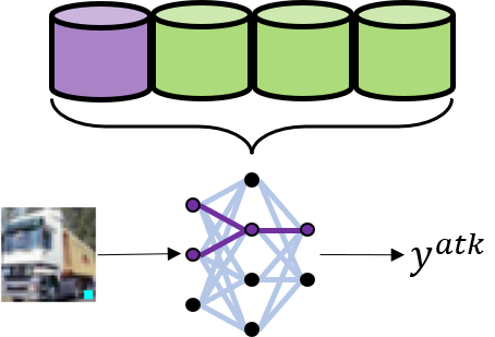
(a)

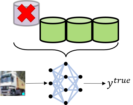
(b)

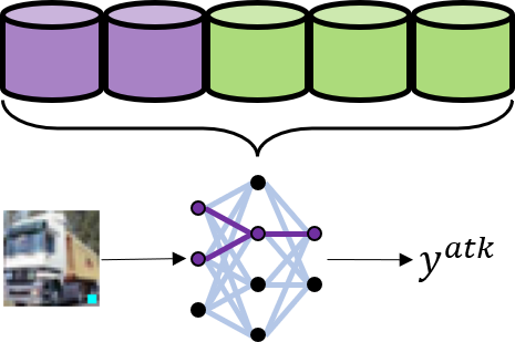
(c)

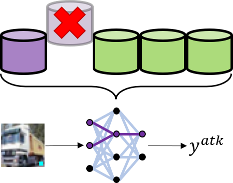
(d)

Figure 5: Different attack scenarios with concentrated versus distributed poisoning. (5(a)) A single user dataset contains poisons, causing a malicious classification. (5(b)) Retraining the model after removing the malicious dataset removes the malicious behavior from the model. (5(c)) Multiple user datasets contain poisons, causing a malicious misclassification. (5(d)). Removing only one of many poisoned datasets does not remove the malicious behavior from the retrained model.

In the case when the auditor produces the unlearned models $\theta_{i}^{\prime}$ by retraining from scratch for each user $i$, each time leaving out the user dataset $D_{i}$, the effect of duplicated poisons across multiple user datasets is exacerbated. We consider a minimal theoretical example demonstrating this possibility. Consider two distributions $\mu_{c}$ and $\mu_{p}$ over $\mathcal{X}\times\mathcal{Y}$, representing the clean and poisoned distributions, respectively. If the distributions $\mu_{c}$ and $\mu_{p}$ are compatible with each other, and if the model space $\Theta$ is sufficiently rich to simultaneously learn both distributions, then learning on any nontrivial mixture of those distributions yields the same set of loss-minimizing classifiers. Intuition for this idea is given Figure 5. We formalize this idea below:

Theorem A.2.

Let $\mu_{c}$ and $\mu_{p}$ be distributions over $\mathcal{Z}=\mathcal{X}\times\mathcal{Y}$, and let $\Theta\subseteq\mathbb{R}^{d}$ be a parameter space. For a nonnegative loss function $\mathcal{L}(\theta;\mu)=\mathbb{E}_{(x,y)\sim\mu}[\ell(\theta;x,y)]$, denote

$$\Theta_{c} :=\operatorname*{arg\,min}_{\theta\in\Theta}\mathcal{L}(\theta;\mu_{c})\subseteq\Theta$$

$$\Theta_{p} :=\operatorname*{arg\,min}_{\theta\in\Theta}\mathcal{L}(\theta;\mu_{p})\subseteq\Theta.$$

If $\Theta_{c}\cap\Theta_{p}\neq\emptyset$, then for all $\alpha\in(0,1)$, it holds that

$$\operatorname*{arg\,min}_{\theta\in\Theta}\mathcal{L}(\theta;\alpha\mu_{c}+(1-\alpha)\mu_{p})=\Theta_{c}\cap\Theta_{p}.$$

Proof.

Fix $\alpha\in(0,1)$. For notational convenience, denote

$$\nu:=\alpha\mu_{c}+(1-\alpha)\mu_{p}.$$

Additionally, denote by $L_{c}$ and $L_{c}$ the minimum loss achieved by those classifiers in $\Theta_{c}$ and $\Theta_{p}$, respectively.

We show inclusions on both sides. For all $\theta^{\prime}\in\Theta$, the mixture loss can be decomposed as

$$\mathcal{L}(\theta^{\prime};\nu)=\alpha\mathcal{L}(\theta^{\prime};\mu_{c})+(1-\alpha)\mathcal{L}(\theta^{\prime};\mu_{p}).$$ (13)

Since $\mathcal{L}(\theta;\mu_{c})\geq L_{c}$ and $\mathcal{L}(\theta;\mu_{p})\geq L_{p}$ by definition, we also have for all $\theta^{\prime}\in\Theta$ that

$$\mathcal{L}(\theta^{\prime};\nu)\geq\alpha L_{c}+(1-\alpha)L_{p}.$$ (14)

Moreover, since $\Theta_{c}\cap\Theta_{p}\neq\emptyset$, this is in fact the minimum attainable loss on $\nu$, attained by at least those classifiers in $\Theta_{c}\cap\Theta_{p}$. That is, we have shown the inclusion

$$\operatorname*{arg\,min}_{\theta\in\Theta}\mathcal{L}(\theta;\nu)\supseteq\Theta_{c}\cap\Theta_{p}.$$

Now, Suppose $\theta\in\operatorname*{arg\,min}_{\theta\in\Theta}\mathcal{L}(\theta;\nu)$. We must show that $\theta$ simultaneously minimizes loss on $\mu_{c}$ and $\mu_{p}$. Consider the case for $\mu_{c}$. We have shown that

$$\alpha\mathcal{L}(\theta;\mu_{c})+(1-\alpha)\mathcal{L}(\theta;\mu_{p})=\alpha L_{c}+(1-\alpha)L_{p}.$$

Rearranging, we find that

$$\mathcal{L}(\theta;\mu_{c}) =\tfrac{1}{\alpha}\left[\alpha L_{c}+(1-\alpha)(L_{p}-\mathcal{L}(\theta;\mu_{p}))\right]$$

$$\leq L_{c}.$$

Since $L_{c}$ minimizes loss on $\mu_{c}$, it follows that $\theta\in\Theta_{c}$. Symmetric argument shows that $\theta\in\Theta_{p}$, and thus

$$\operatorname*{arg\,min}_{\theta\in\Theta}\mathcal{L}(\theta;\nu)\subseteq\Theta_{c}\cap\Theta_{p}.$$ ∎

Implications of Theorem A.2. The distributions $\mu_{c}$ and $\mu_{p}$ in Theorem A.2 can be replaced with the empirical distributions $D_{i}$ for each user. Interpreted this way, the theorem describes a simplified setting where each user dataset is one of two possible datasets, $D_{c}$ or $D_{p}$. If the necessary assumptions are satisfied, performing true unlearning on any individual dataset that is duplicated across multiple users corresponds to setting a different $\alpha\in(0,1)$ (namely, $\alpha=\frac{a-1}{a+b-1}$, where $a$ and $b$ are the multiplicities of each dataset and we have removed one from those counted by $a$).

The condition that $\Theta_{c}\cap\Theta_{p}\neq 0$ requires that the learning tasks imposed by $\mu_{c}$ and $\mu_{p}$ are sufficiently compatible with each other, relative to the parameter space $\Theta$. This can be the case, for example, in backdoor attacks, where the supports of poisoned and clean distributions projected to the input space have trivial intersection (e.g., if no clean inputs contain the trigger). In this case, a sufficiently complex model can distinguish from which mixture an input originated and change its decision accordingly. The relationship between model complexity and backdoor susceptibility has been explored in recent work [72].

Appendix B Additional Details on Secure UTrace

B.1 Ideal Functionalities

In this appendix, we describe the ideal functionalities $\mathcal{F}_{\mathsf{fp-mul}}$, $\mathcal{F}_{\mathsf{mul}}$, $\mathcal{F}_{\mathsf{trunc}}$, $\mathcal{F}_{\mathsf{sort}}$, $\mathcal{F}_{\mathsf{gradient}}$, and $\mathcal{F}_{\mathsf{fp-rsqrt}}$, referenced in Protocols 3 and 5.

B.2 Secure UTrace Protocols

We present the UTrace protocol in Protocol 3. We also provide an algorithmic description of the heuristic version of UTrace in Algorithm 4, and the corresponding secure protocol in Protocol 5.

Protocol 3 $\Pi_{\mathsf{\text{UTrace}}}$

1:User datasets $[\![\,D_{1}\,]\!],\ldots,[\![\,D_{m}\,]\!]$, Misclassification event $z_{\mathrm{atk}}$, Training record $[\![\,R\,]\!]=\{([\![\,\theta_{t-1}\,]\!],\eta_{t},[\![\,g_{t}\,]\!],[\![\,G_{t}\,]\!])\}_{t\in\mathcal{T}}$, Score parameters $k,l$

2:Ranked owners by responsibility scores $\{i:U_{i}\}$

3:for $t\in\mathcal{T}$ do

4:     Run $[\![\,\widehat{g_{t}}\,]\!]\leftarrow\mathcal{F}_{\mathsf{gradient}}([\![\,G_{t}\,]\!],[\![\,\theta_{t-1}\,]\!],[\![\,z_{\mathrm{atk}}\,]\!])$

5:end for

6:for $i=1,\ldots,m$ do

7:     $I_{i}\leftarrow\textsc{Indices}(i)$ // User $i$’s indices

8:     for $t\in\mathcal{T}$ do

9:         Run $[\![\,\text{B}_{t}\,]\!]\leftarrow\mathcal{F}_{\mathsf{fp-dotp}}(\widehat{g_{t}},\widehat{g_{t}})$

10:         for $j=1,\ldots,|I_{i}|$ do

11:              Run $[\![\,\mathbf{d}^{(j)}_{t}\,]\!]\leftarrow\mathcal{F}_{\mathsf{fp-dotp}}([\![\,g_{t}^{(I_{i}^{(j)})}\,]\!],[\![\,\widehat{g_{t}}\,]\!])$

12:              Run $[\![\,\text{A}^{(j)}_{t}\,]\!]\leftarrow\mathcal{F}_{\mathsf{fp-dotp}}([\![\,g_{t}^{\mathrm{(I_{i}^{(j)})}}\,]\!],[\![\,g_{t}^{\mathrm{(I_{i}^{(j)}}})\,]\!])$

13:              Run $[\![\,\text{N}^{(j)}_{t}\,]\!]\leftarrow\mathcal{F}_{\mathsf{fp-mul}}([\![\,\text{A}^{(j)}_{t}\,]\!],[\![\,\text{B}_{t}\,]\!])$

14:              Run $[\![\,\mathbf{h}^{(j)}_{t}\,]\!]\leftarrow$ $\mathcal{F}_{\mathsf{fp-mul}}([\![\,\mathbf{d}^{(j)}_{t}\,]\!],$ $\mathcal{F}_{\mathsf{fp-rsqrt}}([\![\,\text{N}^{(j)}_{t}\,]\!]))$

15:         end for

16:     end for

17:     $[\![\,\mathbf{h}^{(j)}\,]\!]\leftarrow\sum_{t\in\mathcal{T}}\eta_{t}\cdot[\![\,\mathbf{h}^{(j)}_{t}\,]\!]$ for $j\in[|I_{i}|]$

18:     $[\![\,\mathsf{M}\,]\!]\leftarrow\begin{pmatrix}[\![\,\mathbf{h}^{(1)}\,]\!]&[\![\,\mathbf{h}^{(2)}\,]\!]&\dots&[\![\,\mathbf{h}^{(|I_{i}|)}\,]\!]\end{pmatrix}$

19:     Run $[\![\,\mathsf{P}\,]\!]\leftarrow\mathcal{F}_{\mathsf{sort}}([\![\,\mathsf{M}\,]\!]^{\top})$

20:     $\widetilde{s_{i}}\leftarrow k^{-1}\cdot\sum_{j=1}^{k}[\![\,\mathsf{P}_{j}\,]\!]$

21:end for

22:return $\textsc{RankUsers}(\widetilde{s_{1}},\ldots,\widetilde{s_{m}})$

Algorithm 4 User-level Traceback Procedure with Heuristic Sample Selection

1:User datasets $D_{1},\ldots,D_{m}$, Misclassification event $z_{\mathrm{atk}}$, Training record $R=\{(\theta_{t-1},\eta_{t},g_{t},G_{t})\}_{t\in\mathcal{T}}$, Score parameters $k,l$

2:Ranked owners by responsibility scores $\mathcal{U}$

3:// Pre-compute projected traceback gradients

4:for $t\in\mathcal{T}$ do

5:     $\widehat{g_{t}}\leftarrow G_{t}\nabla_{\theta_{W}}\mathcal{L}(\theta_{t-1};z_{\mathrm{atk}})$ // $G_{t},\theta_{t-1}$ from $R$

6:end for

7:for $i=1,\ldots,m$ do

8:     // Extract $l$ relevant samples

9:     $\mathbf{h}\leftarrow\mathbf{0}$

10:     $I_{i}\leftarrow\textsc{Indices}(i)$ // User $i$’s indices

11:     for $j=1,\ldots,|I_{i}|$ do

12:         $\mathbf{h}^{(j)}\leftarrow\sum_{t\in\mathcal{T}}\eta_{t}\left\langle g_{t}^{(I_{i}^{(j)})},\,\widehat{g_{t}}\right\rangle$

13:     end for

14:     $\widetilde{I_{i}}\leftarrow\mathrm{top\text{-}}l_{\mathbf{h}}(I_{i})$

15:     // Compute cosine scores

16:     $\widetilde{S_{i}}\leftarrow\left\{\sum_{t\in\mathcal{T}}\eta_{t}\frac{\left\langle g_{t}^{(\mathrm{idx})},\,\widehat{g_{t}}\right\rangle}{\left\lVert g_{t}^{(\mathrm{idx})}\right\rVert_{2}\left\lVert\widehat{g_{t}}\right\rVert_{2}}:\text{idx}\in\widetilde{I_{i}}\right\}$

17:     $\widetilde{s_{i}}\leftarrow\frac{1}{k}\sum_{j=1}^{k}\mathrm{top\text{-}}k(\widetilde{S_{i}})_{j}$

18:end for

19:return $\textsc{RankUsers}(\widetilde{s_{1}},\ldots,\widetilde{s_{m}})$

Protocol 5 $\Pi_{\mathsf{\text{UTrace}}}$ (Heuristic)

1:User datasets $[\![\,D_{1}\,]\!],\ldots,[\![\,D_{m}\,]\!]$, Misclassification event $z_{\mathrm{atk}}$, Training record $[\![\,R\,]\!]=\{([\![\,\theta_{t-1}\,]\!],\eta_{t},[\![\,g_{t}\,]\!],[\![\,G_{t}\,]\!])\}_{t\in\mathcal{T}}$, Score parameters $k,l$

2:Ranked owners by responsibility scores $\mathcal{U}$

3:// Pre-compute projected traceback gradients

4:for $t\in\mathcal{T}$ do

5:     Run $[\![\,\widehat{g_{t}}\,]\!]\leftarrow\mathcal{F}_{\mathsf{gradient}}([\![\,G_{t}\,]\!],[\![\,\theta_{t-1}\,]\!],[\![\,z_{\mathrm{atk}}\,]\!])$

6:end for

7:for $i=1,\ldots,m$ do

8:     // Extract $l$ relevant samples

9:     $\mathbf{h}\leftarrow\mathbf{0}$

10:     $I_{i}\leftarrow\textsc{Indices}(i)$ // User $i$’s indices

11:     for $t\in\mathcal{T}$ do

12:         Run $[\![\,\text{B}_{t}\,]\!]\leftarrow\mathcal{F}_{\mathsf{fp-dotp}}(\widehat{g_{t}},\widehat{g_{t}})$

13:         for $j=1,\ldots,|I_{i}|$ do

14:              Run $[\![\,\mathbf{d}^{(j)}_{t}\,]\!]\leftarrow\mathcal{F}_{\mathsf{fp-dotp}}([\![\,g_{t}^{(I_{i}^{(j)})}\,]\!],[\![\,\widehat{g_{t}}\,]\!])$

15:              Run $[\![\,\text{A}^{(j)}_{t}\,]\!]\leftarrow\mathcal{F}_{\mathsf{fp-dotp}}(g_{t}^{\mathrm{(I_{i}^{(j)})}},g_{t}^{\mathrm{(I_{i}^{(j)}})})$

16:              Run $[\![\,\tilde{\text{N}}^{(j)}_{t}\,]\!]\leftarrow\mathcal{F}_{\mathsf{mul}}([\![\,\text{A}^{(j)}_{t}\,]\!],[\![\,\text{B}_{t}\,]\!])$

17:         end for

18:     end for

19:     $[\![\,\mathbf{d}^{(j)}\,]\!]\leftarrow\sum_{t\in\mathcal{T}}\eta_{t}\cdot[\![\,\mathbf{d}^{(j)}_{t}\,]\!]$ for $j\in[|I_{i}|]$

20:     $\mathsf{M}\leftarrow\begin{pmatrix}[\![\,\mathbf{d}^{(1)}\,]\!]&\left\{[\![\,\mathbf{d}^{(1)}_{t}\,]\!]\right\}_{t\in\mathcal{T}}&\left\{[\![\,\tilde{\text{N}}^{(1)}_{t}\,]\!]\right\}_{t\in\mathcal{T}}\\ [\![\,\mathbf{d}^{(2)}\,]\!]&\left\{[\![\,\mathbf{d}^{(2)}_{t}\,]\!]\right\}_{t\in\mathcal{T}}&\left\{[\![\,\tilde{\text{N}}^{(2)}_{t}\,]\!]\right\}_{t\in\mathcal{T}}\\ {3}\\ [\![\,\mathbf{d}^{(|I_{i}|)}\,]\!]&\left\{[\![\,\mathbf{d}^{(|{I}_{i}|)}_{t}\,]\!]\right\}_{t\in\mathcal{T}}&\left\{[\![\,\tilde{\text{N}}^{(|{I}_{i}|)}_{t}\,]\!]\right\}_{t\in\mathcal{T}}\end{pmatrix}$

21:     Run $\mathsf{P}\leftarrow\mathcal{F}_{\mathsf{sort}}(\mathsf{M})$

22:     $\mathsf{M}_{l}\leftarrow\mathsf{P}\left[0\ldots l\right]$

23:     // Compute cosine scores

24:     for $j=1,\ldots,l$ do

25:         for $t\in\mathcal{T}$ do

26:              Run $[\![\,\widetilde{S_{t}^{(j)}}\,]\!]\leftarrow\eta_{t}\cdot\mathcal{F}_{\mathsf{fp-mul}}([\![\,\mathbf{d}^{(j)}_{t}\,]\!],\mathcal{F}_{\mathsf{fp-rsqrt}}(\mathcal{F}_{\mathsf{trunc}}([\![\,\tilde{\text{N}}^{(j)}_{t}\,]\!])))$

27:         end for

28:         $\widetilde{S^{(j)}}\leftarrow\sum_{t\in\mathcal{T}}\eta_{t}\cdot[\![\,\widetilde{S_{t}^{(j)}}\,]\!]$

29:     end for

30:     $\widetilde{s_{i}}\leftarrow\frac{1}{k}\sum_{j=1}^{k}\mathrm{top\text{-}}k(\widetilde{S_{i}})_{j}$

31:end for

32:return $\textsc{RankUsers}(\widetilde{s_{1}},\ldots,\widetilde{s_{m}})$

B.3 Additional Optimizations

In this appendix, we discuss an additional optimization for the heuristic version of UTrace, presented in Protocol 5.

Delayed Truncation. This optimization is regarding the truncation of fixed-point numbers. Fixed-point representation is used in MPC to represent real numbers inside the ring (or field) $\mathbb{R}$ used in MPC protocols. Given a fixed-point number $x$ with $f$ fractional bits, we can compute the corresponding field element as $a\leftarrow x\cdot 2^{f}\in\mathbb{R}$. Multiplying $a$ with a second fixed-point number $a$ represented as $b\leftarrow x\cdot 2^{f}$ yields $ab=xy\cdot 2^{2f}$. Therefore, we must truncate the result after multiplication through some truncation protocol modeled by $\mathcal{F}_{\mathsf{trunc}}$ to obtain a fixed-point number with $f$ fractional bits. Truncation is the most expensive part of computing fixed-point multiplications, because it is a non-linear operation that requires (a partial) bit-decomposition of the value [56, 15].

Our optimization is based on the observation that the sorting matrix $\mathsf{M}$ contains many elements that we will never use because they will not be selected as part of the $\mathrm{top\text{-}}l_{I}$ approximation. Therefore, we can delay the truncation of the elements in $\mathsf{M}$ until after the selection of the $\mathrm{top\text{-}}l_{I}$ elements. Instead of directly including $[\![\,\text{N}^{(j)}_{t}\,]\!]$ computed by $\mathcal{F}_{\mathsf{fp-mul}}$, we include $[\![\,\tilde{\text{N}}^{(j)}_{t}\,]\!]$, which is the result of a regular share multiplication using $\mathcal{F}_{\mathsf{mul}}$. After selecting the $\mathrm{top\text{-}}l_{I}$ rows of $\mathsf{M}$, we truncate the partially fixed-point multiplied $[\![\,\tilde{\text{N}}^{(j)}_{t}\,]\!]$ of those rows. This optimizations saves $(|D_{i}|-l)\cdot|\mathcal{T}|$ invocations of $\mathcal{F}_{\mathsf{trunc}}$.

Appendix C Additional Experiment Details

Table 5: Summary of Training Configurations. Reported parameters are consistent across all poisoning settings.

Dataset	Model	Training	Epochs	Batch Size	Weight Decay	Learning Rate	Momentum	LR Drop Schedule
CIFAR-10	ResNet-18	Scratch	30	64	$2\times 10^{-4}$	0.01	0.9	$0.1@[10,20,25]$
Fashion MNIST	ConvNet	Scratch	30	64	$2\times 10^{-4}$	0.001	0.9	$0.1@[10,20,25]$
SST-2	$\text{RoBERTa}_{\textsc{base}}$	Fine-tuning	5	64	0	$2\times 10^{-5}$	0.9	N/A
EMBER	EmberNN	Scratch	10	512	$1\times 10^{-6}$	0.1	0.9	N/A

C.1 Detailed Training Configurations

We report detailed training configurations in Table 5. Traceback configurations for each learning setting are given in Table 6.

Table 6: Traceback hyperparameters for different datasets. The unlearning baseline is parameterized by unlearning epochs $E$ and learning rate $\eta$. Our method depends on parameters for the $\mathrm{top\text{-}}(k,l)$ metric, projection dimension $d$, number of gradient layers $L$, and the number of checkpoints $|\mathcal{T}|$.

Dataset	Unlearning		Ours
	$\eta$	$E$	$k$	$l$	$d$	L	$|\mathcal{T}|$
CIFAR-10	$1\times 10^{-4}$	5	32	512	64	1	50
Fashion	$1\times 10^{-4}$	5	32	512	8	1	50
Ember	$1\times 10^{-2}$	1	128	4096	64	2	20
SST-2	$5\times 10^{-6}$	1	32	-	64	2	25

C.2 Attack Algorithms and Configurations

Attacks against CIFAR-10. For BadNets, each trial selects a source and target class at random. Poisons are generated by applying the backdoor trigger to training samples from the source class and changing their label to the target class. We use a poisoning rate of 2500 poisons (5%).

For Subpopulation attacks, we generate each attack by the following procedure. First, we extract features using a feature extractor trained on the clean CIFAR-10 dataset. We form the attack targets using the test set from the 32 nearest neighbors around a randomly selected test point. Poisons are formed by bootstrap sampling a small pool of training points centered on the subpopulation centroid according to the desired poisoning rate. This poisoning strategy gives us finer control over the number of attack targets and poison samples, compared to the original clustering-based algorithm. We use a poisoning rate of 1000 poisons (2%).

For Witches’ Brew, we use the poisons from [85] which were generated with a perturbation budget of $\varepsilon=8$ and a poisoning budget of 500 poisons (1%). Each attack targets the misclassification of a single test sample. Sleeper Agent is a backdoor attack based on Witches’ Brew. We generate poisons using a perturbation budget of $\varepsilon=16$ and a poisoning rate of 500 poisons (1%). Each attack is generated using the source-to-target backdoor objective.

Appendix D Additional Experiments

D.1 Ablations

We evaluate the sensitivity of our tool to changes in the hyperparameter $k$ and the total number of users $m$. For simplicity, we consider only the BadNets and Subpopulation attacks against CIFAR-10 using the same training and attack configurations as in Section 5.2.

Hyperparameter $k$ Ablation. We conduct an ablation on UTrace hyperparameter $k$. To remove the impact of the inner-product heuristic at different values of $k$, we use the simpler $\mathrm{top\text{-}}k$ influence metric. Results are shown in Figure 6. Different attacks have different responses to changes in $k$. We observe that BadNets experiences a stark drop in ranking performance with $k\geq 64$, whereas ranking of users under Subpopulation attacks is more stable with large $k$. A similar observation holds for TPR at low FPR: for BadNets, TPR drops from nearly 1.0 at $k=32$ to under 0.4 at $k=64$ with 4 poisoned datasets. However, the TPR for subpopulation attacks with 4 poisoned users is maximized at the larger $k=256$.

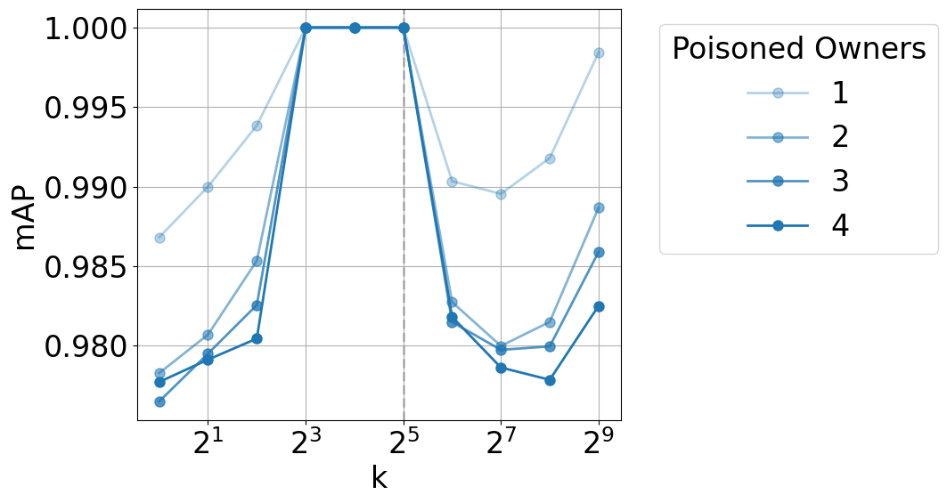
(a) BadNets mAP vs $k$

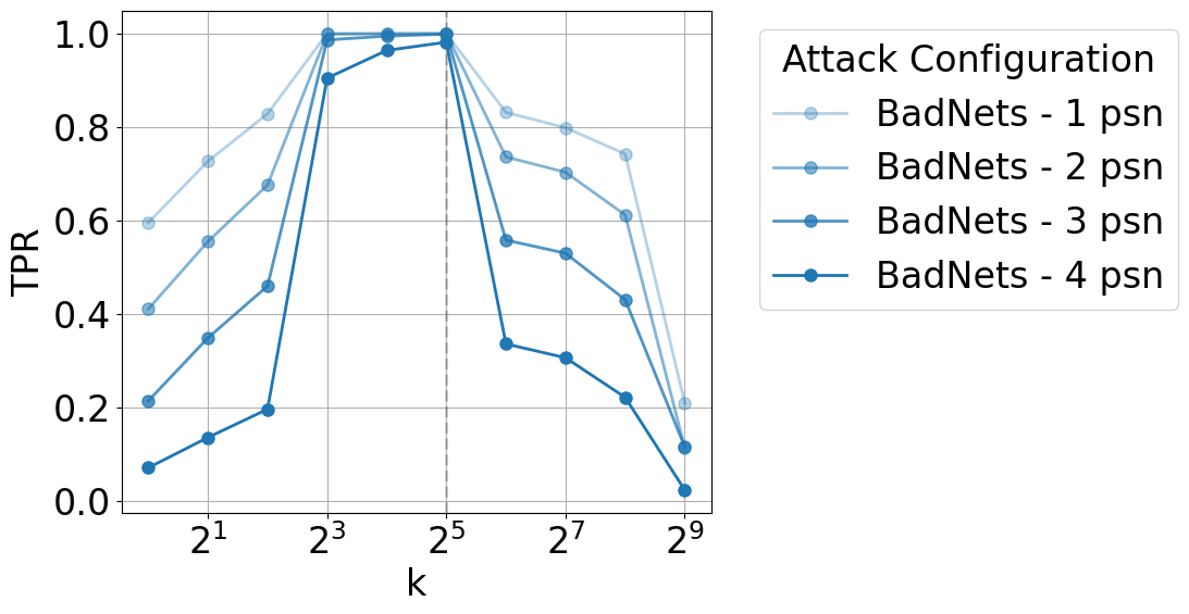
(b) BadNets TPR vs $k$

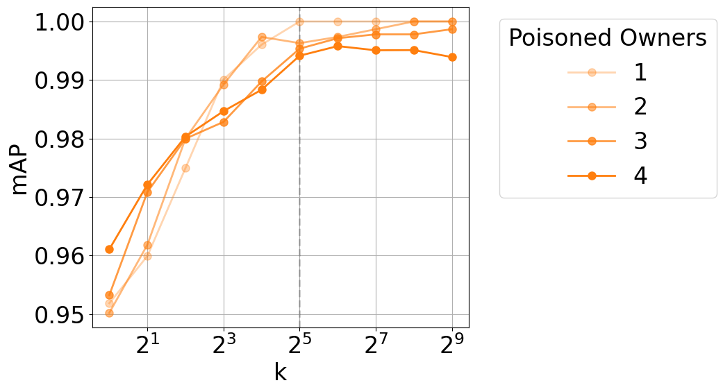
(c) Subpop mAP vs $k$

n

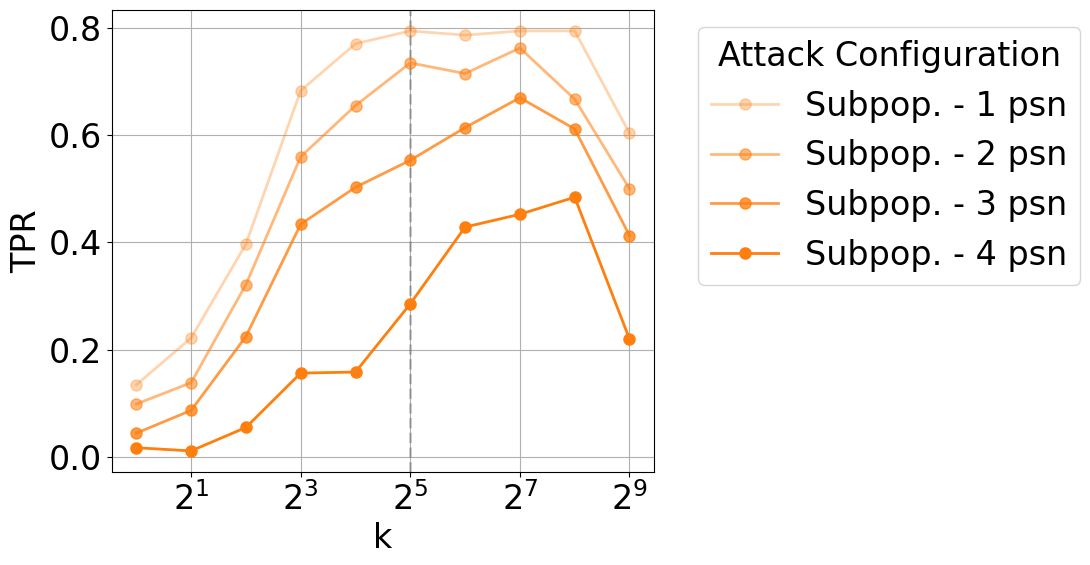
(d) Subpop TPR vs $k$

Figure 6: Hyperparameter $k$ ablation. We plot the mAP score and TPR at 0.1% FPR for various values of $k$ for BadNets and Subpopulation attacks against CIFAR-10.

20 Users Ablation. We evaluate the dependence of UTrace on the total number of users by simulating a scenario with 20 total users. We consider scenarios with 2, 4, 6, and 8 poisoned users. Results are given in Tables 7 and 8. We notice slight degradation in ranking performance for BadNets with our method, whereas unlearning maintains perfect rankings. On the other hand, using thresholds determined from FPR analysis produces relatively large FPR for unlearning, qualitatively similar to findings with 10 users. For Subpopulation attacks, the degradation under unlearning is more severe than with 10 users: a mAP of 0.903 with 4 poisoned owners and 20 users compared with 0.976 with 10 users. Our method, on the other hand, actually improves in performance with 20 users, maintaining $\geq 0.991$ mAP with up to 8 poisoned users. This trend is also reflected in the classification metrics: for Subpopulation attacks, unlearning TPR drops to 0 with 8 poisoned datasets, whereas our method achieves a TPR of 0.6022, which is better than with only 10 total users.

Table 7: Ranking metrics (mAP and mRR) for attacks against CIFAR-10 / ResNet18 with 20 users. Highest score is bold if the two methods are not identical.

Attack	Mal. Users	Unlearning		Ours
		mAP	mRR	mAP	mRR
BadNets	2	1.0000	1.0000	0.9584	0.9622
	4	1.0000	1.0000	0.9617	0.9674
	6	1.0000	1.0000	0.9644	0.9700
	8	1.0000	1.0000	0.9696	0.9785
Subpop	2	0.9844	0.9903	0.9937	0.9947
	4	0.9511	0.9838	0.9989	1.0000
	6	0.8873	0.9696	0.9943	1.0000
	8	0.9035	0.9887	0.9919	1.0000

Table 8: Classification metrics for attacks against CIFAR-10 / ResNet18 with 20 users at 0.1% FPR.

Attack	Mal. Users	Unlearning		Ours
		TPR	FPR	TPR	FPR
BadNets	2	1.0000	0.0242	0.8922	0.0012
	4	1.0000	0.0204	0.8352	0.0000
	6	1.0000	0.0144	0.6997	0.0000
	8	1.0000	0.0031	0.4322	0.0000
Subpop	2	0.4029	0.0000	0.9563	0.0040
	4	0.0825	0.0000	0.8968	0.0005
	6	0.0081	0.0000	0.7923	0.0000
	8	0.0000	0.0000	0.6022	0.0000

D.2 Fashion MNIST

We report the scores for the Fashion-MNIST / ConvNet training scenario in Table 9. In this setting, unlearning outperforms the gradient-based score, with perfect orderings across all attacks. Our method still achieves $\geq 0.943$ mAP and $\geq 0.943$ mRR.

We report results for Fashion-MNIST in Table 10. Similarly to Table 9, we observe a drop in detection rate on BadNets, achieving 72.5% TPR with 4 poisoned datasets. Unlearning achieves a FPR of over 0.8% on BadNets with 1 poisoned dataset, higher than the desired 0.1% for which the threshold was tuned, qualitatively matching the observation on CIFAR-10 in Section 5.2 that tuning thresholds for unlearning’s loss-based score can be difficult.

Table 9: Ranking metrics (mAP and mRR) scores for standard attacks against Fashion / ConvNet. Highest score is bold if the two methods are not identical.

Attack	Mal. Users	Unlearning		Ours
		mAP	mRR	mAP	mRR
BadNets	1	1.0000	1.0000	0.9425	0.9425
	2	1.0000	1.0000	0.9465	0.9449
	3	1.0000	1.0000	0.9485	0.9447
	4	1.0000	1.0000	0.9518	0.9452
LabelFlip	1	0.9972	0.9972	1.0000	1.0000
	2	0.9832	1.0000	1.0000	1.0000
	3	0.9462	0.9819	1.0000	1.0000
	4	0.9131	0.9824	1.0000	1.0000
Subpop	1	1.0000	1.0000	0.8758	0.8758
	2	0.9924	1.0000	0.9662	0.9669
	3	0.9391	0.9782	0.9681	0.9672
	4	0.9252	0.9690	0.9710	0.9696

Table 10: Classification metrics for standard attacks against Fashion / ConvNet at 0.1% FPR.

Attack	Mal. Users	Unlearning		Ours
		TPR	FPR	TPR	FPR
BadNets	1	1.0000	0.0087	0.9062	0.0016
	2	0.9984	0.0047	0.8914	0.0006
	3	0.9974	0.0040	0.8500	0.0002
	4	0.9965	0.0008	0.7516	0.0000
LabelFlip	1	0.5833	0.0000	0.9222	0.0006
	2	0.0889	0.0014	0.8667	0.0014
	3	0.0296	0.0000	0.7148	0.0000
	4	0.0069	0.0000	0.4472	0.0000
Subpop	1	0.8621	0.0000	0.7034	0.0008
	2	0.3103	0.0000	0.6621	0.0000
	3	0.0644	0.0000	0.4598	0.0000
	4	0.0069	0.0000	0.2741	0.0000

Table 11: Ranking metrics (mAP and mRR) scores for unlearning-aware attacks against Fashion / ConvNet. Highest score is bold if the two methods are not identical.

Attack	Mal. Users	Unlearning		Ours
		mAP	mRR	mAP	mRR
Noisy BadNets	1	0.9947	0.9947	1.0000	1.0000
	2	0.9614	0.9802	1.0000	1.0000
	3	0.9107	0.9820	1.0000	1.0000
	4	0.8512	0.9246	1.0000	1.0000
$\sigma$-BadNets	1	0.9987	0.9987	1.0000	1.0000
	2	0.9975	0.9986	1.0000	1.0000
	3	0.9898	0.9923	1.0000	1.0000
	4	0.9872	0.9908	0.9998	1.0000
Noisy $\sigma$-BadNets	1	0.9904	0.9904	1.0000	1.0000
	2	0.9660	0.9776	1.0000	1.0000
	3	0.8966	0.9381	1.0000	1.0000
	4	0.8690	0.9515	1.0000	1.0000

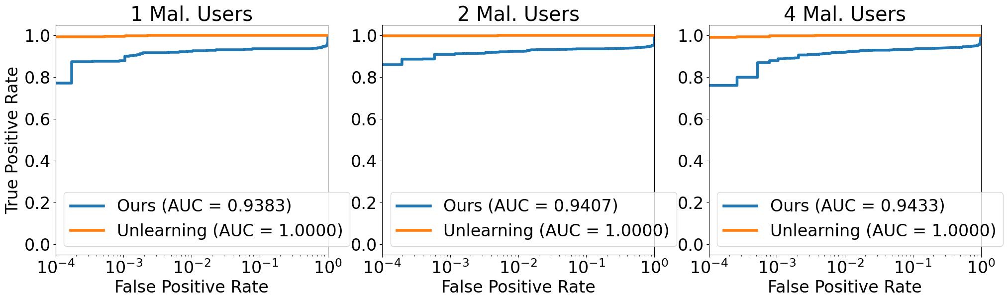
(a) BadNets

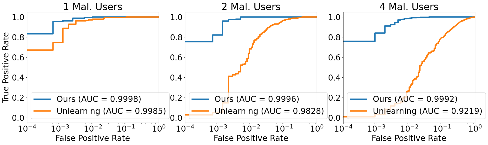
(b) Label Flip

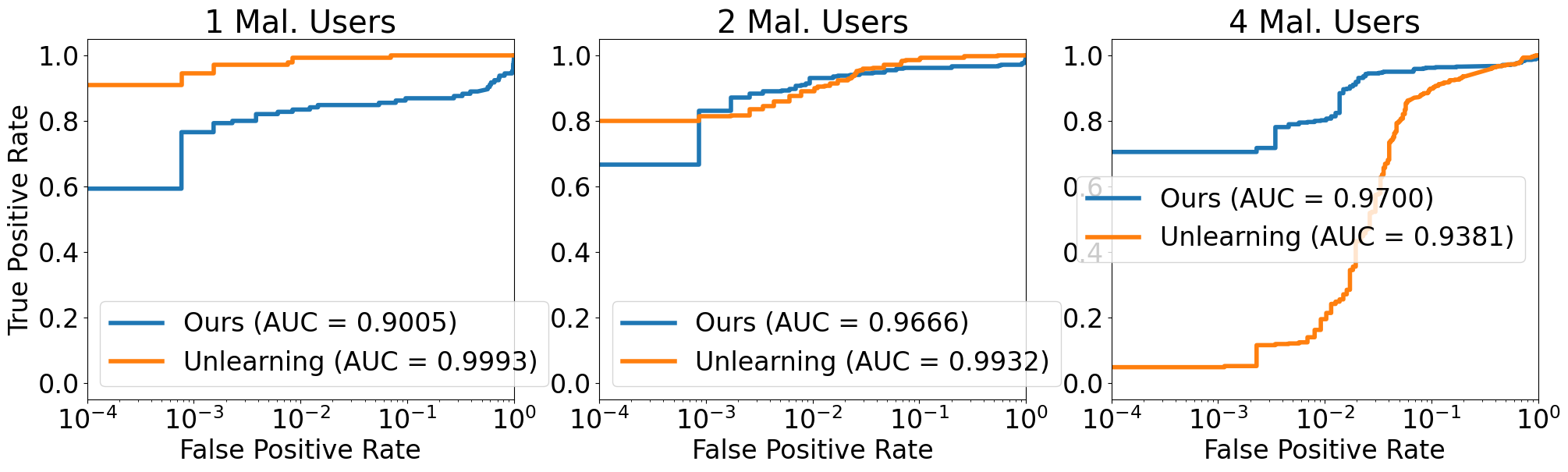
(c) Subpopulation

Figure 7: Malicious user identification ROC curves for standard attacks against Fashion / ConvNet.

(a) Noisy BadNets

(b) $\sigma$-BadNets

(c) Noisy $\sigma$-BadNets

Figure 8: Malicious user identification ROC curves for unlearning-aware attacks against Fashion / ConvNet.

Table 12: Classification metrics for unlearning-aware attacks against Fashion / ConvNet at 0.1% FPR.

Attack	Mal. Users	Unlearning		Ours
		TPR	FPR	TPR	FPR
Noisy BadNets	1	0.0734	0.0000	1.0000	0.0010
	2	0.0086	0.0000	0.9984	0.0002
	3	0.0010	0.0000	0.9984	0.0000
	4	0.0000	0.0000	0.9957	0.0000
$\sigma$-BadNets	1	0.9500	0.0002	1.0000	0.0010
	2	0.7125	0.0000	1.0000	0.0002
	3	0.3938	0.0000	0.9917	0.0000
	4	0.1484	0.0000	0.9715	0.0000
Noisy $\sigma$-BadNets	1	0.1859	0.0000	1.0000	0.0009
	2	0.0148	0.0000	0.9984	0.0000
	3	0.0010	0.0000	0.9984	0.0000
	4	0.0008	0.0003	0.9961	0.0000

D.3 Text and Malware Data Modalities

We evaluate our method on learning tasks from text and malware domains. For text, we use the SST-2 dataset [89] and fine-tune on a $\text{RoBERTa}_{\textsc{base}}$ model [65]. For malware, we use the Ember dataset [7] and train with the EmberNN model architecture [86].

Attack Setup. We perform backdoor poisoning attacks against RoBERTa/SST-2 using four backdoor variants used by Pei et al. [76] implemented in the OpenBackdoor textual backdoor toolkit [26]. Each variant implements the backdoor trigger in a different way. First, a straightforward “BadNets” extension injects a pair of arbitrary characters at a random position in the sample. For our experiments, we backdoor each poison sample with a random selection from the set $\{\text{``fe''},\text{``hr''},\text{``qp''},\text{``ge''}\}$. Second, we use a “style” backdoor that works by applying style transfer to clean examples [79]. We use the default “Bible” style for our attacks. Third, we consider a “syntax” backdoor in which the trigger is encoded in the syntactic structure of the sentence. For our experiments, we use the syntax S(SBAR)(,)(NP)(VP)(.) as the trigger. Finally, we consider a “sentence” backdoor which used the fixed sentence “I watch this 3D movie” as the trigger. The sentence backdoor is similar to the BadNets backdoor but requires a longer English phrase to appear in the sample.

For Ember / EmberNN, we consider two different backdoor attacks. First, we implement a dirty-label backdoor attack that works by choosing a random subset of features from the input space and assigning a fixed pattern to those features across all backdoored samples. We call this attack BadNets for Ember. For the remaining attack, we use the clean-label explanation-guided backdoor attack of Severi et al. [86]. For both attacks we use a poison size of 6 000 (1%).

Results. We report the ranking metrics for attacks against SST-2 / $\text{RoBERTa}_{\textsc{base}}$ in Table 16 and the classification metrics in Table 13. We report the ranking metrics for attacks against Ember / EmberNN in Table 15 and the classification metrics in Table 14. We also plot attack-conditioned ROC curves in Figures 9 and 10.

For both attacks against Ember, our method consistently achieves higher TPRs across both attack types and regardless of the number of poisoned datasets.

Despite the weaker ranking metrics under the BadNets attack with one poisoned dataset, our method still achieves better a higher TPR of 0.3281 compared to 0.0312. This discrepancy echoes the findings with the BadNets attack in Section 5.2, namely that the thresholds for the loss-based score used by approximate unlearning can depend heavily on the particular attack being considered.

One possibility is that because the explanation-guided backdoor targets features that are more relevant to the model, the terms in the gradient responsible for encoding the backdoor are more prominent than when the features are selected at random. This affects our method directly–because its effectiveness relies on alignment between poisons and attack samples–and unlearning indirectly, because the rate at which the malicious features are approximately unlearned will be slower.

Table 13: Classification metrics for attacks against SST-2 / $\text{RoBERTa}_{\textsc{base}}$ at 0.1% FPR.

Attack	Mal. Users	Unlearning		Ours
		TPR	FPR	TPR	FPR
BadNets	1	0.0312	0.0000	0.8281	0.0000
	2	0.0000	0.0000	0.7812	0.0000
	3	0.0000	0.0000	0.6719	0.0000
	4	0.0000	0.0000	0.3359	0.0000
Style	1	0.8594	0.0000	1.0000	0.0000
	2	0.5000	0.0000	1.0000	0.0000
	3	0.2552	0.0000	0.9844	0.0000
	4	0.0469	0.0000	0.8516	0.0000
Syntax	1	0.9375	0.0000	1.0000	0.0000
	2	0.6953	0.0000	0.9844	0.0000
	3	0.2135	0.0000	0.9531	0.0000
	4	0.0000	0.0000	0.5898	0.0000
Sentence	1	1.0000	0.0000	1.0000	0.0000
	2	0.2656	0.0000	1.0000	0.0000
	3	0.0000	0.0000	0.9531	0.0000
	4	0.0000	0.0000	0.8125	0.0000

Table 14: Classification metrics for attacks against Ember / EmberNN at 0.1% FPR.

Attack	Mal. Users	Unlearning		Ours
		TPR	FPR	TPR	FPR
BadNets	1	0.0312	0.0000	0.3281	0.0000
	2	0.0000	0.0000	0.1406	0.0000
	3	0.0000	0.0000	0.0521	0.0000
	4	0.0000	0.0000	0.0156	0.0000
Explanation	1	1.0000	0.0000	1.0000	0.0000
	2	0.9766	0.0000	1.0000	0.0000
	3	0.9844	0.0000	1.0000	0.0000
	4	0.0586	0.0000	0.9844	0.0000

Table 15: Ranking metrics (mAP and mRR) scores for attacks against Ember / EmberNN. Highest score is bold if the two methods are not identical.

Attack	Mal. Users	Unlearning		Ours
		mAP	mRR	mAP	mRR
BadNets	1	0.9922	0.9922	0.9672	0.9672
	2	0.9308	0.9740	0.9438	0.9688
	3	0.8516	0.9302	0.9346	0.9479
	4	0.7803	0.8560	0.9239	0.9427
Explanation	1	1.0000	1.0000	1.0000	1.0000
	2	1.0000	1.0000	1.0000	1.0000
	3	1.0000	1.0000	1.0000	1.0000
	4	1.0000	1.0000	1.0000	1.0000

Table 16: Ranking metrics (mAP and mRR) scores for attacks against SST-2 / $\text{RoBERTa}_{\textsc{base}}$. Highest score is bold if the two methods are not identical.

Attack	Mal. Users	Unlearning		Ours
		mAP	mRR	mAP	mRR
BadNets	1	1.0000	1.0000	0.9863	0.9863
	2	1.0000	1.0000	0.9803	0.9870
	3	1.0000	1.0000	0.9842	0.9896
	4	1.0000	1.0000	0.9831	0.9896
Style	1	1.0000	1.0000	1.0000	1.0000
	2	1.0000	1.0000	1.0000	1.0000
	3	1.0000	1.0000	1.0000	1.0000
	4	1.0000	1.0000	1.0000	1.0000
Syntax	1	1.0000	1.0000	1.0000	1.0000
	2	1.0000	1.0000	1.0000	1.0000
	3	1.0000	1.0000	1.0000	1.0000
	4	1.0000	1.0000	1.0000	1.0000
Sentence	1	1.0000	1.0000	1.0000	1.0000
	2	1.0000	1.0000	1.0000	1.0000
	3	1.0000	1.0000	1.0000	1.0000
	4	1.0000	1.0000	1.0000	1.0000

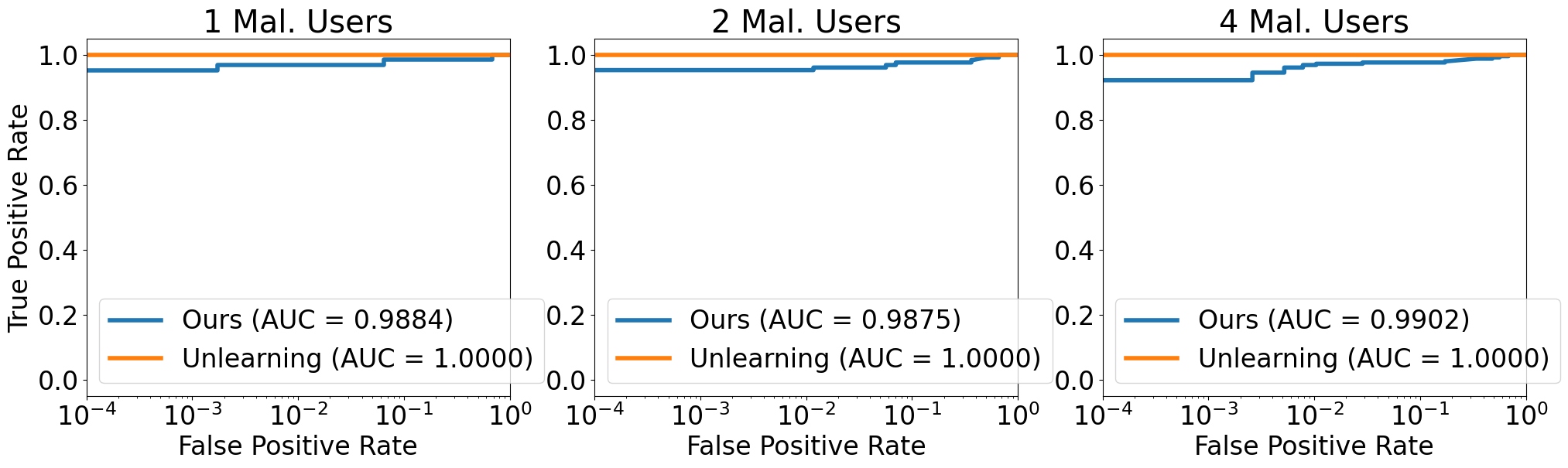
(a) BadNets

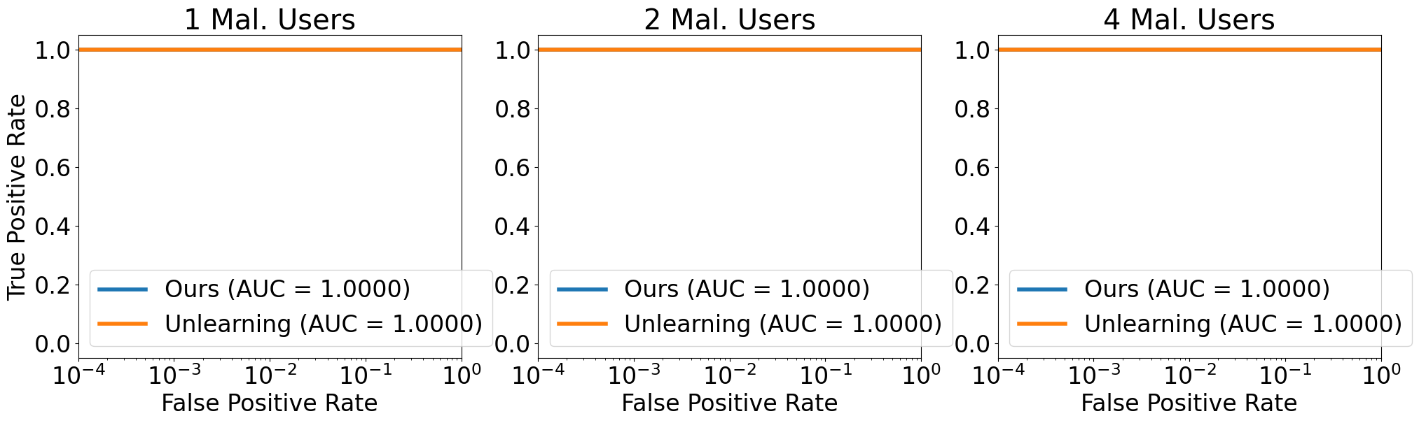
(b) Style

(c) Syntax

(d) Sentence

Figure 9: Malicious user identification ROC curves for attacks against SST-2 / $\text{RoBERTa}_{\textsc{base}}$.

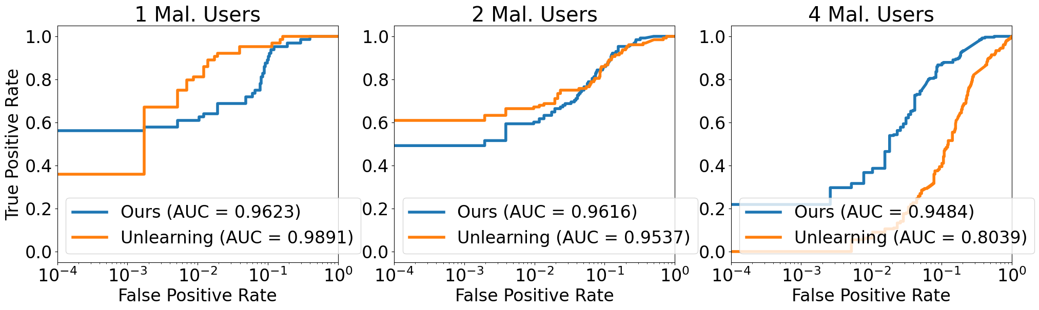
(a) BadNets

(b) Explanation

Figure 10: Malicious user identification ROC curves for attacks against Ember / EmberNN.

References

- [1] Disposal of research data - Research data security | UWE Bristol.
- [2] Regulation (EU) 2016/679 of the European Parliament and of the Council of 27 April 2016 on the protection of natural persons with regard to the processing of personal data and on the free movement of such data, and repealing Directive 95/46/EC (General Data Protection Regulation) (Text with EEA relevance), May 2016. Legislative Body: OP_DATPRO.
- [3] California Consumer Privacy Act (CCPA), October 2018.
- [4] Mark Abspoel, Daniel Escudero, and Nikolaj Volgushev. Secure training of decision trees with continuous attributes. Proceedings on Privacy Enhancing Technologies, 2021.
- [5] Hojjat Aghakhani, Dongyu Meng, Yu-Xiang Wang, Christopher Kruegel, and Giovanni Vigna. Bullseye Polytope: A Scalable Clean-Label Poisoning Attack with Improved Transferability. In 2021 IEEE European Symposium on Security and Privacy (EuroS&P), pages 159–178, September 2021.
- [6] Abdelrahaman Aly and Nigel P Smart. Benchmarking privacy preserving scientific operations. In Applied Cryptography and Network Security, pages 509–529. Springer International Publishing, 2019.
- [7] Hyrum S. Anderson and Phil Roth. EMBER: An Open Dataset for Training Static PE Malware Machine Learning Models, April 2018. arXiv:1804.04637 [cs].
- [8] Toshinori Araki, Jun Furukawa, Yehuda Lindell, Ariel Nof, and Kazuma Ohara. High-Throughput Semi-Honest Secure Three-Party Computation with an Honest Majority. In Proceedings of the 2016 ACM SIGSAC Conference on Computer and Communications Security, CCS ’16, pages 805–817, New York, NY, USA, 2016. Association for Computing Machinery. event-place: Vienna, Austria.
- [9] James Bell, Adrià Gascón, Tancrède Lepoint, Baiyu Li, Sarah Meiklejohn, Mariana Raykova, and Cathie Yun. ACORN: Input validation for secure aggregation. In 32nd USENIX Security Symposium (USENIX Security 23), pages 4805–4822, Anaheim, CA, August 2023. USENIX Association.
- [10] Michael Ben-Or, Shafi Goldwasser, and Avi Wigderson. Completeness theorems for non-cryptographic fault-tolerant distributed computation. In Proceedings of the Twentieth Annual ACM Symposium on Theory of Computing, STOC ’88, page 1–10, New York, NY, USA, 1988. Association for Computing Machinery.
- [11] Battista Biggio and Fabio Roli. Wild Patterns: Ten Years After the Rise of Adversarial Machine Learning. Pattern Recognition, 84:317–331, December 2018. arXiv:1712.03141 [cs].
- [12] California Government. California Privacy Rights Act of 2020 (CPRA), November 2020.
- [13] Xiaoyu Cao, Jinyuan Jia, Zaixi Zhang, and Neil Zhenqiang Gong. FedRecover: Recovering from Poisoning Attacks in Federated Learning using Historical Information, October 2022. arXiv:2210.10936 [cs].
- [14] Nicholas Carlini and Andreas Terzis. Poisoning and backdooring contrastive learning, 2022.
- [15] Octavian Catrina and Amitabh Saxena. Secure computation with fixed-point numbers. In Financial Cryptography and Data Security: 14th International Conference, FC 2010, Tenerife, Canary Islands, January 25-28, 2010, Revised Selected Papers 14, pages 35–50. Springer, 2010.
- [16] Nishanth Chandran, Divya Gupta, Sai Lakshmi Bhavana Obbattu, and Akash Shah. SIMC: ML Inference Secure Against Malicious Clients at Semi-Honest Cost. In 31st USENIX Security Symposium (USENIX Security 22), pages 1361–1378, Boston, MA, August 2022. USENIX Association.
- [17] Ian Chang, Katerina Sotiraki, Weikeng Chen, Murat Kantarcioglu, and Raluca Popa. HOLMES: Efficient distribution testing for secure collaborative learning. In 32nd USENIX Security Symposium (USENIX Security 23), pages 4823–4840, Anaheim, CA, August 2023. USENIX Association.
- [18] Harsh Chaudhari, Matthew Jagielski, and Alina Oprea. Safenet: The unreasonable effectiveness of ensembles in private collaborative learning. In 2023 IEEE Conference on Secure and Trustworthy Machine Learning (SaTML), pages 176–196, 2023.
- [19] Bryant Chen, Wilka Carvalho, Nathalie Baracaldo, Heiko Ludwig, Benjamin Edwards, Taesung Lee, Ian Molloy, and Biplav Srivastava. Detecting backdoor attacks on deep neural networks by activation clustering, 2018.
- [20] Ruoxin Chen, Jie Li, Chentao Wu, Bin Sheng, and Ping Li. A Framework of Randomized Selection Based Certified Defenses Against Data Poisoning Attacks, October 2020. arXiv:2009.08739 [cs, stat].
- [21] Xinyun Chen, Chang Liu, Bo Li, Kimberly Lu, and Dawn Song. Targeted backdoor attacks on deep learning systems using data poisoning, 2017.
- [22] Yudong Chen, Constantine Caramanis, and Shie Mannor. Robust High Dimensional Sparse Regression and Matching Pursuit, January 2013. arXiv:1301.2725 [cs, math, stat].
- [23] Yudong Chen, Constantine Caramanis, and Shie Mannor. Robust Sparse Regression under Adversarial Corruption. In Proceedings of the 30th International Conference on Machine Learning, pages 774–782. PMLR, May 2013. ISSN: 1938-7228.
- [24] Siyuan Cheng, Guanhong Tao, Yingqi Liu, Shengwei An, Xiangzhe Xu, Shiwei Feng, Guangyu Shen, Kaiyuan Zhang, Qiuling Xu, Shiqing Ma, and Xiangyu Zhang. BEAGLE: Forensics of Deep Learning Backdoor Attack for Better Defense. In Proceedings 2023 Network and Distributed System Security Symposium, San Diego, CA, USA, 2023. Internet Society.
- [25] Kelong Cong, Robin Geelen, Jiayi Kang, and Jeongeun Park. Revisiting oblivious top-k selection with applications to secure k -NN classification. Cryptology ePrint Archive, 2023.
- [26] Ganqu Cui, Lifan Yuan, Bingxiang He, Yangyi Chen, Zhiyuan Liu, and Maosong Sun. A Unified Evaluation of Textual Backdoor Learning: Frameworks and Benchmarks. In Proceedings of NeurIPS: Datasets and Benchmarks, 2022.
- [27] Anders Dalskov, Daniel Escudero, and Marcel Keller. Fantastic Four: Honest-Majority Four-Party Secure Computation With Malicious Security. In 30th USENIX Security Symposium (USENIX Security 21), pages 2183–2200. USENIX Association, August 2021.
- [28] I. Damgard, V. Pastro, N. P. Smart, and S. Zakarias. Multiparty computation from somewhat homomorphic encryption. Cryptology ePrint Archive, Paper 2011/535, 2011.
- [29] Ilias Diakonikolas, Gautam Kamath, Daniel Kane, Jerry Li, Jacob Steinhardt, and Alistair Stewart. Sever: A robust meta-algorithm for stochastic optimization. In Kamalika Chaudhuri and Ruslan Salakhutdinov, editors, Proceedings of the 36th International Conference on Machine Learning, volume 97 of Proceedings of Machine Learning Research, pages 1596–1606. PMLR, 09–15 Jun 2019.
- [30] European Parliament and Council of the European Union. Regulation (EU) 2016/679 of the European Parliament and of the Council, May 2016. Place: OJ L 119, 4.5.2016, p. 1–88.
- [31] Jiashi Feng, Huan Xu, Shie Mannor, and Shuicheng Yan. Robust Logistic Regression and Classification. In Advances in Neural Information Processing Systems, volume 27. Curran Associates, Inc., 2014.
- [32] Jonas Geiping, Liam Fowl, W. Ronny Huang, Wojciech Czaja, Gavin Taylor, Michael Moeller, and Tom Goldstein. Witches’ Brew: Industrial Scale Data Poisoning via Gradient Matching, May 2021. arXiv:2009.02276 [cs].
- [33] Amirata Ghorbani and James Zou. Data Shapley: Equitable Valuation of Data for Machine Learning, June 2019. arXiv:1904.02868 [cs, stat].
- [34] O. Goldreich, S. Micali, and A. Wigderson. How to play any mental game. In Proceedings of the Nineteenth Annual ACM Symposium on Theory of Computing, STOC ’87, page 218–229, New York, NY, USA, 1987. Association for Computing Machinery.
- [35] Shafi Goldwasser, Michael P. Kim, Vinod Vaikuntanathan, and Or Zamir. Planting undetectable backdoors in machine learning models, 2022.
- [36] Lukas Gosch, Mahalakshmi Sabanayagam, Debarghya Ghoshdastidar, and Stephan Günnemann. Provable Robustness of (Graph) Neural Networks Against Data Poisoning and Backdoor Attacks, July 2024. arXiv:2407.10867 [cs].
- [37] Government of Canada. Personal Information Protection and Electronic Documents Act (PIPEDA), April 2000.
- [38] Tianyu Gu, Brendan Dolan-Gavitt, and Siddharth Garg. BadNets: Identifying Vulnerabilities in the Machine Learning Model Supply Chain. IEEE Access, 7:47230–47244, March 2019. arXiv:1708.06733 [cs].
- [39] Koki Hamada, Dai Ikarashi, Koji Chida, and Katsumi Takahashi. Oblivious radix sort: An efficient sorting algorithm for practical secure multi-party computation. 2014.
- [40] Zayd Hammoudeh and Daniel Lowd. Identifying a Training-Set Attack’s Target Using Renormalized Influence Estimation. In Proceedings of the 2022 ACM SIGSAC Conference on Computer and Communications Security, pages 1367–1381, November 2022. arXiv:2201.10055 [cs].
- [41] Satoshi Hara, Atsushi Nitanda, and Takanori Maehara. Data cleansing for models trained with SGD. Curran Associates Inc., Red Hook, NY, USA, 2019.
- [42] Jonathan Hayase, Weihao Kong, Raghav Somani, and Sewoong Oh. SPECTRE: Defending against backdoor attacks using robust statistics. In Marina Meila and Tong Zhang, editors, Proceedings of the 38th International Conference on Machine Learning, volume 139 of Proceedings of Machine Learning Research, pages 4129–4139. PMLR, 18–24 Jul 2021.
- [43] Kaiming He, Xiangyu Zhang, Shaoqing Ren, and Jian Sun. Deep residual learning for image recognition. In 2016 IEEE Conference on Computer Vision and Pattern Recognition (CVPR), pages 770–778, 2016.
- [44] Alvin Heng and Harold Soh. Selective amnesia: A continual learning approach to forgetting in deep generative models, 2023.
- [45] Sanghyun Hong, Nicholas Carlini, and Alexey Kurakin. Diffusion Denoising as a Certified Defense against Clean-label Poisoning, March 2024.
- [46] Tzu-Ming Harry Hsu, Hang Qi, and Matthew Brown. Measuring the Effects of Non-Identical Data Distribution for Federated Visual Classification, September 2019. arXiv:1909.06335 [cs, stat].
- [47] Yuval Ishai, Joe Kilian, Kobbi Nissim, and Erez Petrank. Extending Oblivious Transfers Efficiently. In Dan Boneh, editor, Advances in Cryptology - CRYPTO 2003, pages 145–161, Berlin, Heidelberg, 2003. Springer.
- [48] Matthew Jagielski, Alina Oprea, Battista Biggio, Chang Liu, Cristina Nita-Rotaru, and Bo Li. Manipulating machine learning: Poisoning attacks and countermeasures for regression learning, 2021.
- [49] Matthew Jagielski, Giorgio Severi, Niklas Pousette Harger, and Alina Oprea. Subpopulation data poisoning attacks. In Proceedings of the 2021 ACM SIGSAC Conference on Computer and Communications Security, CCS ’21, page 3104–3122, New York, NY, USA, 2021. Association for Computing Machinery.
- [50] Jinyuan Jia, Xiaoyu Cao, and Neil Zhenqiang Gong. Intrinsic Certified Robustness of Bagging against Data Poisoning Attacks, December 2020. arXiv:2008.04495 [cs].
- [51] Ruoxi Jia, David Dao, Boxin Wang, Frances Ann Hubis, Nick Hynes, Nezihe Merve Gurel, Bo Li, Ce Zhang, Dawn Song, and Costas Spanos. Towards Efficient Data Valuation Based on the Shapley Value, March 2023. arXiv:1902.10275 [cs, stat].
- [52] Yuqi Jia, Minghong Fang, Hongbin Liu, Jinghuai Zhang, and Neil Zhenqiang Gong. Tracing Back the Malicious Clients in Poisoning Attacks to Federated Learning, July 2024. arXiv:2407.07221 [cs].
- [53] William B. Johnson and Joram Lindenstrauss. Extensions of Lipschitz mappings into a Hilbert space. In Conference in modern analysis and probability (New Haven, Conn., 1982), volume 26 of Contemp. Math., pages 189–206. Amer. Math. Soc., Providence, RI, 1984.
- [54] Angelos Katharopoulos and François Fleuret. Not All Samples Are Created Equal: Deep Learning with Importance Sampling, October 2019. arXiv:1803.00942 [cs].
- [55] Marcel Keller. Mp-spdz: A versatile framework for multi-party computation. In Proceedings of the 2020 ACM SIGSAC conference on computer and communications security, pages 1575–1590, 2020.
- [56] Marcel Keller and Ke Sun. Secure quantized training for deep learning. In ICML, volume 162, 2022.
- [57] Pang Wei Koh and Percy Liang. Understanding black-box predictions via influence functions. In Proceedings of the 34th International Conference on Machine Learning - Volume 70, ICML’17, page 1885–1894. JMLR.org, 2017.
- [58] Pang Wei Koh, Jacob Steinhardt, and Percy Liang. Stronger data poisoning attacks break data sanitization defenses. Mach. Learn., 111(1):1–47, jan 2022.
- [59] Alex Krizhevsky, Vinod Nair, and Geoffrey Hinton. CIFAR-10 (Canadian Institute for Advanced Research).
- [60] Alexander Levine and Soheil Feizi. Deep Partition Aggregation: Provable Defense against General Poisoning Attacks, March 2021. arXiv:2006.14768 [cs, stat] version: 2.
- [61] Chang Liu, Bo Li, Yevgeniy Vorobeychik, and Alina Oprea. Robust Linear Regression Against Training Data Poisoning. In Proceedings of the 10th ACM Workshop on Artificial Intelligence and Security, AISec ’17, pages 91–102, New York, NY, USA, November 2017. Association for Computing Machinery.
- [62] H. Liu, Y. Wu, Z. Yu, and N. Zhang. Please Tell Me More: Privacy Impact of Explainability through the Lens of Membership Inference Attack. In 2024 IEEE Symposium on Security and Privacy (SP), pages 119–119, Los Alamitos, CA, USA, May 2024. IEEE Computer Society. ISSN: 2375-1207.
- [63] Jinxin Liu and Zao Yang. Tracing Privacy Leakage of Language Models to Training Data via Adjusted Influence Functions, August 2024. arXiv:2408.10468 [cs] version: 3.
- [64] Kang Liu, Brendan Dolan-Gavitt, and Siddharth Garg. Fine-pruning: Defending against backdooring attacks on deep neural networks. In International Symposium on Research in Attacks, Intrusions, and Defenses, pages 273–294. Springer, 2018.
- [65] Yinhan Liu, Myle Ott, Naman Goyal, Jingfei Du, Mandar Joshi, Danqi Chen, Omer Levy, Mike Lewis, Luke Zettlemoyer, and Veselin Stoyanov. RoBERTa: A Robustly Optimized BERT Pretraining Approach, July 2019. arXiv:1907.11692 [cs].
- [66] Wen-Jie Lu, Yixuan Fang, Zhicong Huang, Cheng Hong, Chaochao Chen, Hunter Qu, Yajin Zhou, and Kui Ren. Faster secure multiparty computation of adaptive gradient descent. In Proceedings of the 2020 Workshop on Privacy-Preserving Machine Learning in Practice, New York, NY, USA, November 2020. ACM.
- [67] Yiwei Lu, Gautam Kamath, and Yaoliang Yu. Exploring the limits of model-targeted indiscriminate data poisoning attacks. In Proceedings of the 40th International Conference on Machine Learning, ICML’23. JMLR.org, 2023.
- [68] Yiwei Lu, Matthew Y. R. Yang, Gautam Kamath, and Yaoliang Yu. Indiscriminate data poisoning attacks on pre-trained feature extractors. In 2024 IEEE Conference on Secure and Trustworthy Machine Learning (SaTML), pages 327–343, 2024.
- [69] Hidde Lycklama, Lukas Burkhalter, Alexander Viand, Nicolas Küchler, and Anwar Hithnawi. RoFL: Robustness of secure federated learning. In IEEE Symposium on Security and Privacy (SP). IEEE, 2023.
- [70] Hidde Lycklama, Nicolas Küchler, Alexander Viand, Emanuel Opel, Lukas Burkhalter, and Anwar Hithnawi. Cryptographic Auditing for Collaborative Learning. November 2022.
- [71] Hidde Lycklama, Alexander Viand, Nicolas Küchler, Christian Knabenhans, and Anwar Hithnawi. Holding Secrets Accountable: Auditing Privacy-Preserving Machine Learning, February 2024. arXiv:2402.15780 [cs].
- [72] Naren Manoj and Avrim Blum. Excess capacity and backdoor poisoning. In M. Ranzato, A. Beygelzimer, Y. Dauphin, P.S. Liang, and J. Wortman Vaughan, editors, Advances in Neural Information Processing Systems, volume 34, pages 20373–20384. Curran Associates, Inc., 2021.
- [73] Payman Mohassel and Peter Rindal. ABY3: A mixed protocol framework for machine learning. Cryptology ePrint Archive, Paper 2018/403, 2018.
- [74] Payman Mohassel and Yupeng Zhang. Secureml: A system for scalable privacy-preserving machine learning. In 2017 IEEE Symposium on Security and Privacy (SP), pages 19–38, 2017.
- [75] Arpita Patra, Thomas Schneider, Ajith Suresh, and Hossein Yalame. ABY2.0: Improved Mixed-Protocol secure Two-Party computation. In 30th USENIX Security Symposium (USENIX Security 21), pages 2165–2182. USENIX Association, August 2021.
- [76] Hengzhi Pei, Jinyuan Jia, Wenbo Guo, Bo Li, and Dawn Song. TextGuard: Provable Defense against Backdoor Attacks on Text Classification, November 2023. arXiv:2311.11225 [cs].
- [77] Neehar Peri, Neal Gupta, W Ronny Huang, Liam Fowl, Chen Zhu, Soheil Feizi, Tom Goldstein, and John P Dickerson. Deep k-nn defense against clean-label data poisoning attacks. In European Conference on Computer Vision, pages 55–70. Springer, 2020.
- [78] Garima Pruthi, Frederick Liu, Satyen Kale, and Mukund Sundararajan. Estimating Training Data Influence by Tracing Gradient Descent. In Advances in Neural Information Processing Systems, volume 33, pages 19920–19930. Curran Associates, Inc., 2020.
- [79] Fanchao Qi, Yangyi Chen, Xurui Zhang, Mukai Li, Zhiyuan Liu, and Maosong Sun. Mind the style of text! adversarial and backdoor attacks based on text style transfer. In Marie-Francine Moens, Xuanjing Huang, Lucia Specia, and Scott Wen-tau Yih, editors, Proceedings of the 2021 Conference on Empirical Methods in Natural Language Processing, pages 4569–4580, Online and Punta Cana, Dominican Republic, November 2021. Association for Computational Linguistics.
- [80] Javier Rando and Florian Tramèr. Universal jailbreak backdoors from poisoned human feedback, 2024.
- [81] Deevashwer Rathee, Mayank Rathee, Nishant Kumar, Nishanth Chandran, Divya Gupta, Aseem Rastogi, and Rahul Sharma. Cryptflow2: Practical 2-party secure inference. In Proceedings of the 2020 ACM SIGSAC Conference on Computer and Communications Security, CCS ’20, page 325–342, New York, NY, USA, 2020. Association for Computing Machinery.
- [82] Keivan Rezaei, Kiarash Banihashem, Atoosa Chegini, and Soheil Feizi. Run-Off Election: Improved Provable Defense against Data Poisoning Attacks, May 2023. arXiv:2302.02300 [cs].
- [83] Elan Rosenfeld, Ezra Winston, Pradeep Ravikumar, and J. Zico Kolter. Certified robustness to label-flipping attacks via randomized smoothing. In Proceedings of the 37th International Conference on Machine Learning, ICML’20. JMLR.org, 2020.
- [84] Aniruddha Saha, Akshayvarun Subramanya, and Hamed Pirsiavash. Hidden-Trigger Backdoor Attacks. 34th AAAI Conference on Artificial Intelligence (AAAI) 2020, April 2020.
- [85] Avi Schwarzschild, Micah Goldblum, Arjun Gupta, John P. Dickerson, and Tom Goldstein. Just How Toxic is Data Poisoning? A Unified Benchmark for Backdoor and Data Poisoning Attacks, June 2021. arXiv:2006.12557 [cs, stat].
- [86] Giorgio Severi, Jim Meyer, Scott Coull, and Alina Oprea. Explanation-Guided backdoor poisoning attacks against malware classifiers. In 30th USENIX Security Symposium (USENIX Security 21), pages 1487–1504. USENIX Association, August 2021.
- [87] Ali Shafahi, W. Ronny Huang, Mahyar Najibi, Octavian Suciu, Christoph Studer, Tudor Dumitras, and Tom Goldstein. Poison frogs! targeted clean-label poisoning attacks on neural networks. In Proceedings of the 32nd International Conference on Neural Information Processing Systems, NIPS’18, pages 6106–6116, Red Hook, NY, USA, December 2018. Curran Associates Inc.
- [88] Shawn Shan, Arjun Nitin Bhagoji, Haitao Zheng, and Ben Y. Zhao. Poison forensics: Traceback of data poisoning attacks in neural networks. In 31st USENIX Security Symposium (USENIX Security 22), pages 3575–3592, Boston, MA, August 2022. USENIX Association.
- [89] Richard Socher, Alex Perelygin, Jean Wu, Jason Chuang, Christopher D. Manning, Andrew Ng, and Christopher Potts. Recursive Deep Models for Semantic Compositionality Over a Sentiment Treebank. In Proceedings of the 2013 Conference on Empirical Methods in Natural Language Processing, pages 1631–1642, Seattle, Washington, USA, October 2013. Association for Computational Linguistics.
- [90] Philip Sosnin, Mark N. Müller, Maximilian Baader, Calvin Tsay, and Matthew Wicker. Certified Robustness to Data Poisoning in Gradient-Based Training, June 2024. arXiv:2406.05670 [cs] version: 1.
- [91] Hossein Souri, Liam Fowl, Rama Chellappa, Micah Goldblum, and Tom Goldstein. Sleeper agent: Scalable hidden trigger backdoors for neural networks trained from scratch. In S. Koyejo, S. Mohamed, A. Agarwal, D. Belgrave, K. Cho, and A. Oh, editors, Advances in Neural Information Processing Systems, volume 35, pages 19165–19178. Curran Associates, Inc., 2022.
- [92] Jacob Steinhardt, Pang Wei W Koh, and Percy S Liang. Certified defenses for data poisoning attacks. In I. Guyon, U. Von Luxburg, S. Bengio, H. Wallach, R. Fergus, S. Vishwanathan, and R. Garnett, editors, Advances in Neural Information Processing Systems, volume 30. Curran Associates, Inc., 2017.
- [93] Fnu Suya, Xiao Zhang, Yuan Tian, and David Evans. When Can Linear Learners be Robust to Indiscriminate Poisoning Attacks?, July 2023. arXiv:2307.01073 [cs].
- [94] Brandon Tran, Jerry Li, and Aleksander Madry. Spectral signatures in backdoor attacks. In S. Bengio, H. Wallach, H. Larochelle, K. Grauman, N. Cesa-Bianchi, and R. Garnett, editors, Advances in Neural Information Processing Systems, volume 31. Curran Associates, Inc., 2018.
- [95] Sameer Wagh, Shruti Tople, Fabrice Benhamouda, Eyal Kushilevitz, Prateek Mittal, and Tal Rabin. Falcon: Honest-majority maliciously secure framework for private deep learning, 2020.
- [96] Binghui Wang, Xiaoyu Cao, Jinyuan jia, and Neil Zhenqiang Gong. On Certifying Robustness against Backdoor Attacks via Randomized Smoothing, July 2020. arXiv:2002.11750 [cs].
- [97] Bolun Wang, Yuanshun Yao, Shawn Shan, Huiying Li, Bimal Viswanath, Haitao Zheng, and Ben Y. Zhao. Neural cleanse: Identifying and mitigating backdoor attacks in neural networks. In 2019 IEEE Symposium on Security and Privacy (SP), pages 707–723, 2019.
- [98] Wenxiao Wang, Alexander Levine, and Soheil Feizi. Improved Certified Defenses against Data Poisoning with (Deterministic) Finite Aggregation, July 2022. arXiv:2202.02628 [cs, stat].
- [99] David P. Woodruff. Sketching as a Tool for Numerical Linear Algebra. Foundations and Trends® in Theoretical Computer Science, 10(1-2):1–157, 2014. arXiv:1411.4357 [cs].
- [100] Han Xiao, Kashif Rasul, and Roland Vollgraf. Fashion-MNIST: a Novel Image Dataset for Benchmarking Machine Learning Algorithms, August 2017. arXiv: cs.LG/1708.07747.
- [101] Yuhao Zhang, Aws Albarghouthi, and Loris D’Antoni. PECAN: A Deterministic Certified Defense Against Backdoor Attacks, January 2024. arXiv:2301.11824 [cs].