Photoproduction of the $\Lambda(1800)$

Abstract

We have carried out a study of the $\gamma~{}p\rightarrow pK^{+}K^{*-}(K^{*-}\rightarrow K^{-}\pi^{0})$, $\gamma~{}p\rightarrow pK^{+}K^{*-}(K^{*-}\rightarrow\bar{K}^{0}\pi^{-})$ and $\gamma~{}p\rightarrow K^{+}K^{-}p$ reactions, producing the $K^{+}\Lambda(1800)$ final state, from the perspective that the $\Lambda(1800)$ resonance is dynamically generated from the interaction of $\bar{K}^{*}N$ with its coupled vector-baryon channels, in complete analogy to the $\Lambda(1405)$ generated from the interaction of $\bar{K}N$ and its coupled pseudoscalar-baryon channels. The two reactions are complementary and their mass distributions are tied to the particular nature of this resonance in that framework. We provide much information on the shapes and strength of the invariant mass distributions of these reactions, and the energy dependence of the cross sections, that when contrasted with future experiments should shed valuable light on the nature of this resonance and its analogy to the $\Lambda(1405)$.

I introduction

Hyperons, as baryons containing one or more strange quarks, have attracted much attention in hadron physics, both experimentally Tran et al. (1998); Tovee et al. (1971); Ciborowski et al. (1982); Morelos Pineda et al. (1993); Duryea et al. (1991); Anisovich et al. (2007); Wilkinson et al. (1981); Paterson et al. (2016); de la Vaissiere et al. (1985); Goers et al. (1999); Ablikim et al. (2021); Aduszkiewicz et al. (2016); Biagi et al. (1981); Dobbs et al. (2014); Adamova et al. (2017); Chien et al. (1966); Sarantsev et al. (2019); Carmony et al. (1964); Beretvas et al. (1986); Bardadin-Otwinowska et al. (1975); Ronniger and Metsch (2011); Adamczewski-Musch et al. (2018); Crede (2023); Abazov et al. (2023); Arellano and Adriazola (2024) and theoretically Nakamura and Jido (2014); Van Cauteren et al. (2004); Jackson et al. (2015); Bernard et al. (1992); Lee (1968); Feldman et al. (1961); Sibirtsev et al. (2006); Ellis et al. (2007); Kim et al. (2013); Kaiser (2005); Ozpineci et al. (2005); Zhong and Zhao (2013); Quigg and Rosner (1976); Shi et al. (2023); Yan et al. (2023). The Lambda states have been the object of much debate, since from the very beginning, even before the $\Lambda(1405)$ was observed, the resonance had already been predicted as a $\bar{K}N$ bound state in Dalitz and Tuan (1960, 1959). The advent of the chiral unitary approach  Kaiser et al. (1995a, b); Oset and Ramos (1998); Oller et al. (2000) made this claim more transparent, and using a unitary approach in the coupled channels to $\bar{K}N$ with the input of the potentials from Chiral Lagrangians Ecker (1995); Bernard et al. (1995), two states of the $\Lambda(1405)$ were generated Oller and Meissner (2001); Jido et al. (2003) that are now reported in the PDG Navas et al. (2024). These states stem from the interaction of pseudoscalar mesons with the baryons of the octet. The extension of the idea to the interaction of vector mesons with the octet of baryons was done in Ref. Oset and Ramos (2010a), where also many dynamically generated states were obtained. In analogy to the $\Lambda(1420)$, and another $\Lambda$, the $\Lambda(1380)$, which couple mostly to $\bar{K}N$ and $\pi\Sigma$, respectively, two analogous states were generated, the $\Lambda(1800)$ coupling mostly to $\bar{K}^{*}N$ and the $\Lambda(1900)$ coupling mostly to $\rho\Sigma$. It might look surprising that now the $\bar{K}^{*}N$ state has smaller mass than the $\rho\Sigma$, compared to the $\bar{K}N$ and $\pi\Sigma$, but the large mass of the $\rho$ compared to that of the pion is responsible for it.

The analogy of the $\Lambda(1800)$ to the $\Lambda(1420)$ and the large amount of work devoted to the study of the nature of the two $\Lambda(1405)$ states Lutz and Kolomeitsev (2002); Garcia-Recio et al. (2003); Magas et al. (2005); Ikeda et al. (2012); Guo and Oller (2013); Mai and Meißner (2015); Roca and Oset (2013a, b); Cieplý et al. (2016); Cieply and Smejkal (2012); Kamiya et al. (2016); Hyodo and Weise (2008); Révai (2018); Bruns and Cieplý (2020); Miyahara and Hyodo (2018); Hyodo and Jido (2012); Meißner (2020), justifies to turn now the attention to the $\Lambda(1800)$.

Apart from data of $\bar{K}N$ going to many final states, mostly used to study the $\bar{K}N$ interaction and the related dynamically generated states, the photoproduction reaction, $\gamma p\to K\pi\Sigma$ Moriya et al. (2013a, b); Schumacher and Moriya (2013), turned out to be a rich source of information on that issue, as shown in Refs. Mai and Meißner (2015); Roca and Oset (2013a, b). From this perspective, our purpose in this work is to study theoretically the $\gamma p\to K\bar{K}N$ and $\gamma p\to K\bar{K}^{*}N$ reactions, with the aim of learning about the nature of this $\Lambda(1800)$ state. The reactions proposed can be easily implemented in present facilities, like Jefferson Lab.

II Formalism

To investigate the photoproduction of the $\Lambda(1800)$, we will employ two mechanisms.

II.1 Formalism for the photoproduction of $\gamma~{}p\rightarrow pK^{+}K^{*-}(K^{*-}\rightarrow K^{-}\pi^{0})$ and $\gamma~{}p\rightarrow pK^{+}K^{*-}(K^{*-}\rightarrow\bar{K}^{0}\pi^{-})$ Reactions

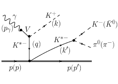
Figure 1: Mechanism of the photoproduction reaction $\gamma~{}p\rightarrow pK^{+}K^{*-}(K^{*-}\rightarrow K^{-}\pi^{0})$ and $\gamma~{}p\rightarrow pK^{+}K^{*-}(K^{*-}\rightarrow\bar{K}^{0}\pi^{-})$. The symbol $V$ stands for the $\rho^{0}$, $\omega$ and $\phi$ vector mesons.

The mechanism for the $\gamma~{}p\rightarrow pK^{+}K^{*-}(K^{*-}\rightarrow K^{-}\pi^{0})$ and $\gamma~{}p\rightarrow pK^{+}K^{*-}(K^{*-}\rightarrow\bar{K}^{0}\pi^{-})$ process is shown in Fig. 1. First, we calculate the $\gamma\rightarrow K^{+}K^{*-}$ vertex. As depicted in Fig. 1, we rely upon vector meson dominance, where the photon converts into a vector meson $V(\rho^{0},\omega,\phi)$, which subsequently interacts with $K^{+}$ and $K^{*-}$ mesons. The photon conversion into $V$ is derived from the Local Hidden Gauge Lagrangian Bando et al. (1985, 1988); Meissner (1988) as described in Nagahiro et al. (2009):

$${\cal L}_{\gamma V}=-M^{2}_{V}\frac{e}{g}A_{\mu}\langle V^{\mu}Q\rangle$$ (1)

where $A_{\mu}$ and $V^{\mu}$ represent the photon and vector meson fields, respectively, and $Q=1/3(2,-1,-1)$ is the charge matrix of the $u$, $d$, and $s$ quarks. In Eq. (1), $g$ is the universal coupling in the Local Hidden Gauge Lagrangian, given by $g=M_{V}/(2f_{\pi})$, where $M_{V}$ is an appropriate vector meson mass (we take $800$ MeV) and $f_{\pi}=93$ MeV is the pion decay constant. The constant $e$ is the charge of the electron, normalized such that $e^{2}/(4\pi)=\alpha=1/137$.

The other ingredient we need is the $V(\rho^{0},\omega,\phi)K^{+}K^{*-}$ vertex, which is described by the anomalous Lagrangian Bramon et al. (1992):

$${\cal L}_{VVP}=\frac{G^{\prime}}{\sqrt{2}}\epsilon^{\mu\nu\alpha\beta}\langle\partial_{\mu}V_{\nu}\partial_{\alpha}V_{\beta}P\rangle$$ (2)

where $V$ is the matrix of vector meson nonet SU (3) matrices:

$$V=\begin{pmatrix}\frac{1}{\sqrt{2}}\rho^{0}+\frac{1}{\sqrt{2}}\omega&\rho^{+}&K^{*+}&\\ \rho^{-}&-\frac{1}{\sqrt{2}}\rho^{0}+\frac{1}{\sqrt{2}}\omega&K^{*0}\\ K^{*-}&\bar{K}^{*0}&\phi\end{pmatrix},$$ (3)

and $P$ is the matrix of pseudoscalar fields:

$$P=\begin{pmatrix}\frac{1}{\sqrt{2}}\pi^{0}+\frac{1}{\sqrt{3}}\eta+\frac{1}{\sqrt{6}}\eta^{\prime}&\pi^{+}&K^{+}&\\ \pi^{-}&-\frac{1}{\sqrt{2}}\pi^{0}+\frac{1}{\sqrt{3}}\eta+\frac{1}{\sqrt{6}}\eta^{\prime}&K^{0}\\ K^{-}&\bar{K}^{0}&-\frac{1}{\sqrt{3}}\eta+\sqrt{\frac{2}{3}}\eta^{\prime}\end{pmatrix},$$ (4)

with the $\eta$-$\eta^{\prime}$ mixing of Ref. Bramon et al. (1992), with the symbol $\langle~{}\rangle$ representing the trace in $SU(3)$ space. In Eq. (2), $G^{\prime}$ is the coupling constant of the $VVP$ Lagrangian which is given by:

$$G^{\prime}=\dfrac{3g^{\prime 2}}{4\pi^{2}f}~{}~{};~{}~{}~{}g^{\prime}=-\dfrac{G_{V}M_{V}}{\sqrt{2}f^{2}}.$$ (5)

and $G_{V}$ is the coupling of $\rho$ to two pions, which, as in Oset et al. (2003, 2008) we take as $G_{V}=69$ MeV $(G’=0.0154~{}\mathrm{MeV}^{-1}$) and $G_{V}=55$ MeV ($G’=0.0098~{}\mathrm{MeV}^{-1}$). We take the average $G^{\prime}=0.012$ $\mathrm{MeV}^{-1}$.

Using Eqs. (2, 3, 4), the $VK^{*-}K^{+}$ vertex can be evaluated as follows:

$$-i~{}t=i~{}\frac{G^{\prime}}{\sqrt{2}}\frac{1}{3}\frac{e}{g}\epsilon^{\mu\nu\alpha\beta}(-i~{}p_{\gamma})_{\mu}\epsilon_{\nu}(\gamma)(i~{}q_{\alpha})\epsilon_{\beta}(K^{*-})$$ (6)

We choose to evaluate this amplitude in the $K^{*-}p$ rest frame where the amplitude is in $S$-wave, which leads us to take $\epsilon^{\mu\nu\alpha\beta}q^{\alpha}\to\epsilon^{\mu\nu 0\beta}q^{0}$. For the photon, we work in the Coulomb Gauge, $\epsilon^{0}(0)=0$, and the photons have only the transverse polarizations. With these considerations, we obtain the following result:

$$-i~{}t =i~{}\frac{G^{\prime}}{\sqrt{2}}\frac{1}{3}\frac{e}{g}\epsilon^{\mu\nu 0\beta}p_{\gamma,\mu}\epsilon_{\nu}(\gamma)q_{0}\epsilon_{\beta}(K^{*-})$$

$$=-i~{}\frac{G^{\prime}}{\sqrt{2}}\frac{1}{3}\frac{e}{g}\epsilon^{ijl}p_{\gamma}^{i}\epsilon^{j}(\gamma)q^{0}\epsilon^{l}(K^{*-})$$ (7)

Now we introduce the $K^{*-}$ propagator and the $K^{*-}p\rightarrow K^{*-}p$ amplitude:

$$i~{}\dfrac{1}{(q^{0})^{2}-\vec{q}^{~{}2}-m^{2}_{K^{*}}}~{}(-i)~{}t_{K^{*-}p\rightarrow K^{*-}p}(M_{\mathrm{inv}})~{}~{}\epsilon^{m}(K^{*-}(\mathrm{ingoing}))~{}\epsilon^{m}(K^{*-}(\mathrm{outgoing}))$$ (8)

where the $K^{*-}p\rightarrow K^{*-}p$ amplitude is calculated in Ref. Oset and Ramos (2010b) using the Local Hidden Gauge formalism with a coupled-channels unitary approach in the isospin basis. Additionally, Ref. Garzon and Oset (2012) includes the box diagram involving the exchange of pseudoscalar mesons. However, we will use a Breit Wigner amplitude to account empirically for the $\Lambda(1800)$ experimental width, which is larger than predicted by the theory:

$$t_{K^{*-}p\rightarrow K^{*-}p}=\dfrac{g_{K^{*-}p}^{2}}{M_{\mathrm{inv}}(K^{*-}p)-M_{\Lambda(1800)}+i\frac{\Gamma_{\Lambda}(1800)}{2}}.$$ (9)

with $M_{\Lambda(1800)}=1809$ MeV and $\Gamma_{\Lambda}(1800)=200$ MeV. Here, $g_{K^{*-}p}$ is the coupling constant, which was calculated in Ref. Garzon and Oset (2012) in the isospin basis. Hence the coupling constant to $K^{*-}p$ is $|g_{K^{*-}p}|=\dfrac{1}{\sqrt{2}}|g^{I=0}_{\bar{K}^{*}N}|=2.83$. (Our isospin multiplets are ($K^{*+}$, $K^{*0}$), ( $\bar{K}^{*0}$ ,$-K^{*-}$)).

For the amplitude corresponding to the mechanism in Fig. 1, we average $|t_{\gamma p\rightarrow K^{+}K^{*-}p}|^{2}$ over the spin of the incoming particles and sum over the spin of the outgoing particles. However, since there is no spin dependence on the protons in the $t_{K^{*-}p\rightarrow K^{*-}p}$ amplitude, summing and averaging over the proton polarizations gives us a factor of $1$. Then, we get:

$$\overline{\sum}\sum|t_{\gamma p\rightarrow K^{+}K^{*-}p}|^{2}=\left(\dfrac{G^{\prime}}{3\sqrt{2}}\frac{e}{g}q^{0}\right)^{2}\left|\dfrac{1}{(q^{0})^{2}-\vec{q}^{~{}2}-m^{2}_{K^{*}}}\right|^{2}\left|t_{K^{*-}p\rightarrow K^{*-}p}\right|^{2}\vec{p}^{~{}2}_{\gamma}$$ (10)

where the magnitudes $q^{0}$ and $p_{\gamma}$ are evaluated in the $K^{*-}p$ rest frame. However, since the $K^{*-}$ propagator is invariant, it is more convenient to evaluate it in the $\gamma p$ rest frame as:

$$\dfrac{1}{(q^{0})^{2}-\vec{q}^{~{}2}-m^{2}_{K^{*}}}=\dfrac{1}{-2p_{\gamma/\mathrm{c.m}}[\omega(k)-kcos\theta]+m^{2}_{K}-m^{2}_{K^{*}}-im_{K^{*}}\Gamma_{K^{*}}}.$$ (11)

Here, $p_{\gamma/\mathrm{c.m}}=(s-m^{2}_{p})/2\sqrt{s}$ represents the photon momentum in the $\gamma p$ rest frame, and $K$ and $\theta$ are the kaon momentum and the angle between the kaon and the proton in that frame. We multiply the $K^{*-}$ propagator by a form factor, $F(q)=\Lambda^{2}/(\Lambda^{2}+\vec{q}^{~{}2})$, where $\Lambda=1000$ MeV.

The magnitudes $q^{0}$ and $p_{\gamma}$ in Eq (10), have to be then evaluated in the $K^{*-}p$ rest frame and they are given by

$$p_{\gamma}=\dfrac{p_{\gamma/\mathrm{c.m}}}{M_{\mathrm{inv}}}\left\{E_{p}(p_{\gamma/\mathrm{c.m}})+p_{\gamma/\mathrm{c.m}}-\omega(k)+k~{}cos\theta\right\}$$ (12)

$$q^{0}=\dfrac{1}{M_{\mathrm{inv}}}\left\{[p_{\gamma/\mathrm{c.m}}-\omega(k)][\sqrt{s}-\omega(k)]+p_{\gamma/\mathrm{c.m}}kcos\theta-k^{2}\right\}.$$ (13)

Finally, to evaluate the phase space and the cross section, we take the photon in the $z$ direction. Using the Mandl and Shaw normalization Mandl and Shaw (1985), the cross section is:

$$\sigma =\dfrac{4m^{2}_{p}}{2(s-m^{2}_{p})}\int\dfrac{d^{3}k}{(2\pi)^{3}}\dfrac{1}{2\omega(k)}\,\int\dfrac{d^{3}k^{\prime}}{(2\pi)^{3}}\dfrac{1}{2\omega(k^{\prime})}\,\int\dfrac{d^{3}p^{\prime}}{(2\pi)^{3}}\dfrac{1}{2E(p^{\prime})}\,$$

$$\times\overline{\sum}\sum|t_{\gamma p\rightarrow K^{+}K^{*-}p}|^{2}~{}(2\pi)^{4}~{}\delta^{4}(p_{\gamma}+p-k-k^{\prime}-p^{\prime})$$ (14)

Taking into account that $d^{3}q/2\omega(q)$ is a Lorentz invariant, we evaluate the $k^{\prime}$ and $p^{\prime}$ integrals in the frame where $\vec{p}_{\gamma}+\vec{p}-\vec{k}=0$. Using the same argument, the $k$ integral is then evaluated in the $\gamma p$ rest frame. Then the cross section is:

$$\sigma=\dfrac{2m^{2}_{p}}{(s-m^{2}_{p})}\dfrac{1}{32\pi^{3}}\frac{1}{\sqrt{s}}\int_{M_{\mathrm{inv/min}}}^{M_{\mathrm{inv/max}}}dM_{\mathrm{inv}}(K^{*-}p)\,\int_{-1}^{+1}d(cos\theta)\,\overline{\sum}\sum|t_{\gamma p\rightarrow K^{+}K^{*-}p}|^{2}k~{}k^{\prime}$$ (15)

where $M_{\mathrm{inv}}(K^{*-}p)$ is the invariant mass of the $K^{*-}p$ system and $s$ the ordinary Mandelstam variable for the center-of-mass (c.m.) energy of the $\gamma p$ initial system. The angle $\theta$ is the angle between the $K^{+}$ and the photon in the $\gamma p$ rest frame. The momenta $k$ and $k^{\prime}$ are obtained as:

$$\omega(k)=\dfrac{s+m^{2}_{K}-M^{2}_{\mathrm{inv}}}{2\sqrt{s}};~{}~{}~{}~{}~{}~{}~{}~{}~{}~{}k=\sqrt{\omega(k)^{2}-m^{2}_{K}},$$

$$k^{\prime}=\dfrac{\lambda^{1/2}(M^{2}_{\mathrm{inv}},m^{2}_{K^{*}},m^{2}_{p})}{2M_{\mathrm{inv}}},$$ (16)

where $M_{\mathrm{inv}}$ stands for $M_{\mathrm{inv}}(K^{*-}p)$ and $\lambda$ is the Källén function.

Finally, since the $K^{*-}$ is an unstable particle, with a width, or equivalently, it has a mass distribution, we must then consider this mass distribution given by the spectral function. The decay channels are $\pi K$ and we choose the $\pi^{-}\bar{K}^{0}$ channel, for its observation. Then we have

$$\dfrac{d\sigma}{d\tilde{M}_{K^{*}}}=-\frac{1}{\pi}2\tilde{M}_{K^{*}}\texttt{Im}\dfrac{1}{\tilde{M}^{2}_{K^{*}}-M_{K^{*}}^{2}+i\tilde{M}_{K^{*}}\Gamma(\tilde{M}_{K^{*}})}\sigma(\tilde{M}_{K^{*}})$$ (17)

where $\tilde{M}_{K^{*}}$ is equal to $M_{\mathrm{inv}}(\pi^{-}\bar{K}^{0})$ and $\Gamma(\tilde{M}_{K^{*}})$ is given by;

$$\Gamma(\tilde{M}_{K^{*}})=\dfrac{M_{K^{*}}^{2}}{\tilde{M}^{2}_{K^{*}}}\left(\dfrac{p_{\pi}}{p_{\pi,\mathrm{on}}}\right)^{3}\Gamma_{\mathrm{on}}$$ (18)

with $\Gamma_{\mathrm{on}}=51.4$ MeV, the $K^{*-}$ width, and

$$p_{\pi}=\dfrac{\lambda^{1/2}(\tilde{M}^{2}_{K^{*}},m^{2}_{\pi},m^{2}_{K})}{2\tilde{M}_{K^{*}}},~{}~{}~{}~{}~{}~{}~{}~{}~{}p_{\pi,\mathrm{on}}=\dfrac{\lambda^{1/2}(M^{2}_{K^{*}},m^{2}_{\pi},m^{2}_{K})}{2M_{K^{*}}}.$$ (19)

Since the $K^{*}$ has an isospin of $\frac{1}{2}$, searching for the $K^{*-}$ in the $\pi^{-}\bar{K}^{0}$ channel, we have

$$|\pi K;\frac{1}{2},-\frac{1}{2}\rangle=-\frac{1}{\sqrt{3}}|\pi^{0}K^{-}\rangle-\sqrt{\frac{2}{3}}|\pi^{-}\bar{K}^{0}\rangle$$ (20)

then we must multiply the Eq. (17) by $2/3$ if we select the $\pi^{-}\bar{K}^{0}$ decay mode.

Thus, finally, we get, for $\pi^{-}\bar{K}^{0}$ final decay product of the $K^{*-}$,

$$\dfrac{d\sigma}{dM_{\mathrm{inv}}(\pi^{-}\bar{K}^{0})~{}~{}dM_{\mathrm{inv}}(K^{*-}p)} =-\frac{4}{3\pi}M_{\mathrm{inv}}(\pi^{-}\bar{K}^{0})\texttt{Im}\dfrac{1}{M^{~{}2}_{\mathrm{inv}}(\pi^{-}\bar{K}^{0})-M_{K^{*}}^{2}+iM_{\mathrm{inv}}(\pi^{-}\bar{K}^{0})\Gamma(M_{\mathrm{inv}}(\pi^{-}\bar{K}^{0}))}$$

$$\dfrac{2m^{2}_{p}}{(s-m^{2}_{p})}\dfrac{1}{32\pi^{3}}\frac{1}{\sqrt{s}}\int_{-1}^{+1}d(cos\theta)\,\overline{\sum}\sum|t_{\gamma p\rightarrow K^{+}K^{*-}p}|^{2}k~{}k^{\prime}$$ (21)

where $M_{\mathrm{inv}}(K^{*-}p)$ is equal to $M_{\mathrm{inv}}(\pi^{-}\bar{K}^{0}p)$ and $k^{\prime}$ of Eq. (16) is now given by

$$k^{\prime}=\dfrac{\lambda^{1/2}(M^{2}_{\mathrm{inv}}(K^{*-}p),M^{2}_{\mathrm{inv}}(\pi^{-}\bar{K}^{0}),m^{2}_{p})}{2M_{\mathrm{inv}}(K^{*-}p)}.$$ (22)

We have conducted the calculations for the $\pi^{-}\bar{K}^{0}$ decay mode of the ${K}^{*-}$. Should we have taken instead the $\pi^{0}K^{-}$ decay mode, the same results can be used substituting $2/3$ by $1/3$ according to Eq. (20).

II.2 Formalism for $\gamma~{}p\rightarrow K^{+}K^{-}p$ Reaction and Contact Term

In Fig. 2, we present the Feynman diagram for the $\gamma~{}p\rightarrow K^{+}K^{-}p$ reaction. To calculate this process, we need to evaluate two additional vertices that differ from those in Fig. 1: the upper vertex, $K^{*-}\rightarrow K^{-}\pi^{0}$, and the lower vertex, $\pi^{0}pp$

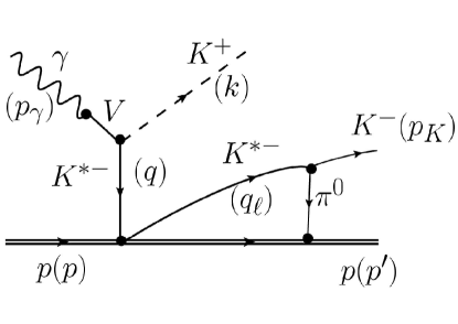
Figure 2: Feynman Diagram of $\gamma~{}p\rightarrow K^{+}K^{-}p$. The symbol $V$ stands for the $\rho^{0}$, $\omega$ and $\phi$ vector mesons.

The Lagrangian for the upper vertex (VPP vertex) is given by

$${\cal L}_{VPP} =-ig\langle[P,\partial_{\mu}P]V^{\mu}\rangle$$ (23)

$$g =\dfrac{M_{V}}{2f}~{}(M_{V}\simeq 800~{}\mathrm{MeV},f=93~{}\mathrm{MeV}).$$

Using the above Lagrangian, one obtains the following expression for the upper vertex:

$$-it=i{\cal L}=-ig\frac{1}{\sqrt{2}}\vec{\epsilon}~{}(K^{*})(\vec{p}_{K}-\vec{p}_{\pi}).$$

where $\vec{p}_{K}$ represents the momentum of the outgoing $K^{-}$ meson, and $\vec{p}_{\pi}$ the momentum of the intermediate pion. For the lower vertex, we apply the results from Ref. (Garzon and Oset, 2012):

$$-i{t}=\dfrac{D+F}{2f}\vec{\sigma}\cdot\vec{p}_{\pi}$$ (24)

with $D=0.75$ and $F=0.51$.

The amplitude corresponding to the Feynman Diagram in Fig. 2 is given by

$$-i~{}t_{L} =i~{}e\frac{G^{\prime}}{\sqrt{2}}\frac{1}{3\sqrt{2}}\dfrac{D+F}{2f}\epsilon^{ijm}p^{i}_{\gamma}\epsilon^{j}_{\gamma}q^{0}\dfrac{1}{(q^{0})^{2}-\vec{q}^{~{}2}-m^{2}_{K^{*}}+i~{}\epsilon}t_{K^{*-}p,K^{*-}p}(M_{\mathrm{inv}})$$

$$\int\frac{d^{4}q_{\ell}}{(2\pi)^{4}}\dfrac{1}{q_{\ell}^{2}-m^{2}_{K^{*}}+i~{}\epsilon}\dfrac{M_{p}}{E(\vec{P}-\vec{q_{\ell}})}\dfrac{1}{P^{0}-q^{0}_{\ell}-E(\vec{P}-\vec{q_{\ell}})+i~{}\epsilon}$$

$$\dfrac{1}{p_{\pi}^{2}-m^{2}_{\pi}+i~{}\epsilon}\vec{\sigma}\cdot\vec{p}_{\pi}~{}(\vec{p}_{K}-\vec{p}_{\pi})^{m}$$ (25)

After performing the $q_{l}^{0}$ integration analytically, we obtain

$$-i~{}t_{L} =e\frac{G^{\prime}}{\sqrt{2}}\frac{1}{3\sqrt{2}}\dfrac{D+F}{2f}q^{0}\dfrac{1}{(q^{0})^{2}-\vec{q}^{~{}2}-m^{2}_{K^{*}}+i~{}\epsilon}t_{K^{*-}p,K^{*-}p}(M_{\mathrm{inv}})$$

$$\epsilon^{ijm}p^{i}_{\gamma}\epsilon^{j}_{\gamma}\sigma^{r}\left[A~{}p^{2}_{K}~{}\delta_{rm}+B~{}p_{K,r}~{}p_{K,m}\right]$$ (26)

where

$$A =\frac{1}{{2}}\int\frac{d^{3}\vec{q}_{\ell}}{(2\pi)^{3}}\frac{1}{2\omega_{\pi}(\vec{q}_{\ell}-\vec{p}_{K})}\frac{1}{2\omega_{K^{*}}(\vec{q}_{\ell})}\dfrac{M_{p}}{E(\vec{q_{\ell}})}\dfrac{1}{M_{\mathrm{inv}}-E(\vec{q}_{\ell})-\omega_{K^{*}}(\vec{q}_{\ell})+i\dfrac{\Gamma_{K^{*}}}{2}}\theta(q_{\rm max}-|\vec{q}_{\ell}|)$$

$$\left\{\dfrac{1}{M_{\mathrm{inv}}-E(\vec{q}_{\ell})-p_{K}^{0}-\omega_{\pi}(\vec{q}_{\ell}-\vec{p}_{K})+i\epsilon}+\dfrac{1}{p_{K}^{0}-\omega_{K^{*}}(\vec{q}_{\ell})-\omega_{\pi}(\vec{q}_{\ell}-\vec{p}_{K})+i\dfrac{\Gamma_{K^{*}}}{2}}\right\}$$

$$\left\{\dfrac{1}{\vec{p}^{~{}2}_{K}}~{}(\vec{q}_{\ell}-\vec{p}_{K})\cdot(2\vec{p}_{K}-\vec{q}_{\ell})-\dfrac{1}{\vec{p}^{~{}4}_{K}}\left[(\vec{q}_{\ell}-\vec{p}_{K})\cdot\vec{p}_{K}\right]\left[(2\vec{p}_{K}-\vec{q}_{\ell})\cdot\vec{p}_{K}\right]\right\}$$ (27)

and

$$B =-\frac{1}{{2}}\int\frac{d^{3}\vec{q}_{\ell}}{(2\pi)^{3}}\frac{1}{2\omega_{\pi}(\vec{q}_{\ell}-\vec{p}_{K})}\frac{1}{2\omega_{K^{*}}(\vec{q}_{\ell})}\dfrac{M_{p}}{E(\vec{q_{\ell}})}\dfrac{1}{M_{\mathrm{inv}}-E(\vec{q}_{\ell})-\omega_{K^{*}}(\vec{q}_{\ell})+i\dfrac{\Gamma_{K^{*}}}{2}}\theta(q_{\rm max}-|\vec{q}_{\ell}|)$$

$$\left\{\dfrac{1}{M_{\mathrm{inv}}-E(\vec{q}_{\ell})-p_{K}^{0}-\omega_{\pi}(\vec{q}_{\ell}-\vec{p}_{K})+i\epsilon}+\dfrac{1}{p_{K}^{0}-\omega_{K^{*}}(\vec{q}_{\ell})-\omega_{\pi}(\vec{q}_{\ell}-\vec{p}_{K})+i\dfrac{\Gamma_{K^{*}}}{2}}\right\}$$

$$\left\{\dfrac{1}{\vec{p}^{~{}2}_{K}}~{}(\vec{q}_{\ell}-\vec{p}_{K})\cdot(2\vec{p}_{K}-\vec{q}_{\ell})-\dfrac{3}{\vec{p}^{~{}4}_{K}}\left[(\vec{q}_{\ell}-\vec{p}_{K})\cdot\vec{p}_{K}\right]\left[(2\vec{p}_{K}-\vec{q}_{\ell})\cdot\vec{p}_{K}\right]\right\}.$$ (28)

The factor $\theta(q_{\rm max}-|\vec{q}_{\ell}|)$ in Eqs. (27) and (28) is introduced because the $t$ matrix $t_{K^{*-}p,K^{*-}p}(\vec{q}_{\ell},M_{\mathrm{inv}})$ inside a loop factorizes as $t_{K^{*-}p,K^{*-}p}(M_{\mathrm{inv}})\theta(q_{\rm max}-|\vec{q}_{\ell}|)$, where $q_{\mathrm{max}}$ is the cut off used to regulate the $G$ function in the study of $VB\rightarrow VB$ scattering matrix ( see Ref. Gamermann et al. (2010)). Here, $p_{K}$ and $p_{K}^{0}$ are defined as follows:

$$p_{K}=\dfrac{\lambda^{1/2}(M^{2}_{\mathrm{inv}}(K^{-}p),m^{2}_{K^{-}},m^{2}_{p})}{2M_{\mathrm{inv}}(K^{-}p)},~{}~{}~{}~{}p_{K}^{0}=\dfrac{M^{2}_{\mathrm{inv}}(K^{-}p)+m^{2}_{K^{-}}-m^{2}_{p}}{2M_{\mathrm{inv}}(K^{-}p)}$$ (29)

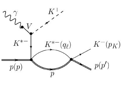
Figure 3: Feynman Diagram of the contact term.

To ensure gauge invariance in gamma $N\rightarrow KN$ when vector meson dominance is used, converting the photon into a vector meson, a contact term has to be introduced Garzon and Oset (2012) in $K^{*}N\rightarrow KN$. This contact term should be added to the amplitudes in Eq. (25). The contact term for the $K^{*}N\to KN$ amplitude is given by

$$-i\tilde{t}_{\mathrm{cont}}=-g\frac{1}{\sqrt{2}}\dfrac{D+F}{2f}\vec{\epsilon}\cdot\vec{\sigma}$$ (30)

The corresponding Feynman diagram is shown in Fig. 3, and the matrix element given by

$$-i~{}t^{(C)}_{L} =-i~{}e\frac{G^{\prime}}{\sqrt{2}}\frac{1}{3\sqrt{2}}\dfrac{D+F}{2f}\epsilon^{ijm}p^{i}_{\gamma}\epsilon^{j}_{\gamma}q^{0}\sigma^{m}\dfrac{1}{(q^{0})^{2}-\vec{q}^{~{}2}-m^{2}_{K^{*}}+i~{}\epsilon}t_{K^{*-}p,K^{*-}p}(M_{\mathrm{inv}})$$

$$\int\frac{d^{4}q_{\ell}}{(2\pi)^{4}}\dfrac{1}{q_{\ell}^{2}-m^{2}_{K^{*}}+i~{}\epsilon}\dfrac{M_{p}}{E(\vec{P}-\vec{q_{\ell}})}\dfrac{1}{P^{0}-q^{0}_{\ell}-E(\vec{P}-\vec{q_{\ell}})+i~{}\epsilon}\theta(q_{\rm max}-|\vec{q}_{\ell}|)$$ (31)

As we observe from Eq. (31), that the integral part multiplied by $i$ is a standard $G$- function of the $K^{*}$ meson and proton loop. After performing the $q_{l}^{0}$ integration, it can be expressed in the following form:

$$G_{K^{*}p}(P^{0})=2M_{p}\int_{0}^{q_{\mathrm{max}}}\frac{d^{3}\vec{q}_{\ell}}{(2\pi)^{3}}\frac{\omega_{K^{*}}+\omega_{p}}{2\omega_{K^{*}}\omega_{p}}\dfrac{1}{P^{0}+\omega_{K^{*}}+\omega_{p}}\dfrac{1}{P^{0}-\omega_{K^{*}}-\omega_{p}+i\dfrac{\Gamma_{K^{*}}}{2}}\theta(q_{\rm max}-|\vec{q}_{\ell}|)$$ (32)

Here, $\omega_{K^{*}}=\sqrt{\vec{q}^{~{}2}_{\ell}+m^{2}_{K^{*}}}$ and $\omega_{p}=\sqrt{\vec{q}^{~{}2}_{\ell}+m^{2}_{p}}$, where $q_{\mathrm{max}}$ is the cut-off for the three-momentum, and $P^{0}$ represents the center-of-mass (CM) energy.

Hence, our total amplitude

$$-i~{}t^{\mathrm{total}}_{L} =-i~{}(t_{L}+t^{(C)}_{L})=H\epsilon^{ijm}p^{i}_{\gamma}\epsilon^{j}_{\gamma}\sigma^{r}\left[A^{\prime}~{}p^{2}_{K}~{}\delta_{rm}+B~{}p_{K,r}~{}p_{K,m}\right]$$ (33)

with $A^{\prime}~{}p^{2}_{K}\equiv A~{}p^{2}_{K}-G_{K^{*}p}(M_{\mathrm{inv}})$ and the coefficient $H$ is given by:

$$H =e\frac{G^{\prime}}{\sqrt{2}}\frac{1}{3\sqrt{2}}\dfrac{D+F}{2f}q^{0}\dfrac{1}{(q^{0})^{2}-\vec{q}^{~{}2}-m^{2}_{K^{*}}+i~{}\epsilon}t_{K^{*-}p,K^{*-}p}(M_{\mathrm{inv}}).$$ (34)

Finally, for Figs. 2 and 3, we obtain:

$$\dfrac{d\sigma}{dM_{\mathrm{inv}}(K^{-}p)}=\dfrac{2m^{2}_{p}}{(s-m^{2}_{p})}\dfrac{1}{32\pi^{3}}\frac{1}{\sqrt{s}}\int_{-1}^{+1}d(cos\theta)\,\overline{\sum}\sum|t^{\prime}|^{2}k~{}k^{\prime}$$ (35)

with

$$\overline{\sum}\sum|t^{\prime}|^{2}=|H|^{2}\vec{p}_{\gamma}^{~{}2}\vec{p}_{K}^{~{}4}\left\{|A^{\prime}|^{2}+\frac{1}{3}[2~{}\texttt{Re}(A^{\prime}B^{*})+|B|^{2}]\right\}.$$ (36)

In Eq. (35), $k$ and $k^{\prime}$ are given by:

$$k=\dfrac{\lambda^{1/2}(s,m^{2}_{K^{+}},M^{2}_{\mathrm{inv}}(K^{-}p)}{2\sqrt{s}},~{}~{}~{}k^{\prime}=\dfrac{\lambda^{1/2}(M^{2}_{\mathrm{inv}}(K^{-}p),m^{2}_{K^{-}},m^{2}_{p})}{2M_{\mathrm{inv}}(K^{-}p)}.$$ (37)

III Results

In order to find useful information about the $\Lambda(1800)$ state we have conducted calculations for two reactions. In the first case we produce directly the $K^{*-}p$ state, which in principle should not show the peak for the $\Lambda(1800)$ because it corresponds to a bound state of $K^{*-}p$. However, due to the width of the $K^{*-}$ we still can see strength of the reaction below the nominal threshold of $K^{*-}p$, but reduced by the weight of the $K^{*-}$ spectral function. The combination of this weight, the phase space and the resonance structure of the $K^{*-}p\rightarrow K^{*-}p$ amplitude, have as a consequence that a peak is still seen but displaced at higher energies as we show below.

In Fiq. 4, we present the results for the mechanism of the $\gamma p\rightarrow K^{+}K^{*-}(K^{*-}\rightarrow\bar{K}^{0}\pi^{-})$ process. To achieve this, we first integrate over $M_{\mathrm{inv}}(\pi^{-}\bar{K}^{0})$ in Eq. (17), and then we plot $\dfrac{d\sigma}{dM_{\mathrm{inv}}(K^{*-}p)}$ as a function of $M_{\mathrm{inv}}(K^{*-}p)$ for different values of $\sqrt{s}$, ranging from $\sqrt{s}=m_{K^{-}}+1800$ MeV to $\sqrt{s}=m_{K^{-}}+2000$ MeV

We can see that we get a peak displaced to higher energies with respect to the nominal mass of the $\Lambda(1800)$, $1800$ MeV. The peak appears around $1870$ MeV and the width follows approximately the nominal width of $200$ MeV. We also observe that the kinematical factors of the amplitude favor the use of higher $\gamma p$ energies over the small ones. One should also note that by choosing small $\sqrt{s}$ one is restricting much the phase space, preventing to see the actual shape of the resonance.

On the other hand, the choice of the second reaction, $\gamma p\rightarrow K^{+}K^{-}p$, is made as a complement, not only to see better the peak of the resonance, but also because the strength of the reaction is tied to the consideration of the $\Lambda(1800)$ as basically a $\bar{K}^{*}N$ state. This is something that could be tested in future experiments.

In Fiq. 5, we show the results of Eq. (35) for the $\gamma p\rightarrow K^{+}K^{-}p$ reaction for different values of $\sqrt{s}$, similar to those in Fig. 4. We see some distinctive feature of this reaction compared to the former one, and it is that now there are no phase space restrictions below the $K^{*-}p$ threshold and the shape of the resonance is better seen at the higher values of $\sqrt{s}$, where there are no restrictions on the phase space at high values of $M_{\mathrm{inv}}(K^{-}p)$. We also observe that the peak now appears at lower energies than in the former reaction, at around $1850$ MeV. The structure of the amplitude and the large width of the resonance have as a consequence this shift of the mass with respect to the nominal one.

As in the case of the former reaction, we also observe that the strength of the cross section increases with the value of $\sqrt{s}$. This dependence of the cross section on $\sqrt{s}$ can also be a testing ground of the dynamics of the reaction based on the molecular assumption for the nature of the $\Lambda(1800)$ resonance.

In summary, our calculations present much information with these two reactions that could be contrasted with experiment when the reactions are actually implemented. The work done here should provide a motivation for the actual measurements in present Laboratories.

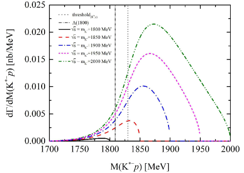
Figure 4: With the integration of the $M_{\mathrm{inv}}(\bar{K}^{0}\pi)$, we present the mass distribution of $(\frac{d\Gamma}{dM_{\mathrm{inv}}(K^{*-}p)})$ with the dependence on $M_{\mathrm{inv}}(K^{*-}p)$, The $(\frac{d\Gamma}{dM_{\mathrm{inv}}(K^{-}p)})$ values obtained with different $\sqrt{s}~{}(\sqrt{s}=m_{K^{+}}+1800,1850,1900,1950,2000~{}\mathrm{MeV})$ values are shown by different lines. And the vertical black dashed line and black dotted line represent the threshold of $M_{K^{*-}p}$ and the boundary of $\Lambda(1800)$, respectively.

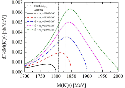
Figure 5: The mass distribution of $(\frac{d\Gamma}{dM_{\mathrm{inv}}(K^{-}p)})$ with the dependence on $M_{\mathrm{inv}}(K^{-}p)$. The labels are same as Fig. 4.

IV Conclusions

We have addressed the study of the $\gamma~{}p\rightarrow pK^{+}K^{*-}(K^{*-}\rightarrow K^{-}\pi^{0})$ and $\gamma~{}p\rightarrow pK^{+}K^{*-}(K^{*-}\rightarrow\bar{K}^{0}\pi^{-})$ plus the $\gamma~{}p\rightarrow pK^{+}K^{-}p$ reaction in search of information for the $\Lambda(1800)$ resonance from the perspective that this resonance is dynamically generated by the interaction of vector-baryon ($1/2^{+}$) in the channel of $\bar{K}^{*}N$ and its coupled channels. In the framework of the chiral unitary approach, where this resonance, among others, is generated, the $\Lambda(1800)$ couples mostly to $\bar{K}^{*}N$. From this perspective we have evaluated the cross sections for photoproduction of this resonance, by looking at $K^{+}K^{*-}p$ production on one side and $K^{+}K^{-}p$ production on the other. Both reactions are complementary and the strength of the cross sections, the shapes in the invariant mass distributions and the dependence on the total energy of the initial $\gamma p$ system, are tied to the picture of this resonance as a molecular state of $\bar{K}^{*}N$ with its coupled channels.

The two reactions chosen, with $K^{+}K^{*-}p$ and $K^{+}K^{-}p$ final states are complementary. In the first one, one detects the $K^{*-}$ from its $\pi^{-}\bar{K}^{0}$ decay channel, and one can go below the nominal $K^{*-}p$ threshold due to the width of the $K^{*-}$. The combination of the phase space, the resonant pole below the $K^{*-}p$ threshold and the mass distribution of the $K^{*-}$, have as a consequence that a peak is still seen above the $K^{*-}p$ threshold, displaced to higher energies than in the case of the $K^{-}p$ final state, where there are no restrictions of phase space and the resonance shows up more clearly in the $K^{-}p$ mass distribution, although the peak is also a bit displaced to higher energies with respect the nominal mass of the resonance.

The features of the two mass distributions, the strength and the $\sqrt{s}$ dependence of the cross sections offer a rich variety of information that can be contrasted with future experiments and should shed light on the nature of this resonance and its analogy to the $\Lambda(1405)$. The results obtained here should provide a motivation to carry on these experiments.

V Acknowledgement

This work is supported by the National Natural Science Foundation of China under Grants and No. 12405089 and No. 12247108 and the China Postdoctoral Science Foundation under Grant No. 2022M720360 and No. 2022M720359.

References

- Tran et al. (1998) M. Q. Tran et al. (SAPHIR), Phys. Lett. B 445, 20 (1998).
- Tovee et al. (1971) D. N. Tovee et al., Nucl. Phys. B 33, 493 (1971).
- Ciborowski et al. (1982) J. Ciborowski et al., J. Phys. G 8, 13 (1982).
- Morelos Pineda et al. (1993) A. Morelos Pineda et al. (E761), Phys. Rev. Lett. 71, 2172 (1993).
- Duryea et al. (1991) J. Duryea et al., Phys. Rev. Lett. 67, 1193 (1991).
- Anisovich et al. (2007) A. V. Anisovich, V. Kleber, E. Klempt, V. A. Nikonov, A. V. Sarantsev, and U. Thoma, Eur. Phys. J. A 34, 243 (2007).
- Wilkinson et al. (1981) C. Wilkinson et al., Phys. Rev. Lett. 46, 803 (1981).
- Paterson et al. (2016) C. A. Paterson et al. (CLAS), Phys. Rev. C 93, 065201 (2016).
- de la Vaissiere et al. (1985) C. de la Vaissiere et al., Phys. Rev. Lett. 54, 2071 (1985), [Erratum: Phys.Rev.Lett. 55, 263 (1985)].
- Goers et al. (1999) S. Goers et al. (SAPHIR), Phys. Lett. B 464, 331 (1999).
- Ablikim et al. (2021) M. Ablikim et al. (BESIII), Phys. Lett. B 814, 136110 (2021).
- Aduszkiewicz et al. (2016) A. Aduszkiewicz et al. (NA61/SHINE), Eur. Phys. J. C 76, 198 (2016).
- Biagi et al. (1981) S. F. Biagi et al., Z. Phys. C 9, 305 (1981).
- Dobbs et al. (2014) S. Dobbs, A. Tomaradze, T. Xiao, K. K. Seth, and G. Bonvicini, Phys. Lett. B 739, 90 (2014).
- Adamova et al. (2017) D. Adamova et al. (ALICE), Eur. Phys. J. C 77, 389 (2017).
- Chien et al. (1966) C. Y. Chien, J. Lach, J. Sandweiss, H. D. Taft, N. Yeh, Y. Oren, and M. Webster, Phys. Rev. 152, 1171 (1966).
- Sarantsev et al. (2019) A. V. Sarantsev, M. Matveev, V. A. Nikonov, A. V. Anisovich, U. Thoma, and E. Klempt, Eur. Phys. J. A 55, 180 (2019).
- Carmony et al. (1964) D. D. Carmony, G. M. Pjerrou, P. E. Schlein, W. E. Slater, and D. H. Stork, Phys. Rev. Lett. 12, 482 (1964).
- Beretvas et al. (1986) A. Beretvas et al., Phys. Rev. D 34, 53 (1986).
- Bardadin-Otwinowska et al. (1975) M. Bardadin-Otwinowska et al., Nucl. Phys. B 90, 397 (1975).
- Ronniger and Metsch (2011) M. Ronniger and B. C. Metsch, Eur. Phys. J. A 47, 162 (2011).
- Adamczewski-Musch et al. (2018) J. Adamczewski-Musch et al. (HADES), Phys. Lett. B 781, 735 (2018).
- Crede (2023) V. Crede (GlueX), Few Body Syst. 64, 32 (2023).
- Abazov et al. (2023) V. Abazov et al. (PANDA) (2023).
- Arellano and Adriazola (2024) H. F. Arellano and N. A. Adriazola, Eur. Phys. J. A 60, 158 (2024).
- Nakamura and Jido (2014) S. X. Nakamura and D. Jido, PTEP 2014, 023D01 (2014).
- Van Cauteren et al. (2004) T. Van Cauteren, D. Merten, T. Corthals, S. Janssen, B. Metsch, H. R. Petry, and J. Ryckebusch, Eur. Phys. J. A 20, 283 (2004).
- Jackson et al. (2015) B. C. Jackson, Y. Oh, H. Haberzettl, and K. Nakayama, Phys. Rev. C 91, 065208 (2015).
- Bernard et al. (1992) V. Bernard, N. Kaiser, J. Kambor, and U. G. Meissner, Phys. Rev. D 46, R2756 (1992).
- Lee (1968) B. W. Lee, Phys. Rev. 170, 1359 (1968).
- Feldman et al. (1961) G. Feldman, P. T. Matthews, and A. Salam, Phys. Rev. 121, 302 (1961).
- Sibirtsev et al. (2006) A. Sibirtsev, J. Haidenbauer, H. W. Hammer, and U. G. Meissner, Eur. Phys. J. A 29, 363 (2006).
- Ellis et al. (2007) J. R. Ellis, A. Kotzinian, D. Naumov, and M. Sapozhnikov, Eur. Phys. J. C 52, 283 (2007).
- Kim et al. (2013) S.-H. Kim, S.-i. Nam, A. Hosaka, and H.-C. Kim, Phys. Rev. D 88, 054012 (2013).
- Kaiser (2005) N. Kaiser, Phys. Rev. C 71, 068201 (2005).
- Ozpineci et al. (2005) A. Ozpineci, S. B. Yakovlev, and V. S. Zamiralov, Mod. Phys. Lett. A 20, 243 (2005).
- Zhong and Zhao (2013) X.-H. Zhong and Q. Zhao, Phys. Rev. C 88, 015208 (2013).
- Quigg and Rosner (1976) C. Quigg and J. L. Rosner, Phys. Rev. D 14, 160 (1976).
- Shi et al. (2023) J. Shi, L.-C. Gui, J. Liang, and G. Liu (2023).
- Yan et al. (2023) B. Yan, C. Chen, and J.-J. Xie, Phys. Rev. D 107, 076008 (2023).
- Dalitz and Tuan (1960) R. H. Dalitz and S. F. Tuan, Annals Phys. 10, 307 (1960).
- Dalitz and Tuan (1959) R. H. Dalitz and S. F. Tuan, Phys. Rev. Lett. 2, 425 (1959).
- Kaiser et al. (1995a) N. Kaiser, P. B. Siegel, and W. Weise, Phys. Lett. B 362, 23 (1995a).
- Kaiser et al. (1995b) N. Kaiser, P. B. Siegel, and W. Weise, Nucl. Phys. A 594, 325 (1995b).
- Oset and Ramos (1998) E. Oset and A. Ramos, Nucl. Phys. A 635, 99 (1998).
- Oller et al. (2000) J. A. Oller, E. Oset, and A. Ramos, Prog. Part. Nucl. Phys. 45, 157 (2000).
- Ecker (1995) G. Ecker, Prog. Part. Nucl. Phys. 35, 1 (1995).
- Bernard et al. (1995) V. Bernard, N. Kaiser, and U.-G. Meissner, Int. J. Mod. Phys. E 4, 193 (1995).
- Oller and Meissner (2001) J. A. Oller and U. G. Meissner, Phys. Lett. B 500, 263 (2001).
- Jido et al. (2003) D. Jido, J. A. Oller, E. Oset, A. Ramos, and U. G. Meissner, Nucl. Phys. A 725, 181 (2003).
- Navas et al. (2024) S. Navas et al. (Particle Data Group), Phys. Rev. D 110, 030001 (2024).
- Oset and Ramos (2010a) E. Oset and A. Ramos, Eur. Phys. J. A 44, 445 (2010a).
- Lutz and Kolomeitsev (2002) M. F. M. Lutz and E. E. Kolomeitsev, Nucl. Phys. A 700, 193 (2002).
- Garcia-Recio et al. (2003) C. Garcia-Recio, J. Nieves, E. Ruiz Arriola, and M. J. Vicente Vacas, Phys. Rev. D 67, 076009 (2003).
- Magas et al. (2005) V. K. Magas, E. Oset, and A. Ramos, Phys. Rev. Lett. 95, 052301 (2005).
- Ikeda et al. (2012) Y. Ikeda, T. Hyodo, and W. Weise, Nucl. Phys. A 881, 98 (2012).
- Guo and Oller (2013) Z.-H. Guo and J. A. Oller, Phys. Rev. C 87, 035202 (2013).
- Mai and Meißner (2015) M. Mai and U.-G. Meißner, Eur. Phys. J. A 51, 30 (2015).
- Roca and Oset (2013a) L. Roca and E. Oset, Phys. Rev. C 87, 055201 (2013a).
- Roca and Oset (2013b) L. Roca and E. Oset, Phys. Rev. C 88, 055206 (2013b).
- Cieplý et al. (2016) A. Cieplý, M. Mai, U.-G. Meißner, and J. Smejkal, Nucl. Phys. A 954, 17 (2016).
- Cieply and Smejkal (2012) A. Cieply and J. Smejkal, Nucl. Phys. A 881, 115 (2012).
- Kamiya et al. (2016) Y. Kamiya, K. Miyahara, S. Ohnishi, Y. Ikeda, T. Hyodo, E. Oset, and W. Weise, Nucl. Phys. A 954, 41 (2016).
- Hyodo and Weise (2008) T. Hyodo and W. Weise, Phys. Rev. C 77, 035204 (2008).
- Révai (2018) J. Révai, Few Body Syst. 59, 49 (2018).
- Bruns and Cieplý (2020) P. C. Bruns and A. Cieplý, Nucl. Phys. A 996, 121702 (2020).
- Miyahara and Hyodo (2018) K. Miyahara and T. Hyodo, Phys. Rev. C 98, 025202 (2018).
- Hyodo and Jido (2012) T. Hyodo and D. Jido, Prog. Part. Nucl. Phys. 67, 55 (2012).
- Meißner (2020) U.-G. Meißner, Symmetry 12, 981 (2020).
- Moriya et al. (2013a) K. Moriya et al. (CLAS), Phys. Rev. C 87, 035206 (2013a).
- Moriya et al. (2013b) K. Moriya et al. (CLAS), Phys. Rev. C 88, 045201 (2013b), [Addendum: Phys.Rev.C 88, 049902 (2013)].
- Schumacher and Moriya (2013) R. A. Schumacher and K. Moriya, Nucl. Phys. A 914, 51 (2013).
- Bando et al. (1985) M. Bando, T. Kugo, S. Uehara, K. Yamawaki, and T. Yanagida, Phys. Rev. Lett. 54, 1215 (1985).
- Bando et al. (1988) M. Bando, T. Kugo, and K. Yamawaki, Phys. Rept. 164, 217 (1988).
- Meissner (1988) U. G. Meissner, Phys. Rept. 161, 213 (1988).
- Nagahiro et al. (2009) H. Nagahiro, L. Roca, A. Hosaka, and E. Oset, Phys. Rev. D 79, 014015 (2009), eprint 0809.0943.
- Bramon et al. (1992) A. Bramon, A. Grau, and G. Pancheri, Phys. Lett. B 283, 416 (1992).
- Oset et al. (2003) E. Oset, J. R. Pelaez, and L. Roca, Phys. Rev. D 67, 073013 (2003).
- Oset et al. (2008) E. Oset, J. R. Pelaez, and L. Roca, Phys. Rev. D 77, 073001 (2008).
- Oset and Ramos (2010b) E. Oset and A. Ramos, Eur. Phys. J. A 44, 445 (2010b).
- Garzon and Oset (2012) E. J. Garzon and E. Oset, Eur. Phys. J. A 48, 5 (2012).
- Mandl and Shaw (1985) F. Mandl and G. Shaw, QUANTUM FIELD THEORY (1985).
- Gamermann et al. (2010) D. Gamermann, J. Nieves, E. Oset, and E. Ruiz Arriola, Phys. Rev. D 81, 014029 (2010).