Diffusion-based RGB-D Semantic Segmentation with Deformable Attention Transformer

Abstract

Vision-based perception and reasoning is essential for scene understanding in any autonomous system. RGB and depth images are commonly used to capture both the semantic and geometric features of the environment. Developing methods to reliably interpret this data is critical for real-world applications, where noisy measurements are often unavoidable. In this work, we introduce a diffusion-based framework to address the RGB-D semantic segmentation problem. Additionally, we demonstrate that utilizing a Deformable Attention Transformer as the encoder to extract features from depth images effectively captures the characteristics of invalid regions in depth measurements. Our generative framework shows a greater capacity to model the underlying distribution of RGB-D images, achieving robust performance in challenging scenarios with significantly less training time compared to discriminative methods. Experimental results indicate that our approach achieves State-of-the-Art performance on both the NYUv2 and SUN-RGBD datasets in general and especially in the most challenging of their image data. Our project page will be available at https://diffusionmms.github.io/

I Introduction

Semantic segmentation represents the challenging problem of assigning a class label to each pixel of an image and corresponds to an essential step in visual scene understanding. Linking the correct subsets of pixels to the correct class, ensuring that pixels around a certain object are not erroneously linked to its class, and dealing with challenging textures or light conditions represent persistent challenges in computer vision and robotics. Accordingly, a body of work has focused on this problem, with the most prominent and high-performance methods currently relying on deep learning techniques with diverse architectures [1, 2, 3, 4, 5, 6, 7, 8]. Among the most recent approaches to the problem is that of combining multimodal sensor data with the hope of achieving improved overall performance and robustness.

Combining information from various sensors equips robots with more resilient capabilities while working in complex environments since each modality can complement the weaknesses of the others. Current multimodal approaches for semantic segmentation typically use a simple dual-branch encoder-decoder architecture, with one branch being used for feature extraction from the RGB modality and the other for auxiliary modality feature extraction.

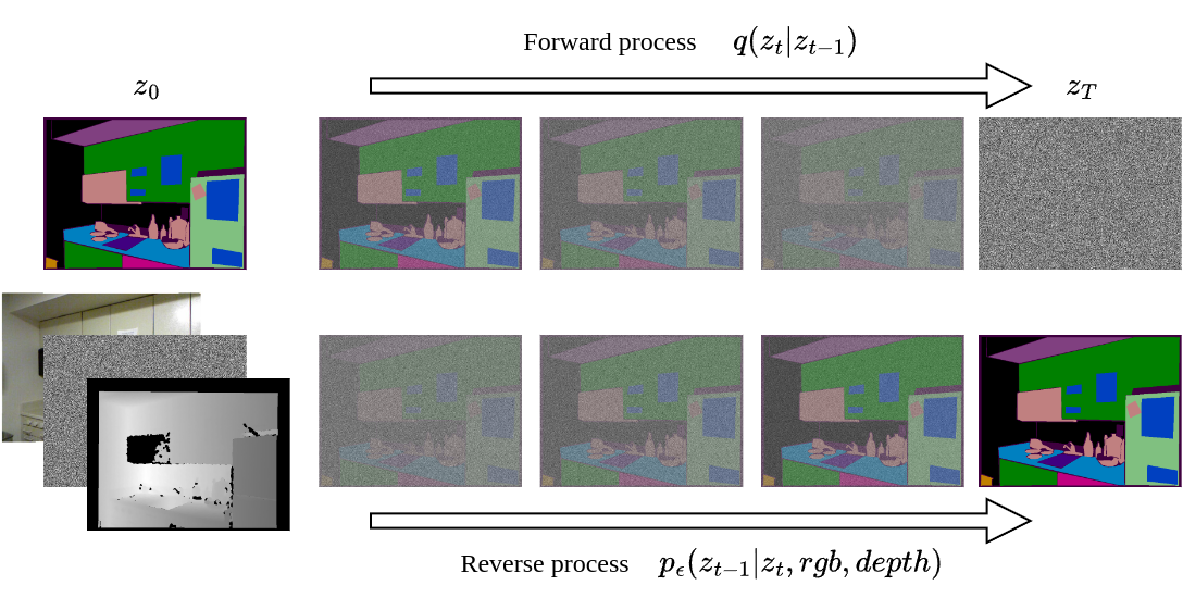
Figure 1: We formulate the RGB-D semantic segmentation task as a denoising diffusion process conditioned by RGB and depth images.

The segmentation mask is then achieved by merging the multimodal information using sophisticated fusion approaches. There are two main fusion schemes that are popular in recent works: interaction-based fusion [9, 5] and exchange-based fusion [1, 10].

Despite being straightforward, these kinds of methods often suffer performance degradation due to many invalid measurements from depth sensors (e.g., caused by stereo disparity errors, the effect of reflective surfaces, and other phenomena). To mitigate this, many methods exploit information from the corresponding RGB image to interpolate these missing values using the colorization method [11], or the HHA image algorithm [12]. However, this step not only adds an additional computational cost but also compromises the integrity of how reality is captured.

Furthermore, to the best of the authors’ knowledge, all methods on RGB-D semantic segmentation only employ the discriminative-based paradigm [5, 9, 1, 10]. Recently, generative-based methods such as diffusion models have been shown to achieve impressive results on several vision tasks. Although diffusion was originally designed for the image generation problem, many efforts have been made to apply it to RGB semantic segmentation [13, 14, 15].

Motivated by its potential, in this paper we introduce a general, simple, yet effective diffusion framework for high-performance RGB-D semantic segmentation, overcoming several of the identified challenges in the domain. In summary, our contributions are as follows: First, we demonstrate that using a deformable transformer as an image encoder in a discriminative-based architecture can alleviate the problem caused by invalid pixels in depth images. Second, we demonstrate that the use of diffusion can achieve improved results - compared to the State-of-the-Art (SOTA) - combined with reduced training time. Third, experimental results demonstrate that our method achieves SOTA on both the NYUv2 and SUNRGBD datasets and several challenging setups.

The remainder of this paper is organized as follows. Section II presents related work, while the proposed method is detailed in Section III. Evaluation studies are shown in Section IV, while conclusions are drawn in Section V.

II Related work

This work relates to the body of literature on RGB-D semantic segmentation alongside the works considering the role of diffusion in image segmentation in general.

II-A RGB-D Semantic Segmentation

An emerging trend for improving performance in RGB-D semantic segmentation is to create methods that enhance the 2D representation of RGB-D images. Designing complex fusion mechanisms to better utilize features extracted from both domains has become a de facto approach in the field. Most methods can be categorized into two main strategies.

First, this relates to the interaction-based fusion strategy which focuses on integrating features from different modalities through direct interaction, typically via cross attention, or feature concatenation operations. The information from the two modalities can be merged directly at the input level through channel-wise averaging or concatenation and then processed by a single stream network as described in [16, 17, 18, 19]. Despite its simplicity, merging raw data from different modalities too early can lead to a loss of modality-specific features, limited cross-modal interactions, increased sensitivity to noise and incomplete data. This approach lacks adaptability, contextual understanding, and often results in suboptimal performance, especially in complex scenarios. Another set of works proposed a fusion mechanism at the feature level which combines information from different modalities after extracting rich features separately from each modality. Zhang et al [9] introduced a feature rectification module to refine features between modalities and a feature fusion module to enable the comprehensive exchange of long-range contexts before final fusion. Ying et al [20] suggest that using depth map uncertainty as an auxiliary signal can enhance segmentation accuracy and robustness. Yin et al [5] suggest an attention-based fusion scheme and performing supervised RGB-D pre-training on ImageNet-1K to develop a more effective backbone network for downstream tasks.

Second, the exchange-base fusion strategy involves the exchange of information between modalities through shared representations. The idea is to dynamically refine features from each modality based on insights gained from the other. TokenFusion [10] employs the prune-then-substitute scheme to replace uninformative tokens with more valuable ones from the other modality. This work is studied further by Jia et al [1], where it is suggested that the risk of all tokens engaging in unnecessary exchange can lead to significant information loss, and proposing an exchange-based strategy based on cross-modal transformers instead.

II-B Diffusion in Image Segmentation

All current literature in the field of RGB-D semantic segmentation follows the discriminative paradigm which broadly represents the community standard for semantic segmentation. However, recently generative models have taken the community by storm with their remarkable performance in the image generation task. Several studies suggest that generative models can achieve promising results on segmentation tasks [14, 15, 13]. Baranchuk et al [13] illustrated that feature representations learned from pre-trained diffusion models can be fine-tuned for the segmentation task and achieve SOTA results with limited labels. In [15], Chen et al demonstrated a general framework based on diffusion models for panoptic segmentation on images and videos. In [14], Ji et al proposed a diffusion-based architecture that is suitable for several visual dense prediction tasks including semantic segmentation, depth estimation, and BEV map segmentation. These results are based on RGB image data. Their promising results in combination with the benefits of multi-modality motivated the incorporation of diffusion in the proposed architecture for RGB-D semantic segmentation.

III Proposed Method

III-A Preliminaries

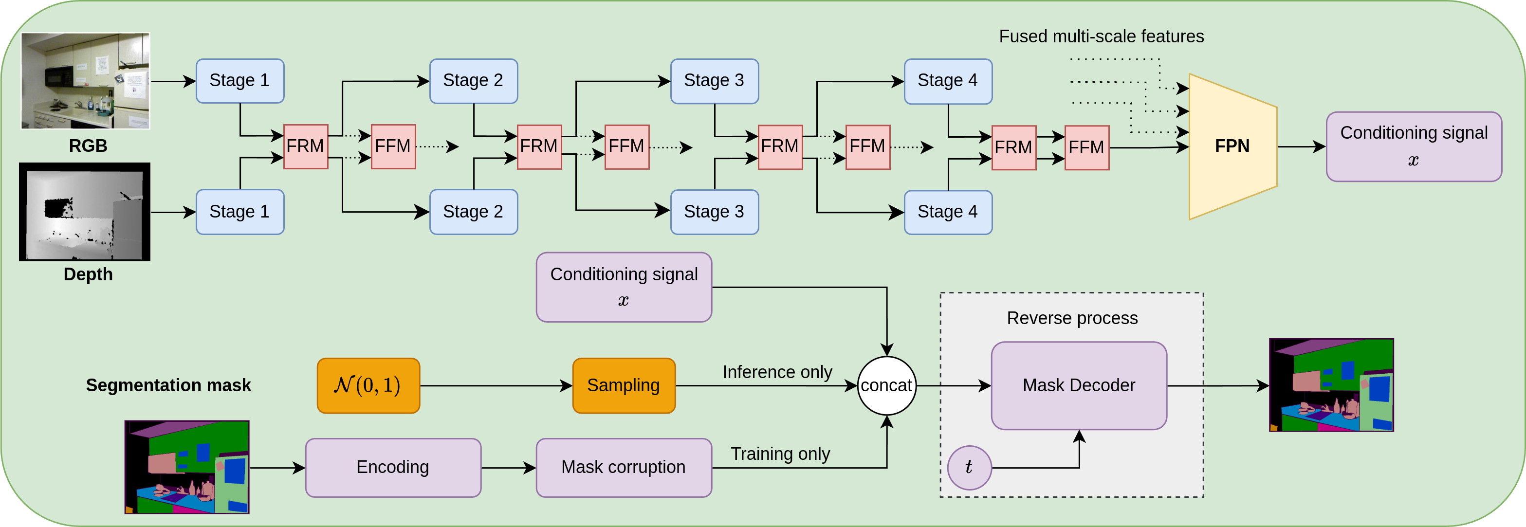
Figure 2: The architecture of our RGBD semantic mask generation framework. A Deformable Attention Transformer is used as the hierarchical encoder to extract features from RGB and depth images. Multi-scale features from both branches are then processed using fusion modules followed by a Feature Pyramid Network to create a conditioning signal $x$ that matches the shape of the noisy segmentation ground-truth. A deformable attention mask encoder is trained to gradually denoise the concatenated signal to generate the segmentation mask.

III-A1 Deformable Attention Transformer

We first revisit the vanilla Vision Transformer with the attention mechanism at its heart. Given an input feature vector $x\in\mathbb{R}^{N\times C}$, a M heads Multi-Head Self-Attention (MHSA) block is defined as

$$q = W_{q}x,~{}k=W_{k}x,~{}v=W_{v}x$$ (1)

$$z_{m} = \textrm{softmax}(q_{m}k_{m}^{\top}/\sqrt{d})v_{m}$$ (2)

$$z = \textrm{concat}(z_{1},...,z_{M})W_{out}$$ (3)

where $W_{out},W_{q},W_{k},W_{v}$ are projection matrices, $d$ represents the dimension of each head, $z_{m}$ represents the output embedding of the $m$-th attention head, and $q_{m},k_{m},v_{m}\in\mathbb{R}^{N\times d}$ represent query, key, and value embeddings respectively.

Many attempts have been made to address the quadratic complexity with respect to input dimension in the vanilla Vision Transformer [21, 22, 23, 24]. The Deformable Attention Transformer [23, 24] introduces the idea of learning a few sets of sampling offsets, shared across all queries, to adjust keys and values to important regions, based on the observation that global attention typically produces similar patterns for various queries [25, 26]. By doing that, it effectively captures relationships between tokens by focusing on key areas of the feature map. Given the initial attention region position $p$, it is dynamically updated through deformable sampling points learned from queries via offset networks $\Delta p=\epsilon_{offset}(q)$. The features are sampled at the locations of deformed points via a bilinear interpolation function $\varphi$. They serve as keys and values, transformed by projection matrices.

$$q = W_{q}x,\bar{k}=W_{k}\bar{x},\bar{v}=W_{v}\bar{x}$$ (4)

$$\Delta p = \epsilon_{\textrm{offset}}(q),\bar{x}=\varphi(x;p+\Delta p)$$ (5)

where $\bar{k},\bar{v}$ respectively denotes the deformed key and value embeddings. More details can be found in [23, 24].

III-A2 Diffusion models

Diffusion models [27, 28] are generative models that can learn the underlying data distribution, allowing one to synthesize new data points from pure noise. They consist of two processes. In the forward process, noise is iteratively added to the data sample $z_{0}$, converting it into a latent noisy sample $z_{t}$ based on a noise scheduler $\beta_{s}$ [28, 27]. The whole process is mathematically defined as

$$q(z_{t}|z_{0})=\mathcal{N}(z_{t};\sqrt{\bar{\alpha}_{t}}z_{0},(1-\bar{\alpha}_{t}I)),t\in{0,1,...,T}$$ (6)

where $\bar{\alpha}_{t}=\prod_{s=0}^{t}(1-\beta_{s})$, $I$ is the identity matrix.

One can control the output of diffusion models to generate samples belonging to a domain of interest simply by concatenating a conditioning signal $x$ to the noisy sample $z_{t}$. In the training stage, a neural network $f_{\epsilon}(z_{t},x,t)$ is trained to predict $z_{0}$ from $z_{t}$ given the conditioning signal $x$ by optimizing a training objective function. In the inference stage, starting from a sample of noise $z_{T}$, the data sample $z_{0}$ is generated by applying the model $f_{\epsilon}$ iteratively with transition rules such as ones described in [27, 28].

III-B Proposed architecture

We start by considering the method described in [9] as the baseline. In [9], Zhang et al proposed a sophisticated fusion module to facilitate interactions between RGB and depth images. However, in order to achieve good results, it relies on the three-channel HHA encoding [12] of the depth images. To understand the underlying challenges of the method, we retrained their models on raw depth images with a high number of invalid pixels which can be up to over 80% the total number of pixels in a depth image and found that the training loss contains multiple spikes (see Figure 3) suggesting training instability and possible overfiting to the noise in the depth images. We argue that instead utilizing the Deformable Attention Transformer (DAT) as the encoder – with its characteristic of having the adaptive spatial aggregation conditioned by input and task information [29]– is well suited to tackle the challenge posed by the invalid pixels in depth images. Furthermore, a diffusion model, as a denoising process, is advantageous when learning the underlying distribution of depth images given their nature of having uncertain measurements.

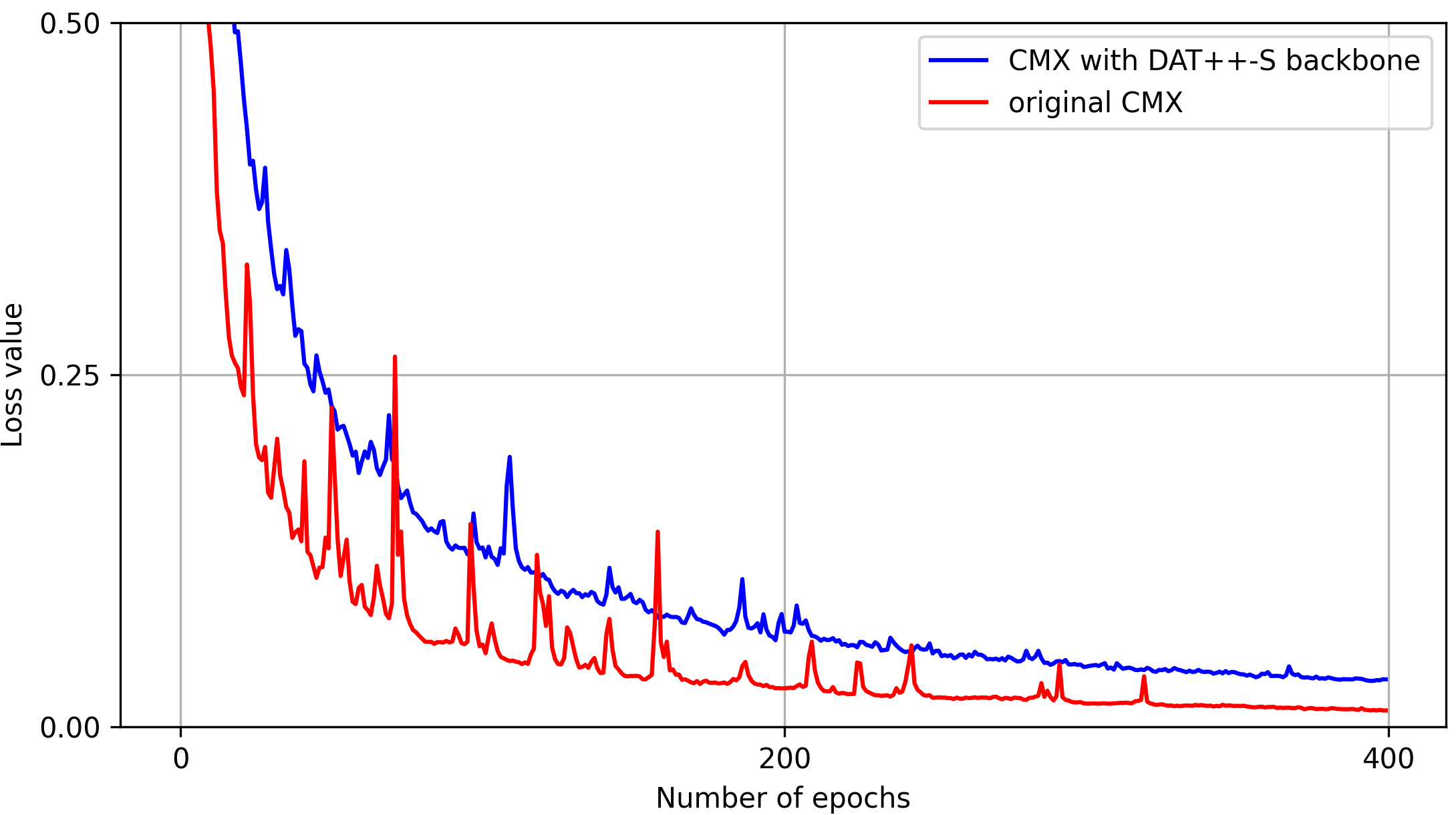
Figure 3: Loss comparison between training the original CMX [9] model and when using DAT++-S as encoder on raw depth images.

Accordingly, we formulate the RGB-D semantic segmentation task as a conditioning image generation task. The goal is to learn the underlying distribution of the segmentation mask conditioned by RGB and depth images. In inference time, noise sampled from a normal distribution is concatenated with fusion features extracted from RGB-D inputs via a deformable attention transformer used as an encoder. The combined signal then goes through the reverse process to iteratively generate the final segmentation mask given the RGB-D inputs. The overall architecture of our method is illustrated in Figure 2. In the following sections, the details of each component in the architecture are presented.

III-B1 Encoder

The double encoder architecture is used to obtain the conditioning signal from paired RGB-D frames. We employ the DAT described in [24] as the encoder to extract multi-scale features at different resolutions from both modalities. We use the feature rectification modules (FRM) and feature fusion module (FFM) described in [9] to obtain multi-scale RGB-D fusion features. Notice that the output of the conditioning signal should be of the same size as the segmentation ground-truth. To reduce computation cost for the mask decoder, we resize the segmentation mask from $h\times w$ to $\frac{h}{4}\times\frac{w}{4}$. Accordingly, we generate the conditioning signal of shape $256\times\frac{h}{4}\times\frac{w}{4}$ by merging multi-scale RGB-D fusion features via a Feature Pyramid Network (FPN) and then aggregating the output using a $1\times 1$ convolution.

III-B2 Mask Decoder

The mask decoder $f_{\epsilon}$ takes the noisy mask $y_{t}$ and the conditioning signal via concatenation as input. It is then trained to reconstruct the segmentation groundtruth with the original size using the standard cross entropy loss for the semantic segmentation task. Following [14], we form the mask decoder by stacking six layers of deformable attention blocks [30] with time embedding.

III-B3 Training

During training, we first perform the forward process which converts the segmentation label $y$ into the noisy map $y_{t}$ and then train the reverse model to learn how to remove noise. The training procedure is outlined in Algorithm 1. Details about components in the forward process are presented below:

Label encoding. Diffusion models were originally designed to work with continuous data and Gaussian noise. Several studies have investigated ways to apply diffusion to tasks with discrete labels [31, 15, 14] such as semantic segmentation. Inspired by the work of Ji et al [14], we use the class embedding approach in which a learnable embedding layer is used to project discrete labels into a high-dimensional space, normalized by a sigmoid function. The encoded labels are scaled to the range of $[-s,s]$ as shown in Algorithm 1.

Mask Corruption. The Gaussian noise is added to the encoded segmentation ground truth to produce the noise mask $y_{t}$. The magnitude of noise to be added is regulated by $\alpha_{t}$, which follows a decreasing pattern over the timesteps $t\in[0,1]$. Various noise schedules, such as cosine [32] and linear schedules [27], are analyzed in Section IV.

Algorithm 1 Training procedure

⬇

def train(rgb, depth, mask):

# obtain fused features

rgb_enc = rgb_encoder(rgb) #DAT encoder

depth_enc = depth_encoder(depth)#DAT encoder

fused = fusion(rgb_enc, depth_enc)# CMX based

# encode segmentation mask

mask_enc = encoding(mask)

mask_enc = (sigmoid(mask_enc) * 2 - 1) * s

# noisify gt

t, eps = uniform(0, 1), normal(mean=0, std=1)

mask_noise = sqrt(alpha_bar(t)) * mask_enc + sqrt(1 - alpha_bar(t))*eps

# predict and calculate loss

mask_pred = mask_decoder(mask_noise,fused,t)

loss = cross_entropy(mask_pred, mask)

return loss

III-B4 Inference

The inference process is outlined in Algorithm 2. Given paired RGB and depth images as the conditional inputs, the model begins with a random noise map generated from a Gaussian distribution and progressively improves the prediction. To minimize the number of iterative steps, we choose the DDIM update rule [28, 14] for the sampling process. The key hyperparameter in this update rule is the time difference td which determines how far apart consecutive timesteps are chosen during the reverse diffusion process. Larger time gaps between steps allow for faster sampling at the potential cost of sample quality. Our experiments show that td$~{}=1$ and the number of steps of 3 work best for our method. The details of the DDIM update rule is presented in Algorithm 3.

Algorithm 2 Sampling procedure

⬇

def sampling(rgb, depth, steps, td=1):

# obtain fused features

rgb_enc = rgb_encoder(rgb) #DAT encoder

depth_enc = depth_encoder(depth)#DAT encoder

fused = fusion(rgb_enc, depth_enc)# CMX based

# sample noise

mask_t = normal(0, 1)

for step in range(steps):

# get time intervals

t_now = 1 - step / steps

t_next = max(1 - (step + 1 + td) / steps, 0)

# predict mask_0 from mask_t

mask_pred = mask_decoder(mask_t,fused,t_now)

# estimate mask_t at t_next

mask_t = ddim_step(mask_t, mask_pred, t_now, t_next)

return mask_pred

Algorithm 3 DDIM update rule

⬇

def alpha_bar(t, ns=0.0002, ds=0.00025):

"""cosine noise scheduler"""

n = torch.cos((t+ns)/(1+ds) * math.pi/2)**-2

return -torch.log(n - 1, eps=1e-5)

def ddim_step(mask_t,mask_pred,t_now,t_next):

"""estimate x with DDIM update rule."""

$\alpha_{now}$ = alpha_bar(t_now)

$\alpha_{next}$ = alpha_bar(t_next)

mask_enc = encoding(mask_pred)

mask_enc = (sigmoid(mask_enc) * 2 - 1) * s

eps = $\frac{1}{\sqrt{1-\alpha_{now}}}$*(mask_t -$\sqrt{\alpha_{now}}$* mask_enc)

mask_next =$\sqrt{\alpha_{next}}$* mask_enc +$\sqrt{1-\alpha_{now}}$*eps

return mask_next

IV Experimental Evaluation

IV-A Experimental setup

IV-A1 Datasets and Metrics

We test our method on the validation sets of two popular RGB-D datasets: NYUv2 [33] and SUN-RGBD [34]. For the NYUv2 dataset, which has 40 labeled classes, we follow the standard split of 795 training and 654 testing images. The SUN-RGBD dataset is seven times larger than the NYUv2 dataset in size, containing 5285 training and 5050 testing images with 37 labeled classes. To evaluate the performance of our method, we use the standard mean intersection over union (meanIoU) metric [35] for the semantic segmentation task.

IV-A2 Training details and hyperparameters

For all experiments, we train our models using the AdamW optimizer [36], with an initial learning rate of $6\times 10^{-5}$ and a weight decay of 0.01. The learning rate is regulated using the warmup polynomial decay scheduler. As seen in many previous works [9, 20, 5], the discriminative paradigm needs at least 300 to 500 epochs to obtain good results on both NYUv2 and SUN-RGBD datasets. We found that our diffusion-based model can converge in significantly less amount of time. We train the NYUv2 and SUN-RGBD datasets for 100 and 50 epochs, respectively. For data augmentation, we perform resize, random crop, and random flip operations on both RGB and depth images.

IV-A3 Ablation on architectures

Figure 4 depicts reference sampling points learned by the offset network in the Deformable Attention Transformer encoder. For each attention module, reference points are initially created as uniform grids that remain consistent across the input data. An offset network then processes all query features to generate corresponding offsets for these reference points. They guide the candidate keys/values toward important regions, enhancing the original self-attention module with greater flexibility and efficiency to capture more important features. It can be seen in Figure 4 that the learned reference points are shifted towards salient regions in the depth image, including the large invalid region covering the microwave in the RGB image. By avoiding the discontinuous transition between valid and invalid regions, the model can perceive the invalid regions as a whole object instead of overfitting to noisy measurements in the depth image. This insight might hold true for invalid regions caused by other reflective surfaces such as television screens or windows suggesting that DAT, with its data-dependent characteristic, can effectively exploit depth features even under severe uncertainty measurements.

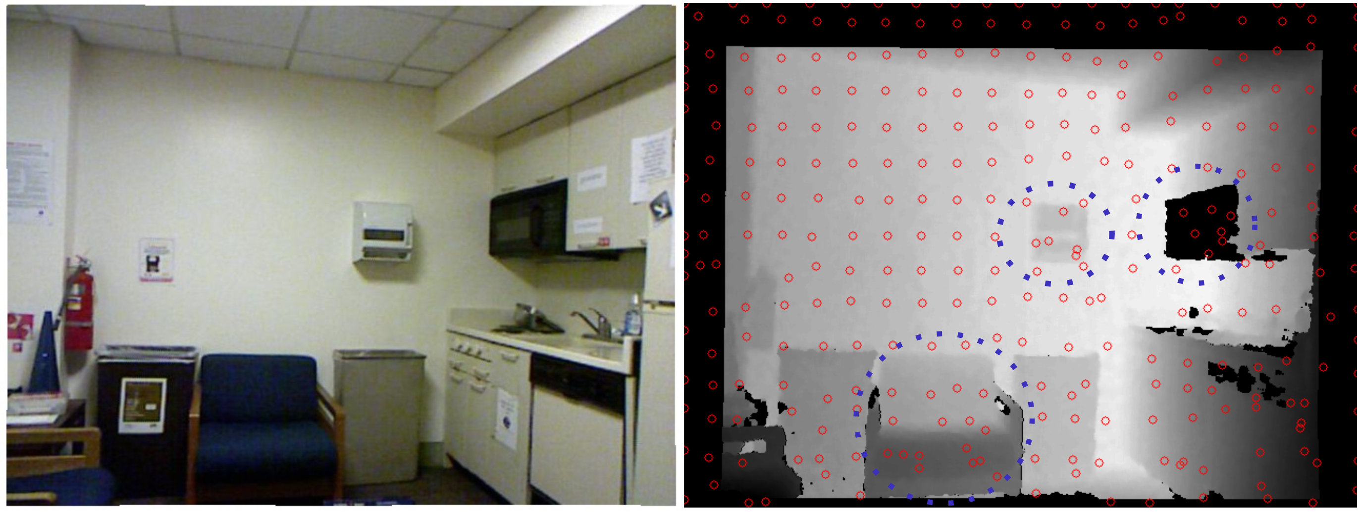
Figure 4: Reference sampling points

The superiority of DAT on RGB-D semantic segmentation over other non data-dependent encoders such as MixTransformer [37] is quantitatively shown in Table I. We take the result reported in [9] as the baseline. By simply changing the encoder of the model to DAT++-S [24], we achieved 3.3% meanIoU boost in the NYUv2 dataset as seen in Table I. However, when evaluating a larger dataset like SUN-RGBD using the discriminative model, we did not achieve any performance boost. By using the diffusion model as the alternating paradigm, we achieved better results compared to the discriminative model on both datasets as seen in Table I while spending significantly less time/epochs to train.

TABLE I: Performance comparison between DAT++ and MiT-B5 using different paradigms on NYUv2 and SUN-RGBD dataset

Methods	NYUv2	SUN-RGBD
CMX (MiT-B5)	56.9	52.4
Discriminative-based (DAT++-S[24])	60.2	52.4
Diffusion-based (DAT++-S[24])	61.2	53.7

IV-A4 Evaluation results on challenging datasets

We evaluate our diffusion based framework using 3 encoder variants namely DAT++-T, DAT++-S, DAT++-B [24]. They achieve SOTA results compared to current literature in the field as shown in Table II. On the NYUv2 dataset, our method with the DAT++-S encoder achieves the best meanIoU of 61.2% which is the number one on the dataset leaderboard at the time of writing. Interestingly, increasing the model size to DAT++-B leads to 0.4% performance drop. This might be the overfitting problem when using a large model on a small dataset like NYUv2 dataset. On the SUN-RGBD dataset, we achieved the best result of 53.9% with DAT++-B encoder. We lose only to GeminiFusion with Swin-Large encoder (197M parameters) which is much larger than DAT++-B encoder (94M parameters). Therefore, our method remains the best method performing on the SUN-RGBD dataset compared with other similar size models. Furthermore, when we evaluate on the SUN-RGBD dataset using the model trained on NYUv2 dataset and vice versa, we observe only a modest performance drop for all variants of our model, which suggests a good generalization capability of our method.

TABLE II: Comparison with other State-of-the-art methods on the NYUv2 and SUN-RGBD datasets. Red numbers indicate the results when evaluating SUN-RGBD dataset using the model trained on NYUv2 and vice versa. The scale value $s=0.01$

Methods	NYUv2	SUN-RGBD
CMX (MiT-B4)[9]	56.3	52.1
CMX (MiT-B5)[9]	56.9	52.4
DFormer-S[5]	53.6	50.0
DFormer-B[5]	56.9	51.2
DFormer-L[5]	57.2	52.5
TokenFusion	54.2	52.4
GeminiFusion (MiT-B3)[1]	56.8	52.7
GeminiFusion (MiT-B5)[1]	57.7	53.3
GeminiFusion (Swin-L)[1]	60.9	54.6
Ours (DAT++-T)	59.7 (59.7)	52.6 (50.6)
Ours (DAT++-S)	61.2 (61.1)	53.7 (51.2)
Ours (DAT++-B)	60.8 (60.4)	53.9 (51.4)

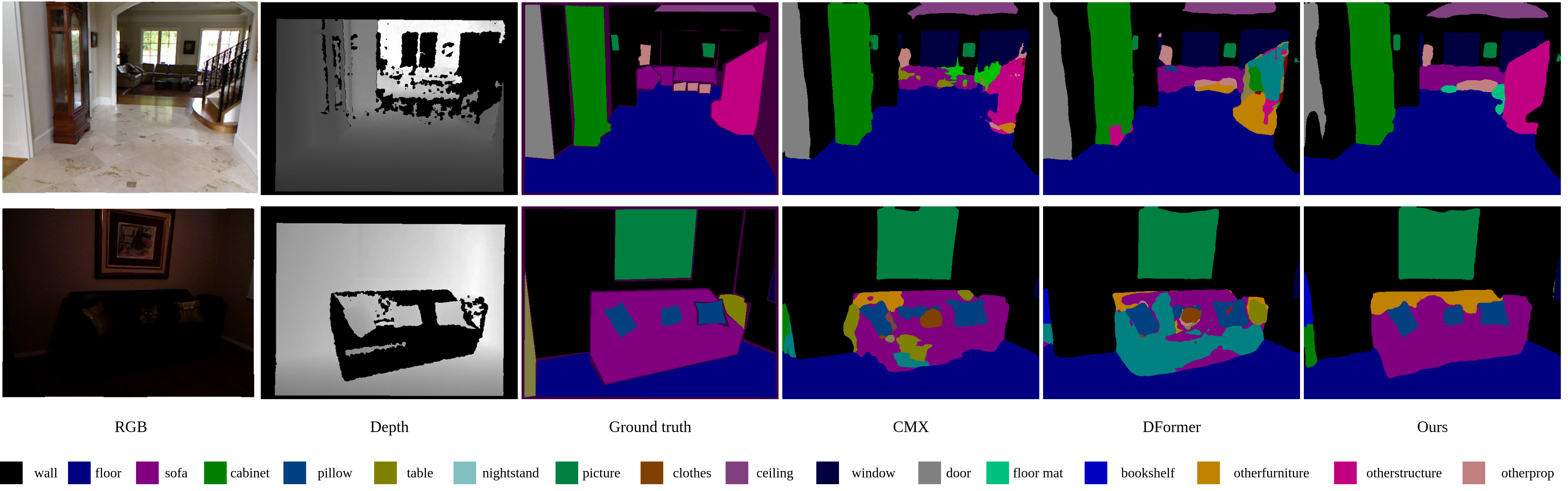
Figure 5: Our segmentation results show that our method has better understanding of invalid depth regions than other methods in both normal (upper row) and low-light conditions (lower row)

TABLE III: Comparison with other methods on challenging subsets. The red numbers indicate the relative performance drop compared with evaluation results on original datasets. DAT++-S is used as the encoder

Datasets	Methods	Nominal	Low-light	Invalid	Small
NYUv2	CMX (MiT-B2)[9]	54.1	50.6 (3.5)	52.8 (1.3)	49.2 (4.9)
	DELIVER[38]	56.3	53.8 (2.5)	51.8 (4.5)	48.5 (7.8)
	DFormer-B[5]	55.6	52.8 (2.8)	51.5 (4.1)	50.4 (5.2)
	DFormer-L[5]	57.2	53.6 (3.6)	53.1 (4.1)	51.6 (5.6)
	Ours (s=0.01)	61.2	58.8 (2.4)	59.3 (1.9)	56.6 (4.6)
	Ours (s=0.03)	61.5	58.9 (2.6)	58.7 (2.8)	56.6 (4.9)
SUN-RGBD	DFormer-B	51.2	46.4 (4.8)	43.2 (8.0)	43.8 (8.0)
	DFormer-L	52.5	47.3 (5.2)	43.2 (8.3)	45.1 (7.4)
	Ours (s=0.01)	53.7	52.2 (1.5)	48.2 (5.5)	49.0 (4.7)
	Ours (s=0.03)	53.8	52.3 (1.5)	47.8 (6.0)	49.0 (4.8)

To further demonstrate the capacity of our method to exploit depth features under heavy uncertainty, we conduct further evaluations on three focused of sub-datasets, namely

• Most invalid pixels: We sort the NYUv2 and SUN-RGBD datasets based on the percentage of invalid pixels in the depth images. We take the subset of the top 20% depth images with the highest percentage of invalid pixels. We call this the ‘invalid’ dataset.

• Low light: For each paired RGB-D frame in the original datasets, we deliberately decrease the intensity of the RGB images using gamma correction operation. The intensity of a normalized image $I$ is adjusted based on the formula $I_{dark}=I^{\gamma},\gamma=2$. We call this the ‘low-light’ subset of the dataset.

• Small objects: We ignore some labels in the ground truth which are less affected by noisy depth data and only evaluate the meanIoU metric of the rest. For NYUv2, we ignore the [“wall”, “floor”, “ceiling”, “otherstructure”, “otherfurniture”, “otherprop”] labels. For SUN-RGBD, we ignore the [“wall”, “floor”, “ceiling”] labels. We call this the ‘small’ objects dataset.

Table III shows that our method outperforms others across all three challenging datasets, with less performance drop. This proves its effectiveness in modeling RGB-D images, even with a high percentage of invalid depth pixels. Qualitative results are shown in Figure 5

IV-A5 Ablation study

We conduct ablation experiments to find the best value for several key hyperparameters in diffusion models. Table IV shows that using cosine schedule achieves slightly better results than linear schedule.

TABLE IV: Ablation study on different noise schedules with DAT++-S and scale value $s=0.01$.

Scheduler	NYUv2	SUN-RGBD
cosine	61.2	53.7
linear	60.9	53.6

Table V shows that 0.03 and 0.001 are the best scale value for NYUv2 and SUN-RGBD dataset respectively. It is noted that $s=0.01$ and $s=0.03$ work well for both datasets, whereas $s=0.001$ improves the performance on SUN-RGBD by a small margin but disproportionally worsens the results on the NYUv2 dataset.

TABLE V: Ablation study on different scale values with DAT++-S

Scale	NYUv2	SUN-RGBD
0.001	58.1	54.0
0.01	61.2	53.7
0.03	61.5	53.8
0.05	60.8	53.3
0.1	60.7	53.2

V Conclusion

Our diffusion-based framework improves RGB-D semantic segmentation and the use of the Deformable Attention Transformer for depth feature extraction robustifies handling invalid depth regions. Experiments on NYUv2 and SUN-RGBD show State-of-the-Art performance with greater efficiency and reduced training time, underscoring the potential of generative models for more accurate vision-based reasoning in autonomous systems.

References

- [1] D. Jia, J. Guo, K. Han, H. Wu, C. Zhang, C. Xu, and X. Chen, “Geminifusion: Efficient pixel-wise multimodal fusion for vision transformer,” arXiv preprint arXiv:2406.01210, 2024.
- [2] J. Jiang, L. Zheng, F. Luo, and Z. Zhang, “Rednet: Residual encoder-decoder network for indoor rgb-d semantic segmentation,” arXiv preprint arXiv:1806.01054, 2018.
- [3] H. Zhao, J. Shi, X. Qi, X. Wang, and J. Jia, “Pyramid scene parsing network,” in Proceedings of the IEEE conference on computer vision and pattern recognition, 2017, pp. 2881–2890.
- [4] O. Ronneberger, P. Fischer, and T. Brox, “U-net: Convolutional networks for biomedical image segmentation,” in Medical image computing and computer-assisted intervention–MICCAI 2015: 18th international conference, Munich, Germany, October 5-9, 2015, proceedings, part III 18. Springer, 2015, pp. 234–241.
- [5] B. Yin, X. Zhang, Z. Li, L. Liu, M.-M. Cheng, and Q. Hou, “Dformer: Rethinking rgbd representation learning for semantic segmentation,” 2024.
- [6] X. Hu, K. Yang, L. Fei, and K. Wang, “Acnet: Attention based network to exploit complementary features for rgbd semantic segmentation,” in 2019 IEEE international conference on image processing (ICIP). IEEE, 2019, pp. 1440–1444.
- [7] L.-Z. Chen, Z. Lin, Z. Wang, Y.-L. Yang, and M.-M. Cheng, “Spatial information guided convolution for real-time rgbd semantic segmentation,” IEEE Transactions on Image Processing, vol. 30, pp. 2313–2324, 2021.
- [8] Z. Wu, G. Allibert, F. Meriaudeau, C. Ma, and C. Demonceaux, “Hidanet: Rgb-d salient object detection via hierarchical depth awareness,” IEEE Transactions on Image Processing, vol. 32, pp. 2160–2173, 2023.
- [9] J. Zhang, H. Liu, K. Yang, X. Hu, R. Liu, and R. Stiefelhagen, “Cmx: Cross-modal fusion for rgb-x semantic segmentation with transformers,” 2023.
- [10] Y. Wang, X. Chen, L. Cao, W. Huang, F. Sun, and Y. Wang, “Multimodal token fusion for vision transformers,” 2022. [Online]. Available: https://arxiv.org/abs/2204.08721
- [11] A. Levin, D. Lischinski, and Y. Weiss, “Colorization using optimization,” ACM Transactions on Graphics, vol. 23, no. 3, p. 689–694, Aug. 2004. [Online]. Available: http://dx.doi.org/10.1145/1015706.1015780
- [12] S. Gupta, R. Girshick, P. Arbeláez, and J. Malik, “Learning rich features from rgb-d images for object detection and segmentation,” 2014.
- [13] D. Baranchuk, I. Rubachev, A. Voynov, V. Khrulkov, and A. Babenko, “Label-efficient semantic segmentation with diffusion models,” 2022. [Online]. Available: https://arxiv.org/abs/2112.03126
- [14] Y. Ji, Z. Chen, E. Xie, L. Hong, X. Liu, Z. Liu, T. Lu, Z. Li, and P. Luo, “Ddp: Diffusion model for dense visual prediction,” 2023. [Online]. Available: https://arxiv.org/abs/2303.17559
- [15] T. Chen, L. Li, S. Saxena, G. Hinton, and D. J. Fleet, “A generalist framework for panoptic segmentation of images and videos,” 2023. [Online]. Available: https://arxiv.org/abs/2210.06366
- [16] X. Zhao, L. Zhang, Y. Pang, H. Lu, and L. Zhang, “A single stream network for robust and real-time rgb-d salient object detection,” 2020. [Online]. Available: https://arxiv.org/abs/2007.06811
- [17] J. Zhang, D.-P. Fan, Y. Dai, S. Anwar, F. Saleh, S. Aliakbarian, and N. Barnes, “Uncertainty inspired rgb-d saliency detection,” 2020. [Online]. Available: https://arxiv.org/abs/2009.03075
- [18] C. Hazirbas, L. Ma, C. Domokos, and D. Cremers, “Fusenet: Incorporating depth into semantic segmentation via fusion-based cnn architecture,” in Asian Conference on Computer Vision, 2016. [Online]. Available: https://api.semanticscholar.org/CorpusID:178063
- [19] Y. Zhang and T. Funkhouser, “Deep depth completion of a single rgb-d image,” 2018. [Online]. Available: https://arxiv.org/abs/1803.09326
- [20] X. Ying and M. C. Chuah, UCTNet: Uncertainty-Aware Cross-Modal Transformer Network for Indoor RGB-D Semantic Segmentation. Springer Nature Switzerland, 2022, p. 20–37. [Online]. Available: http://dx.doi.org/10.1007/978-3-031-20056-4_2
- [21] Z. Liu, Y. Lin, Y. Cao, H. Hu, Y. Wei, Z. Zhang, S. Lin, and B. Guo, “Swin transformer: Hierarchical vision transformer using shifted windows,” 2021. [Online]. Available: https://arxiv.org/abs/2103.14030
- [22] W. Wang, E. Xie, X. Li, D.-P. Fan, K. Song, D. Liang, T. Lu, P. Luo, and L. Shao, “Pyramid vision transformer: A versatile backbone for dense prediction without convolutions,” 2021. [Online]. Available: https://arxiv.org/abs/2102.12122
- [23] Z. Xia, X. Pan, S. Song, L. E. Li, and G. Huang, “Vision transformer with deformable attention,” 2022. [Online]. Available: https://arxiv.org/abs/2201.00520
- [24] Z. Xia, X. Pan, S. Song, L. Li, and G. Huang, “Dat++: Spatially dynamic vision transformer with deformable attention,” 09 2023. [Online]. Available: https://arxiv.org/abs/2309.01430
- [25] Y. Cao, J. Xu, S. Lin, F. Wei, and H. Hu, “Gcnet: Non-local networks meet squeeze-excitation networks and beyond,” 2019. [Online]. Available: https://arxiv.org/abs/1904.11492
- [26] D. Zhou, B. Kang, X. Jin, L. Yang, X. Lian, Z. Jiang, Q. Hou, and J. Feng, “Deepvit: Towards deeper vision transformer,” 2021. [Online]. Available: https://arxiv.org/abs/2103.11886
- [27] J. Ho, A. Jain, and P. Abbeel, “Denoising diffusion probabilistic models,” CoRR, vol. abs/2006.11239, 2020. [Online]. Available: https://arxiv.org/abs/2006.11239
- [28] J. Song, C. Meng, and S. Ermon, “Denoising diffusion implicit models,” CoRR, vol. abs/2010.02502, 2020. [Online]. Available: https://arxiv.org/abs/2010.02502
- [29] W. Wang, J. Dai, Z. Chen, Z. Huang, Z. Li, X. Zhu, X. Hu, T. Lu, L. Lu, H. Li, X. Wang, and Y. Qiao, “Internimage: Exploring large-scale vision foundation models with deformable convolutions,” 2023. [Online]. Available: https://arxiv.org/abs/2211.05778
- [30] X. Zhu, W. Su, L. Lu, B. Li, X. Wang, and J. Dai, “Deformable detr: Deformable transformers for end-to-end object detection,” 2021. [Online]. Available: https://arxiv.org/abs/2010.04159
- [31] T. Chen, R. Zhang, and G. Hinton, “Analog bits: Generating discrete data using diffusion models with self-conditioning,” 2023. [Online]. Available: https://arxiv.org/abs/2208.04202
- [32] A. Nichol and P. Dhariwal, “Improved denoising diffusion probabilistic models,” 2021. [Online]. Available: https://arxiv.org/abs/2102.09672
- [33] C. Couprie, C. Farabet, L. Najman, and Y. LeCun, “Indoor semantic segmentation using depth information,” 2013. [Online]. Available: https://arxiv.org/abs/1301.3572
- [34] S. Song, S. P. Lichtenberg, and J. Xiao, “Sun rgb-d: A rgb-d scene understanding benchmark suite,” 2015 IEEE Conference on Computer Vision and Pattern Recognition (CVPR), pp. 567–576, 2015. [Online]. Available: https://api.semanticscholar.org/CorpusID:6242669
- [35] M. Everingham, L. V. Gool, C. K. I. Williams, J. M. Winn, and A. Zisserman, “The pascal visual object classes (voc) challenge,” International Journal of Computer Vision, vol. 88, pp. 303–338, 2010. [Online]. Available: https://api.semanticscholar.org/CorpusID:4246903
- [36] I. Loshchilov and F. Hutter, “Decoupled weight decay regularization,” 2019. [Online]. Available: https://arxiv.org/abs/1711.05101
- [37] E. Xie, W. Wang, Z. Yu, A. Anandkumar, J. M. Alvarez, and P. Luo, “Segformer: Simple and efficient design for semantic segmentation with transformers,” 2021. [Online]. Available: https://arxiv.org/abs/2105.15203
- [38] J. Zhang, R. Liu, H. Shi, K. Yang, S. Reiß, K. Peng, H. Fu, K. Wang, and R. Stiefelhagen, “Delivering arbitrary-modal semantic segmentation,” 2023. [Online]. Available: https://arxiv.org/abs/2303.01480