End-User-Centric Collaborative MIMO: Performance Analysis and Proof of Concept

Abstract

The trend toward using increasingly large arrays of antenna elements continues. However, fitting more antennas into the limited space available on user equipment (UE) within the currently popular Frequency Range 1 spectrum presents a significant challenge. This limitation constrains the capacity scaling gains for end users, even when networks can support a higher number of antennas. To address this issue, we explore a user-centric collaborative MIMO approach, termed UE-CoMIMO, which leverages several fixed or portable devices within a personal area to form a virtually expanded antenna array. This paper develops a comprehensive mathematical framework to analyze the performance of UE-CoMIMO. Our analytical results demonstrate that UE-CoMIMO can significantly enhance the system’s effective channel response within the current communication system without requiring extensive modifications. Further performance improvements can be realized by optimizing the phase shifters on the expanded antenna arrays at the collaborative devices. These findings are corroborated by ray-tracing simulations. Beyond the simulations, we implemented these collaborative devices and successfully conducted over-the-air validation in a real 5G environment, showcasing the practical potential of UE-CoMIMO. Several practical perspectives are discussed, highlighting the feasibility and benefits of this approach in real-world scenarios.

I Introduction

Massive MIMO is a key technology for enhancing spectral efficiency in wireless networks. Full Dimension MIMO (FD-MIMO), which utilizes large antenna arrays, was first introduced in 3GPP Release 13 for LTE-Advanced Pro (4G). This foundation paved the way for the standardization of massive MIMO in 5G New Radio (NR) with 3GPP Release 15. Subsequent releases have further refined this technology, significantly increasing the number of ports for channel state information (CSI) reporting, from 32 to 128 in Release 19 [1, 2]. Another approach to achieving massive MIMO is through the aggregation of antennas from multiple transmission/reception points (multi-TRPs) [3]. This method enhances network capacity and reliability by leveraging spatial diversity from multiple locations. Looking ahead to 6G, the trend of increasing antenna elements on both the centralized and distributed network sides is expected to continue [4, 5].

Efforts to maximize antenna numbers on the user equipment (UE) side have also been pursued [6]. However, physical limitations restrict the number of antennas that UEs, such as smartphones and wearable devices, can accommodate, typically limiting them to 4 to 8 antennas within the Frequency Range 1 (FR1) spectrum. This constraint hinders MIMO capacity scaling and reduces the number of spatial streams that a UE can support, making carrier aggregation the primary method for addressing throughput demands under these limitations.

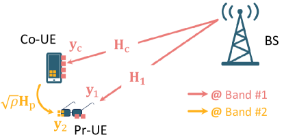
Figure 1: A UE-CoMIMO System.

In recent years, the proliferation of personal devices such as smartphones, wearable devices, and portable chargers within personal area networks has created opportunities for deeper physical layer collaboration, effectively increasing the number of available antenna elements. This concept, known as end-user-centric collaborative MIMO (UE-CoMIMO) [7], was proposed in 3GPP [8]. It enables multiple devices to collaboratively process their received signals, thereby augmenting the number of antennas and enhancing the number of spatial streams.

As illustrated in Fig. 1, in a UE-CoMIMO setup, the base station (BS) simultaneously transmits data to both the primary UE and a nearby collaborative UE using a low-frequency band. The collaborative UE then amplifies and forwards its received signal to the primary UE via a high-frequency band. The primary UE can either utilize additional high-frequency antennas or share antennas across both low- and high-frequency bands. This flexibility is further enhanced by the smaller size of high-frequency antennas, making them easier to integrate into the compact spaces of terminal devices. This configuration effectively increases the number of antennas available to the primary UE. For example, extended reality glasses equipped with two antennas could collaborate with a smartphone that has four antennas, resulting in a combined six-antenna system capable of supporting higher-order MIMO ranks.

While the concept of frequency-translation amplify-and-forward (AF) relays has been previously proposed to assist antenna-limited UEs [9, 10], these approaches primarily leverage frequency division multiplexing to enhance spatial diversity rather than focusing on spatial multiplexing. Although UE-CoMIMO [7] has demonstrated improvements in spatial diversity and multiplexing through system-level simulations, it lacks a comprehensive mathematical problem formulation and dedicated optimization algorithms. To address this gap, [11] recently formulated the rate maximization problem for the UE-CoMIMO system and derived optimization algorithms for the relay amplifying matrix, with a focus primarily on the uplink system. In this paper, we shift our focus to the downlink system and evaluate the UE-CoMIMO system from various practical perspectives that are more aligned with the use cases of personal area networks. These perspectives enable us to implement the UE-CoMIMO system in a manner that validates the concepts derived from this study. Our main contributions are as follows:

• Theoretical Performance Analysis of the UE-CoMIMO System: We provide a theoretical framework for analyzing the spectral efficiency (SE) of the UE-CoMIMO system, focusing on the singular values of its reformulated channel matrix. This matrix is constructed by incorporating the relay link’s channel matrix as an additional row to the original channel matrix from the BS. Our analysis shows that incorporating the relay link consistently enhances the singular values, thereby improving system performance even without phase optimization. This is in contrast to reconfigurable intelligent surfaces (RIS), where performance gains rely heavily on precise phase optimization [12, 13, 14, 15].

• Optimization Algorithms for Relay Phase Adjustment: Prior works [10, 11] assume fully connected relay structures between low- and high-frequency antennas, allowing both amplitude and phase adjustments, which may be impractical for terminal devices. In this paper, we explore simpler relay structures, such as parallel phase-adjustable links between low- and high-frequency antennas (multiplexing structure) or a single link through a phase combiner/splitter between low- and high-frequency antennas (diversity structure). We develop optimization algorithms for phase adjustment in these structures that efficiently achieve near-optimal settings without requiring full CSI of the relay link. This approach results in a straightforward protocol and a practical, implementable algorithm.

• Simulations and Experimental Validation: The performance of the UE-CoMIMO system is sensitive to the relative positioning of collaborating devices. We conducted ray-tracing simulations in both indoor and outdoor scenarios, demonstrating that different relay structures are required for different use cases. These simulations provided key insights. Additionally, we implemented the UE-CoMIMO system in real-world settings, validating the results and demonstrating its practical viability.

The remainder of this paper is organized as follows: Section II presents the system model for the UE-CoMIMO system. Section III analyzes the SE of the system and develops algorithms for optimizing the relay phases. Section IV includes extensive simulations, such as ray-tracing, to explore the properties of optimal phases and their performance in various scenarios. Section V discusses the system implementation and evaluates its performance through over-the-air testing. Finally, Section VI concludes the paper.

II System Model

As shown in Fig. 1, we consider a MIMO system comprising a BS and primary UE (Pr-UE). The transmission from the BS to Pr-UE occurs through the $f_{\rm L}$ band. The transmitted signal, denoted as ${\bf x}$, passes through the wireless channel and is received by both Pr-UE and the collaborative UE (Co-UE). The received signals at Pr-UE and Co-UE can be expressed as, respectively,

$${\bf y}_{1} ={\bf H}_{1}{\bf x}+{\bf z}_{1},$$ (1a)

$${\bf y}_{\rm c} ={\bf H}_{\rm c}{\bf x}+{\bf z}_{\rm c}.$$ (1b)

Here, ${\bf H}_{1}\in{\mathbb{C}}^{N_{1}\times M}$ is the channel matrix between the BS and Pr-UE (referred to as the direct link) with $M$ transmit antennas and $N_{1}$ receive antennas. ${\bf H}_{\rm c}\in{\mathbb{C}}^{N_{\rm c}\times M}$ denotes the channel between the BS and Co-UE, referred to as the first-hop channel, with $N_{\rm c}$ representing the number of receive antennas at Co-UE. ${\bf z}_{1}\in{\mathbb{C}}^{N_{1}\times 1}$ and ${\bf z}_{\rm c}\in{\mathbb{C}}^{N_{\rm c}\times 1}$ are complex Gaussian noise vectors added at Pr-UE and Co-UE, respectively.

The Co-UE employs a frequency-translation AF repeater to transfer its received signal ${\bf y}_{\rm c}$ to another frequency band denoted as $f_{\rm H}$. It then contributes to the received signals at Pr-UE as

$${\bf y}_{2}=\sqrt{\rho}\,{\bf H}_{\rm p}{\bf y}_{\rm c}+{\bf z}_{2}\approx\sqrt{\rho}\,{\bf H}_{\rm p}{\bf H}_{\rm c}{\bf x}+{\bf z}_{2},$$ (2)

where ${{\bf H}_{\rm p}\in{\mathbb{C}}^{N_{2}\times N_{\rm c}}}$ denotes the relay channel between Co-UE and Pr-UE, and $\rho$ represents the power gain from the low-noise amplifier (LNA) for the second-hop link. The vector ${\bf z}_{\rm 2}$ represents the complex Gaussian noise vector added at Pr-UE. Unlike a conventional repeater, this setup uses LNAs in Co-UE, which only amplify the signal by a few dBs as opposed to the conventional repeater with an amplification gain of up to 90-100 dB. The Co-UE does not introduce significant noise. Consequently, we ignore the noise contribution of ${\bf z}_{\rm c}$ and obtain an approximation in (2).

For ease of exposition, we define ${\bf H}_{2}=\sqrt{\rho}\,{\bf H}_{\rm p}{\bf H}_{\rm c}\in{\mathbb{C}}^{N_{2}\times M}$, and

$${\bf H}=\begin{bmatrix}{\bf H}_{1}\\ {\bf H}_{2}\end{bmatrix},~{}{\bf y}=\begin{bmatrix}{\bf y}_{1}\\ {\bf y}_{2}\end{bmatrix},~{}{\bf z}=\begin{bmatrix}{\bf z}_{1}\\ {\bf z}_{2}\end{bmatrix}.$$ (3)

Note that ${\bf H}\in{\mathbb{C}}^{(N_{1}+N_{2})\times M}$ and ${\bf y},{\bf z}\in{\mathbb{C}}^{(N_{1}+N_{2})\times 1}$. We then rewrite the end-to-end input-output relation of this system in a more compact manner as

$${\bf y}={\bf H}{\bf x}+{\bf z}.$$ (4)

For ease of the following analysis and without loss of generality, we assume that the noise vector ${\bf z}$ has been pre-whitened, and thus it represents the complex standard Gaussian noise vector.

Note that UE-CoMIMO schemes differ from direct communication using dual spectrum because the BS does not utilize dual spectrum simultaneously [7]. Typically, Co-UE is a nearby device close to Pr-UE with low transmission power, causing minimal network interference. Therefore, UE-CoMIMO schemes are not considered to use dual spectrum. From the network’s perspective, the BS communicates with an aggregated user, formed by multiple devices in the $f_{\rm L}$ band, while still being able to reuse the $f_{\rm H}$ band to serve other UEs. The work in [7] has demonstrated that enabling UE-CoMIMO provides additional gains over conventional carrier aggregation schemes, which involve direct transmission from UE to BS in both $f_{\rm L}$ and $f_{\rm H}$ bands, as shown through system-level evaluations.

III Performance Analysis and Customize ${\bf H}_{2}$

The SE of the UE-CoMIMO system highly depends on the singular value of ${\bf H}$, which is formulated by appending ${\bf H}_{2}$ in row to ${\bf H}_{1}$. We express the singular value decomposition (SVD) of ${\bf H}_{1}$ as

$${\bf H}_{1}={\bf U}_{{\rm H}_{1}}{\boldsymbol{\Sigma}}_{{\rm H}_{1}}{\bf V}_{{\rm H}_{1}}^{\rm H},$$ (5)

where ${\bf U}_{{\rm H}_{1}}\in{\mathbb{C}}^{N_{1}\times N_{1}}$ and ${\bf V}_{{\rm H}_{1}}\in{\mathbb{C}}^{M\times M}$ are unitary matrices, ${\boldsymbol{\Sigma}}_{{\rm H}_{1}}\in{\mathbb{R}}^{N_{1}\times M}$ is zero except on the main diagonal, which contains non-negative entries in decreasing order. The column of ${\bf U}_{{\rm H}_{1}}$ and ${\bf V}_{{\rm H}_{1}}$ are the left singular vectors and the right singular vector of ${\bf H}_{1}$, respectively; the diagonal entries of ${\boldsymbol{\Sigma}}_{{\rm H}_{1}}$ are the singular values of ${\bf H}_{1}$, arranged as follows:

$$\sigma_{1}({\bf H}_{1})\geq\cdots\geq\sigma_{M-1}({\bf H}_{1})\geq\sigma_{M}({\bf H}_{1})\geq 0.$$ (6)

Similarly, we can express the SVD of ${\bf H}$ as

$${\bf H}={\bf U}_{{\rm H}}{\boldsymbol{\Sigma}}_{{\rm H}}{\bf V}_{{\rm H}}^{\rm H},$$ (7)

where ${\bf U}_{{\rm H}}\in{\mathbb{C}}^{(N_{1}+N_{2})\times(N_{1}+N_{2})}$, ${\bf V}_{{\rm H}}\in{\mathbb{C}}^{M\times M}$ are unitary matrices, and ${\boldsymbol{\Sigma}}_{{\rm H}}\in{\mathbb{R}}^{(N_{1}+N_{2})\times M}$ with the real numbers

$$\sigma_{1}({\bf H})\geq\cdots\geq\sigma_{M-1}({\bf H})\geq\sigma_{M}({\bf H})\geq 0$$ (8)

on the diagonal.

This section explains how the singular values of ${\bf H}$ can be modified from those of ${\bf H}_{1}$ using ${\bf H}_{2}$. We start by demonstrating that the singular values of ${\bf H}$ can be represented as a rank-$N_{2}$ modification of the singular values of ${\bf H}_{1}$ in the following subsection. Then, we explicitly express the singular value update in terms of ${\bf H}_{1}$ and ${\bf H}_{2}$. Finally, we illustrate how to customize the channel ${\bf H}_{2}$ by introducing phase shifters and develop an efficient algorithm for this purpose.

III-A Rank-$N_{2}$ Modification

First, consider the case $N_{1}\geq M$. We define the matrices as follows:

$${\bf U}_{{\rm H}_{1}}=\begin{bmatrix}{\bf U}_{{{\rm H}_{1}},1}~{}{\bf U}_{{{\rm H}_{1}},2}\end{bmatrix}~{}\mbox{and}~{}{\boldsymbol{\Sigma}}_{{\rm H}_{1}}=\begin{bmatrix}{\bf D}_{{\rm H}_{1}}\\ {\bf 0}\end{bmatrix},$$ (9)

where ${\bf U}_{{{\rm H}_{1}},1}\in{\mathbb{C}}^{N_{1}\times M}$, ${\bf U}_{{{\rm H}_{1}},2}\in{\mathbb{C}}^{N_{1}\times(N_{1}-M)}$, and ${\bf D}_{{\rm H}_{1}}\in{\mathbb{R}}^{M\times M}$. Note that ${\bf D}_{{\rm H}_{1}}$ is a diagonal matrix containing the nonzero singular values of ${\bf H}_{1}$ on its diagonal. By substituting (9) into ${\bf H}$ defined in (3), ${\bf H}$ can be expressed as:

$${\bf H}=\begin{bmatrix}{\bf U}_{{\rm H}_{1},1}&{\bf 0}&{\bf U}_{{\rm H}_{1},2}\\ {\bf 0}&{\bf I}_{N_{2}}&{\bf 0}\end{bmatrix}\begin{bmatrix}{\bf D}_{{\rm H}_{1}}\\ {\bf H}^{\prime}_{2}\\ {\bf 0}\end{bmatrix}{\bf V}_{1}^{\rm H},$$ (10)

where ${\bf H}^{\prime}_{2}={\bf H}_{2}{\bf V}_{1}\in{\mathbb{C}}^{N_{2}\times M}$. We define ${\bf A}$ as

$${\bf A}=\begin{bmatrix}{\bf D}_{{\rm H}_{1}}\\ {\bf H}^{\prime}_{2}\end{bmatrix}\in{\mathbb{C}}^{(M+N_{2})\times M}.$$ (11)

Since the matrices on both sides of (10) are unitary matrices, computing the singular values of ${\bf H}$ is equivalent to performing the SVD of ${\bf A}$.

Specifically, we express the SVD of ${\bf A}$ as

$${\bf A}=\begin{bmatrix}{\bf U}_{{\rm A},1}~{}{\bf U}_{{\rm A},2}\end{bmatrix}\begin{bmatrix}{\bf D}_{\rm A}\\ {\bf 0}\end{bmatrix}{\bf V}_{\rm A}^{\rm H},$$ (12)

with ${\bf U}_{{\rm A},1}\in{\mathbb{C}}^{(M+N_{2})\times M}$, ${\bf U}_{{\rm A},2}\in{\mathbb{C}}^{(M+N_{2})\times N_{2}}$, ${\bf D}_{\rm A}\in{\mathbb{R}}^{M\times M}$, and ${\bf V}_{\rm A}\in{\mathbb{C}}^{M\times M}$. By combining (11) and (12), we obtain

$${\bf A}^{\rm H}{\bf A}={\bf D}_{{\rm H}_{1}}^{2}+({\bf H}^{\prime}_{2})^{{\rm H}}{\bf H}^{\prime}_{2}={\bf V}_{{\rm A}}{\bf D}_{\rm A}^{2}{\bf V}_{{\rm A}}^{\rm H},$$ (13)

which is the rank-$N_{2}$ modification of ${\bf D}_{{\rm H}_{1}}^{2}$. Similarly, in the case where $N_{1}<M$, we can apply the same reasoning.

III-B Singular Value Update

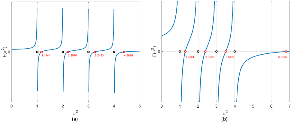
Figure 2: Graph of the secular equation with $\sigma_{i}^{2}({\bf H}_{1})=(1,2,3,4)$ for (a) $\|{\bf h}^{\prime}\|_{2}^{2}=1$ and (b) $\|{\bf h}^{\prime}\|_{2}^{2}=4$.

The task of updating the SVD involves matrix perturbation processes. The following lemma characterizes the singular values of ${\bf H}$.

Lemma 1

[16, Corollary 4.3.3] The singular values of ${\bf H}$ satisfy

$$\sigma_{m}({\bf H})\geq\sigma_{m}({\bf H}_{1}).$$ (14)

With Lemma 1, it becomes evident that the additional channel from ${\bf y}_{2}$ definitively increases the effective channel gain (or the singular values of ${\bf H}$) of the system. To further elucidate the impact on the singular values of ${\bf H}$ relative to ${\bf H}_{1}$, we initially consider a special case where $N_{2}=1$. The derived results can be extended to general values of $N_{2}$ by iterating the obtained results. For $N_{2}=1$, we simply denote ${\bf H}_{2}\in{\mathbb{C}}^{1\times M}$ by ${\bf h}_{2}$ and ${\bf H}^{\prime}_{2}$ by ${\bf h}^{\prime}=[h^{\prime}_{1},\ldots,h^{\prime}_{M}]$. We then express (11) as:

$${\bf A}=\bNiceMatrix[margin]\Block[fill=red!10,rounded-corners]{3-3}{}\sigma_{1}({\bf H}_{1})&{\bf 0}\\ \ddots\\ {\bf 0}\sigma_{M}({\bf H}_{1})\\ \Block[fill=blue!10,rounded-corners]{*-*}{}h^{\prime}_{1}\cdots h^{\prime}_{M}.$$ (15)

Subsequently, (13) is formulated as:

$${\bf A}^{\rm H}{\bf A}={\bf D}_{{\rm H}_{1}}^{2}+({\bf h}^{\prime})^{{\rm H}}{\bf h}^{\prime},$$ (16)

representing a rank-one modification of ${\bf D}_{{\rm H}_{1}}^{2}$.

Note that ${\bf h}^{\prime}={\bf h}_{2}{\bf V}_{{\rm H}_{1}}$ indicates that vector ${\bf h}_{2}$ projects onto ${{\bf V}_{{\rm H}_{1}}=[{\bf v}_{{\rm H}_{1},1},\ldots,{\bf v}_{{\rm H}_{1},M}]}$, with each vector ${\bf v}_{{\rm H}_{1},m}$ corresponding to the right singular vectors of ${\bf H}_{1}$ in decreasing order. The value of each element, $h^{\prime}_{i}$, thus reflects the similarity between ${\bf h}_{2}$ and each ${\bf v}_{{\rm H}_{1},i}$. For the rank-one modification of ${\bf D}_{{\rm H}_{1}}^{2}$, we consider the following lemma:

Lemma 2

[17, Theorem 8.5.3] The singular values $\{\sigma_{i}({\bf H})\}$ satisfy the interlacing property

$$\sigma_{1}({\bf H}_{1})+\|{\bf h}^{\prime}\|_{2}\geq\sigma_{1}({\bf H})\geq\sigma_{1}({\bf H}_{1})>\cdots\\ \geq\sigma_{M-1}({\bf H}_{1})\geq\sigma_{M}({\bf H})\geq\sigma_{M}({\bf H}_{1})\geq 0,$$ (17)

and the secular equation

$$F(\sigma^{2})=1+\sum_{i=1}^{M}\frac{|h^{\prime}_{i}|^{2}}{\sigma_{i}^{2}({\bf H}_{1})-\sigma^{2}}=0.$$ (18)

Some insights can be observed from this lemma:

O1: First, the secular equation indicates that $\sigma_{i}({\bf H})$ should be larger than $\sigma_{i}({\bf H}_{1})$ and follows the interlacing property (17). Fig. 2(a) shows an example of the secular equation for $M=4$, $\sigma_{i}^{2}({\bf H}_{1})=(1,2,3,4)$ and ${\bf h}^{\prime}=(1/2,1/2,1/2,1/2)$. The singular values of ${\bf H}_{1}$ are marked in black “$\circ$”, while those of ${\bf H}$ are marked in red “${\color[rgb]{1,0,0}\circ}$”. Specifically, $\sigma_{i}^{2}({\bf H})$ satisfies:

$$1+\frac{1}{4}\left(\frac{1}{4-\sigma^{2}}+\frac{1}{3-\sigma^{2}}+\frac{1}{2-\sigma^{2}}+\frac{1}{1-\sigma^{2}}\right)=0.$$ (19)

The secular function $F(\sigma^{2})$ is monotone in between its poles. Thus, $F(\sigma^{2})$ has precisely 4 roots, one in each of the intervals

$$(1,2),\,(1,2),\,(3,4),\,(4,\infty).$$ (20)

O2: Second, all the singular values undergo specific modifications from their corresponding $\sigma_{i}^{2}({\bf H}_{1})$, with the largest singular value $\sigma_{\max}^{2}({\bf H})$ experiencing the most substantial change and the smallest singular value $\sigma_{\min}^{2}({\bf H})$ the least. To observe this, we let $\Delta_{i}=\sum_{m\neq i}{|h^{\prime}_{m}|^{2}}/{(\sigma_{m}^{2}({\bf H}_{1})-\sigma^{2})}$. Applying (18), we derive

$$\sigma_{i}^{2}({\bf H})=\sigma_{i}^{2}({\bf H}_{1})+\frac{|h^{\prime}_{i}|^{2}}{1+\Delta_{i}}.$$ (21)

Note that $\Delta_{i}$ has a lower bound of $-1$ but no upper bound. For the largest singular value, $\Delta_{i}$ assumes the most negative value; conversely, for the smallest singular value, it assumes the largest positive value, leading to our second observation.

O3: Third, if $h^{\prime}_{i}$ is small, then the change in $\sigma_{i}^{2}({\bf H})$ from $\sigma_{i}^{2}({\bf H}_{1})$ is also minimal. Conversely, if $h^{\prime}_{i}$ dominates, the change in $\sigma_{i}^{2}({\bf H})$ also dominates. This observation is directly derived from (21). For the special case where $h^{\prime}_{i}=0$, the singular value $\sigma_{i}^{2}({\bf H})$ is unchanged.

O4: Fourth, if ${\bf h}^{\prime}$ is uniformly spread across elements and $\|{\bf h}^{\prime}\|_{2}$ sufficiently large, it will predominantly contribute to the largest singular value. This observation can be derived from the interlacing property (17). Fig. 2(b) demonstrates this observation.

With these observations, we can conclude that by properly designing ${\bf h}^{\prime}$ (or equivalently ${\bf h}_{2}$), we can improve the system solely in the direction of increase. This capability of UE-CoMIMO brings to mind the recently popular technology of RIS. Like UE-CoMIMO, the additional path contributed by RIS can be viewed as a rank modification of ${\bf H}_{1}$, expressed as

$${\bf H}={\bf H}_{1}+{\bf a}{\bf h}^{\prime}.$$ (22)

However, unlike UE-CoMIMO, RIS does not necessarily enhance the singular values of the new channel ${\bf H}$, as described in (14) in Lemma 1. As shown in [18], the singular values $\sigma_{m}({\bf H})$ of (22) may be lower bounded by $\sigma_{m}({\bf H}_{1})-\|{\bf a}\|_{2}\|{\bf h}^{\prime}\|_{2}$. This indicates that if not properly designed, RIS can potentially reduce the effective channel gain.

III-C Customize ${\bf H}_{2}$

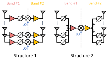
Figure 3: Illustration of two structures employing phasors at Co-UE.

In the previous subsection, we have demonstrated that the additional channel ${\bf H}_{2}$ appending in row to ${\bf H}_{1}$ definitively increases the SE of the system. In this subsection, we aim to customize the channel ${\bf H}_{2}$ by introducing phase shifters (PSs). We consider two structures for this purpose.

In Structure 1, as shown in Fig. 3, each frequency-translation element consists of a receive antenna, a low-frequency LNA, a low-frequency PS, a high-frequency LNA, and a transmit antenna. Recall that we have $N_{\rm c}$ antennas at Co-UE, which implies there are $N_{\rm c}$ frequency-translation elements. For ease of expression, we define the transmission coefficients of the PSs as ${\boldsymbol{\Phi}}_{\rm s1}={\sf diag}({\boldsymbol{\phi}}_{\rm s1})$ with ${\boldsymbol{\phi}}_{\rm s1}=[e^{j\theta_{1}},\ldots,e^{j\theta_{N_{\rm c}}}]^{\rm T}$. Then, ${\bf H}_{2}$ in Structure 1 can be expressed as:

$${\bf H}_{2}=\sqrt{\rho}\,{\bf H}_{\rm p}{\boldsymbol{\Phi}}_{\rm s1}{\bf H}_{\rm c}.$$ (23)

We can customize the channel ${\bf H}_{2}$ by adjusting $\theta_{n}$ within $(0,2\pi]$ for $n=1,\ldots,N_{\rm c}$. That is, the elements of ${\boldsymbol{\phi}}_{\rm s1}$ are assume to satisfy $|\phi_{{\rm s1},n}|=1$ for $n=1,\ldots,N_{\rm c}$, which is simply denoted by $|{\boldsymbol{\phi}}_{\rm s1}|={\bf 1}$.

In Structure 2, as shown in Fig. 3, each frequency-translation element includes $N_{\rm c}$ receive antennas, $N_{\rm c}$ low-frequency PSs, a power combiner, a low-frequency LNA, a mixer, a high-frequency LNA, a power splitter, $N_{\rm c}$ high-frequency PSs, and $N_{\rm c}$ transmit antennas. We define the coefficients of the PS for the power combiner and the coefficients of the PS for the power splitter as:

$${\boldsymbol{\phi}}_{\rm r} =[e^{j\theta_{{\rm r},1}},\ldots,e^{j\theta_{{\rm r},N_{\rm c}}}]^{\rm T},$$ (24a)

$${\boldsymbol{\phi}}_{\rm t} =[e^{j\theta_{{\rm t},1}},\ldots,e^{j\theta_{{\rm t},N_{\rm c}}}]^{\rm T}.$$ (24b)

Then, ${\bf H}_{2}$ in Structure 2 can be expressed as:

$${\bf H}_{2}=\sqrt{\rho}\,{\bf H}_{\rm p}{\boldsymbol{\phi}}_{\rm t}{\boldsymbol{\phi}}_{\rm r}^{\rm H}{\bf H}_{\rm c}=\sqrt{\rho}\,{\bf H}_{\rm p}{\boldsymbol{\Phi}}_{\rm s2}{\bf H}_{\rm c},$$ (25)

where ${\boldsymbol{\Phi}}_{\rm s2}={\boldsymbol{\phi}}_{\rm t}{\boldsymbol{\phi}}_{\rm r}^{\rm H}$. Also, the channel ${\bf H}_{2}$ can be customized by adjusting $(\theta_{{\rm r},n},\theta_{{\rm t},n})$ for $n=1,\ldots,N_{\rm c}$, and we assume $|{\boldsymbol{\phi}}_{\rm t}|={\bf 1}$ and $|{\boldsymbol{\phi}}_{\rm r}|={\bf 1}$.

TABLE I: Power Consumption of RF Elements.

Element	Product #	Power
Low Frequency LNA	ZX60-3800LN-S+	425 mW
Low Frequency PS	MAP-010144	0.15 mW
High Frequency LNA	ZX60-05113LN+	180 mW
High Frequency PS	TGP2105-SM	0.15 mW
Mixer	ZX05-83-S+	$\sim$ 0 mW

For ease of expression, we use ${\boldsymbol{\Phi}}_{\rm s}$ to denote either ${\boldsymbol{\Phi}}_{\rm s1}$ or ${\boldsymbol{\Phi}}_{\rm s2}$. The channel ${\bf H}_{2}$ in both structures 1 and 2 is formed by the product of three matrices $({\bf H}_{\rm p},{\boldsymbol{\Phi}}_{\rm s},{\bf H}_{\rm c})$. The rank of ${\bf H}_{2}$ is determined by $\min\{{\sf rank}({\bf H}_{\rm p}),{\sf rank}({\boldsymbol{\Phi}}_{\rm s}),{\sf rank}({\bf H}_{\rm c})\}$. Clearly, ${\bf H}_{2}$ in Structure 2 is rank 1, which eventually leads to rank-1 modification of ${\bf H}_{1}$. According to the observations from Lemma 2 (i.e., O2 and O3), Structure 2 (or rank-1 modification) can only slightly modify the singular value of ${\bf H}_{1}$, with the most substantial change to the largest singular value of ${\bf H}_{1}$ or one singular value. Therefore, the modification offered by Structure 2 is not comprehensive. In contrast, Structure 1 can perform a rank-$N_{2}$ modification of ${\bf H}_{1}$, resulting in a more sophisticated update on the singular values of ${\bf H}_{1}$. However, Structure 1 needs multiple mixers, resulting in high cost than Structure 2.

In Section V, we implemented both Structure 1 and Structure 2. Table I displays the power consumption for the RF elements involved in each structure. The power consumptions for Structures 1 and 2 are calculated as follows

$$P_{{\rm s1}} =N_{\rm c}\times(425+0.15+180),$$ (26a)

$$P_{{\rm s2}} =N_{\rm c}\times 0.15+425+180+N_{\rm c}\times 0.15.$$ (26b)

Given that the power consumption from the PSs is minor compared to that from the LNAs, the power consumption of Structure 1 is almost $N_{\rm c}$ times higher than that of Structure 2. For example, with $N_{\rm c}=4$, the calculated power consumption amounts to $P_{{\rm s1}}=2420.6$ mW and $P_{{\rm s2}}=606.2$ mW.

To specify a method for adjusting ${\boldsymbol{\Phi}}_{\rm s}$, consider the SE of the UE-CoMIMO system, which is given by:

$$C =\log\det{\left({\bf I}_{N_{1}+N_{2}}+{\bf H}{\bf H}^{\rm H}\right)},$$ (27)

$$=\log\det{\left({\bf I}_{M}+{\bf D}_{{\rm H}_{1}}^{2}+({\bf H}^{\prime}_{2})^{{\rm H}}{\bf H}^{\prime}_{2}\right)},$$

$$=\underbrace{\log\det{\left({\bf I}_{M}+{\bf D}_{{\rm H}_{1}}^{2}\right)}}_{\text{SE of original Pr-UE}}$$

$$\quad+\underbrace{\log\det{\left({\bf I}_{N_{2}}+{\bf H}^{\prime}_{2}({\bf I}_{M}+{\bf D}_{{\rm H}_{1}}^{2})^{-1}({\bf H}^{\prime}_{2})^{{\rm H}}\right)}}_{\text{Gain from Co-UE}},$$ (28)

where the second equality follows from footnote 1 and (13), and in the third equality, we utilize the fact that $\det({\bf A}{\bf B})=\det({\bf A})\det({\bf B})$ and $\det({\bf I}+{\bf A}{\bf B})=\det({\bf I}+{\bf B}{\bf A})$. The second term of (28) represents the contribution from the additional channel ${\bf y}_{2}$ of the UE-CoMIMO system, which heavily depends on ${\bf H}^{\prime}_{2}$. Recall from the previous subsection that the modification of singular values also heavily depends on ${\bf H}^{\prime}_{2}$.

We initially consider maximizing the SE with Structure 2. Recall that ${\bf H}^{\prime}_{2}={\bf H}_{2}{\bf V}_{{\rm H}_{1}}$. Applying (25), we have

$${\bf H}^{\prime}_{2}={\bf H}_{2}{\bf V}_{{\rm H}_{1}}=\sqrt{\rho}\,{\bf H}_{\rm p}{\boldsymbol{\phi}}_{\rm t}{\boldsymbol{\phi}}_{\rm r}^{\rm H}{\bf H}_{\rm c}{\bf V}_{{\rm H}_{1}}.$$ (29)

The Gram matrix $({\bf H}^{\prime}_{2})^{\rm H}{\bf H}^{\prime}_{2}$ is expressed as

$$({\bf H}^{\prime}_{2})^{\rm H}{\bf H}^{\prime}_{2}=\rho\,{\bf V}_{{\rm H}_{1}}^{\rm H}{\bf H}_{\rm c}^{\rm H}{\boldsymbol{\phi}}_{\rm r}{\boldsymbol{\phi}}_{\rm t}^{\rm H}{\bf H}_{\rm p}^{\rm H}{\bf H}_{\rm p}{\boldsymbol{\phi}}_{\rm t}{\boldsymbol{\phi}}_{\rm r}^{\rm H}{\bf H}_{\rm c}{\bf V}_{{\rm H}_{1}}.$$ (30)

We define $\eta={\boldsymbol{\phi}}_{\rm t}^{\rm H}{\bf H}_{\rm p}^{\rm H}{\bf H}_{\rm p}{\boldsymbol{\phi}}_{\rm t}$ and ${\boldsymbol{\omega}}={\bf V}_{{\rm H}_{1}}^{\rm H}{\bf H}_{\rm c}^{\rm H}{\boldsymbol{\phi}}_{\rm r}$. Substituting (30) along with these definitions into (28), we obtain

$$C=\sum_{m=1}^{M}\log(1+\sigma_{m}^{2}({\bf H}_{1}))+\log{\left(1+\rho\,\eta\,{\boldsymbol{\omega}}^{\rm H}({\bf I}+{\bf D}_{{\rm H}_{1}}^{2})^{-1}{\boldsymbol{\omega}}\right)}.$$ (31)

Note that $\eta$ and ${\boldsymbol{\omega}}$ are function of ${\boldsymbol{\phi}}_{\rm t}$ and ${\boldsymbol{\phi}}_{\rm r}$. Maximizing the SE is equivalent to maximizing $\rho\,\eta\,{\boldsymbol{\omega}}^{\rm H}({\bf I}+{\bf D}_{{\rm H}_{1}}^{2})^{-1}{\boldsymbol{\omega}}=\rho\,\eta\,{\boldsymbol{\phi}}_{\rm r}^{\rm H}{\bf H}_{\rm c}{\bf V}_{{\rm H}_{1}}({\bf I}+{\bf D}_{{\rm H}_{1}}^{2})^{-1}{\bf V}_{{\rm H}_{1}}^{\rm H}{\bf H}_{\rm c}^{\rm H}{\boldsymbol{\phi}}_{\rm r}$, which can be expressed as

$$\max_{{\boldsymbol{\phi}}_{\rm t},\,{\boldsymbol{\phi}}_{\rm r}} ~{}~{}\rho\,\eta\,{\boldsymbol{\phi}}_{\rm r}^{\rm H}{\bf H}_{\rm c}({\bf I}_{M}+{\bf H}_{1}^{\rm H}{\bf H}_{1})^{-1}{\bf H}_{\rm c}^{\rm H}{\boldsymbol{\phi}}_{\rm r},$$

$${\rm s.t.} ~{}~{}|{\boldsymbol{\phi}}_{\rm t}|={\bf 1},~{}|{\boldsymbol{\phi}}_{\rm r}|={\bf 1}.$$ (P2)

Interestingly, the optimality of ${\boldsymbol{\phi}}_{\rm t}$ can be achieved only through maximizing $\eta$. Consequently, the optimality of ${\boldsymbol{\phi}}_{\rm t}$ and ${\boldsymbol{\phi}}_{\rm r}$ can be determined separately. This characteristic significantly simplifies the complexity involved in determining their optimal configurations. Define

$$\widetilde{{\bf H}}_{\rm c}={\bf H}_{\rm c}\left({\bf I}_{M}+{\bf H}_{1}^{\rm H}{\bf H}_{1}\right)^{-1/2},$$ (32)

${\boldsymbol{\Phi}}_{\rm t}={\boldsymbol{\phi}}_{\rm t}{\boldsymbol{\phi}}_{\rm t}^{\rm H}$, and ${\boldsymbol{\Phi}}_{\rm r}={\boldsymbol{\phi}}_{\rm r}{\boldsymbol{\phi}}_{\rm r}^{\rm H}$. Then, the optimality of ${\boldsymbol{\phi}}_{\rm t}$ and ${\boldsymbol{\phi}}_{\rm r}$ can be formulated into the following two problems:

$$\max_{{\boldsymbol{\Phi}}_{\rm t}} ~{}~{}{\sf tr}({\bf H}_{\rm p}^{\rm H}{\bf H}_{\rm p}{\boldsymbol{\Phi}}_{\rm t}),$$

$${\rm s.t.} ~{}~{}[{\boldsymbol{\Phi}}_{\rm t}]_{n,n}=1,~{}n=1,\ldots,N_{\rm c},~{}{\boldsymbol{\Phi}}_{\rm t}\succeq{\bf 0},$$ (P2-1)

and

$$\max_{{\boldsymbol{\Phi}}_{\rm r}} ~{}~{}{\sf tr}(\widetilde{{\bf H}}_{\rm c}\widetilde{{\bf H}}_{\rm c}^{\rm H}{\boldsymbol{\Phi}}_{\rm r}),$$

$${\rm s.t.} ~{}~{}[{\boldsymbol{\Phi}}_{\rm r}]_{n,n}=1,~{}n=1,\ldots,N_{\rm c},~{}{\boldsymbol{\Phi}}_{\rm r}\succeq{\bf 0}.$$ (P2-2)

Note that these problems also need to satisfy the rank constraints: ${\sf rank}({\boldsymbol{\Phi}}_{\rm t})=1$ and ${\sf rank}({\boldsymbol{\Phi}}_{\rm r})=1$, consistent with the definitions of ${\boldsymbol{\Phi}}_{\rm t}$ and ${\boldsymbol{\Phi}}_{\rm r}$. Together with the above discussions, we present the following theorem to establish the optimality of Structure 2.

Theorem 1

The optimality of ${\boldsymbol{\phi}}_{\rm t}$ and ${\boldsymbol{\phi}}_{\rm r}$ can be determined separately. In a special case with ${\sf rank}({\bf H}_{\rm p})=1$ and ${\sf rank}(\widetilde{{\bf H}}_{\rm c})=1$, the maximal SE can be achieved by setting

$${\boldsymbol{\phi}}_{\rm t}=e^{-j\arg({\bf v}_{{\rm H}_{\rm p},1})},~{}~{}{\boldsymbol{\phi}}_{\rm r}=e^{-j\arg({\bf u}_{\widetilde{\rm H}_{\rm c},1})},$$ (33)

where ${\bf v}_{{\rm H}_{\rm p},1}$ is the first right singular vector of ${\bf H}_{\rm p}$, and ${\bf u}_{\widetilde{\rm H}_{\rm c},1}$ is the first left singular vector of $\widetilde{{\bf H}}_{\rm c}$.

Later in Section IV-C, we demonstrate that the case where ${{\sf rank}({\bf H}_{\rm p})=1}$ frequently occurs in practical applications as the distance between Co-UE and Pr-UE increases. However, the two optimization problems in (P2-1) and (P2-2) are generally non-convex and challenging to solve. To find a solution, we may employ semidefinite relaxation (SDR) to relax the rank-one constraint. Nonetheless, the relaxed problem may not yield a rank-one solution, indicating that additional steps are necessary to derive a rank-one solution from the higher-rank solution obtained. Further details on this process can be found in [19] and are thus omitted here.

Next, we consider maximizing the SE for Structure 1. Applying (23), we have

$${\bf H}^{\prime}_{2}={\bf H}_{2}{\bf V}_{{\rm H}_{1}}=\sqrt{\rho}\,{\bf H}_{\rm p}{\boldsymbol{\Phi}}_{\rm s1}{\bf H}_{\rm c}{\bf V}_{{\rm H}_{1}}.$$ (34)

Moreover, we write $\widetilde{{\bf H}}_{\rm c}\widetilde{{\bf H}}_{\rm c}^{\rm H}$ as

$$\widetilde{{\bf H}}_{\rm c}\widetilde{{\bf H}}_{\rm c}^{\rm H}=\sum_{m=1}^{M}\sigma_{{\widetilde{\rm H}_{\rm c}},m}^{2}{\bf u}_{{\widetilde{\rm H}_{\rm c}},m}{\bf u}_{{\widetilde{\rm H}_{\rm c}},m}^{\rm H},$$ (35)

Thus, the Gram matrix ${\bf H}^{\prime}_{2}({\bf I}_{M}+{\bf D}_{{\rm H}_{1}}^{2})^{-1}({\bf H}^{\prime}_{2})^{{\rm H}}$ is expressed as

$${\bf H}^{\prime}_{2}({\bf I}_{M}+{\bf D}_{{\rm H}_{1}}^{2})^{-1}({\bf H}^{\prime}_{2})^{{\rm H}}$$

$$=\rho\,{\bf H}_{\rm p}{\boldsymbol{\Phi}}_{\rm s1}{\bf H}_{\rm c}{\bf V}_{{\rm H}_{1}}({\bf I}_{M}+{\bf D}_{{\rm H}_{1}}^{2})^{-1}{\bf V}_{{\rm H}_{1}}^{\rm H}{\bf H}_{\rm c}^{\rm H}{\boldsymbol{\Phi}}_{\rm s1}^{\rm H}{\bf H}_{\rm p}^{\rm H},$$

$$=\rho\,\sum_{m=1}^{M}\sigma^{2}_{{\widetilde{\rm H}_{\rm c}},m}{\bf H}_{\rm p}{\boldsymbol{\Phi}}_{\rm s1}{\bf u}_{{\widetilde{\rm H}_{\rm c}},m}{\bf u}_{{\widetilde{\rm H}_{\rm c}},m}^{\rm H}{\boldsymbol{\Phi}}_{\rm s1}^{\rm H}{\bf H}_{\rm p}^{\rm H},$$

$$=\rho\,\sum_{m=1}^{M}\widetilde{{\bf H}}_{{\rm p},m}{\boldsymbol{\phi}}_{\rm s1}{\boldsymbol{\phi}}_{\rm s1}^{\rm H}\widetilde{{\bf H}}_{{\rm p},m}^{\rm H},$$ (36)

where $\widetilde{{\bf H}}_{{\rm p},m}=\sigma_{{\widetilde{\rm H}_{\rm c}},m}{\bf H}_{\rm p}{\sf diag}({\bf u}_{{\widetilde{\rm H}_{\rm c}},m})$. Define ${\boldsymbol{\Phi}}_{\rm s1}={\boldsymbol{\phi}}_{\rm s1}{\boldsymbol{\phi}}_{\rm s1}^{\rm H}$. Consequently, maximizing the SE (28) can be equivalently expressed as

$$\max_{{\boldsymbol{\phi}}_{\rm s1}} ~{}~{}\log\det{\left({\bf I}_{N_{2}}+\rho\,\sum_{m=1}^{M}\widetilde{{\bf H}}_{{\rm p},m}{\boldsymbol{\Phi}}_{\rm s1}\widetilde{{\bf H}}_{{\rm p},m}^{\rm H}\right)},$$

$${\rm s.t.} ~{}~{}[{\boldsymbol{\Phi}}_{\rm s1}]_{n,n}=1,~{}n=1,\ldots,N_{\rm c},~{}{\boldsymbol{\Phi}}_{\rm s1}\succeq{\bf 0}$$ (P1)

Again, there is no analytical solution for (P1). The solution can be numerically approached with SDR [20]. Note that the optimal ${\boldsymbol{\phi}}_{\rm s1}$ depends on $\widetilde{{\bf H}}_{{\rm p},m}$, which incorporates the channel characteristics of the direct link from the BS to Pr-UE (${\bf H}_{1}$), the first hop from the BS to Co-UE (${\bf H}_{\rm c}$), and the second hop from Co-UE to Pr-UE (${\bf H}_{\rm p}$).

III-D Blind Algorithms

Solving (P1) and (P2) relies on full CSI of $({\bf H}_{1},{\bf H}_{\rm c},{\bf H}_{\rm p})$. However, estimating the individual channels, such as ${\bf H}_{\rm c}$ and ${\bf H}_{\rm p}$, is highly challenging. To address this, we adopt a blind method known as the Blind Greedy (BG) algorithm [21], which is derived from the greedy algorithm. The BG algorithm consists of two main steps: Random-Max Sampling (RMS) and Greedy Searching (GS):

• RMS: In this step, we uniformly sample from a comprehensive set of phase combinations to identify a better initial starting point for the greedy algorithm. After $T_{1}$ iterations, the best states with the maximum SE, as described by (27), found by RMS, are used as the initial starting point for the GS step.

• GS: This step iteratively samples from the exhaustive states with the maximum SE (27) for one PS at a time, focusing on optimizing one PS at a time. The state of each PS is updated using the greedy method. After $T_{2}$ iterations, the best PS state identified by GS is set as the final optimal phase, denoted by ${\boldsymbol{\Phi}}_{\rm s}^{\star}$.

For Structure 1, the BG algorithm can be applied directly. In Structure 2, given that the optimality of ${\boldsymbol{\phi}}_{\rm t}$ and ${\boldsymbol{\phi}}_{\rm r}$ can be determined separately, the BG algorithm is applied sequentially to ${\boldsymbol{\phi}}_{\rm r}$ and ${\boldsymbol{\phi}}_{\rm t}$. Specifically, ${\boldsymbol{\phi}}_{\rm t}$ is adjusted to optimally transmit towards Pr-UE, while ${\boldsymbol{\phi}}_{\rm r}$ is tuned to align with the incoming channel from the BS. This alternate adjustment of ${\boldsymbol{\phi}}_{\rm t}$ and ${\boldsymbol{\phi}}_{\rm r}$ is repeated in subsequent iterations. In Section IV-A, we discuss whether ${\boldsymbol{\phi}}_{\rm t}$ or ${\boldsymbol{\phi}}_{\rm r}$ should be adjusted first.

IV Simulations and Discussions

IV-A Optimality Properties of ${\boldsymbol{\phi}}_{\rm t},{\boldsymbol{\phi}}_{\rm r}$

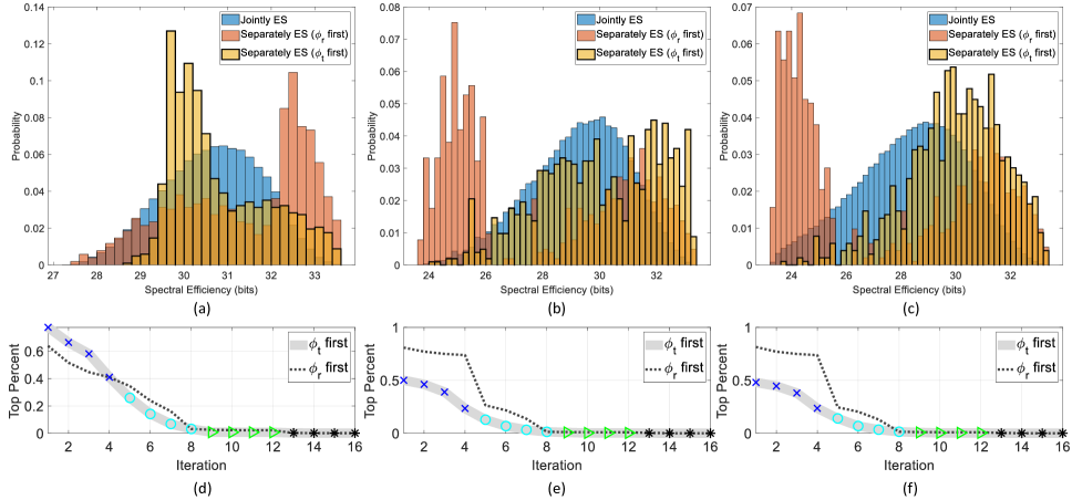
Figure 4: Histograms of the SE achieved by joint ES and separate ES in three different positions: (a) $(1,1,1)\,\lambda_{\rm H}$, (b) $(5,5,5)\,\lambda_{\rm H}$, and (c) $(10,10,10)\,\lambda_{\rm H}$. (e)–(f) depict the corresponding trajectories of the BG algorithm. The achieved SEs are marked by $\times$, $\circ$, $\triangleright$, and $\ast$ for the iterations $[1:N_{\rm c}]$, $[N_{\rm c}+1:2N_{\rm c}]$, $[2N_{\rm c}+1:3N_{\rm c}]$, and $[3N_{\rm c}+1:4N_{\rm c}]$.

First, we demonstrate the optimality properties of ${\boldsymbol{\phi}}_{\rm t}$ and ${\boldsymbol{\phi}}_{\rm r}$ for Structure 2. For this study, we set $M=N_{\rm 1}=N_{\rm 2}=N_{\rm c}=4$. All channel matrices are generated based on

$${\bf H}_{\ast}=\sqrt{\frac{1}{\kappa_{\ast}+1}}{\bf H}_{{\rm iid},\ast}+\sqrt{\frac{\kappa_{\ast}}{\kappa_{\ast}+1}}{\bf H}_{{\rm LOS},\ast},$$ (37)

where ${\ast}\in\{1,{\rm c},{\rm p}\}$. For ease of notation, we usually omit the subscript “${\ast}$”, implying that the descriptions apply to all the concerned cases. Here, ${\bf H}_{\rm iid}$ represents the NLOS part of the channel with entries being i.i.d. ${\cal N}_{{\mathbb{C}}}(0,1)$-distributed. ${\bf H}_{\rm LOS}$ represents the LOS part of the channel, with entry $[{\bf H}_{\rm LOS}]_{n,m}$ modeling the channel response between transmit antenna $m$ and receive antenna $n$ as

$$[{\bf H}_{\rm LOS}]_{n,m}=e^{-j2\pi\frac{d_{n,m}}{\lambda}},$$ (38)

where $\lambda$ is the wavelength and $d_{n,m}$ denotes the distance between transmit antenna $m$ and receive antenna $n$. The $\kappa$-factor determines the gain division between the LOS and NLOS parts. We use the SNR to reflect signal quality and thus omit the large-scale fading effect for conciseness.

Pr-UE is positioned at the origin, while the BS is located at $[100,100,100]\,\lambda_{\rm L}$. The Co-UE is considered at three different positions relative to Pr-UE: $(1,1,1)\,\lambda_{\rm H}$, $(5,5,5)\,\lambda_{\rm H}$, and $(10,10,10)\,\lambda_{\rm H}$. Note that these locations have been normalized with respect to their operational wavelengths. The varying positions of Co-UE relative to Pr-UE result in a transition of the channel matrix ${\bf H}_{{\rm LOS},{\rm p}}$ from full rank (i.e., near-field) to rank-1 (i.e., far-field).

We consider a 3-bit element phase resolution (i.e., $Q=8$ levels) for each DPS. The SNR is set at 20 dB, measured based on Pr-UE. The $\kappa$-factors are set as $\kappa_{1}=\kappa_{\rm c}=0$, and $\kappa_{\rm p}=\infty$. Thus, ${\bf H}_{1}$ and ${\bf H}_{\rm c}$ are completely composed of i.i.d. Rayleigh fading channels, and ${\bf H}_{\rm p}$ is completely composed of the LOS part.

Fig. 4 shows the histograms of the SE achieved by exhausting all combinations of $({\boldsymbol{\phi}}_{\rm t},{\boldsymbol{\phi}}_{\rm r})$, totaling $8^{N_{\rm c}}\times 8^{N_{\rm c}}$ combinations, referred to as joint exhaustive search (ES). We also show the histograms of SE achieved by separately exhausting all combinations of ${\boldsymbol{\phi}}_{\rm t}$ and ${\boldsymbol{\phi}}_{\rm r}$, totaling $2\times 8^{N_{\rm c}}$ combinations, referred to as separate ES. Separate ES explores only a subset of the combinations available to joint ES. For separate ES, we consider two strategies:

• ${\boldsymbol{\phi}}_{\rm t}$ first: Perform ES first on ${\boldsymbol{\phi}}_{\rm t}$ and then on ${\boldsymbol{\phi}}_{\rm r}$.

• ${\boldsymbol{\phi}}_{\rm r}$ first: Perform ES first on ${\boldsymbol{\phi}}_{\rm r}$ and then on ${\boldsymbol{\phi}}_{\rm t}$.

The figure shows that in all three cases with different positions of Co-UE, joint ES and separate ES achieve the same optimal SE, while separate ES enjoys much lower complexity than joint ES. This characteristic verifies our finding in Theorem 1. Additionally, the exhaustive order is irrelevant to the final optimal result. However, ${\boldsymbol{\phi}}_{\rm r}$ first is preferred in Fig. 4(a), where the histograms of separate ES mostly appear in a higher SE region than those of joint ES and ${\boldsymbol{\phi}}_{\rm t}$ first. Conversely, ${\boldsymbol{\phi}}_{\rm t}$ first is preferred in Figs. 4(b) and 4(c). This demonstrates that whether ${\boldsymbol{\phi}}_{\rm t}$ or ${\boldsymbol{\phi}}_{\rm r}$ is first depends on whether the corresponding channel is dominated by a single strong path. For example, in Fig. 4(a), ${\bf H}_{\rm p}$ is full rank, so ${\boldsymbol{\phi}}_{\rm t}$ first does not play a critical enhancement role compared to the other two cases.

In Figs. 4(d), 4(e), and 4(f), we show the averaged trajectory of the BG algorithm, averaged over 10,000 trials of random channels. The vertical axis represents the top percentile, indicating that if a point is at the 0.1 top percentile, it has reached the top 10% of the SE achieved by the separate ES. We observe that the SE can effectively increase with the iterations of BG, eventually achieving optimal results. Notably, after the first $N_{\rm c}$ iterations, following its preference for ${\boldsymbol{\phi}}_{\rm t}$ or ${\boldsymbol{\phi}}_{\rm r}$ order (e.g., BG for ${\boldsymbol{\phi}}_{\rm t}$ first), it already reaches the top 20% of the SE. After completing the first $2N_{\rm c}$ iterations (whether ${\boldsymbol{\phi}}_{\rm t}$ or ${\boldsymbol{\phi}}_{\rm r}$ first), it typically achieves the top 1% of the SE. Further iterations result in minor improvements but make ${\boldsymbol{\phi}}_{\rm t}$ and ${\boldsymbol{\phi}}_{\rm r}$ converge to nearly the optimal solution. The trajectories between ${\boldsymbol{\phi}}_{\rm t}$ first and ${\boldsymbol{\phi}}_{\rm r}$ first again demonstrate the advantage of employing the ${\boldsymbol{\phi}}_{\rm t}$ first strategy in the cases with a single strong path ${\bf H}_{\rm p}$ (i.e., Fig. 4(e) and Fig.  4(f)), although both strategies eventually reach the same optimal solution.

IV-B Advantage of UE-CoMIMO

Next, we discuss the advantages of the UE-CoMIMO system between structures 1 and 2. Unless otherwise specified, the scenarios and parameters are set the same as those in the previous subsection.

Initially, we focus on Structure 2. We consider the phase resolution at different levels: infinite, and $Q=32$, $16$, and $2$ levels. For finite resolution cases, we apply either ES for the optimal solution of $({\boldsymbol{\phi}}_{\rm t},{\boldsymbol{\phi}}_{\rm r})$ or the more efficient BG algorithm. For infinite phase resolution, we use SDP to solve problems (P2-1) and (P2-2), denoted as optimal (continuous) phases. We also examine the case where ${\boldsymbol{\phi}}_{\rm r}$ and ${\boldsymbol{\phi}}_{\rm t}$ allow amplitude adjustments. Here, the maximal SE is achieved by setting ${\boldsymbol{\phi}}_{\rm t}={\bf v}_{{\rm H}{\rm p}}$ and ${\boldsymbol{\phi}}_{\rm r}={\bf u}_{\widetilde{\rm H}{\rm c}}$, referred to as optimal beamforming. For UE-CoMIMO, we refer to Structure 1 with ${\boldsymbol{\Phi}}_{\rm s1}={\bf I}_{N_{\rm c}}$. To ensure fair comparison between structures 1 and 2, we have normalized the power of both structures in all cases with ${\sf tr}({\boldsymbol{\Phi}}_{\rm s})=N_{\rm c}$, though we do not explicitly state the normalization factors for conciseness.

Fig. 5 shows the SEs for all the mentioned algorithms in three different Co-UE positions: (a) $(1,1,1)\,\lambda_{\rm H}$, (b) $(5,5,5)\,\lambda_{\rm H}$, and (c) $(10,10,10)\,\lambda_{\rm H}$. The UE-CoMIMO of both structures significantly outperforms Pr-UE alone. In Structure 1, all algorithms with either optimal beamforming or suboptimal continuous or discrete phases provide comparable results. The random setting of phases is not competitive, while the BG algorithm is attractive as it closely approximates the optimal beamforming even with only two phase levels ($Q=2$). When Co-UE is positioned at $(1,1,1)\,\lambda_{\rm H}$, ${\bf H}_{\rm p}$ is full rank. Fig. 5(a) shows that Structure 1 is more beneficial even without optimizing its phase state. Structure 2 demonstrates its advantage over Structure 1 in Figs. 5(b) and 5(c), showing its superiority when ${\bf H}_{\rm p}$ approaches rank-1 channels.

Next, we focus on Structure 1. Fig. 6 shows the SEs through the ES and BG algorithms. Adjusting phases brings minor gains to Structure 1. Structure 1 with phase adjustments appears to gain more when ${\bf H}_{\rm p}$ approaches rank-1 channels. However, comparing Figs. 5(c) and 6(c), Structure 2 with optimal phases remains superior to Structure 1 with optimal phases. Conversely, comparing Figs. 5(a) and 6(a), Structure 1 without phase adjustments is already superior to Structure 2 with optimal phases.

We also examine all the above characteristics over various $\kappa$-factors, though these results are not shown here due to space limitations. Consequently, we find that the choice between Structures 1 and 2 depends on the specific use case. For scenarios where ${\bf H}_{\rm p}$ is close to full rank, Structure 1 is preferred. In contrast, for scenarios where ${\bf H}_{\rm p}$ approaches rank-1, Structure 2 is more suitable. Phase optimization offers minor gains for Structure 1 but becomes crucial for Structure 2.

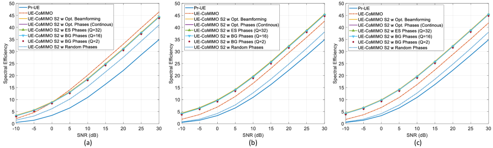
Figure 5: SEs of various algorithms, particularly for Structure 2, in three different positions: (a) $(1,1,1)\,\lambda_{\rm H}$, (b) $(5,5,5)\,\lambda_{\rm H}$, and (c) $(10,10,10)\,\lambda_{\rm H}$. The algorithms include the optimal beamforming, the SDR for the optimal (continuous) phases, ES for discrete phases, and the BG algorithm for discrete phases under $Q=32$, $16$, and $2$ levels.

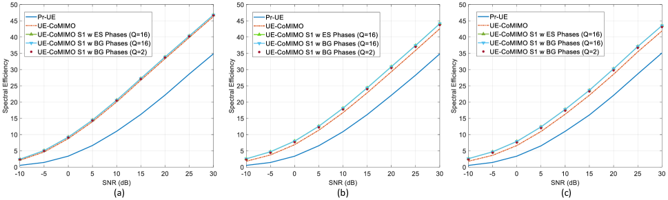
Figure 6: SEs of various algorithms, particularly for Structure 1, n three different positions: (a) $(1,1,1)\,\lambda_{\rm H}$, (b) $(5,5,5)\,\lambda_{\rm H}$, and (c) $(10,10,10)\,\lambda_{\rm H}$. The algorithms include ES for discrete phases, and the BG algorithm for discrete phases under $Q=16$ and $2$ levels.

IV-C Evaluation Through Ray-Tracing in Indoor Scenario

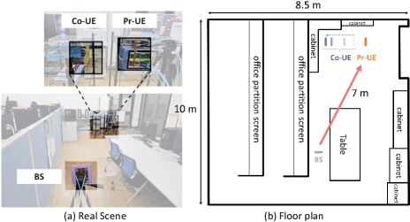
Figure 7: The testing scenario (a) real scene; (b) floor plan

TABLE II: Parameters of the experiment.

Environment	Indoor Office	Boston
Carrier Freq.	$f_{\rm L}=3.65$ GHz	$f_{\rm L}=3.5$ GHz
	$f_{\rm H}=7.65$ GHz	$f_{\rm L}=7$ GHz
Bandwidth	100 MHz
FFT, Subcarriers	2048/1620
Sampling Rate	122.88 Msps
Antenna Conf.	$M=4$	$M=8$
	$N_{\rm c}=4$	$N_{\rm c}=4$
	$N_{1}=N_{2}=2$	$N_{1}=N_{2}=2$
BS and Pr-UE Distance	$\sim 7$ m	$1.3-587.6$ m
Pr-UE and Co-UE Distance	0.03, 0.05,	0.05 m
	0.1, 0.2, $\ldots$ , 0.5 m
Tx Power	-12 dBm	0 dBm
Noise Power	-94 dBm
LNA Gain	20 dB
BS Height	2 m	15 m
UE Height	1.2 m
PS Opt. Alg.	BG (4 levels)

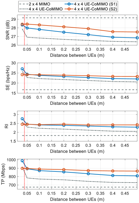
Figure 8: Performances with varying distances between Co-UE and Pr-UE.

To gain a more practical understanding of the use cases, we conducted ray-tracing simulations. Compared to the statistical channel models used in the previous subsection, the ray-tracing approach better captures the geometric properties of the channels. We first considered an indoor laboratory scenario in the NSYSU Electrical and Computer (EC) Engineering Building, as depicted in Fig.  7. Section V will describe over-the-air (OTA) tests performed in the same setting. The room dimensions are 10 m in length, 8.5 m in width, and 2.2 m in height. The BS and Pr-UE were positioned as shown in Fig. 7, with Co-UE placed near Pr-UE at varying distances.

The frequency bands considered are $f_{\rm L}$ at 3.65 GHz, similar to the current 5G NR commercial network, and $f_{\rm H}$ at 7.65 GHz. Using Wireless InSite^®, we generated the propagation channels between the BS and Pr-UE, BS and Co-UE, and Co-UE and Pr-UE. The system employs a 5G NR MIMO-OFDM waveform with a 100 MHz bandwidth and a subcarrier spacing of 60 kHz, adhering to the 5G NR frame structure. The BS is equipped with four antennas, while the Pr-UE is equipped with four antennas—two antennas for $f_{\rm L}$ and two for $f_{\rm H}$. Co-UE is equipped with four antennas for both frequency bands. Table II summarizes the system parameters.

Fig. 8 illustrates the performance variations with changing distances between Co-UE and Pr-UE. We evaluated several metrics, including SNR (in dB), spectral efficiency (SE in bps/Hz), rank indicator (RI), and throughput (TP in Mbps) for both the 2R4T MIMO (Pr-UE only) and 4T4R UE-CoMIMO systems. The SNR is averaged across all receiving antennas in the linear domain. SE is calculated based on (27). TP is evaluated following the 3GPP TR 38.306 [22], where the BS applies precoding to determine the Channel Quality Indicator (CQI) and RI according to the 5G NR standard.

When comparing the performance of Pr-UE only (gray dashed line) with UE-CoMIMO (gray dash-dotted line), we observe that all metrics, except for SNR, are generally better for UE-CoMIMO. The SNR decreases as the distance between Co-UE and Pr-UE increases due to increased path loss. In the Pr-UE-only configuration, two Rx antennas operate at $f_{\rm L}$, while in the UE-CoMIMO configuration, two Rx antennas operate at $f_{\rm L}$ and two at $f_{\rm H}$. The SNR at $f_{\rm L}$ remains unaffected by the distance between Co-UE and Pr-UE, indicating that the variations in UE-CoMIMO SNR are due to differences in SNR at $f_{\rm H}$. A decrease in the averaged SNR for UE-CoMIMO therefore reflects lower SNRs at $f_{\rm H}$. This outcome is expected because free space path loss at $f_{\rm H}$ (7.65 GHz) exceeds 30 dB at a distance of 0.1 m, and the 20 dB gain from the LAN cannot fully compensate for this loss. Despite the lower average SNRs, UE-CoMIMO achieves higher SE compared to Pr-UE only. The RI for Pr-UE only is below two, while UE-CoMIMO can exceed a rank of two due to the additional channels provided by Co-UE.

Notably, when the Co-UE and Pr-UE are in close proximity, the performance gains in SE, RI, and TP for UE-CoMIMO are significant. At short distances, the channel matrix ${\bf H}_{\rm p}$ approaches full-rank, leading to notable improvements. However, as the distance between Co-UE and Pr-UE exceeds the Fraunhofer distance—indicated by the red dashed vertical line in Fig.  8—the channel ${\bf H}_{\rm p}$ quickly degenerates to a rank-one channel, resulting in diminished performance gains. Interestingly, in the real OTA tests described in V, the distance at which ${\bf H}_{\rm p}$ degenerates to a rank-one channel is not as short. One potential reason for this discrepancy is that, in our ray-tracing simulations, we limited the maximum number of path reflections and edge diffractions in Wireless InSite^® to reduce computation time. Moreover, the real-world scenario likely includes more scatterers than those considered in the simulation, which could help maintain higher-rank channels over longer distances.

Considering optimal phase settings under Structure 1 and Structure 2, the BG algorithm is used to optimize phases. Generally, performance improves with phase optimization compared to UE-CoMIMO alone. Structure 2 shows significant SNR improvements over Structure 1. At a 0.03 m distance, SE, rank, and throughput for Structure 2 are lower than for UE-CoMIMO, as Structure 2 reduces channel ${\bf H}_{2}$ to rank-one. However, as the distance increases, the benefits of Structure 2 become more apparent. These findings are consistent with our earlier observations.

IV-D Evaluation Through Ray-Tracing in Outdoor Scenario

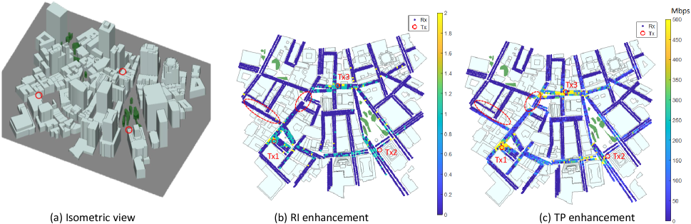
Figure 9: (a) Isometric view of a section of downtown Boston in Wireless InSite [23]. (b) Enhancement in terms of RI. (c) Enhancement in terms of TP.

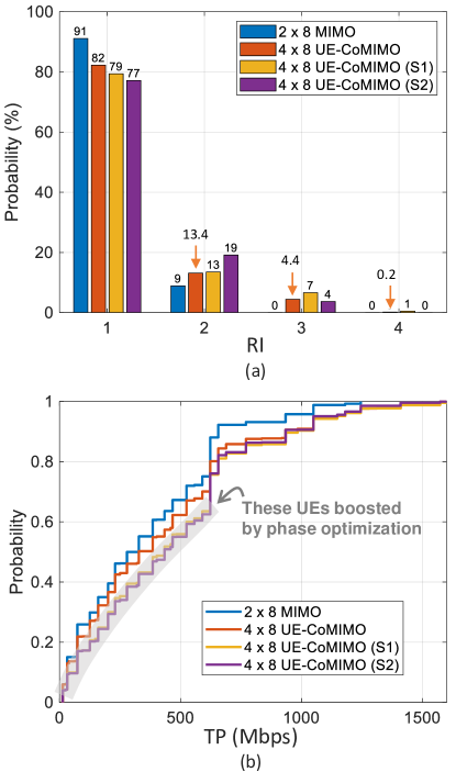
Figure 10: (a) Probability distribution of the RI used. (b) CDF of the TP.

To broaden our perspective, we next conducted ray-tracing simulations for UE-CoMIMO in an outdoor area based on a section of downtown Boston. The building and foliage geometry were imported from a high-resolution shapefile developed and released by Remcom [23], as shown in Fig. 9(a). Each Tx represents a BS (marked as “$\circ$” in Fig. 9(a)) and uses a $1\times 8$ uniform linear array with half-wavelength spacing between antenna elements, with each antenna element being isotropic. The antenna configurations for the Co-UE and Pr-UE are the same as those described in the previous subsection. Other system parameters are summarized in Table II. The UE is uniformly placed in the outdoor x-y grid with 5 m spacing between adjacent points, resulting in 2,454 UEs in the outdoor area. The height of all user grids is 1.2 m. There are three BSs operating on different frequency channels around 3.5 GHz. The UE connects to the BS with the strongest SNR.

We evaluated the TP in Mbps for the 2R8T MIMO (Pr-UE only) and 4R8T UE-CoMIMO systems, with precoding applied by the BS to determine the CQI and RI as per the 5G NR standard. The rank number and TP of the 4R8T UE-CoMIMO system are expected to be higher than those of the 2R8T MIMO system. Figs. 9(b) and 9(c) illustrate the enhancement in terms of RI and TPP, respectively. We observe that the 4R8T UE-CoMIMO system boosts the rank number, particularly when the UE is close to the BS. It typically adds one additional rank across most areas, with two additional ranks being common in certain regions. However, the rank is not enhanced when the UE is far from the BS. The rank enhancement is also minimal for UEs around Tx2, as this area is an open garden with fewer available propagation paths. Despite the limited rank enhancement in certain areas, such as the garden and the regions marked by red dotted circles, UE-CoMIMO still significantly boosts TP. This indicates that even when spatial multiplexing gains are limited, UE-CoMIMO improves performance through other mechanisms, such as better signal quality and increased diversity.

In Fig. 10(a), the probability distribution of the RI based on ray-tracing simulations is presented. In the 2R8T MIMO system, 91% of UEs have a rank of 1, while only 9% can support up to rank 2. When using the 4R8T UE-CoMIMO, the proportion of rank 1 UEs decreases to 82%. With Structure 1 and Structure 2, this proportion further reduces to 79% and 77%, respectively. These reductions indicate a transition of UEs to higher ranks. Structure 2 supports up to 3 ranks, while Structure 1 and UE-CoMIMO can support up to rank 4. Structure 1 exhibits a higher probability of achieving rank 4, indicating that phase shifter adjustments can further enhance spatial multiplexing gains. Fig. 10(b) illustrates the corresponding cumulative distribution function (CDF) of the TP. The CDFs of TP for Structure 1 and Structure 2 are similar and higher than those for UE-CoMIMO and 2R8T MIMO. Compared to UE-CoMIMO without phase optimization, over 60% of UEs experience performance improvement due to phase optimization.

V Implementation and Tests

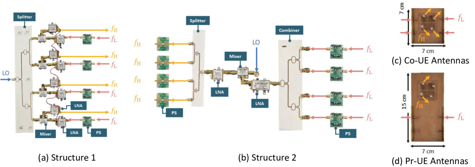
Figure 11: Hardware configurations of (a) Structure 1 and (b) Structure 2, following the architectures depicted in Fig. 3. Antenna configurations for (c) Co-UE and (d) Pr-UE are shown.

In this section, we evaluate the performance and feasibility of the UE-CoMIMO system through OTA testing. The test environment, configuration, and frequency bands for $f_{\rm L}$ and $f_{\rm H}$ are aligned with those used in the ray-tracing simulations for the indoor scenario discussed in Section IV-C. We employ a 5G NR MIMO-OFDM system, utilizing the same parameters listed in Table II. The system adheres to 5G NR standards, ensuring that the experimental performance and characteristics of the UE-CoMIMO system are applicable within the context of 5G communications.

V-A Device and Implementation

Following the architecture shown in Fig. 3, we implemented both Structure 1 and Structure 2, as shown in Fig. 11. The specifications of the components used are listed in Table I. Co-UE is equipped with four antennas on the phone’s side edge for the $f_{\rm L}$ band and another four antennas on the back cover for the $f_{\rm H}$ band, as shown in Fig. 11(c). These antennas are designed to fit within the form factor of a 5G smartphone, considering space restrictions. The side edge antennas at the low mid-band are nearly omnidirectional, while the back cover antennas at the upper mid-band are slightly directional. We utilize the MAP-010144 digital phase shifter (DPS) for the $f_{\rm L}$ band and the TGP2105-SM DPS for the $f_{\rm H}$ band. Both are 6-bit DPSs that enable a phase shift ranging from 0 to 360 degrees in increments of 5.625 degrees. However, as discussed in Section IV-B, the performance with $Q=2$ is already close to that with continuous phase. Considering the performance and complexity trade-off, we adopt four phases ($Q=4$), i.e., $0,90,180,270$ degrees. The control link between Pr-UE and Co-UE is established through a half-duplex Bluetooth connection.

To conduct the test, we also need a transmitter and receiver to serve as the BS and Pr-UE, respectively. For the BS, we employ four one-port Rohde & Schwarz (R&S) vector signal generators, SGT100A, which are connected to four transmit antennas. Multiple spatial-stream 5G OFDM signals are transmitted via precoding in the 3.6-3.7 GHz band over the air. For Pr-UE, we receive the signals at $f_{\rm L}$ and $f_{\rm H}$ using two mobile 5G antennas and two upper mid-band antennas, as shown in Fig. 11(d). The received signals from the four antennas (two at $f_{\rm L}$ and two at $f_{\rm H}$) are downconverted to the baseband using a four-port R&S digital oscilloscope, specifically the RTP164.

The receiver downconverts the received signals to the baseband, and then the baseband signals are subsequently processed using a C program on a personal computer. Synchronization is performed using 5G synchronization signal blocks. By performing channel estimation and MIMO detection, we calculate the averaged SNR (dB), SE (bps/Hz), RI, and TP (bps) of the 4T4R MIMO and 4T8R UE-CoMIMO systems.

V-B Results

TABLE III: Experiment results of Pr-UE only and UE-CoMIMO for Structure 1.

	Pr-UE Only				Structure 1 (Initial PS)				Structure 1 (BG PS)
Co-UE Dist. (m)	SNR (dB)	SE (bps/Hz)	RI (#)	TP (Mbps)	SNR	SE	RI	TP	SNR	SE	RI	TP
0.03	24.73	15.12	1.39	503.4	29.06	30.03	3.00	1275.2	30.33	30.77	3.00	1286.9
0.5					27.12	28.39	2.94	1024.2	26.25	28.89	3.00	1044.6
1					24.77	24.91	2.03	870.21	24.10	26.10	3.00	1151.8

TABLE IV: Experiment results of Pr-UE only and UE-CoMIMO for Structure 2.

	SNR of Rx1 at $f_{\rm H}$		SNR of Rx2 at $f_{\rm H}$		Structure 2 (Initial PS)				Structure 2 (BG PS)
Co-UE Dist. (m)	Initial	BG	Initial	BG	SNR	SE	RI	TP	SNR	SE	RI	TP
0.03	26.18	33.59	22.37	30.50	23.22	20.78	2.25	755.2	29.63	23.34	2.97	835.7
0.5	6.66	18.53	3.95	13.17	23.37	17.60	1.65	533.4	23.78	20.71	3.00	723.1
1	3.02	9.88	-1.69	10.56	23.41	17.31	1.99	629.9	23.52	19.37	2.03	632.4

We conducted experimental measurements in an indoor laboratory of the NSYSU EC Engineering Building to assess the UE-CoMIMO system, as shown in Fig. 7. The Co-UE was placed at varying distances of 0.03 m, 0.5 m, and 1 m from Pr-UE. The distance of 0.03 m mimics a use case where a portable charger serves as Co-UE, while distances of 0.5 m and 1 m mimic use cases where a wearable device serves as Co-UE. These scenarios result in a full-rank channel and rank-defective channels of ${\bf H}_{\rm p}$, respectively.

Without UE-CoMIMO, Pr-UE can only support two spatial streams. We started with Structure 1 in the experiment. According to our calculations, the LNAs in each link of the frequency translator can provide about 40 dB gain. Note that the free space path loss is 50.11 dB for a distance of 1 m at $f_{\rm H}=7.65$ GHz. Therefore, the LNA cannot compensate for the path loss at $f_{\rm H}$ in all cases. The corresponding results are summarized in Table III.

In most cases (except for the 0.03 m scenario), the SNRs of UE-CoMIMO are decreased, demonstrating that the SNRs at $f_{\rm H}$ are lower than those at $f_{\rm L}$. This result is expected, as the link between Co-UE and Pr-UE operates at a high frequency and suffers from higher path loss. However, even with low SNRs and without performing BG for PSs, the UE-CoMIMO still provides significant enhancements in SE compared to Pr-UE, which has an SE of only 15.12 bps. Specifically, in the 0.03 m case, the SE is remarkably boosted to 30.03 bps because the two additional channels from Co-UE also bring rank enhancement. In the 0.5 m and 1 m cases, the SEs are significantly boosted even though the averaged SNR is lower than that in Pr-UE. Comparing the RI results with those in Fig. 8 from the ray-tracing simulations, the rank number in the experiment is more optimistic than that in the ray-tracing simulations. This indicates that more scatters are available in practical use cases, making the full-rank MIMO link between Co-UE and Pr-UE more likely to be established.

When the BG algorithm is applied, the SEs can be further boosted. Specifically, in the 0.03 m case, both the SNR and SE are further boosted. In the 0.5 m case, the SE is boosted while the SNR remains comparable to the case without BG. This is expected because the BG algorithm for Structure 1 targets increasing the SE rather than the SNR, leading to an increase in RI. A similar characteristic is observed in the 1 m case.

Next, we consider Structure 2. Because we do not implement a mechanism to control the gain of the LNA due to low complexity, the antenna output power of Structure 1 and Structure 2 are not identical. In fact, the output power of Structure 2 is lower than that of Structure 1 because Structure 2 has an additional high-frequency PS. Therefore, performance comparisons between Structure 1 and Structure 2 are not completely fair. Thus, we primarily compare the performances before BG and after BG within Structure 2. The SNRs of the two antennas for $f_{\rm H}$ at Pr-UE are shown in Table IV. We find that the SNRs of $f_{\rm H}$ are significantly boosted after BG for all three distances. This result is reasonable because the BG algorithm for Structure 2 primarily boosts the SNRs for the $f_{\rm H}$ channel, effectively creating four channels for the receiver. This leads to improvements in SE, RI, and TP. Recall that with Structure 1, the SE does not significantly boost due to BG. However, with Structure 2, the SEs after applying BG are significantly boosted for all three cases. This observation is consistent with our results from the simulations in Section IV-B.

VI Conclusion

This paper has analyzed the performance of the UE-CoMIMO system, which utilizes multiple fixed or portable devices within a personal area to create a virtually expanded antenna array. Our analytical results demonstrate that UE-CoMIMO significantly enhances the system’s effective channel response without the need for phase shifter optimization, with further improvements possible through the optimized integration of phase shifters into the portable devices, categorized as Structures 1 and 2. Our findings indicate that the preferred structure depends on the specific use case. For scenarios where the relay channel exhibits near full-rank characteristics, such as when a wearable device serves as Co-UE, Structure 1 is the preferred choice. Conversely, when the relay channel approaches rank-1 characteristics, such as when a customer premise equipment serves as Co-UE, Structure 2 is more suitable. While phase optimization provides minimal benefits for Structure 1, it is crucial for maximizing the performance of Structure 2. We also implemented these collaborative devices and validated our observations in a real 5G environment. Our testing results suggest that in practical use cases, the presence of more scatterers increases the likelihood of establishing a full-rank MIMO link between Co-UE and Pr-UE.

References

- [1] W. Chen, X. Lin, J. Lee, A. Toskala, S. Sun, C. F. Chiasserini, and L. Liu, “5G-Advanced toward 6G: Past, present, and future,” IEEE J. Sel. Areas Commun., vol. 41, no. 6, pp. 1592–1619, 2023.
- [2] X. Lin, “The bridge toward 6G: 5G-Advanced evolution in 3GPP Release 19,” arXiv:2312.15174, 2023. [Online]. Available: https://arxiv.org/abs/2312.15174
- [3] H. Jin, K. Liu, M. Zhang, L. Zhang, G. Lee, E. N. Farag, D. Zhu, E. Onggosanusi, M. Shafi, and H. Tataria, “Massive MIMO evolution toward 3GPP Release 18,” IEEE J. Sel. Areas Commun., vol. 41, no. 6, pp. 1635–1654, 2023.
- [4] C.-K. Wen, L.-S. Tsai, A. Shojaeifard, P.-K. Liao, K.-K. Wong, and C.-B. Chae, “Shaping a smarter electromagnetic landscape: IAB, NCR, and RIS in 5G standard and future 6G,” vol. 8, no. 1, pp. 72–78, 2024.
- [5] E. Björnson, C.-B. Chae, R. W. H. Jr., L. T. Marzetta, A. Mezghani, L. Sanguinetti, F. Rusek, M. R. Castellanos, D. Jun, and O. T. Demir, “Towards 6G MIMO: Massive spatial multiplexing, dense arrays, and interplay between electromagnetics and processing,” arXiv:2401.02844, 2024. [Online]. Available: https://arxiv.org/abs/2401.02844
- [6] K.-L. Wong, S.-E. Hong, and W.-Y. Li, “Low-profile four-port MIMO antenna module based 16-port closely-spaced 2 × 2 module array for 6g upper mid-band mobile devices,” IEEE Access, vol. 11, pp. 110 796–110 808, 2023.
- [7] L.-S. Tsai, S.-L. Shih, P.-K. Liao, and C.-K. Wen, “MIMO evolution toward 6G: End-user-centric collaborative MIMO,” IEEE Commun. Mag., vol. 62, no. 7, pp. 104–110, 2024.
- [8] RWS-230111, “Device collaborative Tx and Rx,” MediaTek Inc., 3GPP RAN Rel-19 workshop, Taipei, TW, Jun. 2023.
- [9] D. W. K. Ng, M. Breiling, C. Rohde, F. Burkhardt, and R. Schober, “Energy-efficient 5G outdoor-to-indoor communication: SUDAS over licensed and unlicensed spectrum,” IEEE Trans. Wireless Commun., vol. 15, no. 5, pp. 3170–3186, 2016.
- [10] O. D. J. Sánchez and J. I. Alonso, “A two-hop MIMO relay architecture using LTE and millimeter wave bands in high-speed trains,” IEEE Trans. Veh. Technol., vol. 68, no. 3, pp. 2052–2065, 2019.
- [11] C.-W. Chen, W.-C. Tsai, L.-S. Tsai, and A.-Y. Wu, “Relay-assisted carrier aggregation (RACA) uplink system for enhancing data rate of extended reality (XR),” arXiv:2407.01912, 2024. [Online]. Available: https://arxiv.org/abs/2407.01912
- [12] X. Xie, C. He, X. Ma, F. Gao, Z. Han, and Z. J. Wang, “Joint precoding for active intelligent transmitting surface empowered outdoor-to-indoor communication in mmWave cellular networks,” IEEE Trans. Wireless Commun., vol. 22, no. 10, pp. 7072–7086, 2023.
- [13] M. H. N. Shaikh, V. A. Bohara, A. Srivastava, and G. Ghatak, “An energy efficient dual IRS-aided outdoor-to-indoor communication system,” IEEE Systems Journal, vol. 17, no. 3, pp. 3718–3729, 2023.
- [14] C. Chen, Y. Niu, B. Ai, R. He, Z. Han, Z. Zhong, N. Wang, and X. Su, “Joint design of phase shift and transceiver beamforming for intelligent reflecting surface assisted millimeter-wave high-speed railway communications,” IEEE Trans. Veh. Technol., vol. 72, no. 5, pp. 6253–6267, 2023.
- [15] W. Tang, J. Y. Dai, M. Z. Chen, K.-K. Wong, X. Li, X. Zhao, S. Jin, Q. Cheng, and T. J. Cui, “MIMO transmission through reconfigurable intelligent surface: System design, analysis, and implementation,” IEEE J. Sel. Areas Commun., vol. 38, no. 11, pp. 2683–2699, 2020.
- [16] C. R. J. Roger A. Horn, Matrix Analysis. Cambridge University Press, New York, 1990.
- [17] C. F. V. L. Gene H. Golub, Matrix Computations. 3rd ed. The Johns Hopkins University Press, 1996.
- [18] L. Zhu, X. Peng, and H. Liu, “Rank-one perturbation bounds for singular values of arbitrary matrices,” J. Inequal. Appl., no. 138, 2019.
- [19] Q. Wu and R. Zhang, “Intelligent reflecting surface enhanced wireless network: Joint active and passive beamforming design,” in 2018 IEEE Global Communications Conference (GLOBECOM), 2018, pp. 1–6.
- [20] S. Zhang and R. Zhang, “Capacity characterization for intelligent reflecting surface aided MIMO communication,” IEEE J. Sel. Areas Commun., vol. 38, no. 8, pp. 1823–1838, 2020.
- [21] D.-M. Chian, C.-K. Wen, C.-H. Wu, F.-K. Wang, and K.-K. Wong, “A novel channel model for reconfigurable intelligent surfaces with consideration of polarization and switch impairments,” IEEE Transactions on Antennas and Propagation, vol. 72, no. 4, pp. 3680–3695, 2024.
- [22] User Equipment (UE) Radio Access Capabilities. 3GPP TR 38.306 V16.3.0, Jan. 2021.
- [23] Remcom, Inc. Throughput of a 5G New Radio FD-MIMO System in an Urban Area Using Custom Beamforming.