CSPS: A Communication-Efficient Sequence-Parallelism based Serving System for Transformer based Models with Long Prompts

Abstract

Long-sequence generative large-language model (LLM) applications have become increasingly popular. In this paper, through trace-based experiments, we found that the existing method for long sequences results in a high Time-To-First-Token (TTFT) due to sequential chunk processing, long Time-Between-Tokens (TBT) from batching long-sequence prefills and decodes, and low throughput due to constrained key-value cache (KVC) for long sequences. To address these issues, we propose two Sequence-Parallelism (SP) architectures for both tensor parallelism (TP) and non-TP. However, SP introduces two challenges: 1) network communication and computation become performance bottlenecks; 2) the latter two issues above are mitigated but not resolved, and SP’s resultant KV value distribution across GPUs still requires communication for decode, increasing TBT. Hence, we propose a Communication-efficient Sparse Attention (CSA) and communication-computation-communication three-phase pipelining. We also propose SP-based decode that processes decode separately from prefill, distributes KV values of a request across different GPUs, and novelly moves Query (Q) values instead of KV values to reduce communication overhead. These methods constitute a Communication-efficient Sequence-Parallelism based LLM Serving system (CSPS). Our trace-driven evaluation demonstrates that CSPS improves the average TTFT, TBT and response time by up to 7.5$\times$, 1.92$\times$ and 9.8$\times$ and improves the prefill and decode throughput by 8.2$\times$ and 5.2$\times$ while maintaining the accuracy compared to Sarathi-Serve. We distributed our source code.

1 Introduction

In recent years, the transformer-based generative large language models (LLMs) scaled up towards billions and even trillions of parameters to improve model capabilities, which have been well exemplified by the GPT model series [1, 2, 3], OPT [4], and Llama series [5, 6]. As the models’ contextual understanding and ability to handle longer and more complex text inputs have been increasingly enhanced, the allowable input sequence length has been substantially increased, ranging from 4K to 1M tokens [7, 8, 9, 10, 11]. For example, applications such as book summarization [12, 13, 14], document classification [15, 16], and coding assistance [17] require a longer or unlimited sequence length to fully understand the extended context. Some long-sequence applications, such as coding assistance, require short response time (e.g., in seconds). However, through experimental measurements, we made Observation (O):

• The existing serving system that handles long sequences, Sarathi-Serve [18], generates long Time-To-First-Token (TTFT) (in minutes) due to sequential chunk processing, high Time-Between-Token (TBT) (e.g., 6 seconds) from batching long-sequence prefills and decodes, and low throughput due to small batch size caused by constrained KV cache size and long sequences.

To address the problems, we propose sequence parallelism (SP) architectures that partition a long input sequence and use multiple GPUs to process the partitions in parallel.

(1) SP-based Prefil. We propose two SP architectures: SP-NTP for Non-Tensor Parallelism and SP-TP for Tensor Parallelism. SP-NTP lets each GPU process one sequence partition (SPT), then distributes the Query-Key-Value (QKV) of different heads across GPUs via the all-to-all (A2A) communication for self-attention computations, and finally uses another A2A to collect the self-attention output of each partition to a separate GPU. On the other hand, SP-TP uses all-gather to collect SPTs into each GPU for self-attention computations followed by a post-self-attention linear transformation, and then uses the reduce-scatter communication to combine and distribute the linear outputs so that the linear output of each partition is in a separate GPU. We batch the last SPT with other small prefill tasks to improve throughput.

However, through experimental measurements on the two SP architectures, we the following observations:

• The network communication and attention computation may become bottlenecks.

• Processing decodes along with the SPT prefills still leads to high TBT and low decode throughput.

• In the decode of a long sequence with distributed QKV values across GPUs, transferring the input token’s Q is much faster than transferring all KV partitions.

To solve the problem in O 2, we propose the methods below.

(2) Communication-efficient Sparse Attention (CSA). The farther the GPUs are, the greater the communication overhead for transferring QKV values. Also, dropping distant tokens during the attention computation of a token imposes little impact on accuracy [19, 20]. Based on these, CSA aligns GPU proximity with token proximity – closer SPTs are stored in nearer GPUs. and drops more unimportant tokens among distant ones based on the accuracy decrease constraint specified by the user. Note that 0 accuracy decrease constraint still enables dropping 22% tokens and reduces 19% communication time and 28% computation time. However, CSA is not applicable to SP-TP in reducing communication overhead. To address it, we propose the hierarchical communication method, which first aggregates data locally across GPUs within each server and then transmits the aggregated data to other servers.

(3) CSA-enabled Pipelining. CSA enables the overlap of computation on earlier-transmitted data between nearby GPUs with the slower data communication between more distant GPUs. However, the attention computation requires the complete KV data to be available before starting. To address this, our pipelining method partitions the data into micro-partitions, overlaps their communication and computation phases and utilizes online softmax [21] to enable progressive attention computation based on partial KV data.

(4) Objective-oriented Configuring. This method determines the hyper-parameter configuration (e.g., token dropping rate, CSA level number) to achieve two objectives: 1) minimizing TTFT while meeting an accuracy degradation constraint, and 2) minimizing accuracy degradation while adhering to a TTFT constraint.

However, achieving efficient decode in SP is still a challenge as shown in O 3. To tackle it, we propose:
(5) SP-based Decode. The decode is processed separately from the prefil. The KV values are distributed across multiple GPUs, so they can be combined with those from non-long requests to boost throughput. To reduce transmission overhead for KV value transfers across GPUs, our method leverages O 4 by transferring the Q value of the input token.

Our trace-driven evaluation shows that CSPS improves the average TTFT, TBT and response time by up to 7.5$\times$, 1.92$\times$ and 9.8$\times$ and improves the prefill and decode throughput by 8.2$\times$ and 5.2$\times$ while maintaining the accuracy compared to Sarathi-Serve. Our main contributions are:

• We conduct experimental measurements on chunked-prefill for serving long sequences and provided insights that serve as the motivation and foundation for this work.

• We propose CSPS, a communication-efficient SP-based LLM serving system for long prompts.

• We conduct comprehensive trace-driven experiments, demonstrating that CSPS significantly enhances the performance of the state-of-the-art that supports long sequences. We distributed our source code [22].

$d$	Model dimension size	$N_{h}$	The number of heads
$N_{l}$	The number of layers	$N_{v}$	The number of levels
$O$	Self-attention output	$O_{L}$	Post-self-attn linear layer output
$E$	Token embeddings	$Q$	Query matrix
$K$	Key matrix	$V$	Value matrix
$d_{h}$	Head size ($=d/N_{h}$)	$W$	Parameter matrix
$p$	Token drop ratio	$A_{d}$	Quality degradation ratio
$S$	$=L_{in}+L_{out}$	$T_{a}$	Attention computation time
$T^{\prime}_{a}$	Non-attention time	${G}$	GPU type
${B}$	Bandwidth	$L_{in}$	Input length
$L_{out}$	Output length	$M$	Number of micro partitions

Table 1: Primary notations used in the paper.

2 Background

Fig. 1 shows the architecture of an LLM, which has multiple transformer layers stacked together. Each transformer layer mainly consists of an attention layer and a multi-layer perception (MLP) layer. An attention layer consists of a QKV generation step, a multi-head self-attention computation, and a post-self-attention linear layer. An MLP block has a linear layer (scaling the model dimension size from $d$ to $4d$), a GeLU layer, and a second linear layer (from $4d$ back to $d$). The output of a transformer layer is the input of the next layer.

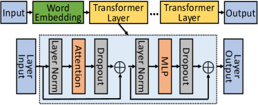
Figure 1: LLM architecture.

The attention layer in Fig. 1 includes the components below.

QKV generation. The attention layer takes a sequence embedding $E$ as an input. QKV generation conducts the following operations to generate $Q$, $K$, and $V$ of the sequence for head $h$:

$$Q^{h}=EW_{Q}^{h}\mbox{, \leavevmode\nobreak\ }K^{h}=EW_{K}^{h}\mbox{, \leavevmode\nobreak\ }V^{h}=EW_{V}^{h},\vspace{-0.1in}$$ (1)

where $W_{Q}^{h}$, $W_{K}^{h}$, and $W_{V}^{h}$ are the parameters for QKV generation in the attention head $h$. Table 1 lists the primary notations.

Self-attention. The self-attention layer takes $Q^{h}$, $K^{h}$, and $V^{h}$ as inputs, and outputs

$$O^{h}=\mbox{Softmax}(\frac{Q^{h}(K^{h})^{T}}{\sqrt{d_{h}}})V^{h}=P^{h}V^{h},\vspace{-0.1in}$$ (2)

where $P_{h}$ is the attention probability for head $h$. The softmax function operates row-wise on the input matrix $[a_{i,j}]$ as follows:

$$\frac{exp(a_{i,j})}{\sum_{k=1}^{t_{i}}exp(a_{i,k})},\vspace{-0.06in}$$ (3)

where $t_{i}$ is the index of the token on row $i$.

Post-self-attention linear. The post-self-attention linear layer takes $O^{h}$ from all heads as the input, and it outputs

$$O_{L}=[O^{1},O^{2},...,O^{N_{h}}]W_{L}=OW_{L},\vspace{-0.1in}$$ (4)

where $O$ is a concatenation of $O^{h}$, and $W_{L}$ is the parameter of the post-self-attention linear layer.

2.1 Chunked-Prefill

Chunked-prefill [18, 23] splits a long sequence into multiple sequence chunks, which are processed in different batches sequentially. In a batch, each chunk is coalesced with other decode tasks’ input tokens. Chunked-prefill alleviates the long generation stall caused by the interference between the prefill and decode stages, which occurs when a running request’s decode phase is interrupted by a new request’s prefill process, preventing the running decode from proceeding smoothly [18]. However, it cannot eliminate the generation-stall [24], especially when serving long prompts.

3 SP-based Prefilling

3.1 Experimental Analysis

We used 64 NVIDIA A100 GPUs, evenly distributed among 8 servers on 8 AWS p4d.24xlarge instances [25]. Each server has 96 vCPUs, 1152 GiB memory, and 400 Gbps bandwidth. Context window is the maximum sequence length under which a model is trained. Since most of the latest popular open-source models, such as Llama-3.1 [26] and Mixtral [27], do not support context lengths beyond 256K, we selected two well-known open-source models supported by vLLM [28] that offer a 1M context window – GLM-4-9B-Chat-1M [9] and InternLM2.5-7B-Chat-1M [10]. Table 2 lists the datasets we used. We ran Sarathi-Serve using TP=4 and PP=2 to guarantee that there was enough memory for serving prefill and decode requests with a 1M input length [10, 18]. The chunk size was set to 256 as Sarathi-Serve.

Dataset	Input Length			Output Length
	Median	P99	Std.	Median	P99	Std.
NeedleBench [29]	113K	995K	506K	348	572	174
BookCorpus [30]	97K	406K	183K	375	631	277

Table 2: NeedleBench has 11326 sequences, which are curated for evaluating the long-context models’ performance on the popular "needle-in-a-haystack" retrieval and reasoning tasks [31]. BookCorpus contains 7185 unique books with long and coherent texts for book summarization.

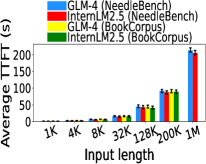
(a) Average TTFT.

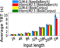
(b) Average TBT.

Figure 2: Average TTFT and TBT for different input lengths.

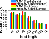
(a) Prefill throughput.

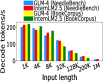
(b) Decode throughput.

Figure 3: Prefill and decode throughput of Sarathi-Serve.

Fig. 2 shows the average, the 1st and 99th percentiles of TTFT and TBT for requests in each input length group with different input lengths using NeedleBench and BookCorpus, respectively. Each $x$-axis index represents the group with input length within $(x-1,x]$. As the input length increases from 1K to 1M, TTFT increases from 1.6s to 213s, and TBT increases from 0.54s to 9.6s, demonstrating the inefficiency of sequential chunk processing. This dramatic increase results from the fact that the attention computation overhead scales quadratically with input length, and more chunks are constructed. Fig. 3 shows the prefill and decode throughput (tokens/s) of Sarathi-Serve. As the input length increases, the prefill and decode throughput decreases from 487 to 191 tokens/s and from 204 to 5 tokens/s.

O 1

Sequential processing of chunks of a long prompt generates long TTFT due to sequential chunk processing, high TBT from batching long-sequence prefills and decodes, and low throughput due to small batch size caused by constrained KV cache size and long sequences.

3.2 Design of SP-based Prefilling

3.2.1 SP-based Architectures

To address the issues highlighted in O 1 with handling long sequences in existing systems, we propose two SP architectures, as shown in Fig. 4 – one is for non-TP and one is for TP. Note this SP architecture is for one transformer layer and realizing PP is out of the scope of this paper. SP-NTP distributes QKV in heads across GPUs via the A2A communication for self-attention, and uses another A2A to distribute the self-attention output in Eq. (2) across GPUs. SP-TP lets each GPU (model partition) to process a SPT and uses all-gather to collect all partitions into each GPU for self-attention computation followed by the post-self-attention linear transformation in Eq. (4), and then uses reduce-scatter to combine and distribute the linear output.

Fig. 4(a) illustrates SP-NTP. Each GPU has a different SPT’s token embeddings (aka, hidden states) as the input to attention. Each GPU executes Eq. (1) for the first projection to calculate the QKV data of its SPT for all heads. Then, the heads are evenly split across GPUs for attention computation. For this purpose, the first A2A sends different head partitions’ QKV data from a GPU to their assigned GPUs. After the first A2A, each GPU has the QKV of the entire sequence for part of the heads, and then executes self-attention in Eq. (2). Next, it first gathers the head dimension and splits the sequence dimension of the self-attention output through the second A2A. Then, it conducts the second projection to get the final output via a linear matrix transformation as in Eq. (4).

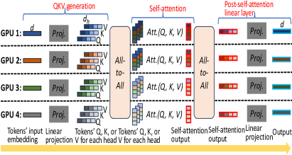
(a) SP-NTP for non-tensor parallelism.

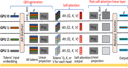
(b) SP-TP for tensor parallelism.

Figure 4: Two SP architectures for prefill.

Fig. 4(b) illustrates SP-TP. At the beginning, four GPU devices have their SPTs. Before the first linear projection, due to the use of TP, each GPU must collect all SPTs through all-gather. Then, each GPU executes the first projection (Eq. (1)) to obtain the QKV data of the entire sequence of its assigned heads since each GPU is responsible for certain heads (i.e., one head in this example) in TP. Then, each GPU conducts the attention computation on its QKV data (Eq. (2)) and outputs the self-attention result for that head partition. The second linear projection in the post-self-attention linear layer conducts a linear matrix transformation between the self-attention output $O^{h}$ and part $i$ of the parameters of the linear layer $W_{L}^{i}$, generating $O^{h}W_{L}^{i}$, a $L_{in}$-by-$d$ matrix. Next, using reduce-scatter, $O^{h}W_{L}^{i}$ from all GPUs are added together to obtain the $O_{L}$ in Eq. (4) and then split in sequence dimension into each GPU. In the example, each GPU outputs $O^{1}W_{L}^{1}$, $O^{2}W_{L}^{2}$, $O^{3}W_{L}^{3}$, and $O^{4}1W_{L}^{4}$, respectively. A reduce-scatter is conducted to achieve a reduce step $O_{L}=\sum_{i=1}^{4}O^{i}W_{L}^{i}$ and a scatter step that splits $O_{L}$ in the sequence dimension into each GPU.

One issue with SP is that the last SPT might not be the same length as other partitions, leading to low GPU utilization. To avoid this resource wastage, we insert the prefills of other shorter prompts to fully utilize KVC.

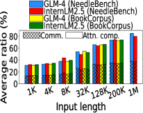
(a) SP-NTP.

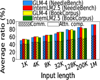
(b) SP-TP.

Figure 5: Ratios of communication and computation to TTFT.

3.2.2 How to Decide Between SP-NTP and SP-NT?

SP-NTP requires attention computation to use the complete model parameters of a layer. In TP, the parameters split across GPUs should be gathered into each GPU for attention computation at each layer, resulting in extra communication. For a long prompt, we determine the maximum SPT length that fully utilizes the KV cache, which dictates the number of GPUs used for prefill. Based on this GPU count, we select the SP architecture that minimizes communication overhead. This approach is explained in the supplementary material. Our experiments show that the length of a SPT can be 64K without TP and 128K for TP=8 in our experiment. Also, it is preferable to select SP-NTP to alleviate communication overhead if the input length is greater than 100K. The servers with the most available GPUs are chosen first in order to reduce the communication overhead.

3.2.3 Communication and Computation Overhead

SP-NTP involves two A2A communications, while SP-TP uses all-gather and reduce-scatter communications. We aim to measure the ratios of network communication time and attention computation time to TTFT, respectively. For SP-NTP, we set one SPT to 64K input tokens to fully utilize KV cache. For SP-TP, we set PP=1 and TP=8 such that it has enough GPU memory to serve a request with a 1M input length. We set one SPT to 128K input tokens to fully utilize KV cache. We put SPTs to GPUs within a node that has the maximum number of GPUs with available memory. If the number of GPUs is not enough, we select other nodes to place SPTs. Fig. 5 shows the two ratios in prefill with different input sequence lengths. We observe that SP-NTP generates 13-34% communication overhead and 18-43% attention computation overhead, and SP-TP generates 39-62% communication overhead and 11-29% attention computation overhead.

O 2

In the SP-based architectures, the network communication and attention computation may become bottlenecks.

3.2.4 Communication-Efficient Sparse Attention (CSA)

To address O 2, we propose communication-efficient sparse attention method (CSA). CRA reduces both communication and computation latency in SP-NTP, and computation latency in SP-TP. Since CSA does not reduce the communication overhead in SP-TP, we introduce a hierarchical communication method to address this issue. Below, we first explain how CSA operates in SP-NTP, followed by its operation in SP-TP.

CSA overview. Existing work has shown that tokens have a high correlation with other nearby tokens and a low correlation with far-away tokens in an extremely long sequence, thus dropping distant tokens during the attention computation of a token imposes little impact on the generation quality [19, 20]. Previous studies [32, 33, 34] identify token importance using attention scores and suggest dropping unimportant tokens to save KV cache. Based on these, to reduce communication overhead, CSA aligns GPU proximity with token proximity – closer SPTs are stored in nearer GPUs and vice versa, and drops more unimportant tokens among more distant ones and vice versa based on the accuracy decrease constraint specified by the user (which can be set to 0) in the first A2A communication. As a result, CSA transfers nearby tokens on high-speed paths, e.g., NVSwitch, and drops partial far-away tokens that need to pass low-speed paths to speed up A2A communication. Below, we outline the process for allocating SPTs to GPUs, determining the drop rate, and conducting communication and self-attention computation.

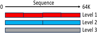
Figure 6: Processing SPTs in multiple levels.

Proximity-aware SPT allocation. For the purpose of only attending to the important far-away tokens, CSA treats a sequence in multiple levels as illutrated in Fig. 6. The sequence is partitioned into more segments at a lower level and vice versa, and the smallest segment is a SPT. To represent GPU distances when allocating SPTs, we assign each GPU a unique ID composed of three fields: RackID-ServerID-GPUID. For example, ID 0-11-010 represents GPU 2 in server 3 of rack 0. The difference between GPU IDs represents the distance between the GPUs. GPUs are sorted in the ascending order of their IDs. SPTs are sequentially placed on the sorted GPUs. As a result, closer partitions are mapped to closer GPUS.

Fig. 7 illustrates an example of CSA for a two-server case. Each server has two GPUs. Each GPU processes one SPT. All 4 SPTs are sequentially placed to GPU 1, 2, 3, and 4. Each GPU handles its segment in level-1. GPU 1-2 and GPU 3-4 handle the first and the second segment of level-2, respectively, marked by the red solid-line rectangle. GPU 1-4 handle the entire sequence of level-3, marked by the blue rectangle. In level-2, the first A2A collects nearby tokens from nearby GPUs in one segment via high-speed intra-server paths; in level-3, the first A2A collects far tokens from far GPUs in one segment, which involves inter-server paths. Each GPU computes the tokens’ self-attention output for each level and then uses the second A2A as shown in Fig. 4(a) to redistribute the self-attention output among GPUs for each level.

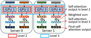
Figure 7: An example of CSA.

Level-based unimportant tokens dropping. A higher level handles a larger segment and drops more unimportant tokens so that a token attends to fewer distant tokens. The number of levels and the token drop ratio for each level are determined by a regression model (that will be introduced in § 3.2.6) based on the objectives of TTFT and accuracy degradation constraint. Suppose $p$ is the token drop ratio in level-2, for level $2+n$, we set its token drop ratio $p^{\prime}$ to a value that satisfies $1-p=(1-p^{\prime})/2^{n}$. This allows the number of tokens that a token attends to within a region (i.e., segment) to be roughly inversely proportional to the distance between the token and the attended region based on [19]. Attention score can represent a token’s importance. A problem here is how we can identify unimportant tokens before their attention scores are calculated. Existing work [34] indicates that except for the first and the last layer, the same head at close intermediate layers tends to have similar unimportant tokens. Therefore, a head at a layer uses the attention score from its previous layer to identify unimportant tokens. Specifically, the tokens are ordered based on their attention scores to be dropped. Note that 0 accuracy degradation constraint still enables dropping 22% of tokens and reduces 19% of communicaitont time and 28% computation time in our experiment (§ 5).

Communication and self-attention computation. Each segment at a level performs its attention computation, that is, a token attends to other remaining tokens in the same segment. As a result, a token attends to more nearby tokens located in smaller ranges, and fewer far-away tokens located in large ranges. Specifically, the SPTs (or their assigned GPUs) belonging to a segment at each level perform SP operation as in Fig. 4(a). However, rather than performing A2A communications in each segment at every level, CSA lets each GPU transmit all QKV data via the first A2A and transmit all self-attention output via the second A2A to each destination GPU only once.

For example, we have 4 GPUs for Fig. 6 and there are 4 attention heads (head 1-4). GPU1 and GPU2 handle the first segment in level-2, and they are assigned with heads 1-2 and heads 3-4, respectively. Similar to GPU 3 and GPU 4 in level-2. GPUs 1-4 handle the segment in level-3, and each GPU is assigned with one head in sequence. Fig. 8 gives two examples of QKV data transfer. Each rectangle in the figure represents Q, K, or V of a SPT for a head. GPU2 should send to GPU1 the QKV of remaining tokens in its SPT for head 1-2 at level-2 and for head 1 at level-3. Each GPU receives the determined dropping ratio for each level and drops the QKV values of unimportant tokens accordingly for QKV transmission. Since we keep the most important tokens in each level, the remaining tokens at level-2 include all remaining tokens at level-3. Therefore, GPU2 only needs to send the QKV data at level-2. In Fig. 8(b), GPU4 should send QKV of remaining tokens in its SPT to GPU3 for head 1-2 at level-2 and for head 3 at level-3. In this case, there is no duplicated data in the transmissions. Therefore, each GPU consolidates the QKV data across levels for each destination and sends it all at once. Each GPU conducts the self-attention for each level $i$ for its assigned head $h$, $O^{h}_{i}$. Then the second A2A is conducted within the segment. Then, each GPU receives its SPT’s $O_{i}^{h}$ of all heads for all levels, and it aggregates the data to calculate $O^{h}$ as below:

$$\vspace{-0.1in}\begin{split}O^{h}=\sum_{i=1}^{N_{v}}\frac{z^{h}_{i}}{\sum_{j}z^{h}_{j}}O^{h}_{i},\vspace{-0.2in}\end{split}\vspace{-0.3in}$$ (5)

where $N_{v}$ denotes the number of levels, $z^{h}_{i}$ denotes the denominator of the softmax in Eq. (3) for that token in level $i$ of head $h$, and $O^{h}_{i}$ is the attention output of that token in level $i$ of head $h$. Then, the GPU calculates the final self-attention output using Eq. (4). Dropped tokens are not involved in the communication and computation. However, the self-attention output of dropped tokens in each level is manually generated by filling with 0.

The communication overhead of the second A2A is also reduced. It redistributes less data along intra-server paths and more data along inter-server paths due to different token dropping ratios at different levels.

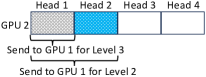
(a) GPU 2 sends data to GPU 1.

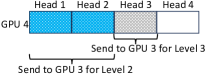
(b) GPU 4 sends data to GPU 3.

Figure 8: Two examples of QKV data to be transferred.

CSA in SP-TP and hierarchical communication. In SP-TP, since all tokens’ Q vectors need to participate in attention computation in each GPU, tokens cannot be dropped during the all-gather communication process. However, in the attention computation, CSA can be used to reduce the attention computation time due to fewer distant tokens.

We propose hierarchical communication for SP-TP’s all-gather and reduce-scatter to enhance communication-efficiency. For all-gather, each GPU sends the same token embedding data to every other GPU. To save the communication overhead, the GPU can transmit the data only once to the destination server, which broadcasts the data to its GPUs. Therefore, in this method, the GPUs within a server first collect their data into each GPU, and one GPU in each server sends its collected data to other servers. After a server receives the data, it broadcasts it to its GPUs. Reduce-scatter operates on the post-self-attention linear output across all GPUs. The communications between servers generates long latency. We leverage the post-self-attention linear outputs’ aggregation operation to reduce the transferred data volume across servers. Specifically, the GPUs within a server first reduce-scatter their own data, and then the servers reduce-scatter their reduced data. Note this method won’t be very effective for SP-NTP because its A2A communications do not have duplicated transferred data or data aggregation.

3.2.5 CSA-Enabled Pipelining

In CSA, QKV values from lower levels arrive earlier, with level-1 arriving first, followed by level-2, level-3, and so on. This allows the attention computation to begin as soon as the earlier QKV values arrive, enabling overlap between communication and computation. Below, we first present the pipelining for SP-NTP, followed by the pipelining for SP-TP.

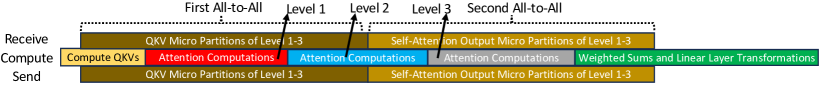
(a) SP-NTP.

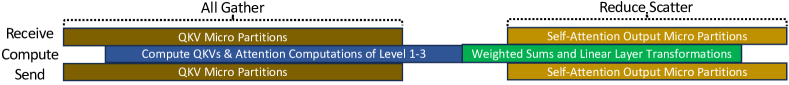
(b) SP-TP.

Figure 9: CSA-enabled communication-computation-communication three-phase pipelining.

How to split QKV tensors to enable pipelining? There are two options for partitioning QKV tensors: 1) in the head dimension, and 2) in the sequence dimension. Splitting heads is limited by the number of heads, which can range from 12 for small models to 96 for large ones [35]. It is hard to have a fine-grained partitioning plan with a small number of heads. Therefore, we choose to partition tensors in the sequence dimension. However, splitting QKV in the sequence dimension pauses the softmax computation until the entire softmax input $Q^{h}(K^{h})^{T}$ is obtained (Eq. (2)). Since softmax (Eq. (3)) is a row-wise operation, $Q^{h}$ can be split and parallelized, but $K^{h}$ should keep intact for each $Q^{h}$ partition. Therefore, softmax cannot start until the entire $K^{h}$ is received, which results in an inefficient pipeline. To solve the problem, we leverage online softmax [21] to conduct self-attention progressively using QKV partitions, as explained below.

Online softmax for QKV transmission pipelining. Online softmax computes the softmax (Eq. (3)) in an iterative manner. Instead of calculating the softmax for the entire $K^{h}$ and $V^{h}$ at once, it processes their partitions progressively. Online softmax allows Q tokens to be computed based on a partition of K and V (Eq. (2)) without waiting for other partitions of K and V to progressively compute $O^{h}$. It calculates and updates the denominator of softmax for each row every time Q is computed based on a KV partition, but it does not involve the denominator in the attention computation. After the attention computation between Q and all KV partitions (Eq. (2)) finishes, the denominator is eventually combined with the results to obtain the real self-attention output $O^{h}$. The stored denominator can be conveniently utilized for unimportant token identification. Online softmax introduces little overhead for storing the intermediate denominator, which is usually less than 0.1% of the QKV data. Let $S$ denote the number of input tokens, the data volume of QKV equals $3\times N_{h}\times S\times S$, while the denominator only accounts for $N_{h}\times S$. The denominator thus is only $\frac{1}{3\times S}$ of the QKV data, where $S$ is usually more than hundreds and thousands. The computational complexity remains the same as the original softmax.

CSA pipeline for SP-NTP. Fig. 9(a) presents an example of the pipelining in SP-NTP from the perspective of a GPU. We split the QKV data in sequence dimension for SP-NTP to overlap each of the two A2A communications with the computation. Since the QKV data at a lower level arrives earlier, the attention computation for all levels starts from a lower CSA level to a higher level. When the first micro QKV partition is computed through “Compute QKVs” as in Eq. (1), the GPU starts sending it to other GPUs and meanwhile receiving other GPUs’ micro QKV value partitions. After the GPU receives the QKV values of the first micro partition, it executes the attention computation to compute part of $O^{h}$ in Eq. (2). When this computation completes, the second A2A operation for this micro partition starts. But if this micro partition is not the first micro partition, the second A2A starts only after the second A2As of all preceding micro partitions at the same level have been completed. These steps repeat for the second and the third level. When the second A2A of this micro partition in all three levels completes, the weighted sum is calculated (Eq. (5)), and then the linear layer performs the linear transformation as in Eq. (4).

CSA pipeline for SP-TP. Fig. 9(b) presents an example of pipelining in SP-TP from the perspective of a GPU. SP-TP starts all-gather before the QKV computation and starts reduce-scatter after the post-self-attention linear transformation. Therefore, we split token embeddings in sequence dimension to overlap the all-gather and reduce-scatter communications with the computation. For SP-TP, its all-gather does not use CSA levels but its computation uses CSA levels. Then, each GPU sends the micro SPTs to nearby GPUs in priority so that GPUs can start the QKV and attention computation as soon as possible. As tokens are received from near to far on every GPU, a GPU can progressively conduct QKV generation in Eq. (1) and attention computation in Eq. (2) using micro SPTs for different levels. After the attention computations from all levels are completed for a micro partition, the weighted sum in Eq. (5) combines the self-attention outputs from all levels, and the linear layer performs the linear transformation as in Eq. (4), followed by reduce-scatter to overlap the computation and communication.

3.2.6 Objective-Oriented Configuring

This method determines the number of levels $N_{v}$ used by CSA, the number of micro partitions $M_{l,v}$ used for pipeline, and the token drop ratio $p_{l,h,v}$ for layer $l$, head $h$, and CSA level $v$ for two objectives. The first is how to minimize TTFT while adhering to the user-specified accuracy degradation $A_{d}=a_{c}-a^{\prime}_{c}$, where $a_{c}$ and $a^{\prime}_{c}$ are the inference accuracies without and with token dropping. The second is how to minimize $A_{d}$ while adhering to the user-specified TTFT.

Accuracy degradation constraint. Given input with length $L_{in}$, the factors influencing $A_{d}$ include the prompt length $L_{in}$, the number of levels $N_{v}$ used by CSA, and the token drop ratio $p_{l,h,v}$ for layer $l$, head $h$, and CSA level $v$. Therefore, we define the inference accuracy degradation function as $A_{d}=F_{A_{d}}(L_{in},N_{v},\{p_{l,h,v}\})$. Measuring $A_{d}$ for each combination of $(L_{in},N_{v},\{p_{l,h,v}\})$ is highly time-consuming, even when done offline. To approximate $F_{A_{d}}$, we build a regression model. In this work, to obtain the data used to train and test the regression model, we randomly separated $1/10$ sequences from NeedleBench, which will not be used in the experiment. For each selected sequence with input length $L_{in}$, we enumerated $N_{v}$ and $p_{l,h,v}$ to run each LLM to collect the data for training the regression model used to simulate $F_{A_{d}}$. We created 12564 samples, and split them into 4:1 for training and testing, respectively. The training process took 2 hours, and the trained regression model achieved 96% accuracy on the test set.

TTFT constraint. The factors influencing TTFT include $L_{in}$, $N_{v}$, $p_{l,h,v}$, network conditions, and the number of micro partitions, $M_{l,v}$, used by the pipeline at level $v$ and layer $l$. The TTFT for a prompt with $(L_{in},N_{v},\{p_{l,h,v}\},{M_{l,v}})$ is represented by TTFT $=T_{a}+T^{\prime}_{a}$, where $T_{a}$ is the attention computation time, and $T^{\prime}_{a}$ is the time not spent in the attention. $T^{\prime}_{a}$ depends on the prompt length $L_{in}$ and the GPU type ${G}$, and it scales proportionally with $L_{in}$ [23]. Therefore, it can be estimated using $T^{\prime}_{a}=RL_{in}$, where $R$ is the ratio to estimate $T^{\prime}_{a}$ and profiled offline. $T_{a}$ is expressed as:

$$T_{a}=\sum_{l=1}^{N_{l}}F_{pipe}(L_{in},N_{v},\{p_{l,h,v}\},\{M_{l,v}\},{G},{B}),$$ (6)

$$\mbox{ for }h=1,...,N_{h},\leavevmode\nobreak\ v=1,...,N_{v};$$

where ${B}$ is a matrix and denotes the available bandwidth between all pairs of GPUs. Due to pipelining complexity, accurately determining function $F_{pipe}$ is challenging. Thus, we use a simulator to simulate the pipelining to obtain $T_{a}$ with inputs:

$$\left(\mbox{ }\{T_{qkv}^{m_{1}}\},\{T_{1st\_a2a}^{m_{v},v}\},\{T_{attn}^{m_{v},v}\},\{T_{2nd\_a2a}^{m_{v},v}\},\{T_{linear}^{m_{1}}\}\mbox{ }\right),$$ (7)

$$\mbox{ for }m_{v}=1,...,M_{l,v};\leavevmode\nobreak\ v=1,...,N_{v}$$

where $T_{qkv}^{m_{1}}$ is the generation time of the $m_{1}$-th micro partition of QKV; $T_{1st\_a2a}^{m_{v},v}$, $T_{attn}^{m_{v},v}$, and $T_{2nd\_a2a}^{m_{v},v}$ are the first A2A transmission time, the attention computation time, and the second A2A communication time of the $m_{v}$-th micro partition at level $v$; $T_{linear}^{m_{1}}$ is the post-self-attention linear layer computation time of the $m_{1}$-th micro partition. $T_{qkv}^{m_{1}}$ is determined by ${G}$, $L_{in}$, and $M_{l,1}$. When level 1 finishes QKV generation, other levels can reuse the generated QKV. $T_{1st\_a2a}^{m_{v},v}$ and $T_{2nd\_a2a}^{m_{v},v}$ are determined by $p_{l,h,v}$, $L_{in}$, $m_{v}$ and the available bandwidth between GPU pairs involved at level $v$. $T_{attn}^{m_{v},v}$ is affected by $p_{l,h,v}$, $L_{in}$, $m_{v}$, and ${G}$. $T_{linear}^{m_{1}}$ is mainly determined by the matrix multiplication in which ${G}$, $L_{in}$, and $M_{l,1}$ are involved. Therefore, $T_{a}$ can be estimated and calculated offline for any combination of $(L_{in},N_{v},\{p_{l,h,v}\},\{M_{l,v}\},{G},{B})$.

Objectives and solutions. Let’s use $C_{TTFT}$ and $C_{A_{d}}$ to denote the constraint of TTFT and ${A_{d}}$, respectively. The first objective can be expressed by:

$$\underset{N_{v},\{p_{l,h,v}\},\{M_{l,v}\}}{\arg\min}({T_{a}}+T^{\prime}_{a}),$$ (8)

$$\mbox{ s.t. }F_{A_{d}}(S,N_{v},\{p_{l,h,v}\})\leq C_{A_{d}};$$

where $C_{A_{d}}$ is the constraint of $A_{d}$.

The second objective can be expressed by:

$$\underset{N_{v},\{p_{l,h,v}\},\{M_{l,v}\}}{\arg\min}F_{A_{d}}(S,N_{v},\{p_{l,h,v}\}),$$ (9)

$$\mbox{ s.t. }({T_{a}}+T^{\prime}_{a})\leq C_{TTFT};$$

We trained a regression model to output the best configuration of $N_{v}$, $\{p_{l,h,v}\}$, and $\{M_{l,v}\}$ with the inputs $C_{A_{d}}$, ${G}$, ${B}$, and $S$, which is used for online inference to solve the first objective function. The training data has 35289 samples, and the training took 5 hours. We also trained a regression model to output the best configuration of $N_{v}$, $\{p_{l,h,v}\}$, and $\{M_{l,v}\}$ with input $C_{TTFT}$, $C_{TBT}$, ${G}$, ${B}$, and $S$ to solve the second objective function. The training data has 29762 samples, and the training took 4 hours. We explain how we create the training data for training these regression models in the supplementary material.

4 SP-based decode

4.1 Experimental Analysis

Decode performance in SP. In this experiment, for each request, we chose the architecture between SP-NTP ad SP-TP with a shorter communication time judging by the input length as explained in LABEL:{sec:choose}. Fig. 11 shows the average, 1st, and 99th percentile TBT for each group of input lengths for NeedleBench and BookCorpus. Since BookCorpus does not have a sequence of 1M or more, only two bars are shown for NeedBench at the “1M” mark. TBT rises from 0.4s to 6.7s as the input length grows from 1K to 1M. Fig. 11 shows the decode throughput in tokens/s. As the sequence length increases from 1K to 1M, the decode throughput decreases from 357 to 5 decode tokens/s. For long prefill requests, as chunked-prefills continue, the KV data from previous chunks accumulates for attention calculations, increasing iteration latency. For a decode request with a long input length, its KV size is large. Since a single iteration mixes the prefill and decode requests, their large KV size increases both attention computation time and memory latency, leading to high TBT for decode tasks. Also, it leads to a small batch size and hence low decode throughput.

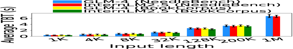
Figure 10: Average TBT.

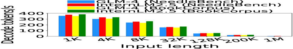
Figure 11: Decode throughput.

O 3

In the SP-based architectures, processing decodes along with the sequence partition prefills still leads to high TBT and low decode throughput.

Dataset (input length)	GLM-4		InternLM2.5
	Q	KV	Q	KV
NeedleBench (1M)	1ms	1173ms	1ms	1085ms
BookCorpus (406K)	1ms	984ms	1ms	879ms

Table 3: Latency of transferring Q and KV.

To address this issue, we propose SP-based decode method that decodes tokens separately from prefill and amortizes the KV cache overhead across GPUs. Coalescing a KV partition, rather than the entire KV data of a long sequence, with the KV data from shorter sequences allows more short sequences to be included in the decode batch, thereby forming a larger decode batch for a higher compute throughput. However, the GPU that admits the input token of the request needs to collect all missing KV data from other GPUs to complete the attention operation in Eq. (2), resulting in a long decode latency. The computation on all the KV values of previous tokens also take a long time. To minimize these latencies, instead of gathering KV values from all previous tokens, the GPU can broadcast the input token’s Q value to other GPUs, allowing them to compute attention with their respective KV partitions simultaneously, and then merge the outputs. Table 3 shows the latency of transferring Q and KV data in a model layer across 8 GPUs for two datasets with their maximum input length.

O 4

In the decode of a long sequence with distributed QKV values across GPUs, transferring the input token’s Q is much faster than transferring all KV partitions.

4.2 Design of SP-based Decode

After completing the prefill of a long-sequence request, we migrate the KV cache to other GPUs to process decode alongside non-long sequence tasks. We split its KV data into partitions to allow each partition to colocate with other requests’ KV data to increase throughput.

Fig. 12 gives an overview of how a long sequence decode is performed with other requests. Req1 is the long decode request (with a long KV), and Req2-5 are short decode requests (with a short KV). Req1’s KV is sharded across GPU 1 and GPU 2 for parallel computation. Req1’s input token is only fed to GPU 2, where its last KV partition is located. GPU1 handles the first half of Req1’s KV data and the entire KV data of Req2 and Req3, while GPU2 handles the second half of Req1’s KV data and the entire KV data of Req4 and Req5.

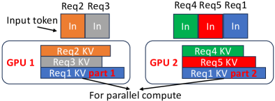
Figure 12: SP-based decode overview.

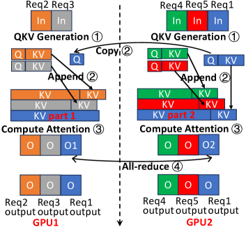
Figure 13: Process of SP-based decode.

Fig. 13 illustrates the process of the decode. Initially, GPU1 receives the input tokens from Req2 and Req3, and GPU2 receives the input tokens from both Req4, Req5, and Req1. In step ①, QKV generation is performed to compute the QKV values for the input tokens of all five requests. In step ②, all newly generated KV values are appended to each request’s respective KV cache and GPU2 broadcasts Req1’s Q values to the GPU1. Step ③ then uses the QKV values to perform attention computations as in Eq. (2): GPU1 computes the first part of Req1’s output (O1) and the complete output for Req2 and Req3, while GPU2 computes the second part of Req1’s output (O2) and the complete output for Req4 and Req5. Finally, in step ④, an all-reduce operation is performed to merge Req1’s outputs, O1 and O2. Note that the token dropping in prefill still can help reduce the computation overhead of decode.

5 Performance Evaluation

5.1 Implementation

Model implementation. We built our system on vLLM [28]. We extended the model code with our custom DistributedAttention class. We used the Triton [36] version of FlashAttention-2 [37] as the core attention but modified it to support CSA-enabled pipelining. We modified the LLMEngine and DistributedGPUExecutor in vLLM to enable SP and launch Ray [38] workers for SP partitions. The communication backend is NVIDIA Collective Communications Library (NCCL) [39].

SP communication. Each SPT on a GPU runs as a ray worker and communicates with each other via PyTorch’s distributed package with the NCCL backend.

Attention. The token-dropping determination and the weighted sum in Eq. (5) are implemented using Triton to minimize the time overhead. CSA is directly implemented in PyTorch to process tensors. The modified FlashAttention-2 can progressively process micro partitions in CSA pipeline.

5.2 Experiment Setup

We used the same experiment settings as in § 3.1. To limit the number of GPUs used, we did not employ PP. We set the default request arrival rate to 1 req/s, which was unlikely to increase the queueing delay, and used Poisson distribution to generate the request arrival times [28]. Based on the method introduced in § 3.2.2, we chose the number of GPUs, and either SP-NTP or SP-TP for a given request. Then, we determine its SPT length, which is 64K-128K in our experiment. We selected Sarathi-Serve as our baseline. We also included the Oracle, which uses the optimal hyper-parameters rather than relying on the regression models. Unless otherwise specified, CSPS has accuracy decrease constraint of 0 and may still have token dropping under the constraint. For one experiment, we also categorized the results for SP-NTP and SP-TP and presented them separately for reference.

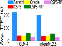
(a) NeedleBench.

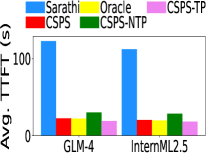
(b) BookCorpus.

Figure 14: Average TTFT.

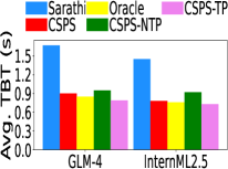
(a) NeedleBench.

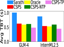
(b) BookCorpus.

Figure 15: Average TBT.

5.3 Overall Performance

Fig. 14 shows the average TTFT over requests. We see that Sarathi-Serve has 6.8-7.5$\times$ and 6.1-7.2$\times$ higher average TTFT compared to CSPS for NeedleBench and BookCorpus, respectively. The results indicate the effectiveness of CSPS’s CRA and pipelining methods in reducing TTFT. Fig. 15 shows the average TBT. We observe that Sarathi-Serve has 1.8-1.92$\times$ and 1.6-1.75$\times$ higher average TBT compared to CSPS for NeedleBench and BookCorpus, respectively. CSPS improves TBT owing to the dropping of KV data and the SP-based decode. CSPS has only 2-3% and 1-2% higher average TTFT than Oracle, and has only 3-4% and 2-4% higher average TBT than Oracle, showing the effectiveness of hyper-parameter configuring. CSPS-NTP has 1.35-1.48$\times$ and 1.32-1.51$\times$ higher average TTFT and 1.24-1.39$\times$ and 1.31-1.38$\times$ higher average TBT compared to CSPS-TP. This is because CSPS-NTP can process longer sequences more efficiently than CSPS-TP since A2A is proven to be more efficient than all-gather. CSPS-NTP is hence selected for longer sequences. From our experiment, we found that when CSPS has 0 accuracy degradation constraint, it still enables dropping 22% of tokens and reduces 19% of communication time and 28% computation time.

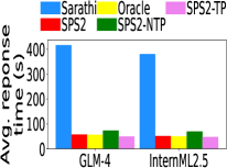
(a) NeedleBench.

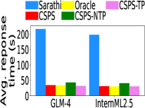
(b) BookCorpus.

Figure 16: Average response time.

Avg. throughput (tokens/s)	NeedleBench		BookCorpus
	GLM-4	InternLM2.5	GLM-4	InternLM2.5
Sarathi-Serve (prefill)	226	238	284	293
CSPS (prefill)	1580	1595	1615	1656
Oracle (prefill)	1595	1603	1620	1662
CSPS-NTP (prefill)	1615	1643	1648	1678
CSPS-TP (prefill)	1550	1567	1592	1612
Sarathi-Serve (decode)	5.2	8.2	9.3	9.6
CSPS (decode)	29	35	44	48
Oracle (decode)	32	37	48	51
CSPS-NTP (decode)	36	45	57	74
CSPS-TP (decode)	25	27	33	35

Table 4: Average throughput of prefill and decode.

Fig. 16 shows the average response time. We observe that Sarathi-Serve has 9.2-9.8$\times$ and 8.3-9.5$\times$ average response time compared to CSPS for NeedleBench and BookCorpus, respectively. CSPS improves response time because it has both more advanced SP-based prefill and decode. CSPS has only 2-3% and 2-4% higher average response time than Oracle, indicating the effectiveness of hyper-parameter configuring. CSPS-NTP has 1.35-1.47$\times$ and 1.34-1.43$\times$ average response time compared to CSPS-TP due to the aforementioned reason.

Table 4 shows the throughput in prefill and decode. CSPS increases the prefill throughput of Sarathi-Serve by 7.1-8.2$\times$ and increases its decode throughput by 4.3-5.2$\times$. Its throughput is only 2% lower than Oracle. CSPS-NTP produces 23-35% higher thoughput than CSPS-TP due to its higher capability of handling long prompts.

Fig. 17 shows the average response latency versus request rates. As the request rate climbs, the latency starts rising slowly but then abruptly spikes. This occurs when the request rate surpasses the serving system’s capacity, resulting in an unbounded increase in queue length and a consequent rise in latency for the requests. CSPS can deliver 1.6-2.5$\times$ higher request rate than Sarathi-Serve while sustaining the same latency. Sarathi-Serve combines prefill and decode in the same iteration, leading to longer iteration times. In contrast, CSPS separates and parallelizes prefill and decode while employing advanced methods for optimization.

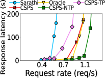
(a) GLM-4 (NeedleBench).

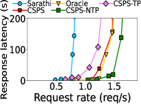
(b) GLM-4 (BookCorpus).

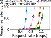
(c) InternLM2.5 (NeedleBench).

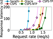
(d) InternLM2.5 (BookCorpus).

Figure 17: Average TBT vs. request rate.

6 Related Work

Recent efforts were made to efficiently serve LLMs. Orca [40] combines prompt processing and token generation in a batch for every iteration to fully utilize resources. vLLM [28] uses Paged Attention to enable a non-contiguous KV cache, which reduces memory fragmentation and increases throughput. HuggingFace TGI [41] and NVIDIA TensorRT-LLM [42] have also implemented the non-contiguous KV cache. Several other methods [43, 44, 24, 45] also achieve low-latency LLM serving such as splitting prefill and decode [24, 45]. AlpaServe [46] reduces the inference latency by determining an efficient strategy for splitting and placing a set of deep learning models [47]. FastGen [48] and Sarathi-Serve [18] chunk a long prompt and batch chunks sequentially with token generation tasks for inference tasks.

Sequence parallelism (SP) [49, 50, 51] was proposed for training. Other recent studies [52, 53, 54, 55, 56, 57, 58, 59, 60, 61, 62, 63, 19] proposed transformer variants to handle long sequences for training. However, LLM inference requires low latency, which has not been addressed in the previous work. This work is the first to propose SP infrastructure for LLM inference serving for long sequences that provides low latency.

7 Limitations and Future Work

CSPS separates prefill and decode, so when migrating KV data across nodes, if the bandwidth between nodes is limited, communication efficiency decreases. In the future, we plan to explore KV compression schemes for SP, which would not only accelerate SP-based prefill and reduce latency during KV migration under limited inter-node bandwidth but also reduce the size of the KV cache, alleviating GPU memory pressure to serve more long-sequence requests. Additionally, further GPU kernel optimizations can be applied to CSA and pipeline operations to reduce data transfers between GPU High-Bandwidth Memory (HBM) and registers, thereby increasing computational efficiency.

8 Conclusion

This paper presents CSPS, a sequence-parallelism based LLM serving system for long prompts. CSPS consists of two PS-based prefill architectures for non-TP and TP, and a SP-based decode architecture. It improves prefill by CSA, CSA-enabled pipelining, and objective-oriented configuring to determine the hyper-parameters used in the methods. Both real experiments and large-scale simulation show the superior performance of CSPS in comparison with the state-of-the-art.

Appendix A Considerations for Selecting SP Architectures.

When the attention is performed in a layer with TP, we can all-gather parameters needed for this layer into each GPU such that SP-NTP works in this case. In other words, SP-NTP is definitely used for model deployments without TP; for deployments with TP, SP-TP can be used, and SP-NTP can also be used as long as it all-gathers parameters into each GPU required by an attention operation. Whether SP-TP or SP-NTP is chosen for deployments with TP depends on how much data is transferred in each layer. The communication overhead for SP-NTP transferring parameters in each layer is $\frac{3d^{2}}{N}N(N-1)+\frac{d^{2}}{N}N(N-1)$, where $\frac{3d^{2}}{N}N(N-1)$ is from the parameter for QKV generation, and $\frac{d^{2}}{N}N(N-1)$ is from the parameter of the post-self-attention linear layer. The communication overhead of SP-NTP for two A2A communications is $\frac{3L_{in}d}{N^{2}}N(N-1)+\frac{L_{in}d}{N^{2}}N(N-1)$. The entire communication overhead of NTP-TP is $(4d^{2}+\frac{4L_{in}d}{N})(N-1)$. For SP-TP, it has one all-gather and one reduce-scatter. The communication overhead of them is $\frac{L_{in}d}{N}N(N-1)$ and $L_{in}d(1-\frac{1}{N})N$, respectively. The entire overhead of SP-NTP is $2L_{in}d(N-1)$. Therefore, when $(4d^{2}+\frac{4L_{in}d}{N})(N-1)<2L_{in}d(N-1)$, i.e., $\frac{d}{L_{in}}<\frac{1}{2}(1-\frac{2}{N})$, SP-NTP is better than SP-TP. Specifically, when $N=2$, SP-NTP is always better; when $N>2$, SP-NTP is better only if $L_{in}>2d\frac{N}{N-2}$. Since $d$ usually ranges from $\approx$ 4K (Llama-3.1 8B) to 16K (LLama-3.1 405B), SP-NTP is more suitable for deployments with TP when $L_{in}>2\times$16K$\frac{3}{3-2}=$96K.

Appendix B Train Regression Models for Hyper-Parameter Configuring

We enumerate $N_{v}$, $\{p_{l,h,v}\}$, and $\{M_{l,v}\}$ to obtain their corresponding TTFT and use $F_{A_{d}}$ to have their quality degradation ratio. For any enumeration that adheres to $C_{A_{d}}$, we select the one that has the least TTFT. However, there comes a problem of how to reduce the number of enumerations. The first factor to enumerate is the number of CSA levels $N_{v}$, which usually depends on the sequence length $S$. For a short sequence being able to be handled within a server, $N_{l}$ can be set to 1 (without CSA) or 2; for a sequence placed across servers but within a rack, $N_{v}$ can be 2 or 3; and for a sequence placed across racks, $N_{v}$ can be set to 3 or 4. The next factor to enumerate is all token drop ratios $\{p_{l,h,v}\}$ for each layer, each head, and each level. Level 1 always uses drop ratio $p_{l,h,1}=0$. For a head, since we have determined which layers have the same important and unimportant tokens offline, we allow those layers to have the same $p$ in the same level to reduce the number of enumerations. At CSA level 2 for a given head, since the trend of change in the standard deviation of attention scores in a layer roughly reflects the trend of change in $p$ that we should use, we only enumerate $p$ across layers according to the trend of change in the standard deviation of attention scores. For example, for layer $A$ and layer $B$ having the standard deviation $a$ and $b$, we enumerate $p$ in [$p^{a}-0.2,p^{a}+0.2$] in layer $A$ and enumerate $p$ in [$p^{b}-0.2,p^{b}+0.2$] in layer $B$, where $p^{a}:p^{b}=a:b$. The interval between two enumerations of $p$ is 0.02 to save time. When enumerating $p_{v_{2}}$ in CSA level 2, we set $p_{v_{2+n}}$ in level $2+n$ to a value that satisfies $1-p_{v_{2}}=(1-p_{v_{2+n}})/2^{n}$ for $n\geq 1$. This allows the number of tokens that a token attends to within a region to be roughly inversely proportional to the distance between the token and the attended region [19]. Hence, we only have to enumerate $p$ in level 2. The last one to enumerate is $\{M_{l,v}\}$. For CSA level 1, $M_{l,1}$ is the same for all layers because level 1 does not drop tokens and has the same data volume across layers. $M_{l,1}$ is enumerated between [4, 16] for communication and computation efficiency. At higher levels, $M_{l,v}$ is enumerated between smaller values [1, 8] or [1, 4] because higher levels have smaller data volumes and do not need too many micro partitions. Close layers also reuse $M_{l,v}$ to save time. If the enumeration for a factor breaks the constraint of $A_{d}$, it immediately stops to enumerate other factors. Through this method, we calculated the desired results offline for the given ${G}$, ${B}$, and $S$ to train the regression model.

We also trained a regression model to output the best configuration of $N_{v}$, $\{p_{l,h,v}\}$, and $\{M_{l,v}\}$ with input $C_{TTFT}$, ${G}$, ${B}$, and $S$ to solve the second objective function. The training data has 29762 samples, and the training took 4 hours. We enumerate all $N_{v}$, $\{p_{l,h,v}\}$, and $\{M_{l,v}\}$ that meet $C_{TTFT}$ and select the one that has the smallest $A_{d}$ to create the training data for the regression model.

References

- [1] Alec Radford, Jeffrey Wu, Rewon Child, David Luan, Dario Amodei, Ilya Sutskever, et al. Language models are unsupervised multitask learners. OpenAI blog, 1(8):9, 2019.
- [2] Tom Brown, Benjamin Mann, Nick Ryder, Melanie Subbiah, Jared D Kaplan, Prafulla Dhariwal, Arvind Neelakantan, Pranav Shyam, Girish Sastry, Amanda Askell, Sandhini Agarwal, Ariel Herbert-Voss, Gretchen Krueger, Tom Henighan, Rewon Child, Aditya Ramesh, Daniel Ziegler, Jeffrey Wu, Clemens Winter, Chris Hesse, Mark Chen, Eric Sigler, Mateusz Litwin, Scott Gray, Benjamin Chess, Jack Clark, Christopher Berner, Sam McCandlish, Alec Radford, Ilya Sutskever, and Dario Amodei. Language models are few-shot learners. In H. Larochelle, M. Ranzato, R. Hadsell, M.F. Balcan, and H. Lin, editors, Advances in Neural Information Processing Systems, volume 33, pages 1877–1901. Curran Associates, Inc., 2020.
- [3] Timo Schick, Jane Dwivedi-Yu, Roberto Dessi, Roberta Raileanu, Maria Lomeli, Luke Zettlemoyer, Nicola Cancedda, and Thomas Scialom. Toolformer: Language models can teach themselves to use tools. arXiv, 2023.
- [4] Facebook opt models. https://huggingface.co/models?sort=trending&search=facebook+opt, 2024.
- [5] Meta Llama-2. https://llama.meta.com/llama2/, 2024.
- [6] Meta Llama-3. https://llama.meta.com/llama3/, 2024.
- [7] Aydar Bulatov, Yuri Kuratov, and Mikhail S. Burtsev. Scaling transformer to 1m tokens and beyond with rmt. ArXiv, abs/2304.11062, 2023.
- [8] Hao Liu, Wilson Yan, Matei Zaharia, and Pieter Abbeel. World model on million-length video and language with blockwise ringattention. arXiv preprint arXiv:2402.08268, 2024.
- [9] GLM-4-9B-1M. https://huggingface.co/THUDM/glm-4-9b-chat-1m, 2024.
- [10] InternLM2.5-7B-Chat-1M. https://huggingface.co/internlm/internlm2_5-7b-chat-1m, 2024.
- [11] Gemini. https://gemini.google.com/, 2024.
- [12] Elozino Egonmwan and Yllias Chali. Transformer-based model for single documents neural summarization. In Proceedings of the 3rd Workshop on Neural Generation and Translation, pages 70–79, Hong Kong, November 2019. Association for Computational Linguistics.
- [13] Zi Gong, Cuiyun Gao, Yasheng Wang, Wenchao Gu, Yun Peng, and Zenglin Xu. Source code summarization with structural relative position guided transformer. In 2022 IEEE International Conference on Software Analysis, Evolution and Reengineering (SANER), pages 13–24, 2022.
- [14] Haopeng Zhang, Xiao Liu, and Jiawei Zhang. HEGEL: Hypergraph transformer for long document summarization. arXiv, 2022.
- [15] Ashutosh Adhikari, Achyudh Ram, Raphael Tang, and Jimmy Lin. Docbert: BERT for document classification. CoRR, abs/1904.08398, 2019.
- [16] Xiang Dai, Ilias Chalkidis, Sune Darkner, and Desmond Elliott. Revisiting transformer-based models for long document classification. arXiv, 2022.
- [17] GitHub Copilot. https://github.com/features/copilot/, 2024.
- [18] Amey Agrawal, Nitin Kedia, Ashish Panwar, Jayashree Mohan, Nipun Kwatra, Bhargav Gulavani, Alexey Tumanov, and Ramachandran Ramjee. Taming Throughput-Latency tradeoff in LLM inference with Sarathi-Serve. In 18th USENIX Symposium on Operating Systems Design and Implementation (OSDI 24), pages 117–134, Santa Clara, CA, July 2024. USENIX Association.
- [19] Jiayu Ding, Shuming Ma, Li Dong, Xingxing Zhang, Shaohan Huang, Wenhui Wang, Nanning Zheng, and Furu Wei. Longnet: Scaling transformers to 1,000,000,000 tokens. arXiv, 2023.
- [20] Mandy Guo, Joshua Ainslie, David Uthus, Santiago Ontanon, Jianmo Ni, Yun-Hsuan Sung, and Yinfei Yang. Longt5: Efficient text-to-text transformer for long sequences. arXiv preprint arXiv:2112.07916, 2021.
- [21] Maxim Milakov and Natalia Gimelshein. Online normalizer calculation for softmax. CoRR, abs/1805.02867, 2018.
- [22] SPS2 Code. https://anonymous.4open.science/r/SPS2.
- [23] Microsoft. DeepSpeed-FastGen: High-throughput Text Generation for LLMs via MII and DeepSpeed-Inference. https://github.com/microsoft/DeepSpeed/tree/master/blogs/deepspeed-fastgen.
- [24] Yinmin Zhong, Shengyu Liu, Junda Chen, Jianbo Hu, Yibo Zhu, Xuanzhe Liu, Xin Jin, and Hao Zhang. DistServe: Disaggregating prefill and decoding for goodput-optimized large language model serving. In 18th USENIX Symposium on Operating Systems Design and Implementation (OSDI 24), pages 193–210, Santa Clara, CA, July 2024. USENIX Association.
- [25] Amazon EC2 P4 instances. https://aws.amazon.com/ec2/instance-types/p4/.
- [26] Meta Llama-3.1. https://llama.meta.com/, 2024.
- [27] Mixtral. https://mistral.ai/technology/#models, 2024.
- [28] Woosuk Kwon, Zhuohan Li, Siyuan Zhuang, Ying Sheng, Lianmin Zheng, Cody Hao Yu, Joseph Gonzalez, Hao Zhang, and Ion Stoica. Efficient memory management for large language model serving with pagedattention. In Proceedings of the 29th Symposium on Operating Systems Principles, SOSP ’23, page 611–626, New York, NY, USA, 2023. Association for Computing Machinery.
- [29] Mo Li, Songyang Zhang, Yunxin Liu, and Kai Chen. Needlebench: Can llms do retrieval and reasoning in 1 million context window? arXiv preprint arXiv:2407.11963, 2024.
- [30] BookCorpus. https://huggingface.co/datasets/bookcorpus/bookcorpus, 2024.
- [31] Shouyuan Chen, Sherman Wong, Liangjian Chen, and Yuandong Tian. Extending context window of large language models via positional interpolation. arXiv preprint arXiv:2306.15595, 2023.
- [32] Zhenyu Zhang, Ying Sheng, Tianyi Zhou, Tianlong Chen, Lianmin Zheng, Ruisi Cai, Zhao Song, Yuandong Tian, Christopher Ré, Clark Barrett, Zhangyang "Atlas" Wang, and Beidi Chen. H2o: Heavy-hitter oracle for efficient generative inference of large language models. In A. Oh, T. Neumann, A. Globerson, K. Saenko, M. Hardt, and S. Levine, editors, Advances in Neural Information Processing Systems, volume 36, pages 34661–34710. Curran Associates, Inc., 2023.
- [33] Zichang Liu, Aditya Desai, Fangshuo Liao, Weitao Wang, Victor Xie, Zhaozhuo Xu, Anastasios Kyrillidis, and Anshumali Shrivastava. Scissorhands: Exploiting the persistence of importance hypothesis for llm kv cache compression at test time. In A. Oh, T. Neumann, A. Globerson, K. Saenko, M. Hardt, and S. Levine, editors, Advances in Neural Information Processing Systems, volume 36, pages 52342–52364. Curran Associates, Inc., 2023.
- [34] Suyu Ge, Yunan Zhang, Liyuan Liu, Minjia Zhang, Jiawei Han, and Jianfeng Gao. Model tells you what to discard: Adaptive kv cache compression for llms. arXiv preprint arXiv:2310.01801, 2023.
- [35] Megatron-LM and Megatron-Core. https://github.com/NVIDIA/Megatron-LM.
- [36] Triton. https://triton-lang.org/main/index.html#, 2024.
- [37] Tri Dao. Flashattention-2: Faster attention with better parallelism and work partitioning. arXiv preprint arXiv:2307.08691, 2023.
- [38] Ray. https://ray.io, 2024.
- [39] Nvidia collective communications library (NCCL). https://developer.nvidia.com/nccl.
- [40] Gyeong-In Yu, Joo Seong Jeong, Geon-Woo Kim, Soojeong Kim, and Byung-Gon Chun. Orca: A distributed serving system for Transformer-Based generative models. In 16th USENIX Symposium on Operating Systems Design and Implementation (OSDI 22), pages 521–538, Carlsbad, CA, July 2022. USENIX Association.
- [41] Hugging Face TGI. https://huggingface.co/text-generation-inference, 2024.
- [42] TensorRT-LLM. https://github.com/NVIDIA/TensorRT-LLM, 2024.
- [43] Wonbeom Lee, Jungi Lee, Junghwan Seo, and Jaewoong Sim. InfiniGen: Efficient generative inference of large language models with dynamic KV cache management. In 18th USENIX Symposium on Operating Systems Design and Implementation (OSDI 24), pages 155–172, Santa Clara, CA, July 2024. USENIX Association.
- [44] Biao Sun, Ziming Huang, Hanyu Zhao, Wencong Xiao, Xinyi Zhang, Yong Li, and Wei Lin. Llumnix: Dynamic scheduling for large language model serving. In 18th USENIX Symposium on Operating Systems Design and Implementation (OSDI 24), pages 173–191, Santa Clara, CA, July 2024. USENIX Association.
- [45] Pratyush Patel, Esha Choukse, Chaojie Zhang, Aashaka Shah, Íñigo Goiri, Saeed Maleki, and Ricardo Bianchini. Splitwise: Efficient generative llm inference using phase splitting. In 2024 ACM/IEEE 51st Annual International Symposium on Computer Architecture (ISCA), pages 118–132. IEEE, 2024.
- [46] Zhuohan Li, Lianmin Zheng, Yinmin Zhong, Vincent Liu, Ying Sheng, Xin Jin, Yanping Huang, Zhifeng Chen, Hao Zhang, Joseph E. Gonzalez, and Ion Stoica. AlpaServe: Statistical multiplexing with model parallelism for deep learning serving. In 17th USENIX Symposium on Operating Systems Design and Implementation (OSDI 23), pages 663–679, Boston, MA, July 2023. USENIX Association.
- [47] Lianmin Zheng, Zhuohan Li, Hao Zhang, Yonghao Zhuang, Zhifeng Chen, Yanping Huang, Yida Wang, Yuanzhong Xu, Danyang Zhuo, Eric P. Xing, Joseph E. Gonzalez, and Ion Stoica. Alpa: Automating inter- and Intra-Operator parallelism for distributed deep learning. In 16th USENIX Symposium on Operating Systems Design and Implementation (OSDI 22), pages 559–578, Carlsbad, CA, July 2022. USENIX Association.
- [48] Connor Holmes, Masahiro Tanaka, Michael Wyatt, Ammar Ahmad Awan, Jeff Rasley, Samyam Rajbhandari, Reza Yazdani Aminabadi, Heyang Qin, Arash Bakhtiari, Lev Kurilenko, and Yuxiong He. Deepspeed-fastgen: High-throughput text generation for llms via mii and deepspeed-inference. arXiv preprint arXiv:2401.08671, 2024.
- [49] Vijay Anand Korthikanti, Jared Casper, Sangkug Lym, Lawrence McAfee, Michael Andersch, Mohammad Shoeybi, and Bryan Catanzaro. Reducing activation recomputation in large transformer models. Proceedings of Machine Learning and Systems, 5:341–353, 2023.
- [50] Sam Ade Jacobs, Masahiro Tanaka, Chengming Zhang, Minjia Zhang, Shuaiwen Leon Song, Samyam Rajbhandari, and Yuxiong He. Deepspeed ulysses: System optimizations for enabling training of extreme long sequence transformer models. arXiv, 2023.
- [51] Shenggui Li, Fuzhao Xue, Yongbin Li, and Yang You. Sequence parallelism: Long sequence training from system perspective. CoRR, abs/2105.13120, 2021.
- [52] Sinong Wang, Belinda Z. Li, Madian Khabsa, Han Fang, and Hao Ma. Linformer: Self-attention with linear complexity. CoRR, abs/2006.04768, 2020.
- [53] Genta Indra Winata, Samuel Cahyawijaya, Zhaojiang Lin, Zihan Liu, and Pascale Fung. Lightweight and efficient end-to-end speech recognition using low-rank transformer. In ICASSP 2020 - 2020 IEEE International Conference on Acoustics, Speech and Signal Processing (ICASSP), pages 6144–6148, 2020.
- [54] Angelos Katharopoulos, Apoorv Vyas, Nikolaos Pappas, and François Fleuret. Transformers are rnns: Fast autoregressive transformers with linear attention. CoRR, abs/2006.16236, 2020.
- [55] Krzysztof Choromanski, Valerii Likhosherstov, David Dohan, Xingyou Song, Andreea Gane, Tamás Sarlós, Peter Hawkins, Jared Davis, Afroz Mohiuddin, Lukasz Kaiser, David Belanger, Lucy J. Colwell, and Adrian Weller. Rethinking attention with performers. CoRR, abs/2009.14794, 2020.
- [56] Zhen Qin, XiaoDong Han, Weixuan Sun, Dongxu Li, Lingpeng Kong, Nick Barnes, and Yiran Zhong. The devil in linear transformer. arXiv, 2022.
- [57] Juho Lee, Yoonho Lee, Jungtaek Kim, Adam Kosiorek, Seungjin Choi, and Yee Whye Teh. Set transformer: A framework for attention-based permutation-invariant neural networks. In Kamalika Chaudhuri and Ruslan Salakhutdinov, editors, Proceedings of the 36th International Conference on Machine Learning, volume 97 of Proceedings of Machine Learning Research, pages 3744–3753. PMLR, 09–15 Jun 2019.
- [58] Andrew Jaegle, Felix Gimeno, Andy Brock, Oriol Vinyals, Andrew Zisserman, and Joao Carreira. Perceiver: General perception with iterative attention. In Marina Meila and Tong Zhang, editors, Proceedings of the 38th International Conference on Machine Learning, volume 139 of Proceedings of Machine Learning Research, pages 4651–4664. PMLR, 18–24 Jul 2021.
- [59] Xuezhe Ma, Xiang Kong, Sinong Wang, Chunting Zhou, Jonathan May, Hao Ma, and Luke Zettlemoyer. Luna: Linear unified nested attention. In M. Ranzato, A. Beygelzimer, Y. Dauphin, P.S. Liang, and J. Wortman Vaughan, editors, Advances in Neural Information Processing Systems, volume 34, pages 2441–2453. Curran Associates, Inc., 2021.
- [60] Zihang Dai, Zhilin Yang, Yiming Yang, Jaime G. Carbonell, Quoc V. Le, and Ruslan Salakhutdinov. Transformer-xl: Attentive language models beyond a fixed-length context. CoRR, abs/1901.02860, 2019.
- [61] Aydar Bulatov, Yuri Kuratov, and Mikhail S. Burtsev. Scaling transformer to 1m tokens and beyond with rmt. arXiv, 2023.
- [62] Yuhuai Wu, Markus N. Rabe, DeLesley Hutchins, and Christian Szegedy. Memorizing transformers. arXiv, 2022.
- [63] Weizhi Wang, Li Dong, Hao Cheng, Xiaodong Liu, Xifeng Yan, Jianfeng Gao, and Furu Wei. Augmenting language models with long-term memory. arXiv, 2023.