Robust Federated Learning Over the Air: Combating Heavy-Tailed Noise with Median Anchored Clipping

Abstract

Leveraging over-the-air computations for model aggregation is an effective approach to cope with the communication bottleneck in federated edge learning. By exploiting the superposition properties of multi-access channels, this approach facilitates an integrated design of communication and computation, thereby enhancing system privacy while reducing implementation costs. However, the inherent electromagnetic interference in radio channels often exhibits heavy-tailed distributions, giving rise to exceptionally strong noise in globally aggregated gradients that can significantly deteriorate the training performance. To address this issue, we propose a novel gradient clipping method, termed Median Anchored Clipping (MAC), to combat the detrimental effects of heavy-tailed noise. We also derive analytical expressions for the convergence rate of model training with analog over-the-air federated learning under MAC, which quantitatively demonstrates the effect of MAC on training performance. Extensive experimental results show that the proposed MAC algorithm effectively mitigates the impact of heavy-tailed noise, hence substantially enhancing system robustness.

I Introduction

Federated learning (FL)[1, 2, 3, 4] is an emerging paradigm for collaborative data processing, enabling clients to benefit from high-quality model services while safeguarding the confidentiality of their private data. Nevertheless, significant challenges persist during the execution process. The frequent transmission of model information between clients and server consumes substantial network bandwidth, while the aggregation of a large number of parameters requires extensive computing resources. Moreover, although FL avoids directly aggregating user data, the exchange of model parameters could still pose risks to user privacy, particularly through inference attacks[5].

A viable solution to this problem is by integrating over-the-air (OTA) computation[6, 7, 8, 9] into the FL system, leveraging the superposition property of a multiple-access channel to automatically aggregate the clients’ gradient, significantly enhancing channel utilization while concurrently reducing computational overhead[10]. Furthermore, as the server receives aggregated gradients instead of individual ones from clients [11], the vulnerability to inference attacks is significantly reduced.

However, the analog channel inherently introduces electromagnetic interference during the transmission [12, 13, 14, 15]. While such interference enhances privacy protection, it also compromises the reliability of channel transmission, especially when it manifests as impulse interference, rendering the noise exhibiting a heavy-tailed distribution (rather than Gaussian) [16]—this has been consistently demonstrated by both theoretical[17] and empirical evidence [18]. In heavy-tailed distributions, extreme values (i.e., very large or very small values) occur with high probability, which could lead to severe signal distortion, resulting in a gradient explosion in the FL system and thereby profoundly affecting the training process of OTA FL.

Numerous methods have been proposed to combat the impact of strong channel noise, ranging from channel inversion[19], phase correction[20, 21], to amplitude correction and energy estimation[22]. However, these methods only enhance the channel quality and fail to cope with the heavy tail phenomenon at the algorithmic level. Gradient norm clipping (GNC) has been proposed for resolving gradient explosion problem[23], and has also been used for heavy-tailed gradient distribution problems[24], but there is a crucial limitation: Once the data statistical structure of the gradient is altered by noise, GNC struggles to maintain its effectiveness.

To enhance the robustness of OTA FL against heavy-tailed noise, we introduce a novel residual clipping technique named median anchored clipping (MAC). This method constrains the magnitude of signals received after centralization, adjusts the proportional relationships among gradients, maximizes gradient retention, and mitigates the impact of heavy-tailed interference on OTA FL. Our main contributions are summarized as follows:

• We propose a novel robust gradient clipping method tailored for OTA FL systems to mitigate the impact of heavy-tailed noise present in the analog channel.

• We derive the convergence rate of OTA FL gradient descent algorithm under MAC.

• We conduct substantial experiments where the results show that our MAC algorithm effectively mitigates the impact of heavy-tailed noise in analog OTA FL.

II System Model

II-A Setting

We consider the FL system depicted in Fig. 1, consisting of an edge server and $N$ clients. Every client $n$ possesses a local dataset $\mathcal{D}_{n}$ that contains $m_{n}$ data samples $\{(\boldsymbol{x}_{i},y_{i})\}^{m_{n}}_{i=1}$ where $\boldsymbol{x}_{i}\in\mathbb{R}^{d},y_{i}\in\mathbb{R}$. We assume the local datasets are statistically independent from each other. The edge server orchestrates with the clients to learn a statistical model from their datasets while preserving privacy.

More precisely, the clients need to collaboratively find a vector $\boldsymbol{w}\in\mathbb{R}^{d}$ that minimizes the following loss function:

$$f(\boldsymbol{w})=\frac{1}{N}\sum^{N}_{n=1}f_{n}(\boldsymbol{w})$$ (1)

where $f_{n}(\boldsymbol{w})$ is the local empirical risk of agent $n$. The solution of (1) is commonly known as the empirical risk minimizer, denoted by $\boldsymbol{w}^{*}=\arg\min f(\boldsymbol{w})$. And we adopt the OTA FL for model training in this paper.

II-B Federated Model Training Over the Air

The general procedure of analog OTA FL is detailed in [25]. We briefly describe it in this part for completeness. Particularly, at the $k$-th round of global communication, the edge server broadcasts the global parameter $\boldsymbol{w}_{k}$ to all the clients. Then, each client $n$ calculates its local gradient $\nabla f_{n}(\boldsymbol{w}_{k})$, modulates this parameter onto the magnitude of a set of common waveforms that are orthogonal to each other, and simultaneously sends the resulting analog signals to the edge server. The edge server passes the received signal to a bank of matched filters, with each branch tuned to one of the waveform bases, and outputs the automatically aggregated (but distorted) gradient. Formally, the global gradient can be written as follows:

$$\boldsymbol{g}_{k}=\frac{1}{N}\sum_{n=1}^{N}h_{n,k}\nabla f_{n}(\boldsymbol{w}_{k})+\boldsymbol{\xi}_{k}$$ (2)

in which $h_{n,k}$ represents the channel fading of client $n$ at the $k$-th global iteration, assumed to be a random variable with unit mean and finite variance, independent across the clients, and varies over time in an i.i.d. manner; $\boldsymbol{\xi}_{k}$ results from the electromagnetic interference, modeled as a $d$-dimensional random vector where each entry follows an independent symmetrical $\alpha$-stable distribution ($S\alpha S$)[26] (with tail index $\alpha$ and scale parameter $\tau$), accounting for the heavy-tailed distribution of impulse noise.

Consequently, the global parameter is updated as

$$\boldsymbol{w}_{k+1}=\boldsymbol{w}_{k}-\eta\boldsymbol{g}_{k},$$ (3)

where $\eta$ is the learning rate. Then the global parameter will be broadcasted to all clients for the next round of computations.

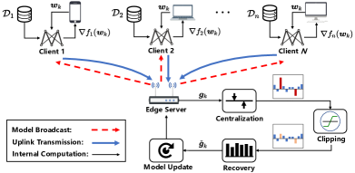
Figure 1: An illustration of the OTA FL training procedure.

II-C Unstable Training Performance

Normally, the above recursion is executed multiple rounds until convergence (if it occurs), upon which all participating entities have a common model close to $\boldsymbol{w}^{*}$. However, the spectrum is, by nature, a shared medium, giving rise to potentially strong co-channel interference, which typically manifests as noise during training. A notable feature of analog channel noise is its heavy-tail characteristic[18], which is manifested by frequent occurrence of impulse noise, which could lead to gradient explosion.

To that end, the main thrust of the present paper is to develop a scheme to cope with the noise introduced by analog OTA parameter aggregation so as to stabilize the training process and improve the performance of the trained model.

III Median Anchored Clipping

III-A Proposed Method

Our MAC algorithm strengthens the robustness of OTA FL against strong communication noise by performing three key steps for the aggregated gradients: 1) centralization, 2) clipping, and 3) recovery. The primary concept behind the MAC algorithm is to determine a datum point for a set of gradient entries and, anchoring on this point, recalibrate the magnitudes of entries.

To begin with, we define the vector-median as follows:

Definition 1

For a vector $\boldsymbol{w}\in\mathbb{R}^{d}$, med($\boldsymbol{w}$) is the median entry of all entries of $\boldsymbol{w}$, i.e., given $\boldsymbol{w}=(w_{1},w_{2},\dots,w_{d})^{T}$,

$$\texttt{med}(\boldsymbol{w})=\mathrm{median}\{w_{i},i\in[d]\}$$ (4)

where $[d]$ stands for the set $\{1,\dots,d\}$.

1) Centralization: Given a globally aggregated gradient $\boldsymbol{g}_{k}$, we centralize it by subtracting the vector-median from each entry, namely,

$$\boldsymbol{g}_{k}\leftarrow\boldsymbol{g}_{k}-\texttt{med}(\boldsymbol{g}_{k})\cdot\boldsymbol{1}$$ (5)

where $\boldsymbol{1}$ represents an all-ones vector.

The rationale behind centralizing the global gradient at the median is that this operation minimizes the L-1 deviation of the entries (note that due to heavy-tailed noise, the L-2 deviation of the entries may be unbounded). As such, during the subsequent clipping procedure, it preserves the original information of entries that are close to the median while eliminates the extreme values introduced by the impulse noise.

2) Clipping: Based on the centralized gradient $\boldsymbol{g}_{k}$, we perform value clipping to each entry, thereby constraining the range of individual entries within a specified threshold $C$. More concretely, for a generic entry $g_{k,i}$, $i\in[d]$, we have

$$g_{k,i}\leftarrow\texttt{sgn}(g_{k,i})\cdot\min(|g_{k,i}|,C)$$ (6)

where $\texttt{sgn}(\cdot)$ takes the sign of its input variable.

3) Recovery: After clipping the centralized gradient, we add back the median to each entry as follows:

$$\check{\boldsymbol{g}}_{k}\leftarrow\boldsymbol{g}_{k}+\texttt{med}(\boldsymbol{g}_{k})\cdot\boldsymbol{1}.$$ (7)

Toward this end, we obtain a new global gradient with the detrimental effects of heavy-tailed noise effectively alleviated while retaining the useful information as much as possible. The details of this method are summarized in Algorithm 1.

III-B Convergence Analysis

To facilitate the analysis, we make the following assumptions. , which are widely adopted in machine learning research.

Assumption 1

The objective function $f:\mathbb{R}^{d}\rightarrow\mathbb{R}$ is $\gamma$-strongly convex, i.e., for any $\boldsymbol{w},\boldsymbol{v}\in\mathbb{R}^{d}$, it is satisfied:

$$f(\boldsymbol{w})\geq f(\boldsymbol{v})+\langle\nabla f(\boldsymbol{v}),\boldsymbol{w}-\boldsymbol{v}\rangle+\frac{\gamma}{2}\|\boldsymbol{w}-\boldsymbol{v}\|^{2}.$$ (8)

Assumption 2

The objective function $f:\mathbb{R}^{d}\rightarrow\mathbb{R}$ is $L$-smooth, i.e., for any $\boldsymbol{w},\boldsymbol{v}\in\mathbb{R}^{d}$, it is satisfied:

$$f(\boldsymbol{w})\leq f(\boldsymbol{v})+\langle\nabla f(\boldsymbol{v}),\boldsymbol{w}-\boldsymbol{v}\rangle+\frac{L}{2}\|\boldsymbol{w}-\boldsymbol{v}\|^{2}.$$ (9)

Assumption 3

The gradients of each client are bounded, i.e., for $\forall n\in[N]$, there exists a constant $G$ that

$$\|\nabla f_{n}(\boldsymbol{w})\|\leq G.$$ (10)

At this stage, we are ready to present the main theoretical result of this paper as the following.

1 Initialize  $\boldsymbol{w}_{0}$

2for $k\in[K]$(communication round) do

3       for each client $n\in[N]$ in parallel do

4             Update local model: $\boldsymbol{w}_{k,n}=\boldsymbol{w}_{k}$.

5            Local training: $\nabla f_{n}(\boldsymbol{w}_{k})$.

6            Send $\nabla f_{n}(\boldsymbol{w}_{k})$ to the server.

7       end for

8      Global noisy aggregation:

9       $\boldsymbol{g}_{k}=\frac{1}{N}\sum_{n=1}^{N}h_{k,n}\nabla f_{n}(\boldsymbol{w}_{k})+\boldsymbol{\xi}_{k}$

10      Server receive $\boldsymbol{g}_{k}$:

11       $\check{\boldsymbol{g}}_{k}=$MAC$(\boldsymbol{g}_{k},C)$ // Median Anchored Clipping

12       $\boldsymbol{w}_{k+1}=\boldsymbol{w}_{k}-\eta\check{\boldsymbol{g}}_{k}$ // Server Update

13       Broadcasting $\boldsymbol{w}_{k+1}$ to clients.

14 end for

15

16 

17 Function $\mathbf{MAC}$($\boldsymbol{g},\mathit{C}$):

       Input: Gradient $\boldsymbol{g}$, threshold $C$

       Output: Clipped gradient $\boldsymbol{g}$

18       $\boldsymbol{m}=\text{med}(\boldsymbol{g})\times\boldsymbol{1}$

19      $\boldsymbol{g}=\boldsymbol{g}-\boldsymbol{m}$   // Centralization

20      for $g_{i}$ in $\boldsymbol{g}$ do

21             $g_{i}=\mathrm{sgn}(g_{i})\cdot\min\left\{|g_{i}|,C\right\}$  // Clipping

22       end for

23      

24      $\boldsymbol{g}=\boldsymbol{g}+\boldsymbol{m}$   // Recovery

25      return clipped gradient $\boldsymbol{g}$

26

27

Algorithm 1 OTA FL with MAC algorithm

Theorem 1

If the learning rate is set as $\eta\leq\frac{1}{L}$, then Algorithm 1 converges as

$$\mathbb{E}[\|\boldsymbol{w}_{k}\!-\!\boldsymbol{w}^{*}\|^{2} ]\!\leq\!\bigg{(}\!1-\eta\Big{(}\!\gamma p_{C}\!+\!\frac{\delta}{d}\left(1\!-\!p_{C}\right)\!\Big{)}\!\bigg{)}^{k}\!\|\boldsymbol{w}_{0}\!-\!\boldsymbol{w}^{*}\|^{2}$$

$$+\frac{\eta\left(d\left(C\!-\!2G\right)^{2}p_{C}+dC^{2}\left(1\!-\!p_{C}\right)\right)}{\gamma p_{C}+\frac{\delta}{d}\left(1\!-\!p_{C}\right)},$$ (11)

where $0<\delta<1$ and $p_{C}$ is

$$p_{C}=\mathbb{P}\{|\xi_{k,i}|\leq C-2G|\}\sim 1-\frac{\tau^{\alpha}}{C^{\alpha}}.$$ (12)

Proof:

We omit the proof due to space limitation. ∎

Remark 1

The result in (11) demonstrates that regardless of the heavy-tail index $\alpha$ and scale parameter $\tau$, running OTA FL in conjunction with MAC consistently achieves a linear convergence rate (where the residual error can be reduced by decreasing the learning rate). As such, the robustness of model training is substantially enhanced, making it resilient to the detrimental effects of heavy-tailed communication noise.

Remark 2

The effects of noise characteristics (including tail index and scale) and clipping threshold are quantified by $p_{C}$, which is determined within a probabilistic range. As (12) shows, these factors jointly influence the algorithm’s convergence rate.

IV Experimental Results

IV-A Experiment Setup

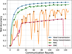
(a)

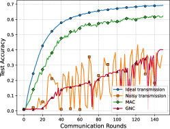
(b)

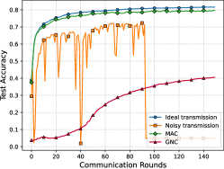
(c)

Figure 2: Performance comparison between MAC and the baselines, (a) training ResNet-18 on the CIFAR-10 dataset, (b) ResNet-34 on the CIFAR-100 dataset, and (c) training CNN on the FEMNIST dataset.

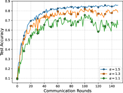
(a)

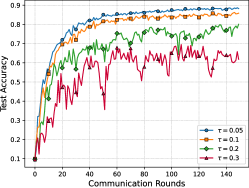
(b)

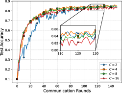
(c)

Figure 3: Sensitivity evaluation, (a)-(c) are training ResNet-18 on the CIFAR-10 dataset while non-i.i.d sampling, respectively correspond different heavy tail index $\alpha$, scale parameter $\tau$ and clipping threshold $C$.

System Setting: We examined the effectiveness of our proposed MAC algorithm by employing the GNC as a baseline and compared their training performances under the same configurations of OTA FL systems. In our experiment, Rayleigh fading with a parameter setting of $\mu=1$ is utilized for modeling channel fading. Unless otherwise stated, we set $N=50$, $\eta=0.03$, $E=5$, $\alpha=1.5$, $\tau=0.1$, and local batch size is 10.

Dataset and Models: We assessed performance on CIFAR-10, CIFAR-100[27], and FEMNIST (which is processed in a non-i.i.d manner)[28] using ResNet-18, ResNet-34[29], and CNN architectures, respectively. As the neural networks have a multi-layer structure, the MAC algorithm is executed parallel to the gradient blocks in a layer-wise manner. We also use a Dirichlet distribution with a concentration parameter of $Dir=0.3$[30, 31] to characterize data heterogeneity.

IV-B Performance Evaluation

In Fig. 2, we compare the performance of OTA FL under a variety of model training tasks, where the automatically aggregated but noisy global gradient undergoes MAC, GNC, and no post-processing (which we dub as noisy transmission), respectively. We also display the ideal scenario without any channel corruption (including fading and noise) as the performance upperbound. This figure shows that the training process is severely compromised by heavy-tailed noise, leading to fluctuations in the test accuracy curve and a marked decrease in the maximum accuracy achievable (by comparing the noisy transmission and ideal transmission). Under this circumstance, GNC encounters challenges in maintaining effective performance when the statistical structure of gradients, such as the proportional relationships among different gradient dimensions and the distribution of entries with varying magnitudes, is substantially disrupted by impulse noise. In contrast, the implementation of the MAC algorithm allows for a considerable reduction in these fluctuations, thereby significantly enhancing both test accuracy and training stability, robustfying the OTA FL system.

In Fig. 3, we examine the MAC performance by varying system-related parameters. Specifically, Fig. 3(a) and (b) compare the test accuracy of OTA FL MAC under different levels of communication noise. From Fig. 3(a), we can see that by decreasing the tail index from $\alpha=1.5$ to $\alpha=1.1$, the MAC algorithm exhibits consistent stability and achieves high test accuracy. Notably, the condition $\alpha=1.1$ represents a scenario with extreme volatility in the channel noise (where $\alpha=1$ corresponds to the Cauchy distribution characterized by undefined mean and variance), whilst MAC demonstrates remarkable robustness even under such extreme noise conditions. Fig. 3(b) examines the MAC performance in the presence of ascending scale parameter $\tau$. It is noteworthy that for $\tau=0.05$, $0.1$, $0.2$, and $0.3$, the SNR (defined as ratio between useful signal power and channel noise, i.e., SNR$=\|\nabla f(\boldsymbol{w}_{k})\|^{2}/\|\boldsymbol{\xi}_{k}\|^{2}$) are $-35$ dB, $-41$ dB, $-47$ dB, and $-50$ dB, respectively. The figure evidently confirms that our MAC algorithm exhibits substantial stability under challenging channel conditions, sustaining its performance even when the SNR reaches $-50$ dB. On the other hand, Fig. 3(c) presents a comparative analysis of the performance of the MAC algorithm across various clipping thresholds. The figure reveals that variations in threshold values result in similar convergence rates, indicating that the MAC algorithm is insensitive to the clipping thresholds, demonstrating the robustness and ease of parameterization inherent to the MAC algorithm.

V Conclusion

In this paper, we proposed a new algorithm, named MAC, which significantly enhances the robustness of OTA FL systems against channel noise that often exhibits heavy-tailed distributions. MAC leverages the median of the global gradient entries as a datum plane, and applies value clipping to truncate the extreme values induced by impulse noise, thereby effectively alleviating the detrimental effects of channel noise while largely preserving the original gradient information. We validated the effectiveness of MAC through convergence analysis and a set of empirical experiments, in which the MAC algorithm demonstrated consistent stability under various noise conditions. The MAC algorithm is effective, low-complex, and straightforward to be implemented, rendering it highly applicable in practical scenarios.

References

- [1] B. McMahan, E. Moore, D. Ramage, S. Hampson, and B. A. y Arcas, “Communication-efficient learning of deep networks from decentralized data,” in Proc. Int. Conf. Artif. Intell. Stat. (AISTATS), Fort Lauderdale, USA, Apr. 2017, pp. 1273–1282.
- [2] T. Li, A. K. Sahu, A. Talwalkar, and V. Smith, “Federated learning: Challenges, methods, and future directions,” IEEE Signal Process. Mag., vol. 37, pp. 50–60, May 2019.
- [3] J. Park, S. Samarakoon, M. Bennis, and M. Debbah, “Wireless network intelligence at the edge,” Proc. IEEE, vol. 107, no. 11, pp. 2204–2239, Oct. 2019.
- [4] Y.-J. Liu, S. Qin, Y. Sun, and G. Feng, “Resource consumption for supporting federated learning in wireless networks,” IEEE Trans. Wireless Commun., vol. 21, no. 11, pp. 9974–9989, June 2022.
- [5] L. Lyu, H. Yu, and Q. Yang, “Threats to federated learning: A survey,” Available as ArXiv:2003.02133, 2020.
- [6] B. Nazer and M. Gastpar, “Computation over multiple-access channels,” IEEE Trans. Inf. Theory, vol. 53, no. 10, pp. 3498–3516, Oct. 2007.
- [7] K. Yang, T. Jiang, Y. Shi, and Z. Ding, “Federated learning via over-the-air computation,” IEEE Trans. Wireless Commun., vol. 19, no. 3, pp. 2022–2035, Jan. 2020.
- [8] M. Frey, I. Bjelaković, and S. Stańczak, “Over-the-air computation in correlated channels,” IEEE Trans. Signal Process., vol. 69, pp. 5739–5755, Aug. 2021.
- [9] B. Xiao, X. Yu, W. Ni, X. Wang, and H. V. Poor, “Over-the-air federated learning: Status quo, open challenges, and future directions,” Fundam. res., Feb. 2024.
- [10] G. Zhu, J. Xu, K. Huang, and S. Cui, “Over-the-air computing for wireless data aggregation in massive iot,” IEEE Trans. Wireless Commun., vol. 28, no. 4, pp. 57–65, Sept. 2021.
- [11] A. Şahin and R. Yang, “A survey on over-the-air computation,” IEEE Commun. Surv. Tutor., Apr. 2023.
- [12] G. Zhu, Y. Wang, and K. Huang, “Broadband analog aggregation for low-latency federated edge learning,” IEEE Trans. Wireless Commun., vol. 19, no. 1, pp. 491–506, Oct. 2019.
- [13] M. M. Amiri and D. Gündüz, “Machine learning at the wireless edge: Distributed stochastic gradient descent over-the-air,” IEEE Trans. Signal Process., vol. 68, pp. 2155–2169, Mar. 2020.
- [14] H. Guo, A. Liu, and V. K. Lau, “Analog gradient aggregation for federated learning over wireless networks: Customized design and convergence analysis,” IEEE Internet Things J., vol. 8, no. 1, pp. 197–210, June 2020.
- [15] Z. Zhang, G. Zhu, R. Wang, V. K. Lau, and K. Huang, “Turning channel noise into an accelerator for over-the-air principal component analysis,” IEEE Trans. Wireless Commun., vol. 21, no. 10, pp. 7926–7941, Apr. 2022.
- [16] Z. Chen, H. H. Yang, and T. Q. Quek, “Edge intelligence over the air: Two faces of interference in federated learning,” IEEE Commun. Mag., Aug. 2023.
- [17] D. Middleton, “Statistical-physical models of electromagnetic interference,” IEEE Trans. Electromagn. Compat., no. 3, pp. 106–127, Aug. 1977.
- [18] L. Clavier, T. Pedersen, I. Larrad, M. Lauridsen, and M. Egan, “Experimental evidence for heavy tailed interference in the iot,” IEEE Commun. Lett., vol. 25, no. 3, pp. 692–695, Oct. 2020.
- [19] N. Mital and D. Gündüz, “Bandwidth expansion for over-the-air computation with one-sided csi,” in Proc. IEEE Int. Symp. on Inf. Theory (ISIT), Espoo, Finland, June 2022, pp. 1271–1276.
- [20] T. Sery and K. Cohen, “On analog gradient descent learning over multiple access fading channels,” IEEE Trans. Signal Process., vol. 68, pp. 2897–2911, Apr. 2020.
- [21] J. Lee, Y. Jang, H. Kim, S.-L. Kim, and S.-W. Ko, “Over-the-air consensus for distributed vehicle platooning control (extended version),” Available as ArXiv:2211.06225, 2022.
- [22] M. Goldenbaum and S. Stańczak, “Computing the geometric mean over multiple-access channels: Error analysis and comparisons,” in Asilomar Conf. on Signals, Systems. and Computers. (ACSSC), Pacific Grove, CA, USA, Nov. 2010, pp. 2172–2178.
- [23] R. Pascanu, T. Mikolov, and Y. Bengio, “On the difficulty of training recurrent neural networks,” in Proc. Int. Conf. Mach. Learn. (ICML), Atlanta GA USA, June 2013, pp. 1310–1318.
- [24] H. Yang, P. Qiu, and J. Liu, “Taming fat-tailed (“heavier-tailed” with potentially infinite variance) noise in federated learning,” vol. 35, New Orleans, Louisiana, USA, Nov. 2022, pp. 17 017–17 029.
- [25] H. H. Yang, Z. Chen, T. Q. Quek, and H. V. Poor, “Revisiting analog over-the-air machine learning: The blessing and curse of interference,” IEEE J. Sel. Topics Signal Process., vol. 16, no. 3, pp. 406–419, Dec. 2021.
- [26] G. Samorodnitsky, M. S. Taqqu, and R. Linde, “Stable non-gaussian random processes: stochastic models with infinite variance,” Bull. London Math. Soc, vol. 28, no. 134, pp. 554–555, 1996.
- [27] A. Krizhevsky, “Learning multiple layers of features from tiny images,” Master’s thesis, University of Tront, 2009.
- [28] S. Caldas, S. M. K. Duddu, P. Wu, T. Li, J. Konečnỳ, H. B. McMahan, V. Smith, and A. Talwalkar, “Leaf: A benchmark for federated settings,” Available as ArXiv:1812.01097, 2018.
- [29] K. He, X. Zhang, S. Ren, and J. Sun, “Deep residual learning for image recognition,” in Proc. IEEE Comput. Soc. Conf. Comput. Vis. Pattern Recognit. (CVPR), Las Vegas, NV, USA, June 2016, pp. 770–778.
- [30] D. A. E. Acar, Y. Zhao, R. M. Navarro, M. Mattina, P. N. Whatmough, and V. Saligrama, “Federated learning based on dynamic regularization,” Available as ArXiv:2111.04263, 2021.
- [31] T.-M. H. Hsu, H. Qi, and M. Brown, “Measuring the effects of non-identical data distribution for federated visual classification,” Available as ArXiv:1909.06335, 2019.