Combustion Toolbox: An open-source thermochemical code for gas- and condensed-phase problems involving chemical equilibrium
Abstract
The Combustion Toolbox (CT) is a newly developed open-source thermochemical code designed to solve problems involving chemical equilibrium for both gas- and condensed-phase species. The kernel of the code is based on the theoretical framework set forth by NASA’s computer program CEA (Chemical Equilibrium with Applications) while incorporating new algorithms that significantly improve both convergence rate and robustness. The thermochemical properties are computed under the ideal gas approximation using an up-to-date version of NASA’s 9-coefficient polynomial fits. These fits use the Third Millennium database, which includes the available values from Active Thermochemical Tables. Combustion Toolbox is programmed in MATLAB with an object-oriented architecture composed of three main modules: CT-EQUIL, CT-SD, and CT-ROCKET. The kernel module, CT-EQUIL, minimizes the Gibbs/Helmholtz free energy of the system using the technique of Lagrange multipliers combined with a multidimensional Newton-Raphson method, upon the condition that two state functions are used to define the mixture properties (e.g., enthalpy and pressure). CT-SD solves processes involving strong changes in dynamic pressure, such as steady shock and detonation waves under normal and oblique incidence angles. Finally, CT-ROCKET estimates rocket engine performance under highly idealized conditions. The new tool is equipped with a versatile Graphical User Interface and has been successfully used for teaching and research activities over the last four years. Results are in excellent agreement with CEA, Cantera within Caltech’s Shock and Detonation Toolbox (SD-Toolbox), and the Thermochemical Equilibrium Abundances (TEA) code. CT is available under an open-source GPLv3 license via GitHub https://github.com/CombustionToolbox/combustion_toolbox, and its documentation can be found in https://combustion-toolbox-website.readthedocs.io.
keywords:
Thermochemistry , shock wave , detonation , oblique front , rocket performance , GUI1 Introduction
The computation of chemical equilibrium has been widely used during the last century to determine the composition of multi-component mixtures subject to complex thermochemical transformations. The resulting mathematical problem is simple in systems involving only a few species, such as the complete combustion of rich hydrocarbon-air mixtures, or the dissociation of diatomic gas mixtures, e.g., air at moderate temperatures. However, the incomplete combustion of a typical hydrocarbon, for instance, methane, with air, involves hundreds of reactions and more than fifty species [1], which makes finding the final equilibrium state of the products a challenging task.
Two equivalent methods can be employed to determine the composition of the products at equilibrium: using equilibrium constants or minimizing the Gibbs/Helmholtz free energy of the system [2]. The first method requires specifying a sufficiently large set of elementary reactions at equilibrium (see, e.g., Refs. [3, 4, 5, 6, 7, 8, 9]). This favors the second, where each species is treated independently, and the focus is shifted to the chemical potentials of the different species involved [10, 11]. The second method was first introduced by the pioneering work of White in 1958 [12] and has become the cornerstone in the development of virtually all state-of-the-art thermochemical codes [13, 14, 15, 16, 17, 18, 19, 20, 21, 22, 23, 24, 25, 26, 27, 28, 29, 30].
The solution to the resulting minimization problem requires the evaluation of the thermodynamic properties of all species involved at a given temperature. For this purpose, extensive thermodynamic databases have been compiled, such as the NIST-JANAF tables [31, 32], NASA’s polynomials [33] and, more recently, the Third Millennium (Burcat) Database [34] with updates from Active Thermochemical Tables (ATcT) [35] to evaluate the enthalpies of formation. The ATcT rely on the use of a complete thermochemical network (TN) instead of the more traditional datasets based on individual reactions. The use of the full TN yields more accurate results that are, in addition, fully documented (uncertainties included). But more important is the fact that databases are easily updated with new knowledge, and readily provide new values for the thermochemical properties of all species [36].
A recent work by Scoggins et al. [37] reported an exhaustive review of over 1200 unique chemical species from several databases that fully (Goldsmith [38] and Blanquart [39, 40, 41, 42]), partially (Burcat), or did not (NASA) rely on the ATcT. They identified significant differences between Burcat’s and NASA’s databases due to the inconsistency of the species enthalpy of formation in the latter. Although this type of analysis is out of the scope of this work, all chemical species from Burcat’s database are also available in Combustion Toolbox (CT) and can be identified by the suffix “_M”. Thus, when both databases contain a given species, the final choice is left to the user.
Thermochemistry is firmly rooted in the study of combustion problems, high-speed flows, reactive and non-reactive shocks, rocket engine performance, and high explosives [43, 44]. For instance, strong hypersonic shocks involve changes in the molecular structure of the gas, including vibrational excitation leading to dissociation [45, 46], and later electronic excitation leading to ionization [47], which eventually transform the gas into a plasma. Turbulent combustion and gaseous detonations have also been the topic of intense research due to their high thermodynamic efficiency in propulsion applications [48, 49]. But they often exhibit strong deviations from equilibrium due to the wide range of length and time scales involved, making it necessary to rely on complex fluid dynamical analyses and numerical simulations with a high computational cost [50, 51]. Despite the deep understanding provided by the latter approach, there are still cases in which a proper physical explanation can not be found based only on numerical results. In these cases, separation of scales may allow to split the problem into simpler ones, where the assumption of chemical equilibrium could be justified in some representative scenarios [52, 45, 53].
Chemical equilibrium can be formulated either for single-phase gas mixtures [12, 21, 22, 19, 25, 26, 7, 8], single-phase gas mixtures with pure-condensed species—as in NASA’s CEA code [17], Refs. [3, 14, 6], and this work [30]—or for multi-phase systems [15, 16, 54, 18, 20, 23, 4, 24, 5, 27, 28, 55, 29, 9]. The latter case requires special treatments to ensure that the global minimum is reached, due to the non-convexity of the Gibbs free energy [20, 23, 56]. These include global optimization methods like the tunneling method [57] or differential evolution [58, 59].
The above review has identified many thermochemical codes currently available to the community. Nevertheless, to the best of our knowledge, there is not yet an open-source code based on up-to-date databases, written in a high-level programming language, fully documented, with high-performance computing capabilities, able to model a wide variety of applications, and equipped with a user-friendly Graphic User Interface (GUI). Combustion Toolbox was conceived with these long-term goals in mind, and is now presented and validated in this work. This MATLAB-GUI thermochemical code represents the core of an ongoing research work and has been used to investigate a series of problems during the last few years [52, 45, 60, 53, 61, 62, 63, 64, 65]. Results are in excellent agreement with NASA’s CEA code [17], Cantera [66] within Caltech’s Shock and Detonation Toolbox (SD-Toolbox) [67, 68], and the Thermochemical Equilibrium Abundances (TEA) code [25].
The paper is structured as follows. Section 2 starts with an initial overview of CT. The equilibrium kernel (CT-EQUIL) is presented in Section 3. The shock and detonation module (CT-SD) is discussed in Section 4, followed by the rocket performance module (CT-ROCKET) in Section 5. The results of all modules are validated against other codes in Sections 3 to 5. A detailed description of the GUI is given in Section 6. And, finally, the conclusions are presented in Section 7.
2 Overview of Combustion Toolbox
Combustion Toolbox [30] is a GUI-based thermochemical code written in MATLAB with an equilibrium kernel based on the mathematical formulation set forth by NASA’s CEA code [17]. The thermodynamic properties of the gaseous species are modeled with the ideal gas equation of state (EoS), and an up-to-date version of NASA’s 9-coefficient polynomial fits (NASA9) based on [33, 34, 35]. CT is a new thermochemical code written from scratch in a object-oriented architectural format composed of three main modules: CT-EQUIL, CT-SD, and CT-ROCKET.
The kernel module, CT-EQUIL, computes the composition at the equilibrium of multi-component gas mixtures that undergo canonical thermochemical transformations from an initial state (reactants), defined by its initial composition, temperature, and pressure, to a final state (products), defined by a set of chemical species (in gaseous—included ions—or pure condensed phase) and two thermodynamic state functions, such as enthalpy and pressure, e.g., for isobaric combustion processes. CT-SD solves steady-state shock and detonation waves in either normal or oblique incidence. Finally, CT-ROCKET computes the theoretical performance of rocket engines under highly idealized conditions. Even though all modules are enclosed in a user-friendly GUI, they can also be accessed from MATLAB’s command line in plain code mode.
There is a fourth closed-source (i.e., proprietary) module, CT-EXPLO, that estimates the theoretical properties of high explosive mixtures and multi-component propellants with non-ideal EoS. Although still under development, CT-EXPLO is distributed in its current form as the thermochemical module of SimEx [60] subject to a proprietary license. Further details on this module will be provided elsewhere.
2.1 Software Architecture
As previously mentioned, the program was developed from scratch using MATLAB and an object-oriented architectural design. All the modules rely on CT-EQUIL to compute the thermodynamic properties of the species involved and the chemical composition of the mixtures at equilibrium. The full package can be accessed from the GUI (see Section 6) or directly from MATLAB’s command line. Additionally, the main computations performed using the GUI are callbacks to the plain code. Consequently, any change made to the code is immediately reflected in the GUI, leading to a more flexible and adaptable tool.
MATLAB was selected as programming language due to its excellent linear algebra, visualizing and debugging capabilities, extensive documentation, active community, and dedicated app development framework (App Designer). CT has significantly evolved since its version 1.0.5 [69, 61], which relied solely on procedural techniques for performance advantages over MATLAB Object-Oriented Programming (OOP). However, the current version, v1.1.0 [30], has been completely rewritten using the OOP paradigm due to the inherent limitations of procedural techniques, such as reduced code modularity and scalability. After meticulous optimization, the new object-oriented-based code has achieved substantial performance improvements, achieving between and better performance compared to the previous version under identical test conditions. Even though MATLAB is an interpreted language, which introduces a significant performance cost compared to other (compiled) languages [70], CT computational times are still competitive compared to similar codes. For instance, as shown in Section 4, CT is about one order of magnitude faster than the MATLAB version of Caltech’s SD-Toolbox used with Cantera (written in C++). However, there is room for further improvement by isolating specific demanding tasks into C++ subroutines and accessing them from MATLAB using MEX files. Moreover, the adoption of OOP in the current version facilitates the parallelization of the code. These optimization techniques will be explored in future code releases.
The classes and methods included in CT’s modules (described in detail later) rely on several core and database classes. The most relevant among these are:
-
1.
Species: stores the properties and thermodynamic functions of a chemical species.
-
2.
ChemicalSystem: encapsulates the chemical species and phases within a chemical system.
-
3.
Mixture: represents a multi-component mixture, including its thermodynamic properties and the solution of the problem at hand.
-
4.
EquationState: defines the thermodynamic equation of state for a Mixture.
-
5.
Database: an abstract superclass with common methods and properties for database-related classes.
- 6.
For efficient data access, the Species class employs griddedInterpolant objects (see MATLAB’s built-in function griddedInterpolant.m), which use piecewise cubic Hermite interpolating polynomials (PCHIP) [71]. This approach speeds up the thermodynamic data access by a factor of 200% with respect to the evaluation of NASA’s polynomials. Starting from v1.1.0, these objects are also temporally allocated in cache for even better performance. Furthermore, for temperatures outside the bounds, we avoid the higher order terms of the polynomials by linear extrapolation, similar to Ref. [7], extending the range of validity of the thermodynamic data available. It should be emphasized that this extension is limited to a narrow temperature range and may not apply to temperatures significantly outside the bounds.
The Combustion Toolbox is organized using namespaces. Hence, it is necessary to import the different subpackages into MATLAB workspace as follows
The first statement imports a specific class or method, while the second imports an entire subpackage. To start working with CT, we also need to load/generate a database and initialize the chemical system. This can be easily done with one of the following sample statements:
In these examples, DB represents an instance of the database class used, e.g., DB = NasaDatabase(). The first option initializes the system with all the possible species that could arise based on the elements present in the reactants (see class’s method findProducts). The second option initializes the system with an extended list of 94 species that typically appear in CHON mixtures, including solid carbon C(gr). Finally, the third option restricts the system to a specific list of species that may appear as products.
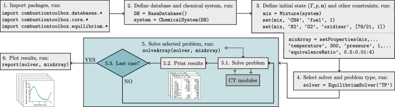
Figure 1 summarizes the main steps required to solve a problem with CT. First, import the necessary packages. Second, define the database and initialize the chemical system using one of the statements indicated above. Then, specify the initial state of the mixture (temperature, pressure, and molar composition), select the solver, and define the problem type. Depending on the problem’s constraints, additional parameters may be required, e.g., for planar shocks, it is necessary to specify the pre-shock velocity in m/s or, equivalently, the pre-shock Mach number. Once the setup is complete, invoke the solveArray method from the selected solver to compute the results. Finally, for post-processing, CT solvers include a built-in report method that shows predefined plots. Results can be exported using the Export class, which allows to save data into a spreadsheet or as a .mat file.
The CT source code is organized into several top-layer folders: +combustiontoolbox, databases, examples, gui, installer, modules, utils, and validations. The +combustiontoolbox folder encapsulates the different modules (namespaces) implemented in CT, such as CT-EQUIL (+equilibrium), CT-SD (+shockdetonation), and CT-ROCKET (+rocket). The databases folder mainly consists of raw data and .mat files that contain the thermochemical properties of the individual chemical species [33, 34, 35]. The examples folder includes various examples that demonstrate the wide variety of problems that can be solved with CT. The gui folder contains the routines that are specifically designed for the GUI. The installer folder contains all the installation files of the GUI: the MATLAB toolbox and the royalty-free stand-alone versions for different operative systems. This step is straightforward (see INSTALL.m), and further details can be found on the CT website (https://combustion-toolbox-website.readthedocs.io/en/latest/install.html). Finally, the validation folder includes the routines used to validate CT with the results obtained with other codes, the unit testing files to ensure the correct functionality of the code, and all the graphs generated from these verifications.
2.2 Collaborative framework and version control system
The collaborative process of open-source code can greatly benefit from the contributions of other authors. However, in the absence of adequate tools, this process may become disorderly. To mitigate this risk, we employ Git as version control system (VCS) and GitHub as online hosting service. These technologies enable comprehensive tracking of all changes made to the code while maintaining complete transparency throughout the development process [72, 73, 74, 75]. To further ensure the integrity of the package, all contributions are subject to rigorous testing before being merged into the two primary branches (master and develop) using GitHub Actions, providing a powerful tool to retrace errors in the code.
2.3 Documentation
A notable fraction of open-source codes lack sufficient documentation, which impedes the code’s usability and accessibility. To amend this issue, we use Sphinx [76], a documentation generator written and used by the Python community, along with its MATLAB-domain extension [77]. All function headers are written following Google’s Python-style docstrings. The online documentation is hosted on Read the Docs and is regularly updated from the GitHub repository. The new routines are automatically included in the online documentation using GitHub Actions. The framework allows having specific documentation for each distributed version. Additionally, the package includes several examples and all the validations carried out with other codes.
2.4 Benchmarks
The calculations presented in this work were performed on a laptop computer with the following specifications: Intel(R) Core(TM) i7-11800H CPU @ 2.30GHz with 8 physical cores and 64GB of RAM, running on a 64-bit Windows 11 Pro system and using MATLAB R2022b. The reported computation times represent the total elapsed time from the initialization of CT to the completion of all calculations. As a reference, loading the databases (approximately species with their griddedInterpolant objects) takes an average of 0.7228 seconds, which was included in the reported times. Unless otherwise specified, the tolerance for the molar composition was consistently set to throughout the study.
3 Thermochemical equilibrium module
This section presents the thermochemical equilibrium module, CT-EQUIL, the kernel of the code, encapsulated within the +equilibrium subpackage. This module relies on the EquilibriumSolver class, which is composed of four main methods: equilibriumGibbs, equilibriumHelmholtz, equilibrateT, and equilibrate.
The first two, described in Sections 3.1 and 3.2, are used to compute the chemical equilibrium composition for given temperature-pressure (TP), or temperature-volume (TV) states, respectively. The third is employed to compute the thermodynamic properties of the mixture and is an upper layer of the previous routines. The last one, described in Section 3.3, represents the top layer of CT-EQUIL and is implemented to compute the chemical equilibrium composition and thermodynamic properties for any of the following pairs of specified state functions: TP, HP, SP, TV, EV, and SV, where T stands for temperature, P for pressure, H for enthalpy, S for entropy, E for internal energy, and V for volume.
Combustion Toolbox enables the computation of chemical equilibrium under various caloric models regarding the final gas mixture, including calorically perfect gas, calorically imperfect gas with frozen chemistry, or calorically imperfect gas with equilibrium chemistry, including dissociation and ionization. An example of these calculations is presented in Section 4. It is also possible to freeze the composition of a subset of the species at equilibrium by defining them as inert species.
3.1 Equilibrium composition at specified temperature and pressure (TP)
The equilibriumGibbs routine computes the molar equilibrium composition of a mixture of NS species at a given temperature and pressure for a closed system by minimizing the Gibbs free energy . This is an equality-constrained problem (ECP) subject to mass conservation, namely
| (1a) | |||
| (1b) | |||
where and are the number of moles and chemical potential of species , respectively, are the stoichiometric coefficients, i.e., the number of atoms of element per molecule of species , and is the number of mols of the -th element in the initial mixture. There are as many linear constraints as NE elements involved. The NS species can be either gaseous or condensed, assuming pure components. Thus, there are NG gaseous species and condensed species , where and are the respective subsets of . In addition, the system must comply with the Gibbs phase rule [78], ensuring that the number of elements does not exceed the number of chemical species present. This condition can be expressed as , where NCs denotes the number of condensed species that remain stable while coexisting with the gas phase at chemical equilibrium. Equation (1a) must be supplemented with an EoS to define the thermodynamic functions. Our code implements the ideal gas EoS for the chemical potential
| (2) |
where is the chemical potential of species at the reference pressure ( bar) and the specified temperature, is either one or zero depending on whether the species is in gaseous or condensed phase, and is the universal gas constant. As stated above, the CT-EQUIL module computes all thermochemical properties within the ideal gas approximation using an up-to-date version of NASA’s 9-coefficient polynomial fits [33] that incorporates the Third Millennium database [34], including the available values from Active Thermochemical Tables. For more details on the calculation of the thermochemical properties from the values contained in these databases, the reader is referred to the original sources [33, 34].
The Gibbs phase rule constrains the number of condensed species that can appear at equilibrium, but it does not specify which of these NC species will be stable [9]. To determine the stability of the condensed phases, we directly impose the non-negative condition following the approach of Kulik et al. [79] and Leal et al. [80, 56]. These inequalities are reformulated as a set of equality constraints by introducing slack variables , resulting in
| (3) |
where we have included a constant for numerical stability purposes [80]. In Eq. (3), a condensed species is considered stable when and , whereas unstable condensed species is characterized by and .
The ECP formulated in (1)-(3) is solved using the method of Lagrange multipliers (an extended description thereof can be found in [81]), which introduces the Lagrangian function
| (4) |
where and represent the multiplier vectors, of length NE and NC, respectively. If there is an infinitesimal change, and , the differential of can be obtained from Eq. (4) with use made of (1) to yield , namely
| (5) |
which has to satisfy the complementary condition given in (3). Additionally, the sum of the molar compositions must equal the total number of moles of gaseous species in the system, thus
| (6) |
Considering that , , , and are independent, Eqs. (3), (5), and (6) constitute a system of NS non-linear equations subject to a set of NE + NC + 1 linear constraints. Furthermore, to ensure that the molar composition is strictly positive, it is convenient to work with the functions and in the gaseous species. In our implementation, we found that excluding this approach for the condensed species resulted in a more efficient algorithm.
Using these definitions, Eqs. (3), (5), and (6) can be rearranged in the form , where is the vector of unknowns composed of , and , , and . For the sake of conciseness, variables specific to gaseous species are denoted with the superscript G, indicating , while those related to condensed species are denoted with the superscript C, indicating . To solve this system of equations, Combustion Toolbox uses a multidimensional Newton-Raphson (NR) method
| (7) |
where is the Jacobian matrix with components , is the correction vector composed of , , , and , and is the vector function. Equation (7) can be expanded as the following system of NS + NC + NE + 1 linear equations
| (8a) | ||||
| (8b) | ||||
| (8c) | ||||
| (8d) | ||||
| (8e) | ||||
where the dimensionless Lagrange multiplier has been taken equal to zero in the right hand side of Eqs. (8a) and (8b). This is a suitable simplification as long as appears linearly in the first bracket of Eq. (5), as discussed in Ref. [13]. Algebraic manipulation of (8) allows to reduce the system’s dimensions due to the spareness of the upper left corner of the Jacobian matrix . Thus, substituting from (8a) in (8d) and (8e), and from (8c) in (8b), equations are drop out from (8), providing a reduced symmetric system of equations, namely
| (9a) | |||
| (9b) | |||
| (9c) | |||
which is solved using MATLAB’s LU factorization with partial pivoting routine built on LAPACK [82]. The updated solution vector at the -th iteration is given by , where is the step size, or relaxation, parameter for the -th iteration, defined as in Refs. [17, 80] for the gaseous and condensed phase, respectively. As previously indicated, the solution vector has ; consequently, it is not necessary to relax the new value obtained, i.e., . Note that in Eq. (9), is composed of , , and . Hence, to update the terms and , the corrections and must be obtained from (8a) and (8c) after each solution of (9), which requires defining a set of initial estimates for the molar number of all the possible products and for the slack variables . We proceed using the max-min method [21, 22] implemented in Mutation++ [24, 55]. The initial composition is obtained from with a merging factor . Here, represents the composition of the major chemical species and is obtained by solving Eq. (1) and while considering . The initial composition of the minor species is defined as the composition that maximizes the smallest number of moles of a single species while still satisfying (1). Both problems are solved using simplex algorithms (see simplex.m and simplexDual.m routines, respectively). However, when performing parametric sweeps, CT starts with the moles of the gaseous species obtained from the previous calculation, provided that their magnitudes exceed a predefined threshold value of . This approach facilitates the convergence of the iterative procedure and accelerates the overall computational efficiency.
The algorithm first solves the ECP problem for the gas phase, removing species with molar compositions below a certain tolerance to prevent an ill-conditioned matrix. Once convergence is achieved (by default, the tolerance for the molar composition is set to and for the NR is ), if there are condensed species in the set of products, a second iteration process is conducted. The procedure is similar, but now we include in the set of unknowns all the condensed species that satisfy the vapor pressure test, namely
| (10) |
whose addition to the system will reduce the Gibbs free energy of the system even further, corresponding with the first bracket of Eq. (5) in dimensionless form. The term is omitted because it is effectively zero when the condensed species is stable. Note that if (10) yields negative values, the Lagrange function may not be at equilibrium (), which means that the added species can appear at the final state of equilibrium. If, in the new equilibrium state, the slack variable yields , the molar composition of the added species drops below the tolerance threshold, or the Jacobian matrix becomes singular, these species are considered unstable at equilibrium and are consequently removed from the set . This process is repeated until all the condensed species in that satisfy , i.e., whose temperature range is compatible with the system’s temperature, have been tested. For any added condensed species whose initial compositions were not predefined from the max-min method, we assign a starting value of . Similarly, for the slack variables, we initially assume that all species are stable, setting their values to .
In the presence of ionized gases, the algorithm neglects the Coulombic interactions associated with ideal plasmas. In this case, there is only an additional restriction that is given by the electroneutrality of the mixture [83]
| (11) |
where the stoichiometric coefficient represents the number of electrons in ion relative to the neutral species. Thus, for we have . This means that the electron , with index , is treated as an element and has an associated Lagrange multiplier () in dimensionless form (dimensional form). This assumption is valid only when the ion density is sufficiently small, i.e., for weakly ionized gases. The code directly detects if there are ions in the set of possible products and calls another subroutine that ensures that condition (11) is met.
3.2 Equilibrium composition at specified temperature and volume (TV)
For calculating the molar equilibrium composition of the mixture at a given temperature and volume , we have to minimize the Helmholtz free energy of the system, defined as . Upon use of this relation into the minimization condition , we get
| (12) |
to be used in substitution of Eq. (1a). For convenience, the chemical potential of species is now expressed as a function of the mixture’s volume . For an ideal gas EoS we have
| (13) |
which ultimately gives a different reduced system of equations, to be solved instead of (9), namely
| (14a) | |||
| (14b) | |||
Unlike in the TP calculations, the linear system no longer includes the total number of moles, , and its correction factor, , as they are drop out of the system of dimensions written above. Here, is given by Eq. (13) and the correction values do not depend of , yielding
| (15) |
On the other hand, the values of are provided by the same expression (8c). The computation of the chemical composition and thermodynamic properties of a given mixture at specified temperature and volume is performed by the routine equilibriumHelmholtz.
3.3 Equilibrium composition for other pairs of state functions
In many practical applications, the equilibrium temperature of the system is not known a-priori, which requires the provision of supplementary information to close the problem. This additional information may be obtained from an enthalpy, internal energy, or entropy conservation equation, subject to the requirement that the corresponding state function remains unchanged, namely
| (16) |
where the subscripts F and I refer here to the final and initial states of the mixture, respectively. Unlike in NASA’s CEA code, we have increased the flexibility of the CT-EQUIL module by decoupling this additional equation and retrieved the new condition by using a second-order NR method
| (17) |
The derivatives of the state functions involved in the different transformations can be expressed analytically in the form: , , , and , for HP, EV, SP, and SV transformations, respectively. Following common practice, , , , , and denote here the enthalpy, internal energy, entropy, and the specific heats at constant pressure and constant volume, respectively. It is worth noting that that although they are written in lower case letters, these variables refer here to extensive magnitudes.
The initial estimate is computed using a regula falsi method. Nevertheless, when carrying out parametric studies, the program uses the temperature obtained in the previous calculation as an initial estimate to accelerate convergence toward the new solution. However, if is significantly distant from the actual solution, this approach can lead to unsatisfactory convergence. To overcome this issue, we can select a more robust root-finding method, as Eq. (16) has been purposely decoupled. In particular, the code has implemented an implicit third-order Newton-Steffensen root-finding algorithm [84], defined as follows:
| (18) |
where the temperature at the -th iteration, , is re-estimated by using the provisional value provided by the application of the classical method defined in (17). The convergence criterion is set by default to in both methods and is generally reached in two to five iterations.
3.4 Validations
To illustrate the wide variety of applications of Combustion Toolbox and asses the capabilities of the CT-EQUIL module, several validation tests have been conducted. In this work, we provide three of them in which only a reduced set of species are presented for clarity. Further validation tests can be easily accessed through the CT website or by just utilizing the user-interface validation add-on, uivalidation, which is implemented in the GUI. Alternatively, the user can also run the scripts included in the validations folder.
First test: In planetary science, thermochemical equilibrium codes like TEA [25], Fastchem [7, 8, 9], and GGCHEM [6], are used to model the atmospheric composition of giant planets, brown dwarfs, and other celestial bodies. Further examples can be found in Refs. [85, 86, 87, 88]. Such models can help to reveal the physicochemical processes (both chemical and radiative) that drive the evolution of these atmospheres, including the formation of clouds and the escape of atmospheric gases into space [89]. This motivates the first validation case: the composition of the hot-Jupiter exoplanet WASP-43b’s atmosphere. To this end, it is necessary to provide temperature and pressure profiles, as well as the planet’s metallicity, which refers to the abundance of elements heavier than hydrogen and helium present in its composition. For example, Fig. 2 shows the variation of the species molar fractions with pressure (right panel) corresponding to the temperature-pressure profile given in [90] (left panel), and assuming an atmospheric solar metallicity. This value is needed to determine the mixture’s initial number of moles , upon knowledge of the elemental solar abundances that are here estimated from [91], which considers H the reference element. The readAbundances method, encapsulated within the SolarAbundances class, facilitates the retrieval of solar mass abundances. These quantities are then processed into molar abundances through the class method abundances2moles, where a default unity metallicity is assumed.
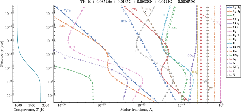
It is important to note that different exoplanets may necessitate the utilization of distinct solar abundances. Nevertheless, the program is compatible with additional datasets that follow the same format as the original dataset abundances.txt (located in the databases folder). The results (solid lines) show an excellent agreement with those obtained with the Thermochemical Equilibrium Abundances (TEA) code [25] (symbols) even down to the bar level. The minor differences in HCN, C2H2 (acetylene), and HSM (the subscript M denotes that is obtained from Burcat’s database) come from the discrepancies of the free energies compared to the NIST-JANAF database [31, 32] that is implemented in TEA. In this test, the computation time with a tolerance of for the molar composition was 0.9 seconds (TEA: 6.42 seconds) for a set of 26 species considered and a total of 90 case studies, which represents a speed-up factor for our code ( loading a specific database for this case).
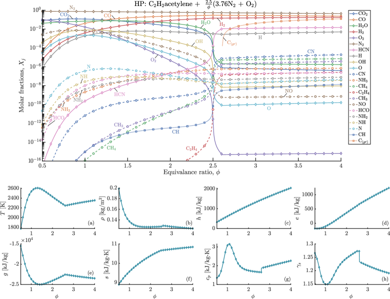
Second test: As previously indicated, thermochemical codes are essential for understanding and predicting the intricate chemical transformations that take place in combustion processes. Therefore, validating CT with a canonical combustion test is critically important. To this end, the second validation test involves the adiabatic isobaric combustion of acetylene and air, a promising mixture for advanced internal combustion engines due to acetylene’s high energy density and low carbon content. Specifically, the investigation focuses on the isobaric reactive mixture at an initial pressure of atm and temperature of K, and considers a wide range of equivalence ratios . Figure 3 shows the variation of the molar composition of the products with (top panel) along with other mixture properties (Figs. 3a-h). It should be noted that, unlike the previous test, in this case the results obtained with CT (represented by solid lines) are compared to those of NASA’s CEA code [17] (represented by symbols). Once again, the results are in excellent agreement with the benchmark code, including the generation of solid carbon C(gr) when the equivalence ratio reaches or exceeds . The computation time elapsed 3.34 seconds for a set of 94 species and 351 case studies, which is faster compared to the previous release [69, 61].
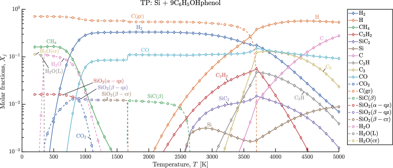
Third test: Recent advancements in chemical equilibrium solvers have opened up new opportunities for studying the complex phenomena that take place on the surface of ablative materials during atmospheric reentry. For instance, Helber et al. [92] used a chemical equilibrium code to investigate the ablation of carbon-based materials under conditions experienced during Earth’s atmospheric reentry. Other studies focused on carbon-fiber-reinforced-polymers (CFRP) [93] or silicon-based ablative materials [94]. Regardless of the composition of the ablator, predicting the equilibrium species generated during the ablation process is a challenging task, as it involves the evaluation of a large number of condensed species at very high enthalpies. To assess the capabilities of CT under more demanding scenarios than those of the previous tests, we recall in this third test the example presented in Ref. [24]. The problem consists of a parametric study of a Si-C6H5OH mixture at atmospheric pressure ( atm) for a wide range of temperatures K. Figure 4 illustrates the variation with temperature of the equilibrium molar fractions for the Silica-Phenolic mixture, along with the results computed using NASA’s CEA code [17]. It can be seen that there is total agreement even for the multiple condensed species. Previous work [24] reported that NASA’s CEA code was not able to converge for K. However, this is only true when computing the parametric study, not the individual cases, whereas CT converges in both situations. In this test, the computation time was 3.05 seconds for a set of 177 species (40 in condensed phase) and 481 case studies, making this version 1.67 faster than the previous release [69, 61].
4 Shock and detonation module
This section presents the routines of the shock and detonation module, CT-SD, which are encapsulated in the ShockSolver and DetonationSolver classes, respectively. These solvers depend on the CT-EQUIL module described above, and therefore, each object is associated with an instance of the EquilibriumSolver class. The CT-SD module determines the post-shock equilibrium state of steady non-reactive and reactive shocks with arbitrary incidence angles, (see inset on the right panel of Fig. 5b). The methods to solve normal shocks and detonation waves, , are based on the algorithm outlined in NASA’s Reference Publication 1311 [17, Chapters 7-9].
4.1 Oblique shocks
First, consider the problem of an undisturbed, planar, normal shock wave. The pre-shock density, pressure, enthalpy, and velocity (in the reference frame attached to the shock) are denoted, respectively, as , , , and . The corresponding flow variables in the post-shock gases are denoted as , , , and . The well-known Rankine-Hugoniot (RH) relations for the variation of pressure and enthalpy are, respectively
| (19) |
These equations must be supplemented by the equation of state, in our case, the ideal EoS , where stands for the average molecular mass of the gaseous mixture computed in terms of the gas-phase molar fractions, , and the molecular masses of the gaseous species, . Also required is the caloric EoS, , that gives enthalpy in terms of the temperature and gas mixture composition. As previously discussed, the molecular masses, , and the molar specific enthalpies, , are evaluated from a combination of NASA’s [33] and Burcat’s (Third Millennium) [34] thermochemical databases.
The solver employs a NR method (see Ref. [17, Chapters 7-9] for more information) to determine the roots of the system of equations governing both reactive and non-reactive shocks (routines detCJ and shockIncident, respectively). Consequently, the jump relationships, such as and , can be calculated with ease. In this subsection, we focus on the oblique shock configuration that implicitly includes the solution of the normal shock wave. When the angle formed by the shock plane and the upstream flow is not , in the RH equations (19) the pre- and post-shock velocities, and , must be replaced by their respective components normal to the shock, and . These equations can be readily reformulated in terms of the magnitudes of the pre- and post-shock velocities upon direct substitution of the trigonometric relationships and , where is the shock incidence angle and is the flow deflection angle, both measured with respect to the upstream flow direction. For oblique shocks, the continuity of the tangential velocity across the shock, , or, equivalently, , is also required.
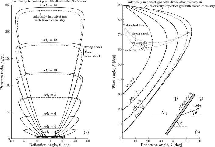
In the case of a normal shock wave, the gas properties downstream of the shock are determined by two factors: the upstream thermodynamic state and a parameter that characterizes the intensity of the shock, usually either the shock speed relative to the upstream gas or the shock Mach number, , where represents the speed of sound upstream the shock. The speed of sound, , is formally defined as . Other problems, such as those concerning blast waves, impose the post-shock pressure as the initial input parameter describing the shock intensity. Oblique shocks, on the other hand, require an additional geometrical restriction given by the value of the incidence angle or the flow deflection angle . It is well known that when the value of is specified, there exists a unique solution for the post-shock fluid state (see routine shockObliqueBeta). However, in the case where is given, there are two possible solutions for : a weak shock solution linked to a smaller value of , representing the weakest possible shock, and a strong solution corresponding to a larger (see routine shockObliqueTheta) [95]. The two solutions converge for , which corresponds to the maximum deflection angle of the shock for a given (see Fig. 5), above which the problem does not admit any solution. Remarkably close to the maximum deflection angle, in the weak-shock branch, we find the sonic condition , below and above which the post-shock flow is supersonic (weak shocks) and subsonic (strong shocks, and weak shocks between the sonic line and the maximum deflection angle), respectively. Then, the supersonic branch always corresponds to the weak shock solution [96].
In either scenario, when the value of is specified, becomes an implicit variable that must be determined numerically. To this end, CT employs an iterative procedure based on the continuity of the tangential velocity across the shock, which can be manipulated using the above trigonometric identities to give
| (20) |
This equation must be solved for the shock incidence angle with use made of the RH relations (19), the ideal gas EoS, and provided that and can be written as explicit functions. This enables the use of Halley’s third-order iterative method [97]
| (21) |
to find the root of Eq. (20). This approach exhibits rapid convergence and meets the default convergence criterion of within two or three iterations. However, it is worth noting that like other root-finding methods, Halley’s method only provides one of the possible roots of the nonlinear system, which generally corresponds to the root closest to the initial guess used during the iterative process. Therefore, we must supply sufficiently accurate guesses to cover the whole set of solutions that include both the weak- and strong-shock branches. One straightforward approach to acquiring such guesses is to anticipate the solution domain bounded by the acoustic weak-shock limit and the normal shock configuration . In particular, we choose for the weak-shock branch and for the strong-shock branch.
The left and right plots in Fig. 5 depict the pressure ratio-deflection angle and the incidence angle-deflection angle shock polar diagrams for dry air (consisting of 78% N2, 21% O2, and 1% Ar) initially at room conditions ( K, atm). These results were obtained using the shockPolar method. It is worth noting that CT provides users with a variety of caloric models to choose from: i) calorically perfect gas with frozen chemistry (constant specific heat at constant pressure , adiabatic index , and ), ii) calorically imperfect gas with frozen chemistry (constant ), and iii) calorically imperfect gas with variable composition, including dissociation, ionization, and recombination reactions at equilibrium. These models are incorporated by specifying a sufficiently large set of species for the calculations, and using NASA’s [33] and Burcat’s (Third Millennium) [34] databases for evaluating the thermodynamic properties.
Figure 5 displays the results obtained with models ii) and iii) spanning a set of pre-shock Mach numbers ranging from 2 to 14. The results are compared with Caltech’s Shock and Detonation Toolbox [67], which uses Cantera [66] as kernel for the computations of chemical equilibrium. It is found that the lobes in the pressure ratio-deflection angle diagram expand due to dissociation/ionization effects, particularly in the hypersonic flow regime, . As a result, weak oblique shocks exhibit smaller pressure ratios while strong ones exhibit larger pressure ratios for the same deflection angle. Moreover, the endothermic (cooling) effect caused by dissociation/ionization in hypersonic oblique shocks leads to an increase in the post-shock density that also increases the wave deflection angle at all incidence angles. The results obtained from both codes are in complete agreement for all conditions tested. However, CT-SD exhibits superior performance compared to Caltech’s SD-Toolbox with Cantera. Our code performs faster on average (CT-SD: 3.78 seconds vs. Caltech’s SD-Toolbox & Cantera: 99.72 seconds; for a large subset that contains 1200 points of all the cases represented in Fig. 5b, with both codes running on the same platform and with the same subset of 13 chemical species), which demonstrates the excellent performance of the CT-SD module.
4.2 Regular reflections
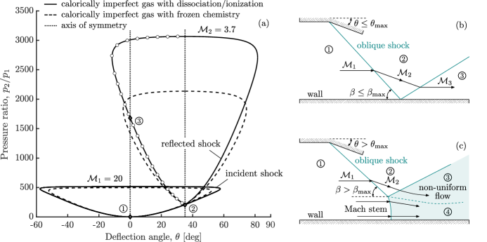
Understanding the reflection of shock waves off flat surfaces is a problem of great relevance to high-speed flows. The angle subtended by the incident shock and the flat surface determines the type of shock reflection, with representing normal reflections and oblique reflections. In a reference frame with origin at the point of contact of the shock with the wall, the latter exhibit an incoming free stream parallel to the wall, with . For sufficiently small incidence angles, the incident shock deflects the free stream uniformly towards the wall an angle . The reflected shock then deflects back the perturbed stream to its original flow direction parallel to the wall. This type of reflection is called regular, and is depicted in Fig. 6b. Regular reflections leave uniform flow patterns behind both the incident and reflected shocks, which can be thoroughly computed using Combustion Toolbox.
By contrast, for incidence angles above a certain critical value, , the reflected wave, characterized by and consequently a lower maximum deflection angle, is not able to deflect the flow back to its upstream direction parallel to the wall. This leads to the so-called irregular, or Mach, reflections, where the reflected and incident shocks merge into a single wave called the Mach stem, which connects the wall to the triple point where the three shocks meet, as illustrated in Fig. 6c. These reflections produce non-uniform flows that include a high-speed shear layer, or slipstream, emanating from the triple point [98]. The properties of these flows cannot be determined solely by the polar-plot charts or the zero-dimensional RH equations and are therefore out of the scope of this work.
To calculate regular reflections, CT-SD uses the routine shockObliqueReflectedTheta to compute the incident wave by specifying the wave angle (or the flow deflection ) and the pre-shock velocity . This results in the calculation of the post-shock state (2), which serves as pre-shock state for the reflected wave (see sketch in Fig. 6b). If the incident shock is sufficiently strong, the transition to state (2) can result in significant thermochemical effects that may cause changes in the aerothermal properties compared to those of a calorically perfect fixed-composition gas. In this case, the values of and may change accordingly. The reflected shock increases the gas pressure and temperature even further, and the properties in state (3) can be determined using the code routine employed for single oblique shocks imposing the counter deflection angle calculated for the incident shock. This guarantees that the streamlines in state (3) are parallel to the reflecting surface. If there is no solution for the reflected shock (which occurs for sufficiently large values of ), irregular Mach reflections occur. As discussed above, these reflections involve non-uniform flow properties and non-steady solutions, and thus their computation is beyond the capabilities of our code.
As an illustrative example, Fig. 6 represents the pressure-deflection shock polar diagrams for a regular shock reflection in atmospheric air at 30 km above sea level with an incident Mach number of and a deflection angle of under the same gas models ii) and iii) used in the oblique shock charts presented previously. The polar plot starting from state (2), obtained by increasing the incident wave angle from 0 to , determines the solution of state (3) for the deflection angle . This, in turn, determines the reflected shock at the intersection of the second polar with the vertical axis (). As can be seen, the dissociation and ionization effects are more pronounced in the reflected shock, as the accumulated temperature jump in both shocks amplifies the endothermicity associated with the dissociation reactions, resulting in substantially higher overall pressure ratios. Finally, the outcomes are compared with those acquired by Zhang et al. [99] under the same flow conditions, revealing excellent agreement in all instances. In our calculations, the computation time was 1.75 seconds for a group of 28 species and 200 case studies. These values depend on the tolerance, which was set to for the root-finding method.
As previously discussed, for each , there exists a maximum value of (and, consequently, of ) beyond which regular reflection is impossible. This maximum value is determined using the shockPolarLimitRR method, which identifies the point where the polar diagram of the reflected shock becomes tangent to the axis. Our code is able to compute and in cases involving high-temperature thermochemical effects. To determine this limit, we impose the condition and employ an iterative algorithm based on Broyden’s method [100], which makes use of the set of routines described above.
4.3 Planar gaseous detonations
The thermochemical framework used to describe shock waves involving endothermic molecular transformations can be easily extended to account for exothermic reactions, as occurs in planar detonations. As with shock waves, the computation of detonations requires knowledge of the pre-shock state and the degree of overdrive that measures the contribution of the external supporting mechanism. However, unlike shock waves, detonations can be self-sustained, i.e., propagate without any external contribution exerting additional pressure from behind. This propagation mode, named after Chapman-Jouguet (CJ), involves the maximum possible expansion of the hot products. Therefore, the burnt-gas state is obtained by imposing the sonic condition in the post-wave flow . If the pressure behind the detonation wave is larger than what is anticipated by the CJ condition, which can only be achieved using an external forcing mechanism, the detonation is considered over-driven and results in subsonic downstream conditions, with . Conversely, under-driven detonations occur when the burnt gas is in a supersonic state with . However, these types of waves are typically disregarded because the post-shock Mach waves within the non-equilibrium region diverge from the oblique shock wave, leading to acoustic decoupling from the wall and making wedge attachment impossible [95]. Further studies also suggest that under-driven detonations may violate the second law of thermodynamics [101]. Nevertheless, since post-detonation equilibrium conditions are independent of the internal structure, under-driven detonations are not excluded by CT when calculating the complete spectrum of possibilities.
The over-driven/under-driven solutions can be determined numerically for a defined upstream mixture and a given degree of overdrive (see functions detOverdriven and detUnderdriven) by using the routines designed for CJ detonations (see detCJ) and normal shocks (see shockIncident). The first routine is needed to determine the minimum velocity (or ) required for a planar detonation to propagate, while the second is used to obtain the post-detonation state for a given degree of overdrive .
Careful selection of the initial guesses is also required to obtain the solutions for over-driven and under-driven detonations. For instance, and denote the estimated temperature and pressure after the detonation front, and should be anticipated considering the significant variations arising from the degree of overdrive and the type of propagation mode. To obtain the initial guesses for over-driven detonations, is computed using Eq. (19), assuming a constant . This gives . The temperature guess is based on the fact that, for sufficiently strong shocks, the kinetic energy downstream is much lower than upstream of the shock, . This simplifies Eq. (19) to , thereby enabling the computation of by solving the thermochemical equilibrium problem at specified enthalpy and pressure, and . This approximation becomes more accurate with increasing degrees of overdrive, as the differences between and become more significant. This estimation method is the same as the one utilized in the incident normal shocks routine. For under-driven detonations, a reasonable initial guess can be obtained by considering the range of acceptable values for the mean post-shock density. By defining the dimensionless parameter to measure how close is to the CJ state compared to the initial state, we can construct an initial guess for the density as follows: . The pressure and temperature values can then be determined using Eq. (19) and the ideal gas EoS, respectively. It has been found that a value of is suitable for the set of Mach numbers tested.
4.4 Oblique gaseous detonations
Detonation waves can also occur in oblique configurations, although they are much less common than oblique shocks. However, oblique detonations are critical in Oblique Detonation Wave Engines (ODWE) [102, 103], where the combustion process occurs across an oblique detonation wave that revolves around a cylindrical combustion chamber.
To compute oblique detonations, knowledge of the pre-shock state and the degree of overdrive caused by the supporting mechanism, typically a wedge deflecting a reactive supersonic stream and generating the oblique detonation, is required, just like in oblique shocks. Thus, given the temperature, pressure, composition, and pre-shock velocity, one can calculate the detonation polar diagrams with the particularity that now the exothermicity of the reaction increases the number of possible solutions, as occurs for planar detonations [104, 105]. Then, for a given detonation angle (or deflection angle ), two solutions for the burnt-gas state can be found, associated with under-driven () and over-driven () conditions (see routines detonationObliqueBeta and detonationObliqueTheta).
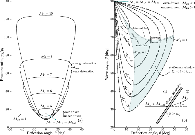
At the Chapman-Jouguet regime the two solutions merge into a single solution. This state is characterized by a sonic normal component of the downstream velocity vector (). The corresponding values for the upstream Mach number and shock angle are and . Both in the under-driven and over-driven cases, the RH-equations only produce real solutions if the values for the upstream Mach number and shock angle are larger than the corresponding values for the CJ condition, and . For oblique detonations with angles in the range , a given shock angle corresponds to two different deflection angles, namely and .
In the over-driven branch, the solution resembles that of an oblique shock. The condition is reached just below the maximum deflection angle separating the strong and weak solutions. Since the solution is multi-valued, the computation of the different branches requires accurate initial guesses regardless of the input parameter, be it the shock or the flow deflection angle (see Section 4.3).
CT provides embedded functionalities for obtaining polar diagrams that characterize incident oblique detonations (see function detPolar). These functionalities perform a direct computation of a set of cases (100 by default) by sweeping the range of possible solutions for both the under-driven and over-driven branches. As an illustrative example, Fig. 7 shows the pressure-deflection (a) and wave angle-deflection (b) polar diagrams for detonations in stoichiometric hydrogen (H2)-air (79% N2, 21% O2) mixtures at pre-shock temperature K and pressure atm, for a range of pre-shock Mach numbers between 5 and 10. The results are compared with those of Zhang et al. [99], which are found to be in remarkable agreement. The computation time was 5.57 seconds for a set of 26 species and 1500 case studies and a tolerance of for the root-finding method. For comparative purposes, the computation time required by Caltech’s SD Toolbox [68] with Cantera [66], which only provides the over-driven branch, was 101.77 seconds. This represents a speed-up factor for our code.
The blue-shaded area shown in Fig. 7 corresponds to weak over-driven conditions, which are the most likely to occur in oblique detonations. This region, bounded by , is of significant interest due to its applicability to the study of ODWE systems [106, 107]. For instance, recent research by Guo et al. [107] investigated the impact of pre-shock conditions on the stationary window for CH4-air oblique detonations. The authors discovered that the limits and depend strongly on the pre-shock velocity and heat release associated with the mixture, while variations with the upstream temperature and pressure are not as prominent. Combustion Toolbox allows to perform these calculations easily, highlighting its relevance in carrying out preliminary studies before tackling more complex flow configurations.
5 Rocket module
The calculation of the theoretical performance of rocket engines has drawn renewed attention in recent times due to the emergence of new private space companies such as Virgin Galactic, SpaceX, Blue Origin, Rocket Lab, or PLD Space, focused on the development of low-cost and reusable launch vehicles [108]. Despite the inherent complexities of these systems associated with the variety of physicochemical phenomena involved, a reasonably accurate estimation of engine performance can be achieved with fairly simple thermochemical calculations. In particular, since rocket engines typically operate at moderate pressures, the ideal gas assumption can be applied without the need for more complex equations of state. Additionally, the long residence times of the reacting gases in the combustion chamber compared to the chemical reaction times allow for further simplification of the calculations. This simplification allows for the utilization of thermochemical equilibrium tools such as CT.
The initial release of CT-ROCKET incorporates the mathematical description proposed in [17], implemented within the RocketSolver class. This method relies on several simplifying assumptions, including one-dimensional flow, uniform cross-sectional area, negligible flow velocity in the combustion chamber inlet, adiabatic combustion, isentropic expansion in the nozzle, homogeneous flow, the ideal gas law, and continuity of temperature and velocity between gaseous and condensed species. Further details on the numerical implementation can be found in Ref. [17, Chapter 6].
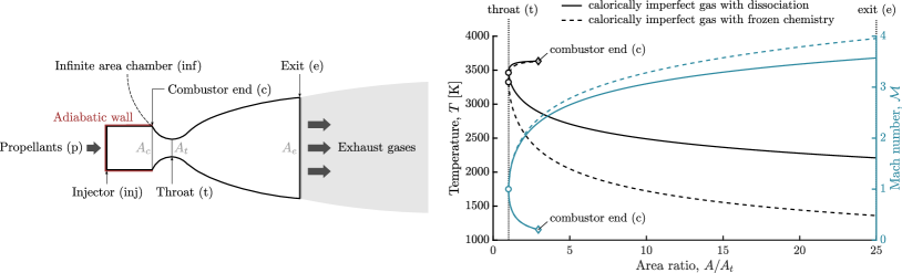
CT-ROCKET leverages the ability of the CT-EQUIL module to determine the gas composition within the rocket engine at various points of interest, such as the injector (inj), the combustion chamber outlet (c), the nozzle throat (t), and different points between (t) and (c/inf) where the hot gases are compressed (subsonic region) or between (t) and the nozzle outlet (e) where the hot gases undergo the final expansion (supersonic region), as illustrated in Fig. 8 (left). The right panel shows the temperature and the Mach number of the fluid particles from the combustion chamber outlet (c) to the exit (e), passing through the throat (t) with , for a LOX/RP1 mixture with equivalence ratio (representing a 2.27 oxidizer/fuel weight ratio) in a high-pressure combustion chamber at atm. The area ratio is taken as the control variable, upon condition that thermochemical equilibrium is achieved at each position.
Additionally, the module calculates the thrust generated by the rocket engine. CT-ROCKET allows for calculations using either frozen chemistry or chemical equilibrium, accounting for combustion chambers with both finite (entropic process) and infinite (isentropic process) dimensions. The frozen chemistry and chemical equilibrium approaches provide an estimate of the performance limits of rocket engine nozzles, as demonstrated by Grossi et al. [109] through two-dimensional numerical simulations based on finite-rate kinetics. This feature enables the performance of parametric analyses to determine the optimal theoretical configuration for a given launch condition or to evaluate the environmental impact at various stages of the rocket vehicle. For instance, with the increasing number of space launches [110, 111], there has been a shift away from highly toxic fuels such as unsymmetrical dimethylhydrazine (UDMH) during the early phases of launch, towards so-called “green” propellants like kerosene (RP1) [112]. It is expected that the use of toxic fuels will be further restricted or even prohibited in the near future, thus driving the need to gain more experience with alternative “green” propellants [113]. The CT-ROCKET module can therefore prove to be a valuable tool in this endeavor.
As previously discussed, this module also includes various routines to compute the state of the mixture at different points of the rocket engine. These states can be modeled using either an infinite area chamber (IAC) or a finite area chamber (FAC) implemented through the rocketIAC and rocketFAC methods, respectively. For example, in the FAC model, an iterative procedure is employed to determine the mixture states at the chamber outlet (c) and at the throat (t). This is achieved by utilizing the IAC model upon defining the initial fresh mixture’s composition, temperature, and pressure, along with the area ratios and .
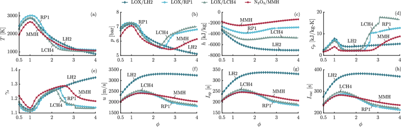
Numerous validations were conducted using NASA’s CEA code to ensure the reliability and robustness of CT-ROCKET. As an example, Fig. 9 displays a range of thermodynamic properties computed at the nozzle exit (e). The geometrical aspect ratios defining the combustion chamber and the nozzle are and . Several reacting mixtures were utilized in the computations, including LOX/LH2, LOX/RP1, LOX/LCH4, and N2O4/MMH, the latter consisting of nitrogen tetroxide and monomethyl-hydrazine. The reactants were introduced in a combustion chamber where they reacted isobarically under high-pressure conditions, atm. The inlet temperature of the propellants was set to their respective boiling points, except for N2O4, which was evaluated at 300 K. The computations were performed over a wide range of equivalence ratios, , to investigate the impact of the fuel-to-oxidizer ratio on the combustion process and the resulting reaction products.
As illustrated in the different subplots of Fig. 9, CT-ROCKET accurately predicts the properties of primary interest at the nozzle exit, including temperature () in (a), pressure () in (b), enthalpy () in (c), specific heat capacity at constant pressure () in (d), adiabatic index () in (e), gas velocity () in (f), specific impulse at sea level () in (g), and specific impulse in a vacuum () in (h). The results demonstrate excellent agreement with the CEA code, with uniform convergence. However, the NASA code exhibited numerical instabilities for certain cases, such as LOX/RP1 at and LOX/LCH4 at . The computation time for LOX/H2 was 11.85 seconds for a set of 11 species and a total of 351 cases. The other mixtures were computed using 94 species, with an average computation time of 30.88 seconds. It is noteworthy that the computation time per species is almost three times less for the latter cases. The performance of the CT-ROCKET module has improved by a factor of compared with the previous release [69, 61].
6 Graphic User Interface
This section presents a detailed overview of the Graphic User Interface (GUI) developed for CT. The GUI is intended to provide a user-friendly and intuitive interface for the visualization and analysis of data. Figures 10 and 11 depict the fundamental elements of the GUI, described in detail below:
-
1.
The menu bar comprises predefined actions such as clear, save, snapshot, and check for updates, along with options to access online documentation, tutorials, examples, and license. It also provides access to additional tools, or add-ons, that can expand the GUI’s capabilities. These add-ons include controls for numerical errors and visualization settings, species selection, as well as the ability to perform code validations and provide feedback to the development team (see CT documentation or its website).
-
2.
The interface is divided into two main tabs (setup and results) and additional sub-tabs designed to organize the content and prevent the user from feeling overwhelmed. The setup tab contains a control panel to configure the problem to be addressed. The results tab contains a data visualization area for post-processing all collected data.
-
3.
The control panel is a crucial part of the GUI that enables users to configure the problem conditions. It provides a range of controls and options to adjust parameters such as the chemical species (reactants and products), the initial state (composition, temperature, and pressure), the type of problem to be solved, and other parameters for the setup of single-case or parametric studies.
-
4.
The command window provides a command-line interface that allows users to interact with the GUI through a series of text commands. This feature is particularly useful for advanced users who prefer to work with code or scripts. Through this tool, users can input commands and execute scripts, while the dialog box prompts the user for further input or confirmation before executing a command. The dialog box displays practical information like warnings, errors, and execution time, providing valuable feedback to the user.
-
5.
The lamp component serves as a visual indicator of the analysis status. When the analysis is complete, the lamp emits a green light, while a yellow light indicates that the computations are still in progress. A red light indicates an error in the analysis.
-
6.
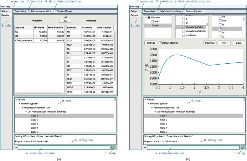
The data visualization area displays the computed results in a visual format, such as plots or tables. It allows users to interact with and explore the data in a way that’s intuitive and easy to understand.
-
7.
The tree component collects all the data and exhibits the hierarchical organization of the obtained outcomes, which enables users to explore and access distinct aspects of each case.
-
8.
Additional features have been incorporated to improve the GUI’s usability, including context menus and keyboard shortcuts. These functionalities enable users to perform intricate tasks with ease and speed.
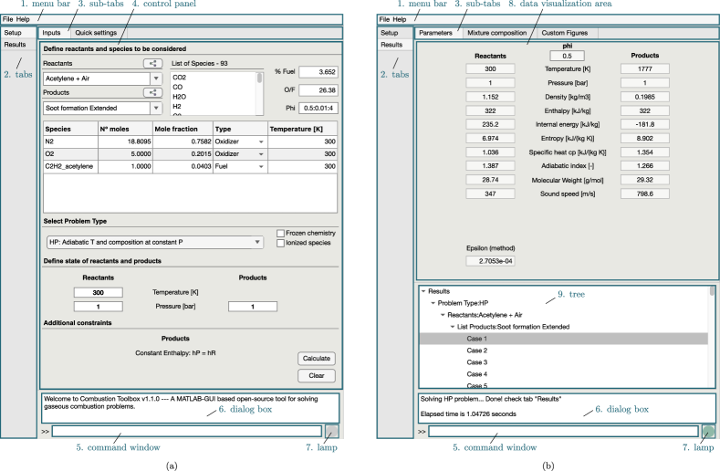
For illustrative purposes, Figs. 10 and 11 show several Combustion Toolbox GUI screenshots captured during the parametric study of adiabatic isobaric combustion of acetylene-air mixtures reported as second validation test in Section 3.4. This case corresponds to the data displayed in Fig. 3. As observed in Fig. 10, the first step involves setting up the problem conditions, which includes i) the initial mixture (composition, temperature, and pressure), that can be chosen from the predefined mixtures via the reactants drop-down menu, or by manually adding the appropriate species name one-by-one to the same object; ii) the problem configuration (adiabatic at constant pressure, etc.); iii) the control parameter for a parametric or individual study, such as the equivalence ratio; and iv) additional input parameters that may be required based on the type of problem.
If a parametric study is selected with the equivalence ratio as the control parameter, the post-processing step can be initiated as depicted in Fig. 10b. If the problem is well-posed, the lamp object will turn green, meaning that the computations were carried out successfully, and a message will appears in the dialog box of the GUI. Subsequently, the obtained dataset is re-structured in the background to fit into the tree object for result post-processing. By selecting each solution of the tree object, the GUI automatically updates the thermodynamic properties of the mixtures in the data visualization area (see Fig. 10). Additionally, in the results custom figures tab, all mixture properties can be analyzed by plotting the results, as illustrated in Fig. 11. The datasets collected using the GUI can also be exported to a structured spreadsheet or .mat file.
In brief, the GUI offers a broad range of tools for examining problems related to chemical equilibrium. The user-friendly design and intuitive features make it accessible to a variety of users, including those with a limited technical background. The GUI is an essential tool for researchers and practitioners who need to perform and analyse extensive parametric studies of the wide range of problems that can be addressed by the code. However, it is important to note that the GUI is intended to supplement traditional coding approaches instead of replacing them. Despite its ability to streamline tasks for non-experts, plain code actually exhibits greater versatility. The GUI itself is constructed upon an existing codebase, whose fundamental functions and calculations are still available for access and manipulation via the command line interface. In fact, proficient users interested in intricate analytical requirements may find that direct coding and execution is a more efficient and effective method than relying exclusively on the GUI. Thus, the GUI ought to be regarded as a tool that assists users with specific tasks rather than as a replacement for the potent and flexible nature of traditional coding.
7 Conclusions
In this work, we present the Combustion Toolbox (CT), an innovative open-source thermochemical code developed for the calculation of equilibrium states in gaseous reacting systems. While CT primarily focuses on combustion problems that may involve the formation of condensed-phase species, its abilities extend to other areas of interest, including the calculation of the atmospheric compositions of gaseous exoplanets, ablation processes, hypersonic shocks, and detonations. CT has been implemented in MATLAB and designed with an object-oriented modular architecture, making it both user- and developer-friendly. Additionally, CT is equipped with an advanced Graphic User Interface that encapsulates the three modules and multiple built-in functions, providing users with a convenient operating experience.
At present, the three modules included in CT are CT-EQUIL, CT-SD, and CT-ROCKET. The first module, CT-EQUIL, is the kernel of the Combustion Toolbox and is responsible for solving the chemical composition of the system at equilibrium. This is achieved by minimizing the Gibbs/Helmholtz free using the Lagrange multiplier approach coupled with a multidimensional Newton-Raphson method. The second module, CT-SD, solves post-shock/detonation states for normal and oblique incident flows, including the computation of reflected waves. The third module, CT-ROCKET, is designed to determine the mixture composition at various points of interest within rocket engines, along with the calculation of the theoretical rocket performance.
The modules have been validated against existing state-of-the-art codes, including NASA’s Chemical Equilibrium with Applications (CEA) [17], Cantera [66] within Caltech’s Shock and Detonation Toolbox (SD-Toolbox) [67, 68], and the newly developed Thermochemical Equilibrium Abundances (TEA) code [25]. All tests showed excellent agreement. As a matter of fact, CT exhibits superior computational performance in terms of cost and time, outperforming Caltech’s SD-Toolbox and TEA by a significant margin. Additional validations can be accessed through the web at https://combustion-toolbox-website.readthedocs.io, which also provides further documentation and examples. The tool is actively maintained and can be accessed at https://github.com/CombustionToolbox/combustion_toolbox.
While the Combustion Toolbox has shown promising results, it is still an ongoing research project that requires additional development to enhance its capabilities. We aim to introduce additional functionalities in future versions of the code, such as the incorporation of non-ideal equations of state (currently under implementation), the analysis of multi-phase systems, a more accurate model for rocket propellant performance, and the extension of the database to include transport properties. We are also considering expanding the code to other well-known open-source programming languages, such as C++ and Python. The former is preferred due to its exceptional performance compared to MATLAB [70], while the latter is desired due to its simplicity [114]. An intermediate step will involve using MEX functions in the kernel of the code to combine C++ and MATLAB for calculating chemical equilibrium at defined temperature and pressure/volume, which is anticipated to substantially improve the speed of the code.
Acknowledgements
The authors acknowledge funding from Comunidad de Madrid under the Multiannual Agreement H2SFE-CM-UC3M. C.H. also received support from projects TED2021-129446B-C41 and PID2022-139082NB-C5 (MICINN/FEDER, UE). M.V. would like to express his lifetime gratitude for the invaluable and inspiring collaborations with Professors Amable Liñán and Antonio L. Sánchez over the past twenty-five years. Their seminal contributions, insight, motivation, and long term support played a pivotal role in initiating and promoting this research effort.
Declaration of Competing Interest
The authors declare that they have no competing financial interests or personal relationships that could have appeared to influence the work reported in this paper.
References
- [1] G. P. Smith, GRI-Mech 3.0, http://www.me.berkley.edu/gri_mech (1999).
- [2] F. J. Zeleznik, S. Gordon, An analytical investigation of three general methods of calculating chemical-equilibrium compositions, National Aeronautics and Space Administration, 1960.
- [3] S. R. Brinkley Jr, Calculation of the equilibrium composition of systems of many constituents, The Journal of Chemical Physics 15 (2) (1947) 107–110. doi:10.1063/1.1746420.
- [4] J. M. Paz-García, B. Johannesson, L. M. Ottosen, A. B. Ribeiro, J. M. Rodríguez-Maroto, Computing multi-species chemical equilibrium with an algorithm based on the reaction extents, Computers & Chemical Engineering 58 (2013) 135–143. doi:10.1016/j.compchemeng.2013.06.013.
- [5] A. M. M. Leal, Reaktoro: An open-source unified framework for modeling chemically reactive systems (2015).
- [6] P. Woitke, C. Helling, G. H. Hunter, J. D. Millard, G. E. Turner, M. Worters, J. Blecic, J. W. Stock, Equilibrium chemistry down to 100 K. Impact of silicates and phyllosilicates on the carbon to oxygen ratio, Astronomy & Astrophysics 614 (2018) A1. doi:10.1051/0004-6361/201732193.
- [7] J. W. Stock, D. Kitzmann, A. B. C. Patzer, E. Sedlmayr, FastChem: A computer program for efficient complex chemical equilibrium calculations in the neutral/ionized gas phase with applications to stellar and planetary atmospheres, Monthly Notices of the Royal Astronomical Society 479 (1) (2018) 865–874. doi:10.1093/mnras/sty1531.
- [8] J. W. Stock, D. Kitzmann, A. B. C. Patzer, FastChem 2: an improved computer program to determine the gas-phase chemical equilibrium composition for arbitrary element distributions, Monthly Notices of the Royal Astronomical Society 517 (3) (2022) 4070–4080. doi:10.1093/mnras/stac2623.
- [9] D. Kitzmann, J. W. Stock, A. B. C. Patzer, FASTCHEM COND: equilibrium chemistry with condensation and rainout for cool planetary and stellar environments, Monthly Notices of the Royal Astronomical Society 527 (3) (2023) 7263–7283. doi:10.1093/mnras/stad3515.
- [10] F. Van Zeggeren, S. H. Storey, The Computation of Chemical Equilibria, Cambridge University Press, Cambridge, 1970.
- [11] W. R. Smith, R. W. Missen, Chemical reaction equilibrium analysis, Wiley, 1982.
- [12] W. B. White, S. M. Johnson, G. B. Dantzig, Chemical equilibrium in complex mixtures, The Journal of Chemical Physics 28 (5) (1958) 751–755. doi:10.1063/1.1744264.
- [13] F. J. Zeleznik, S. Gordon, Calculation of complex chemical equilibria, Industrial & Engineering Chemistry 60 (6) (1968) 27–57. doi:10.1021/ie50702a006.
- [14] G. Eriksson, Thermodynamic studies of high temperature equilibria III. SOLGAS, a computer program for calculating the composition and heat condition of an equilibrium mixture., Acta Chemica Scandinavica 25 (1971) 2651–2658.
- [15] W. C. Reynolds, The element potential method for chemical equilibrium analysis: implementation in the interactive program STANJAN, Technical Rept., Dept. of Mechanical Engineering, Stanford University, 1986 (1986).
- [16] M. L. Michelsen, Calculation of multiphase ideal solution chemical equilibrium, Fluid Phase Equilibria 53 (1989) 73–80. doi:10.1016/0378-3812(89)80073-1.
- [17] S. Gordon, B. J. McBride, Computer program for calculation of complex chemical equilibrium compositions and applications. Part 1: Analysis, No. NAS 1.61:1311 (1994).
- [18] P. Voňka, J. Leitner, Calculation of chemical equilibria in heterogeneous multicomponent systems, Calphad 19 (1) (1995) 25–36. doi:10.1016/0364-5916(95)00004-X.
- [19] L. Eriksson, CHEPP-A chemical equilibrium program package for Matlab, SAE transactions (2004) 730–741, Available: https://www.jstor.org/stable/44740797.
- [20] D. V. Nichita, S. Gomez, E. Luna, Multiphase equilibria calculation by direct minimization of gibbs free energy with a global optimization method, Computers & Chemical Engineering 26 (12) (2002) 1703–1724. doi:10.1016/S0098-1354(02)00144-8.
- [21] S. B. Pope, The computation of constrained and unconstrained equilibrium compositions of ideal gas mixtures using Gibbs function continuation, Cornell University Report FDA (2003) 03–02.
- [22] S. B. Pope, Gibbs function continuation for the stable computation of chemical equilibrium, Combustion and Flame 139 (3) (2004) 222–226. doi:10.1016/j.combustflame.2004.07.008.
- [23] A. Néron, G. Lantagne, B. Marcos, Computation of complex and constrained equilibria by minimization of the gibbs free energy, Chemical engineering science 82 (2012) 260–271. doi:10.1016/j.ces.2012.07.041.
- [24] J. B. Scoggins, T. E. Magin, Gibbs function continuation for linearly constrained multiphase equilibria, Combustion and Flame 162 (12) (2015) 4514–4522. doi:10.1016/j.combustflame.2015.08.027.
- [25] J. Blecic, J. Harrington, M. O. Bowman, TEA: A code calculating thermochemical equilibrium abundances, The Astrophysical Journal Supplement Series 225 (1) (2016) 4 1–14. doi:10.3847/0067-0049/225/1/4.
- [26] J. Gray, J. Chin, T. Hearn, E. Hendricks, T. Lavelle, J. R. Martins, Chemical-Equilibrium Analysis with Adjoint Derivatives for Propulsion Cycle Analysis, Journal of Propulsion and Power 33 (5) (2017) 1041–1052. doi:10.2514/1.B36215.
- [27] C. Tsanas, E. H. Stenby, W. Yan, Calculation of multiphase chemical equilibrium by the modified rand method, Industrial & Engineering Chemistry Research 56 (41) (2017) 11983–11995. doi:10.1021/acs.iecr.7b02714.
- [28] C. Tsanas, E. H. Stenby, W. Yan, Calculation of simultaneous chemical and phase equilibrium by the method of lagrange multipliers, Chemical Engineering Science 174 (2017) 112–126. doi:10.1016/j.ces.2017.08.033.
- [29] J. Coatléven, A. Michel, A successive substitution approach with embedded phase stability for simultaneous chemical and phase equilibrium calculations, Computers & Chemical Engineering (2022) 108041doi:10.1016/j.compchemeng.2022.108041.
- [30] A. Cuadra, C. Huete, M. Vera, Combustion Toolbox: A MATLAB-GUI based open-source tool for solving combustion problems, version 1.1.0 (2024). doi:10.5281/zenodo.5554911.
- [31] M. W. Chase, NIST-JANAF thermochemical tables 4th edition, Journal of Physical and Chemical Reference Data, Monograph 9 (1998) 1529–1564.
- [32] O. V. Dorofeeva, V. P. Novikov, D. B. Neumann, NIST-JANAF thermochemical tables. I. Ten organic molecules related to atmospheric chemistry, Journal of Physical and Chemical Reference Data 30 (2) (2001) 475–513. doi:10.1063/1.1364518.
- [33] B. J. McBride, NASA Glenn coefficients for calculating thermodynamic properties of individual species, National Aeronautics and Space Administration, Glenn Research Center, 2002.
- [34] A. Burcat, B. Ruscic, Third millenium ideal gas and condensed phase thermochemical database for combustion (with update from active thermochemical tables), Tech. rep., Argonne National Lab. (ANL), Argonne, IL (United States) (2005). doi:10.2172/925269.
- [35] B. Ruscic, R. E. Pinzon, G. Von Laszewski, D. Kodeboyina, A. Burcat, D. Leahy, D. Montoy, A. F. Wagner, Active Thermochemical Tables: thermochemistry for the 21st century, in: Journal of Physics: Conference Series, Vol. 16, IOP Publishing, 2005, p. 078. doi:10.1088/1742-6596/16/1/078.
- [36] B. Ruscic, D. H. Bross, Chapter 1 - Thermochemistry, in: T. Faravelli, F. Manenti, E. Ranzi (Eds.), Mathematical Modelling of Gas-Phase Complex Reaction Systems: Pyrolysis and Combustion, Vol. 45 of Computer Aided Chemical Engineering, Elsevier, 2019, pp. 3–114. doi:https://doi.org/10.1016/B978-0-444-64087-1.00001-2.
- [37] J. B. Scoggins, J. Rabinovitch, B. Barros-Fernandez, A. Martin, J. Lachaud, R. L. Jaffe, N. N. Mansour, G. Blanquart, T. E. Magin, Thermodynamic properties of carbon–phenolic gas mixtures, Aerospace Science and Technology 66 (2017) 177–192. doi:10.1016/j.ast.2017.02.025.
- [38] C. F. Goldsmith, G. R. Magoon, W. H. Green, Database of small molecule thermochemistry for combustion, The Journal of Physical Chemistry A 116 (36) (2012) 9033–9057. doi:10.1021/jp303819e.
- [39] G. Blanquart, H. Pitsch, Thermochemical properties of polycyclic aromatic hydrocarbons (pah) from g3mp2b3 calculations, The Journal of Physical Chemistry A 111 (28) (2007) 6510–6520. doi:10.1021/jp068579w.
- [40] G. Blanquart, P. Pepiot-Desjardins, H. Pitsch, Chemical mechanism for high temperature combustion of engine relevant fuels with emphasis on soot precursors, Combustion and Flame 156 (3) (2009) 588–607. doi:10.1016/j.combustflame.2008.12.007.
- [41] K. Narayanaswamy, G. Blanquart, H. Pitsch, A consistent chemical mechanism for oxidation of substituted aromatic species, Combustion and Flame 157 (10) (2010) 1879–1898. doi:10.1016/j.combustflame.2010.07.009.
- [42] G. Blanquart, Effects of spin contamination on estimating bond dissociation energies of polycyclic aromatic hydrocarbons, International Journal of Quantum Chemistry 115 (12) (2015) 796–801. doi:10.1002/qua.24904.
- [43] J. A. Miller, R. J. Kee, C. K. Westbrook, Chemical kinetics and combustion modeling, Annual Review of Physical Chemistry 41 (1) (1990) 345–387.
- [44] N. Kubota, Propellants and explosives: thermochemical aspects of combustion, John Wiley & Sons, 2015.
- [45] C. Huete, A. Cuadra, M. Vera, J. Urzay, Thermochemical effects on hypersonic shock waves interacting with weak turbulence, Physics of Fluids 33 (8) (2021) 086111. doi:10.1063/5.0059948.
- [46] H. Jiang, J. Liu, S. Luo, W. Huang, J. Wang, M. Liu, Thermochemical non-equilibrium effects on hypersonic shock wave/turbulent boundary-layer interaction, Acta Astronautica 192 (2022) 1–14. doi:10.1016/j.actaastro.2021.12.010.
- [47] G. V. Candler, R. W. MacCormack, Computation of weakly ionized hypersonic flows in thermochemical nonequilibrium, Journal of Thermophysics and Heat Transfer 5 (3) (1991) 266–273. doi:10.2514/3.260.
- [48] P. A. Libby, F. A. Williams (Eds.), Turbulent Reacting Flows, Academic Press, New York, 1994.
- [49] P. Wolański, Detonative propulsion, Proceedings of the Combustion Institute 34 (1) (2013) 125–158. doi:10.1016/j.proci.2012.10.005.
- [50] M. Di Renzo, J. Urzay, Direct numerical simulation of a hypersonic transitional boundary layer at suborbital enthalpies, Journal of Fluid Mechanics 912 (2021) A29 1–36. doi:10.1017/jfm.2020.1144.
- [51] V. Raman, S. Prakash, M. Gamba, Nonidealities in rotating detonation engines, Annual Review of Fluid Mechanics 55 (2022). doi:10.1146/annurev-fluid-120720-032612.
- [52] A. Cuadra, C. Huete, M. Vera, Effect of equivalence ratio fluctuations on planar detonation discontinuities, Journal of Fluid Mechanics 903 (2020) A30 1–39. doi:10.1017/jfm.2020.651.
- [53] A. Cuadra, M. Vera, M. Di Renzo, C. Huete, Linear theory of hypersonic shocks interacting with turbulence in air, in: AIAA SciTech 2023 Forum, AIAA paper 2023–0075, 2023. doi:10.2514/6.2023-0075.
- [54] M. Michelsen, Calculation of multiphase equilibrium, Computers & chemical engineering 18 (7) (1994) 545–550. doi:10.1016/0098-1354(93)E0017-4.
- [55] J. B. Scoggins, V. Leroy, G. Bellas-Chatzigeorgis, B. Dias, T. E. Magin, Mutation++: Multicomponent thermodynamic and transport properties for ionized gases in C++, SoftwareX 12 (2020) 100575. doi:10.1016/j.softx.2020.100575.
- [56] A. M. M. Leal, D. A. Kulik, W. R. Smith, M. O. Saar, An overview of computational methods for chemical equilibrium and kinetic calculations for geochemical and reactive transport modeling, Pure and Applied Chemistry 89 (5) (2017) 597–643. doi:10.1515/pac-2016-1107.
- [57] P. J. Groenen, W. J. Heiser, The tunneling method for global optimization in multidimensional scaling, Psychometrika 61 (3) (1996) 529–550. doi:10.1007/BF02294553.
- [58] R. Storn, K. Price, Differential evolution–a simple and efficient heuristic for global optimization over continuous spaces, Journal of Global Gptimization 11 (4) (1997) 341–359. doi:10.1023/A:1008202821328.
- [59] K. V. Price, Differential evolution, in: Handbook of optimization, Springer, 2013, pp. 187–214.
- [60] J. Sánchez-Monreal, A. Cuadra, C. Huete, M. Vera, SimEx: A Tool for the Rapid Evaluation of the Effects of Explosions, Applied Sciences 12 (18) (2022). doi:10.3390/app12189101.
- [61] A. Cuadra, Development of a wide-spectrum thermochemical code with application to planar reacting and non-reacting shocks, PhD thesis, Universidad Carlos III de Madrid, Madrid, Spain, available at http://hdl.handle.net/10016/38179 (May 2023).
- [62] A. Dahake, R. Singh, A. Singh, Dual behavior of hydrogen peroxide in gaseous detonations, Shock Waves 33 (5) (2023) 401–414. doi:10.1007/s00193-023-01142-5.
- [63] J. Chen, M. Sun, P. Li, B. An, W. Jiaoru, M. Li, Effects of excess oxidizer coefficient on RBCC engine performance in ejector mode: A theoretical investigation, Energy 289 (2024) 130070. doi:https://doi.org/10.1016/j.energy.2023.130070.
- [64] C. Xu, H. Ma, X. Yu, Comprehensive performance evaluation method of working fluids for high temperature heat pump based on multi-objective optimization, Applied Thermal Engineering 247 (2024) 123102. doi:10.1016/j.applthermaleng.2024.123102.
- [65] Q. Qin, L. Li, F. Han, Q. Yao, Y. Liu, M. Yuan, X. Li, T. Ji, J. Li, Expansion wave-reinforced initiation of the oblique detonation wave, Physics of Fluids 36 (8) (2024). doi:10.1063/5.0220586.
- [66] D. G. Goodwin, R. L. Speth, H. K. Moffat, B. W. Weber, Cantera: An object-oriented software toolkit for chemical kinetics, thermodynamics, and transport processes, https://www.cantera.org, version 2.5.1 (2021). doi:10.5281/zenodo.4527812.
- [67] S. Browne, J. Ziegler, N. Bitter, B. Schmidt, J. Lawson, J. E. Shepherd, SDToolbox - Numerical Tools for Shock and Detonation Wave Modeling, GALCIT Technical Report FM2018.001 Revised January 2021, California Institute of Technology, Pasadena, CA, https://shepherd.caltech.edu/EDL/PublicResources/sdt (2008).
- [68] S. Browne, J. Ziegler, J. E. Shepherd, Numerical solution methods for shock and detonation jump conditions, GALCIT report FM2006 6 (2008) 1–90.
- [69] A. Cuadra, C. Huete, M. Vera, Combustion Toolbox: A MATLAB-GUI based open-source tool for solving combustion problems, version 1.0.5 (2023). doi:10.5281/zenodo.10581476.
- [70] T. Andrews, Computation time comparison between Matlab and C++ using launch windows, Tech. rep., California Polytechnic State University San Luis Obispo, Available: https://digitalcommons.calpoly.edu/aerosp/78 (2012).
- [71] F. N. Fritsch, R. E. Carlson, Monotone piecewise cubic interpolation, SIAM Journal on Numerical Analysis 17 (2) (1980) 238–246. doi:10.1137/0717021.
- [72] K. Ram, Git can facilitate greater reproducibility and increased transparency in science, Source code for biology and medicine 8 (1) (2013) 1–8. doi:10.1186/1751-0473-8-7.
- [73] S. Chacon, B. Straub, Pro git, Apress, 2014.
- [74] J. D. Blischak, E. R. Davenport, G. Wilson, A quick introduction to version control with git and github, PLOS computational biology 12 (1) (2016) e1004668. doi:10.1371/journal.pcbi.1004668.
- [75] Y. Perez-Riverol, L. Gatto, R. Wang, T. Sachsenberg, J. Uszkoreit, F. da Veiga Leprevost, C. Fufezan, T. Ternent, S. J. Eglen, D. S. Katz, et al., Ten simple rules for taking advantage of git and github (2016). doi:10.1371/journal.pcbi.1004947.
- [76] G. Brandl, Sphinx documentation, Available: http://sphinx-doc.org/sphinx.pdf (2010).
- [77] J. Cederberg, M. Mikofski, jcewidex, D. Rosset, I. Lenton, N. Martin, M. Topper, C. Markiewicz, C. Boeddeker, C. Vergari, cleobis, D. Stansby, florianjacob, PekaryGergelyR, H. Leblanc, M.-H. Bleu-Laine, N. N. Oosterhof, R. Zimmerman, ptitrex, sphinx-contrib/matlabdomain: 0.18.0 (Apr. 2023). doi:10.5281/zenodo.7829592.
- [78] J. Smith, H. Van Ness, et al., Introduction to Chemical Engineering Thermodynamics, McGraw-Hill, 2018.
- [79] D. A. Kulik, T. Wagner, S. V. Dmytrieva, G. Kosakowski, F. F. Hingerl, K. V. Chudnenko, U. R. Berner, GEM-Selektor geochemical modeling package: revised algorithm and GEMS3K numerical kernel for coupled simulation codes, Computational Geosciences 17 (2013) 1–24. doi:10.1007/s10596-012-9310-6.
- [80] A. M. Leal, D. A. Kulik, G. Kosakowski, M. O. Saar, Computational methods for reactive transport modeling: An extended law of mass-action, xlma, method for multiphase equilibrium calculations, Advances in Water Resources 96 (2016) 405–422. doi:10.1016/j.advwatres.2016.08.008.
- [81] D. P. Bertsekas, Constrained Optimization and Lagrange Multiplier Methods, Academic press, New York, 2014.
- [82] E. Anderson, Z. Bai, C. Bischof, L. S. Blackford, J. Demmel, J. Dongarra, J. Du Croz, A. Greenbaum, S. Hammarling, A. McKenney, et al., LAPACK users’ guide, SIAM, 1999.
- [83] B. M. Smirnov, Fundamentals of ionized gases: basic topics in plasma physics, John Wiley & Sons, 2012.
- [84] J. Sharma, A composite third order Newton–Steffensen method for solving nonlinear equations, Applied Mathematics and Computation 169 (1) (2005) 242–246. doi:10.1016/j.amc.2004.10.040.
- [85] B. Fegley Jr, K. Lodders, Atmospheric chemistry of the brown dwarf Gliese 229B: Thermochemical equilibrium predictions, The Astrophysical Journal 472 (1) (1996) L37. doi:10.1086/310356.
- [86] C. Visscher, K. Lodders, B. Fegley Jr, Atmospheric chemistry in giant planets, brown dwarfs, and low-mass dwarf stars. II. Sulfur and phosphorus, The Astrophysical Journal 648 (2) (2006) 1181. doi:10.1086/506245.
- [87] M. Agúndez, V. Parmentier, O. Venot, F. Hersant, F. Selsis, Pseudo 2D chemical model of hot-Jupiter atmospheres: application to HD 209458b and HD 189733b, Astronomy & Astrophysics 564 (2014) A73. doi:10.1051/0004-6361/201322895.
- [88] V. Parmentier, M. R. Line, J. L. Bean, M. Mansfield, L. Kreidberg, R. Lupu, C. Visscher, J.-M. Désert, J. J. Fortney, M. Deleuil, et al., From thermal dissociation to condensation in the atmospheres of ultra hot Jupiters: WASP-121b in context, Astronomy & Astrophysics 617 (2018) A110. doi:10.1051/0004-6361/201833059.
- [89] N. Madhusudhan, Exoplanetary atmospheres: Key insights, challenges, and prospects, Annual Review of Astronomy and Astrophysics 57 (2019) 617–663. doi:10.1146/annurev-astro-081817-051846.
- [90] K. B. Stevenson, J.-M. Désert, M. R. Line, J. L. Bean, J. J. Fortney, A. P. Showman, T. Kataria, L. Kreidberg, P. R. McCullough, G. W. Henry, et al., Thermal structure of an exoplanet atmosphere from phase-resolved emission spectroscopy, Science 346 (6211) (2014) 838–841. doi:10.1126/science.1256758.
- [91] M. Asplund, N. Grevesse, A. J. Sauval, P. Scott, The chemical composition of the sun, Annual Review of Astronomy and Astrophysics 47 (2009) 481–522. doi:10.1146/annurev.astro.46.060407.145222.
- [92] B. Helber, C. O. Asma, Y. Babou, A. Hubin, O. Chazot, T. E. Magin, Material response characterization of a low-density carbon composite ablator in high-enthalpy plasma flows, Journal of materials science 49 (2014) 4530–4543. doi:10.1007/s10853-014-8153-z.
- [93] F. Bariselli, A. Frezzotti, A. Hubin, T. E. Magin, Aerothermodynamic modelling of meteor entry flows, Monthly Notices of the Royal Astronomical Society 492 (2) (2020) 2308–2325. doi:10.1093/mnras/stz3559.
- [94] S.-H. Park, J. N. Laboulais, P. Leyland, S. Mischler, Re-entry survival analysis and ground risk assessment of space debris considering by-products generation, Acta Astronautica 179 (2021) 604–618. doi:10.1016/j.actaastro.2020.09.034.
- [95] D. T. Pratt, J. W. Humphrey, D. E. Glenn, Morphology of standing oblique detonation waves, Journal of Propulsion and Power 7 (5) (1991) 837–845. doi:10.2514/3.23399.
- [96] A. H. Shapiro, The dynamics and thermodynamics of compressible fluid flow, New York: Ronald Press (1953).
- [97] T. Scavo, J. Thoo, On the geometry of halley’s method, The American mathematical monthly 102 (5) (1995) 417–426. doi:doi.org/10.1080/00029890.1995.12004594.
- [98] H. Hornung, Regular and Mach reflection of shock waves, Annual review of fluid mechanics 18 (1986) 33–58. doi:10.1146/annurev.fl.18.010186.000341.
- [99] Z. Zhang, C. Wen, W. Zhang, Y. Liu, Z. Jiang, A theoretical method for solving shock relations coupled with chemical equilibrium and its applications, Chinese Journal of Aeronautics 35 (6) (2022) 47–62. doi:10.1016/j.cja.2021.08.021.
- [100] J. E. Dennis Jr, R. B. Schnabel, Numerical methods for unconstrained optimization and nonlinear equations, SIAM, 1996.
- [101] G. Emanuel, D. G. Tuckness, Steady, oblique, detonation waves, Shock Waves 13 (2004) 445–451. doi:10.1007/s00193-003-0222-1.
- [102] C. Li, K. Kailasanath, E. S. Oran, Detonation structures behind oblique shocks, Physics of Fluids 6 (4) (1994) 1600–1611.
- [103] K. Kailasanath, Review of propulsion applications of detonation waves, AIAA journal 38 (9) (2000) 1698–1708.
- [104] J. M. Powers, K. A. Gonthier, Reaction zone structure for strong, weak overdriven, and weak underdriven oblique detonations, Physics of Fluids A: Fluid Dynamics 4 (9) (1992) 2082–2089.
- [105] Z. Zhang, Y. Liu, C. Wen, Mechanisms of the destabilized Mach reflection of inviscid oblique detonation waves before an expansion corner, Journal of Fluid Mechanics 940 (2022). doi:10.1017/jfm.2022.226.
- [106] X. Zhuo, D. Gang, P. Zhenhua, G. Mingyue, Standing window of oblique detonation with pathological behaviour, Chinese Journal of Aeronautics 34 (5) (2021) 496–503. doi:10.1016/j.cja.2020.12.005.
- [107] H. Guo, N. Zhao, H. Yang, S. Li, H. Zheng, Analysis on stationary window of oblique detonation wave in methane-air mixture, Aerospace Science and Technology 118 (2021) 107038. doi:10.1016/j.ast.2021.107038.
- [108] F. García, M. Nürmberger, R. Torres, J. Crespo, ARION 1 reusable sounding rocket: The new microgravity platform in Europe, Adv. Astronaut. Sci. 1 (1) (2018) 23–30.
- [109] M. Grossi, A. Sereno, D. Bianchi, B. Favini, Role of finite-rate kinetics on the performance predictions of solid rocket motor nozzles, in: AIAA SCITECH 2023 Forum, 2023, p. 1314. doi:10.2514/6.2023-1314.
- [110] H. Jones, The recent large reduction in space launch cost, in: 48th International Conference on Environmental Systems, 2018, pp. 1–12, Available: http://hdl.handle.net/2346/74082.
- [111] I. W. Kokkinakis, D. Drikakis, Atmospheric pollution from rockets, Physics of Fluids 34 (5) (2022) 056107. doi:10.1063/5.0090017.
- [112] A. S. Gohardani, J. Stanojev, A. Demairé, K. Anflo, M. Persson, N. Wingborg, C. Nilsson, Green space propulsion: Opportunities and prospects, Progress in Aerospace Sciences 71 (2014) 128–149. doi:10.1016/j.paerosci.2014.08.001.
- [113] J. Dallas, S. Raval, J. A. Gaitan, S. Saydam, A. Dempster, The environmental impact of emissions from space launches: A comprehensive review, Journal of Cleaner Production 255 (2020) 120209. doi:10.1016/j.jclepro.2020.120209.
- [114] H. Fangohr, A comparison of C, MATLAB, and Python as teaching languages in engineering, in: International Conference on Computational Science, Springer, 2004, pp. 1210–1217. doi:10.1007/978-3-540-25944-2_157.