Fourier analysis of many-body transition amplitudes and states

Abstract

We apply the Fourier transform over the symmetric group $S_{N}$ to the set of multiparticle transition amplitudes arising from the permutations of $N$ identical particles. This allows us to analyse the counting statistics at the output of multiparticle and multimode interference setups in terms of contributions from irreducible symmetry types. We apply our formalism to the interference of partially distinguishable bosons and fermions, whose state can also be submitted to Fourier analysis, and to the determination of suppressed transitions for states of a given symmetry type.

I Introduction

Harmonic analysis is one of the most powerful and versatile tools at the disposal of mathematicians, engineers and physicists. The various flavours of Fourier transformations can notably be put to use to obtain a compact and interpretable representation of complex signals. In particular, the Parseval-Plancherel identity allows to break down the total energy of a wave into contributions from each frequency component. More fundamentally, the Fourier transform provides an analysis of the scales on which the function varies by decomposing it in a basis where translations of its argument act diagonally. Differential and difference equations are thereby mapped onto simpler, algebraic ones. The Fourier transform also holds a prominent place in quantum mechanics since it relates the representations of matter waves in position and momentum space, the two being constrained by the Heisenberg uncertainty relations. In its discrete version, the Fourier transform plays a central role in quantum computing, as it is instrumental in providing an exponential speed-up in resolving so-called hidden subgroup problems, including for example Deutsch’s problem, Simon’s problem and the integer factorization problem.

All of the above applications can be formulated in the language of representation theory of Abelian (i.e. commutative) groups. The Abelian group in question is the group of translations of a given set. Each translation induces a linear map on the vector space of functions defined on that set (or, equivalently, functions defined on the group of translations itself). Since they commute with one another, these maps can be simultaneously diagonalized and the Fourier transform essentially gives the decomposition of a function in the simultaneous eigenbasis. However, the Fourier transform can also be extended to functions defined on a non-commutative finite group. In this case, the action of the group can no longer be simultaneously diagonalized, but representation theory teaches us that it can be broken down into a finite number of elementary operations: the group’s irreducible representations. The Fourier transform decomposes a function over a group in a basis where the group acts irreducibly. The Fourier transform over non-Abelian finite groups has found applications in probability theory and statistics (e.g. to analyse random processes such as the shuffling of a deck of cards) [1, 2], in the study of ranking schemes (e.g. elections) [3, 4], in graph and number theory [5], as well as in machine learning tasks displaying symmetries [6]. The success of the ordinary Fourier transform in practical applications certainly owes a lot to the existence of the Fast Fourier Transform algorithm [7]. By extending its principle to the non-Abelian case [8, 9] , Fourier transforms over finite groups can be computed explicitly despite the rapidly growing size of the involved groups.

In this work, we apply the Fourier transform over the symmetric group $S_{N}$ to the analysis of many-particle interference processes in the dynamics of $N$ identical quantum particles. As a consequence of their indistinguishability, evaluating transition probabilities for $N$ particles requires to consider all $N!$ ways of identifying the particles in the input state with those in the output state. Each such association corresponds to a different many-particle path taken by the system, and has an associated complex transition amplitude. The transition probability thus results from the interference of these $N!$ amplitudes. Furthermore, more often than not, the interfering particles carry internal degrees of freedom which don’t participate in the dynamics but render the particles partially distinguishable from one another [10, 11, 12]. The many-particle transition amplitudes are then dressed by overlaps of these internal states, further adding to the complexity of the interference. On the one hand, uncontrolled partial distinguishability is a source of decoherence in protocols based on many-particle interference, calling for dedicated diagnostics and certification tools [13, 14, 15, 16, 17]. On the other hand, control over the particles’ internal states provides a handle to shape their many-particle interference patterns [18, 19, 20, 21, 22, 23]. We will show that the Fourier transform over the symmetric group provides a natural framework to efficiently characterize partial distinguishability and systematically investigate its effect of on many-particle interference.

Since Weyl and Wigner [24, 25], group theoretical methods have had a long tradition in quantum mechanics — including, but not limited to the description of quantum statistics. In the study of many-particle interference phenomena, previous works have made use of Schur-Weyl duality, which relates irreducible representations of the symmetric group to those of the unitary group [26, 27, 28, 18, 19, 20, 29, 15, 30, 31, 32, 33]. The originality of the present approach is that it makes no reference to the representations of the unitary group. The advantage is that we only need to work with the finite group $S_{N}$, whose irreducible representations can be computed once and for all as they do not depend on the dimension of the single-particle Hilbert space. The result, we hope, is a more transparent picture of many-particle interference.

We start by recalling the definition and main properties of the Fourier transform over a finite group, as well as providing some useful group theory notions. We then proceed with the Fourier analysis of the set of transition amplitudes connecting two $N$-particle states in section III. These are combined into Fourier components associated with specific particle-exchange symmetries, including the familiar bosonic and fermionic symmetries, but also more exotic “mixed” symmetries [35, 36]. In section IV, we study the counting statistics of particles obeying exchange symmetries generalizing those of indistinguishable bosons and fermions. In particular, the transition probabilities of partially distinguishable particles are expressed in terms of the Fourier transforms of the transition amplitudes on the one hand and of a function encoding partial distinguishability on the other hand. As an application of our formalism, in section V, we state conditions for the contribution of a given symmetry type to a transition probability to vanish. This generalizes the suppression laws governing completely destructive interference of bosons and fermions [37, 38, 39, 40, 41, 42, 43, 44, 45] to other symmetry types. We illustrate these results by investigating the spectrum of transition amplitudes in the Fourier interferometer (i.e. for an evolution given by the discrete Fourier transform unitary), where we observe a wealth of such suppressed events.

II Fourier transform over a finite group

The ordinary Fourier transform is the expansion of a function in a basis where all translations of the function’s argument act diagonally. This is possible because translations commute with one another. If we instead consider a non-Abelian group of transformations of the function’s domain, no such basis exists. However, we can find a basis in which the group’s action takes the simplest possible form. The Fourier transform over a finite group performs the corresponding basis change. In this section, we first give the definition of the Fourier transform over a finite group and state its main properties. We then introduce some of the useful mathematical objects which occur in the rest of this work. We assume that the reader is familiar with the basic concepts of group theory and refer to [46, 47, 48] for a more detailed exposition of the representation theory of finite groups.

II.1 Definitions

Consider a group $G$ of finite order $|G|$ whose group operation we denote $\circ$. A $d$-dimensional matrix representation $\rho$ of $G$ is a map

$$\rho:\begin{cases}G&\to GL_{d}(\mathbb{C})\\ \sigma&\mapsto\hat{\rho}(\sigma)\end{cases},$$ (1)

which is compatible with the group operation, i.e. such that

$$\forall\sigma,\tau\in G,\,\hat{\rho}(\sigma\circ\tau)=\hat{\rho}(\sigma)\hat{\rho}(\tau).$$ (2)

Let

$$f:\begin{cases}G&\to\mathbb{C}\\ \sigma&\mapsto f(\sigma)\end{cases}$$ (3)

be a complex-valued function over $G$. The Fourier transform of $f$ over $G$ at the representation $\rho$ is the $d\times d$ matrix

$$\hat{f}(\rho)=\sum_{\sigma\in G}f(\sigma)\hat{\rho}(\sigma).$$ (4)

Note that we use hats to denote matrices in general, for example the representation matrices $\hat{\rho}(\sigma)$ in Eq. (1), and Fourier transforms in particular, for example $\hat{f}$ is the Fourier transform of $f$ in Eq. (4).

A representation $\rho$ of a finite group $G$ can be broken down into a finite set of irreducible representations (irreps) $\rho^{(\lambda)}$ as

$$\rho\simeq\bigoplus_{\lambda}\rho^{(\lambda)}\otimes\mathbb{I}_{m_{\lambda}},$$ (5)

i.e., in an appropriately chosen basis (here $\simeq$ denotes equality up to a basis change), the matrices $\hat{\rho}(\sigma)$ are all block-diagonal, with the block $\hat{\rho}^{(\lambda)}(\sigma)$ appearing $m_{\lambda}$ times. The irrep matrices $\hat{\rho}^{(\lambda)}$ are unique up to a change of basis. The knowledge of the Fourier transform $\hat{f}$ at a complete set of irreps $\rho^{(\lambda)}$ of $G$ allows to recover the original function through the inverse transform

$$f(\sigma)=\sum_{\lambda}\frac{d_{\lambda}}{|G|}\operatorname{Tr}\left[\hat{\rho}^{(\lambda)}(\sigma^{-1})\hat{f}(\lambda)\right],$$ (6)

where $d_{\lambda}$ is the irrep’s dimension. For simplicity, we write $\hat{f}(\lambda)$ for $\hat{f}(\rho^{(\lambda)})$, the Fourier transform at the irrep with label $\lambda$. In essence, the individual entries of the matrix irreps form an orthogonal basis of the space of complex-valued functions on $G$ and Eq. (6) is the expansion of $f$ in that basis [see Appendix A for details].

We recover the ordinary (discrete) Fourier transform in the case where $G$ is a cyclic group. Without loss of generality, we take $G=\{0,1,\dots|G|-1\}$, with the group operation given by addition modulo $|G|$. Since $G$ is Abelian, its irreps are all one-dimensional and are given by the group characters $\hat{\rho}^{(\lambda)}(\sigma)=\chi^{(\lambda)}(\sigma)=\exp(2\mathrm{i}\pi\lambda\sigma/|G|)$, where both $\sigma$ and $\lambda$ run from $0$ to $|G|-1$. The Fourier transform [Eq. (4)] and its inverse [Eq. (6)] then take the familiar forms

$$\hat{f}(\lambda)=\sum_{\sigma=0}^{|G|-1}f(\sigma)\exp(2\mathrm{i}\pi\lambda\sigma/|G|)$$ (7)

and

$$f(\sigma)=\frac{1}{|G|}\sum_{\lambda=0}^{|G|-1}\hat{f}(\lambda)\exp(-2\mathrm{i}\pi\lambda\sigma/|G|).$$ (8)

$\bm{\sigma\mapsto\tau^{-1}\circ\sigma}$

Symmetric group $S_{3}$
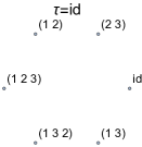
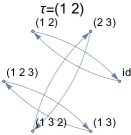
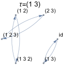
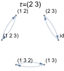
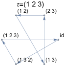
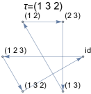
Cyclic group of order 6

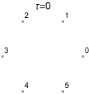
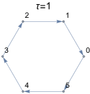
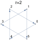
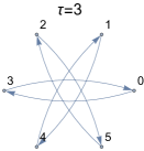
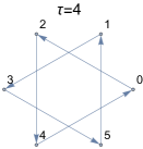
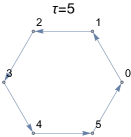
Figure 1: Graphical representations of the multiplication tables of the (non-Abelian) group $S_{3}$ (top) and the (Abelian) cyclic group of order 6 (bottom). The group elements $\sigma$ are represented by points on a circle. For each group element $\tau$, the map $\sigma\mapsto\tau^{-1}\circ\sigma$ is depicted by arrows connecting these points.

Let us take the group of permutations of three elements, i.e the symmetric group $S_{3}$, as a simple example. It has $3!=6$ elements $\sigma$, which we write using cycle notation ($\operatorname{id}$ being the identity permutation). The multiplication table of $S_{3}$ is schematically represented in the top row of Fig. 1. The elements $\sigma$ of $S_{3}$ are represented by six points on a circle. For each permutation $\tau\in S_{3}$, we connect these points according to the map $\sigma\mapsto\tau^{-1}\circ\sigma$. These transformations do not commute in general. To contrast, we also show the corresponding diagrams for the cyclic group of order six in the second row of Fig. 1. In that case, compositions by a group element corresponds to translations along the ring, which commute with one another. The symmetric group $S_{3}$ must therefore possess an irrep $\lambda$ with $d_{\lambda}>1$. This is the two-dimensional standard irrep. It also has two one-dimensional irreps, the trivial and sign irreps (irreps of the symmetric group are discussed in more detail in Sec. III.2). The corresponding matrices $\hat{\rho}^{(\lambda)}(\sigma)$ can be taken as follows:

$\sigma$	$\operatorname{id}$	$(1\,2)$	$(1\,3)$	$(2\,3)$	$(1\,2\,3)$	$(1\,3\,2)$
$\hat{\rho}^{(\mathrm{triv})}(\sigma)$	$(1)$	$(1)$	$(1)$	$(1)$	$(1)$	$(1)$
$\hat{\rho}^{(\mathrm{stand})}(\sigma)$	$\begin{pmatrix}1&0\\ 0&1\end{pmatrix}$	$\begin{pmatrix}1&0\\ 0&-1\end{pmatrix}$	$\dfrac{1}{2}\begin{pmatrix}1&-\sqrt{3}\\ -\sqrt{3}&-1\end{pmatrix}$	$\dfrac{1}{2}\begin{pmatrix}1&\sqrt{3}\\ \sqrt{3}&-1\end{pmatrix}$	$\dfrac{1}{2}\begin{pmatrix}-1&-\sqrt{3}\\ \sqrt{3}&-1\end{pmatrix}$	$\dfrac{1}{2}\begin{pmatrix}-1&\sqrt{3}\\ -\sqrt{3}&-1\end{pmatrix}$
$\hat{\rho}^{(\mathrm{sign})}(\sigma)$	$(1)$	$(-1)$	$(-1)$	$(-1)$	$(1)$	$(1)$

II.2 Basic operations

The Fourier transform over a finite group $G$ [Eq. (4)] enjoys the following properties:

• Shifting the argument of $f$ by a group element $\tau\in G$ (as sketched in Fig. 1) corresponds to multiplying its Fourier transform $\hat{f}(\rho)$ by $\hat{\rho}(\tau)$, specifically

  $$\text{if}\quad f_{\tau}:\sigma\mapsto f(\tau^{-1}\circ\sigma),\quad\text{then}\quad\hat{f_{\tau}}(\rho)=\hat{\rho}(\tau)\hat{f}(\rho).$$ (9)

• The “convolution product” $f*g$ of two functions $f$ and $g$, defined by

  $$\forall\sigma\in G,\qquad(f*g)(\sigma)=\sum_{\tau\in G}f(\sigma\circ\tau^{-1})g(\tau)=\sum_{\tau\in G}f(\tau)g(\tau^{-1}\circ\sigma),$$ (10)

  is mapped to the matrix product of $\hat{f}$ and $\hat{g}$, i.e. for any representation $\rho$,

  $$\widehat{f*g}(\rho)=\hat{f}(\rho)\hat{g}(\rho).$$ (11)

• The “scalar product” $(f,g)$ of two functions $f$ and $g$, defined by

  $$(f,g)=\sum_{\sigma\in G}f(\sigma^{-1})g(\sigma),$$ (12)

  can be expressed in terms of their Fourier transforms with the help of the Parseval-Plancherel identity:

  $$(f,g)=\sum_{\lambda}\frac{d_{\lambda}}{|G|}\operatorname{Tr}\left[\hat{f}(\lambda)\hat{g}(\lambda)\right].$$ (13)

  Note that Eq. (12) does not define an inner product in the strict sense, since $(f,g)=(g,f)$ is in general not equal to its complex conjugate $(g,f)^{*}$. Therefore $(f,f)$ need not be real, let alone positive. If we introduce the function $f^{\star}$ such that $f^{\star}(\sigma)=f(\sigma^{-1})^{*}$ for all $\sigma\in G$, we can define a proper inner product $\left\{f,g\right\}=(f^{\star},g)$. In particular, $\left\{f,f\right\}=(f^{\star},f)=\sum_{\sigma\in G}|f(\sigma)|^{2}$ is strictly positive for $f\neq 0$. If $\rho$ is a unitary representation, i.e. the inverse $\hat{\rho}(\sigma^{-1})$ of $\hat{\rho}(\sigma)$ is equal to its conjugate-transpose $\hat{\rho}(\sigma)^{\dagger}$, then $\widehat{f^{\star}}(\rho)=\hat{f}(\rho)^{\dagger}$ and

  $$\left\{f,g\right\}=\sum_{\lambda}\frac{d_{\lambda}}{|G|}\operatorname{Tr}\left[\hat{f}(\lambda)^{\dagger}\hat{g}(\lambda)\right]$$ (14)

  is a (weighted) sum over the Hilbert-Schmidt products of $\hat{f}$ and $\hat{g}$ taken at each irrep.

• If we combine the convolution and scalar products to form a “triple product”, we have, as a consequence of the two previous points

  $$(f*g,h)=\sum_{\lambda}\frac{d_{\lambda}}{|G|}\operatorname{Tr}\left[\hat{f}(\lambda)\hat{g}(\lambda)\hat{h}(\lambda)\right]=(g*h,f)=(f,g*h),$$ (15)

  i.e. the triple product is invariant under cyclic permutations of its three arguments and under exchange of the two products.

II.3 Class functions and isotypic projectors

Class functions are defined over the conjugacy classes of $G$, i.e. they take the same value at $\sigma\in G$ and at all elements $\sigma^{\prime}=\tau\circ\sigma\circ\tau^{-1},\,\tau\in G,$ of its conjugacy class. We can also express this as condition as follows: for $c$ a class function,

$$c(\tau\circ\sigma)=c(\sigma\circ\tau)\qquad\forall\sigma,\tau\in G.$$ (16)

As a consequence, class functions are in the center of the algebra defined by the convolution product Eq. (10), i.e. for all functions $f$ on $G$ and all class functions $c$, we have $c*f=f*c$.

Let $\delta_{\tau}$ be the function which evaluates to one at a given $\tau\in G$ and to zero elsewhere, i.e. $\delta_{\tau}(\sigma)=\delta_{\tau,\sigma}$ for all $\sigma\in G$. Setting $f=\delta_{\tau}$ in the above commutation relation and taking the Fourier transform of at an irrep $\lambda$, we find that $\hat{c}(\lambda)\hat{\rho}^{(\lambda)}(\tau)=\hat{\rho}^{(\lambda)}(\tau)\hat{c}(\lambda)$ for all $\tau\in G$, i.e. $\hat{c}(\lambda)$ is a so-called intertwiner. From Schur’s lemma [46, 47, 48], it follows that $\hat{c}(\lambda)$ is proportional to the identity, i.e.

$$\hat{c}(\lambda)=c_{\lambda}\hat{\mathbb{I}}_{d_{\lambda}}$$ (17)

for a constant $c_{\lambda}$.

Group characters $\chi(\sigma)=\operatorname{Tr}(\hat{\rho}(\sigma))$ are a prominent example of class functions which additionally satisfy $\chi^{\star}=\chi$, i.e. $\chi(\sigma^{-1})=\chi(\sigma)^{*}$. In particular, as a consequence of the orthogonality theorem [see Appendix A], the Fourier transform of the complex conjugate of the irreducible character $\chi^{(\mu)}$ at irrep $\lambda$ reads

$$\widehat{\chi^{(\mu)*}}(\lambda)=\sum_{\sigma\in G}\chi^{(\mu)}(\sigma^{-1})\hat{\rho}^{(\lambda)}(\sigma)=\frac{|G|}{d_{\lambda}}\delta_{\mu,\lambda}\hat{\mathbb{I}}_{d_{\lambda}},$$ (18)

i.e. the coefficients $c_{\lambda}$ [Eq. (17)] vanish for all but $\lambda=\mu$. If $\rho$ is a reducible representation, we can thus define the projector on its irreducible subrepresentations of type $\mu$ — the so-called isotypic projection — as

$$\hat{P}^{(\mu)}(\rho)=\frac{d_{\mu}}{|G|}\sum_{\sigma\in G}\chi^{(\mu)}(\sigma^{-1})\hat{\rho}(\sigma),$$ (19)

such that

$$\hat{P}^{(\mu)}(\lambda)=\delta_{\mu,\lambda}\hat{\mathbb{I}}_{d_{\lambda}}.$$ (20)

The isotypic projectors obey

$$\hat{P}^{(\lambda)}(\rho)\hat{P}^{(\mu)}(\rho)=\delta_{\lambda,\mu}\hat{P}^{(\lambda)}(\rho)\qquad\text{and}\qquad\sum_{\lambda}\hat{P}^{(\lambda)}(\rho)=\hat{\mathbb{I}}_{d}.$$ (21)

If $\rho$ is unitary, i.e. $\hat{\rho}(\sigma^{-1})=\hat{\rho}(\sigma)^{\dagger}$, they are also Hermitian:

$$\hat{P}^{(\lambda)}(\rho)^{\dagger}=\hat{P}^{(\lambda)}(\rho),$$ (22)

i.e. they decompose the full representation space into mutually orthogonal subspaces.

Every group $G$ possesses a one-dimensional trivial irrep $\rho^{(\text{triv})}$ such that $\hat{\rho}^{(\text{triv})}(\sigma)=\chi^{(\text{triv})}(\sigma)=1$ for all $\sigma\in G$. The isotypic projector on the trivial components of a representation $\rho$ is thus given by

$$\hat{P}^{(\text{triv})}(\rho)=\frac{1}{|G|}\sum_{\sigma\in G}\hat{\rho}(\sigma)$$ (23)

and the multiplicity of the trivial irrep in the representation $\rho$ is

$$m_{\text{triv}}=\operatorname{Tr}[\hat{P}^{(\text{triv})}(\rho)]=\frac{1}{|G|}\sum_{\sigma\in G}\chi(\sigma).$$ (24)

II.4 Coset decomposition and fast transform

If $G$ has a subgroup $H$, it can be partitioned into $|G|/|H|$ left cosets $\sigma_{i}H$, $i=1,\dots|G|/|H|$, where the $\sigma_{i}\in G$ are coset representatives. Every element $\sigma\in G$ thus belongs to a unique coset $\sigma_{i}H$, i.e. there is a unique $\tau\in H$ such that $\sigma=\sigma_{i}\circ\tau$. We can therefore write the Fourier transform Eq. (4) as

$$\hat{f}(\rho) =\sum_{i=1}^{|G|/|H|}\hat{\rho}(\sigma_{i})\sum_{\tau\in H}f(\sigma_{i}\circ\tau)\hat{\rho}(\tau).$$ (25)

Denoting the set of left cosets of $H$ in $G$ by $G/H$, we also write (slightly abusively) $\sigma\in G/H$ to signify that $\sigma$ runs over a set of representatives of the cosets (a transversal), such that the above becomes

$$\hat{f}(\rho) =\sum_{\sigma\in G/H}\hat{\rho}(\sigma)\sum_{\tau\in H}f(\sigma\circ\tau)\hat{\rho}(\tau).$$ (26)

Analogously, one can use the partition of $G$ into the set $H\backslash G$ of right cosets $H\sigma$ to write

$$\hat{f}(\rho) =\sum_{\sigma\in H\backslash G}\left(\sum_{\tau\in H}f(\tau\circ\sigma)\hat{\rho}(\tau)\right)\hat{\rho}(\sigma).$$ (27)

The inner sums in Eqs. (26)-(27) are Fourier transforms over $H$ of shifted versions of $f$. In this way, the Fourier transform can be iteratively evaluated on representations of smaller groups, generalizing the well-known Fast Fourier Transform algorithm for the efficient evaluation of ordinary discrete Fourier transforms [8, 9].

For $H$ a subgroup in $G$, we define its normalized indicator function $I_{H}$ such that

$$I_{H}(\sigma)=\frac{1}{|H|}\quad\text{if }\sigma\in H\quad\text{and}\quad I_{H}(\sigma)=\ 0\quad\text{otherwise.}$$ (28)

Convolution of a function $f$ with $I_{H}$ performs an averaging over cosets of $H$:

$$(f*I_{H})(\sigma) =\frac{1}{|H|}\sum_{\tau\in H}f(\sigma\circ\tau^{-1})=\frac{1}{|H|}\sum_{\pi\in\sigma H}f(\pi),$$ (29)

$$(I_{H}*f)(\sigma) =\frac{1}{|H|}\sum_{\tau\in H}f(\tau^{-1}\circ\sigma)=\frac{1}{|H|}\sum_{\pi\in H\sigma}f(\pi).$$ (30)

As a consequence, if $f$ is constant on the left cosets of $H$, then

$$f*I_{H}=f,$$ (31)

and similarly,

$$I_{H}*f=f$$ (32)

if $f$ is constant on the right cosets of $H$. In particular, we have

$$I_{H}*I_{H}=I_{H},$$ (33)

such that the Fourier transform $\hat{I}_{H}(\rho)$ is a projector. Evaluating this Fourier transform at an irrep $\lambda$ yields

$$\hat{I}_{H}(\lambda)=\frac{1}{|H|}\sum_{\sigma\in H}\hat{\rho}^{(\lambda)}(\sigma),$$ (34)

which we recognize as the isotypic projector on the trivial components of the restriction $\rho^{(\lambda)}\Big{|}_{H}$ of the irrep $\lambda$ of $G$ to $H$. In particular, $\hat{I}_{H}(\lambda)$ vanishes if the trivial irrep does not appear in the decomposition of $\rho^{(\lambda)}\Big{|}_{H}$. As we have seen in the previous section, this is the case if and only if

$$\operatorname{Tr}\left[\hat{I}_{H}(\lambda)\right]=0,\qquad\text{i.e., }\qquad\sum_{\sigma\in H}\chi^{(\lambda)}(\sigma)=0.$$ (35)

Given Eqs. (31) and (32), the above provides a sufficient condition for $\hat{f}(\lambda)$ to vanish if $f$ is constant over left or right cosets of $H$.

III Many-particle transition amplitudes

We now move on to the topic of this work, namely the quantum interference of identical particles. Consider $N$ identical particles, each endowed with an $M$-dimensional single-particle Hilbert space $\mathcal{H}$ spanned by a set of orthogonal modes $\{\ket{0},\dots\ket{M-1}\}$. The $N$-particle Hilbert space $\mathcal{H}^{\otimes N}$, of dimension $M^{N}$, has basis vectors $\ket{\bm{m}}=\ket{m_{1}}\otimes\ket{m_{2}}\otimes\dots\ket{m_{N}}$, with $m_{\alpha}\in\{0,\dots M-1\}$ for $\alpha=1,\dots N$ (note that we count the modes from $0$ to $M-1$ while particles are labelled from $1$ to $N$). It carries a unitary representation $R$ of the symmetric group $S_{N}$, with a permutation $\sigma\in S_{N}$ acting on $N$-particle basis states by reordering the factors of the tensor product:

$$\hat{R}(\sigma)\ket{\bm{m}}=\hat{R}(\sigma)\ket{m_{1}}\otimes\ket{m_{2}}\otimes\dots\ket{m_{N}}=\ket{m_{\sigma^{-1}(1)}}\otimes\ket{m_{\sigma^{-1}(2)}}\otimes\dots\ket{m_{\sigma^{-1}(N)}}.$$ (36)

III.1 Transition amplitude function

Our many-particle system is assumed to undergo a non-interacting, unitary evolution, which we can think of as scattering through a linear $M$-port interferometer. The evolution thus maps a basis state $\ket{\bm{m}}$ to

$$U^{\otimes N}\ket{\bm{m}}=(U\ket{m_{1}})\otimes(U\ket{m_{2}})\otimes\dots(U\ket{m_{N}}),$$ (37)

where $U\in U(M)$ is a unitary transformation of $\mathcal{H}$. The many-particle transition amplitude between an input basis state $\ket{\bm{i}}$ and an output basis state $\ket{\bm{o}}$ thus factorizes as

$$\braket{\bm{o}}{U^{\otimes N}}{\bm{i}}=\prod_{\alpha=1}^{N}\braket{o_{\alpha}}{U}{i_{\alpha}}.$$ (38)

However, in the quantum evolution of identical particles, it might not be possible to unambiguously identify each particle in the output state with a particle in the input state. It is thus necessary to also consider the amplitudes of transitions to states where the particles are permuted. We therefore define the transition amplitude function

$$a:\begin{cases}S_{N}&\to\mathbb{C}\\ \sigma&\mapsto a(\sigma)=\braket{\bm{o}}{\hat{R}(\sigma)^{\dagger}U^{\otimes N}}{\bm{i}}\end{cases}$$ (39)

giving the transition amplitude between $\ket{\bm{i}}$ and $\hat{R}(\sigma)\ket{\bm{o}}$ for each permutation $\sigma\in S_{N}$. Note that we do not need to additionally consider permutations of the input state since permutation operators commute with the evolution operator $U^{\otimes N}$, so that

$$\forall\sigma,\tau\in S_{N},\qquad\braket{\bm{o}}{\hat{R}(\sigma)^{\dagger}U^{\otimes N}\hat{R}(\tau)}{\bm{i}}=\braket{\bm{o}}{\hat{R}(\tau^{-1}\circ\sigma)^{\dagger}U^{\otimes N}}{\bm{i}}=a(\tau^{-1}\circ\sigma).$$ (40)

At this point, we should note that most of the results of this work do not rely on the dynamics being non-interacting, i.e. on the factorization of the $N$-particle evolution operator $\mathcal{U}=U^{\otimes N}$. Indeed, the only requirement to apply our formalism is the commutation of $\mathcal{U}$ with all permutations $\hat{R}(\sigma)$. In other words, the evolution should not distinguish between the particles, but it can have them interact. Keeping this in mind, we nevertheless proceed with a non-interacting evolution to better connect to the existing literature in the field of photonic interference.

The function $a$ and its Fourier transform $\hat{a}$ over $S_{N}$ will be the main objects of this work. While both contain the same information, the latter has the double advantage that the symmetric group acts upon it in a transparent way [Eq. (9)] and that it allows for an analysis in terms of the irreps of $S_{N}$. For example, consider two arbitrary superpositions of states with the same occupations (i.e. number of particles per mode) as $\ket{\bm{i}}$ and $\ket{\bm{o}}$:

$$\hat{c}(R)\ket{\bm{i}}=\sum_{\sigma\in S_{N}}c(\sigma)\hat{R}(\sigma)\ket{\bm{i}}\quad\text{and}\quad\hat{d}(R)\ket{\bm{o}}=\sum_{\sigma\in S_{N}}d(\sigma)\hat{R}(\sigma)\ket{\bm{o}},$$ (41)

where the complex functions $c$ and $d$ over $S_{N}$ define the coefficients of the superpositions (leaving out normalization for the time being). Fourier transforms over $S_{N}$ at the representation $R$, such as $\hat{c}(R)$ above, will occur repeatedly in the following. To lighten the notation, we omit the representation $R$ whenever there is no risk of confusion, and simply write $\hat{c}\ket{\bm{i}}$ for $\hat{c}(R)\ket{\bm{i}}$.

The transition amplitude between $\hat{c}\ket{\bm{i}}$ and $\hat{d}\ket{\bm{o}}$ can be successively written as

$$\braket{\bm{o}}{\hat{d}^{\dagger}U^{\otimes N}\hat{c}}{\bm{i}} =\braket{\bm{o}}{\widehat{d^{\star}*c}\,U^{\otimes N}}{\bm{n}}$$ (42)

$$=\sum_{\sigma\in S_{N}}(d^{\star}*c)(\sigma)\braket{\bm{o}}{\hat{R}(\sigma)U^{\otimes N}}{\bm{n}}$$ (43)

$$=(a,d^{\star}*c)$$ (44)

$$=\sum_{\lambda}\frac{d_{\lambda}}{N!}\operatorname{Tr}\left[\hat{c}(\lambda)\hat{a}(\lambda)\hat{d}(\lambda)^{\dagger}\right],$$ (45)

where we have expressed our result in terms of a scalar product [Eq. (12)] such that we could make use of the Parseval-Plancherel identity [Eq (13)]. Clearly, the class of states defined in Eq. (41) contains bosonic and fermionic states as special cases, corresponding to the choices $c(\sigma)=d(\sigma)=1$ and $c(\sigma)=d(\sigma)=\operatorname{sign}(\sigma)$, respectively. In the following, we discuss other possible symmetry types.

III.2 Irreps of the symmetric group

To proceed, let us review the irreducible representations of the symmetric group, which appear in the sum Eq. (45). Again, we refer the reader to [46, 47, 48] for details. Irreps of $S_{N}$ are indexed by integer partitions of $N$, $\lambda=(\lambda_{1},\lambda_{2},\dots\lambda_{r})$, with integers $\lambda_{1}\geq\lambda_{2}\dots\geq\lambda_{r}>0$ such that $\sum_{k=1}^{r}\lambda_{k}=N$, which can be represented by Young diagrams with $N$ boxes. For example, the Young diagram associated with the irrep $\lambda=(2,1,1)$ of $S_{4}$ is

boxsize=1em 2,1,1

The dimension $d_{\lambda}$ of irrep $\lambda$ is equal to the number of standard Young tableaux of shape $\lambda$ and is given by the hook-length formula [47]. The matrices $\hat{\rho}^{(\lambda)}(\sigma)$ can be taken real and orthogonal, such that the characters $\chi^{(\lambda)}(\sigma)$ are real and obey $\chi^{(\lambda)}(\sigma^{-1})=\chi^{(\lambda)}(\sigma)$.

The symmetric group has two one-dimensional irreps:

• The trivial irrep, associated with the partition $\lambda=(N)$, is such that $\hat{\rho}^{(N)}(\sigma)=\chi^{(N)}(\sigma)=1$. The corresponding projector $\hat{P}^{(N)}=\frac{1}{N!}\sum_{\sigma\in S_{N}}\hat{R}(\sigma)$ is the symmetrizer, which projects onto completely symmetric $N$-particle states, i.e. states of $N$ bosons.

• The sign irrep, associated with the partition $\lambda=(1,1,\dots 1)$, is such that $\hat{\rho}^{(1,\dots)}(\sigma)=\chi^{(1,\dots)}(\sigma)=\operatorname{sign}(\sigma)$. The corresponding projector $\hat{P}^{(1,\dots)}=\frac{1}{N!}\sum_{\sigma\in S_{N}}\operatorname{sign}(\sigma)\hat{R}(\sigma)$ is the antisymmetrizer, which projects onto completely antisymmetric $N$-particle states, i.e. states of $N$ fermions.

A prominent irrep beyond the aforementioned one-dimensional irreps is the $(N-1)$-dimensional standard irrep, associated with the partition $\lambda=(N-1,1)$. It is conveniently obtained as a subrepresentation of the permutation representation $r$, which acts on vectors $\bm{c}=(c_{1},\dots c_{N})\in\mathbb{C}^{N}$ by permuting their coordinates:

$$\hat{r}(\sigma)\bm{c}=\hat{r}(\sigma)(c_{1},\dots c_{N})=(c_{\sigma^{-1}(1)},\dots c_{\sigma^{-1}(N)}).$$ (46)

It is clear that the vector $\bm{s}=(1,\dots 1)$ carries the trivial (bosonic) irrep $\lambda=(N)$, since $\forall\sigma\in S_{N},\ \hat{r}(\sigma)\bm{s}=\bm{s}$. Its complement, the hyperplane orthogonal to $\bm{s}$, transforms according to the standard irrep. The character of the permutation representation $\chi^{(r)}(\sigma)=\operatorname{Tr}(\hat{r}(\sigma))$ is given by the number of fixed points of the permutation $\sigma$. Since we have the decomposition $\chi^{(r)}(\sigma)=\chi^{(N)}(\sigma)+\chi^{(N-1,1)}(\sigma)=1+\chi^{(N-1,1)}(\sigma)$, the irreducible character $\chi^{(N-1,1)}(\sigma)$ is therefore given by the number of fixed points of $\sigma$ minus one. Taking the tensor product of an irrep $\lambda$ with the sign irrep [i.e. multiplying it by $\operatorname{sign}(\sigma)$] yields its conjugate irrep $\overline{\lambda}$, whose Young diagram is obtained from $\lambda$ by transposition. For example, the bosonic and fermionic irreps are conjugate and the irrep $\lambda=(2,1\dots,1)$ is obtained by multiplying the sign and standard irreps.

Given that bosonic and fermionic states are associated with the trivial and sign irreps of the symmetric group, respectively, it is natural to also consider many-particle states which transform according to other irreps $\lambda$, i.e. particles whose exchange symmetry is neither totally symmetric nor totally antisymmetric [35, 36]. As for bosons and fermions, states with mixed symmetry are obtained by applying the corresponding projector $\hat{P}^{(\lambda)}$ on an arbitrary state, provided the result does not vanish. Note that while mixed symmetries generalize those of bosons and fermions, they are distinct from anyonic symmetries, which correspond to irreps of the braiding group, rather than those of the symmetric group. Mixed-symmetry states are conceptually closer to the notion of paraparticles, particles whose states transform according to specific subsets of irreps $\lambda$ of $S_{N}$ [49, 50]. While they do not seem to be realized at an elementary level in nature, many-particle states with an mixed symmetry can be engineered by suitably entangling distinguishable entities. This symmetry is then preserved by any further evolution which does not distinguish these entities, offering robustness against global noise sources. Moreover, as we will discuss in detail further on, mixed symmetries are relevant for the discussion of systems of partially distinguishable bosons or fermions.

III.3 Generalized Pauli principle

Applying the symmetrization operator $\hat{P}^{(N)}$ to an arbitrary basis state $\ket{\bm{m}}$ always gives a non-zero result. In the case of the antisymmetrizer $\hat{P}^{(1,\dots)}$, on the other hand, it is well known that Pauli’s exclusion principle applies: $P^{(1,\dots)}\ket{\bm{m}}$ vanishes as soon as a given mode appears more than once in $\ket{\bm{m}}$. For mixed symmetries, the condition $P^{(\lambda)}\ket{\bm{m}}\neq 0$ enforces a generalized Pauli principle [36].

A necessary and sufficient condition for $P^{(\lambda)}\ket{\bm{m}}\neq 0$ is given by Gamas’ theorem [52, 53, 54]: it must be possible to write the mode labels $m_{\alpha}$ appearing in state $\ket{\bm{m}}$ in the boxes of the Young diagram $\lambda$ such that no label appears twice in the same column. For the Young diagram $\lambda=(N)$ with a single row, this is trivially always possible. For the Young diagram $\lambda=(1,\dots)$ with a single column, no mode should appear twice. For other symmetry types, no more than $\lambda_{1}$ particles should occupy the same mode, no more than $\lambda_{1}+\lambda_{2}$ particles should occupy the same pair of modes, and so on. In particular, $P^{(\lambda)}\ket{\bm{m}}=0$ whenever $\lambda$ has more than $M$ rows. As an example, for $N=4$ and $\lambda=(2,1,1)$, $P^{(\lambda)}\ket{0,0,1,2}\neq 0$ since we can fill the corresponding Young diagram as follows

boxsize=1em00,1,2

but $P^{(\lambda)}\ket{0,0,1,1}=0$ since it is impossible to fill the first column of the Young diagram without repeating one of the mode labels.

The generalized Pauli principle can equivalently be formulated as a condition on the restriction $\rho^{(\lambda)}\Big{|}_{\operatorname{stab}(\bm{m})}$ of the irrep $\lambda$ of $S_{N}$ to the stabilizer of $\ket{\bm{m}}$, i.e. the subgroup of $S_{N}$ which leaves $\ket{\bm{m}}$ invariant:

$$\operatorname{stab}(\bm{m})=\{\sigma\in S_{N}:\hat{R}(\sigma)\ket{\bm{m}}=\ket{\bm{m}}\}.$$ (47)

The stabilizer of $\ket{\bm{m}}$ consists of all permutations of particles occupying the same mode, therefore its cardinality is $|\operatorname{stab}(\bm{m})|=\prod_{m=0}^{M-1}n_{m}!$, where $n_{m}$ is the number of time mode $m$ appears in $\bm{m}$. It forms a so-called Young subgroup of $S_{N}$, which is isomorphic to the product $S_{n_{0}}\times S_{n_{1}}\times\dots S_{n_{M-1}}$. We have

$$\left\|\hat{P}^{(\lambda)}\ket{\bm{m}}\right\|^{2}=\braket{\bm{m}}{\hat{P}^{(\lambda)}}{\bm{m}}=\frac{d_{\lambda}}{N!}\sum_{\sigma\in S_{N}}\chi^{(\lambda)}(\sigma)\braket{\bm{m}}{\hat{R}(\sigma)}{\bm{m}}=\frac{d_{\lambda}}{N!}\sum_{\sigma\in\operatorname{stab}(\bm{m})}\chi^{(\lambda)}(\sigma),$$ (48)

such that $\hat{P}^{(\lambda)}\ket{\bm{m}}$ vanishes if and only if the trivial irrep does not appear in $\rho^{(\lambda)}\Big{|}_{\operatorname{stab}(\bm{m})}$ (recall Sec. II.4). This in turn means that $I_{\bm{m}}=I_{\operatorname{stab}(\bm{m})}$, the normalized indicator function of the stabilizer of $\ket{\bm{m}}$, has a vanishing Fourier transform at irrep $\lambda$:

$$\hat{I}_{\bm{m}}(\lambda)=\frac{1}{|\operatorname{stab}(\bm{m})|}\sum_{\sigma\in\operatorname{stab}(\bm{m})}\hat{\rho}^{(\lambda)}(\sigma)=0.$$ (49)

For the transition amplitude function $a$ between states $\ket{\bm{i}}$ and $\ket{\bm{o}}$ [Eq. (39)], it holds that

$$\forall\tau\in\operatorname{stab}(\bm{o}),\ \forall\pi\in\operatorname{stab}(\bm{i}),\ \forall\sigma\in S_{N},\qquad a(\tau\circ\sigma\circ\pi)=a(\sigma).$$ (50)

In other words, $a$ is constant on each of the double-cosets $\operatorname{stab}(\bm{o})\sigma\operatorname{stab}(\bm{i})$. It follows that

$$a =I_{\bm{i}}*a*I_{\bm{o}}$$ (51)

and

$$\hat{a}(\lambda) =\hat{I}_{\bm{i}}(\lambda)\hat{a}(\lambda)\hat{I}_{\bm{o}}(\lambda).$$ (52)

Therefore $\hat{a}(\lambda)$ vanishes if $\hat{I}_{\bm{i}}(\lambda)=0$ or $\hat{I}_{\bm{o}}(\lambda)=0$, i.e. if either $\ket{\bm{i}}$ or $\ket{\bm{o}}$ does not comply with the generalized Pauli principle for irrep $\lambda$. Such forbidden combinations of $\bm{i}$, $\bm{o}$ and $\lambda$ are marked in blue in Figs 2-4.

III.4 Permanent, determinant and immanants

Let us now compute the transition amplitude between two mixed-symmetry states $\hat{P}^{(\lambda)}\ket{\bm{i}}$ and $\hat{P}^{(\mu)}\ket{\bm{o}}$. Given the properties of the projectors [Eq. (21)],

$$\braket{\bm{o}}{\hat{P}^{(\mu)}{}^{\dagger}U^{\otimes N}\hat{P}^{(\lambda)}}{\bm{i}}=\delta_{\lambda,\mu}\braket{\bm{o}}{U^{\otimes N}\hat{P}^{(\lambda)}}{\bm{i}}$$ (53)

must vanish if the input and output state do not share the same symmetry. Moreover, with Eqs. (20) and (45), we can write

$$\braket{\bm{o}}{U^{\otimes N}\hat{P}^{(\lambda)}}{\bm{i}}=\frac{d_{\lambda}}{N!}\operatorname{Tr}\left[\hat{a}(\lambda)\right].$$ (54)

The transition amplitude between states of symmetry $\lambda$ is thus given by the the trace of the Fourier transform $\hat{a}(\lambda)$ of the transition amplitude function Eq. (39) at irrep $\lambda$. Furthermore, this trace

$$\operatorname{Tr}\left[\hat{a}(\lambda)\right]=\sum_{\sigma\in S_{N}}\chi^{(\lambda)}(\sigma)a(\sigma)=\operatorname{imm}^{(\lambda)}\mathcal{A}$$ (55)

is the immanant of the $N$-particle scattering matrix $\mathcal{A}$ with entries $\mathcal{A}_{\alpha,\beta}=\braket{o_{\alpha}}{U}{i_{\beta}},\alpha,\beta=1,\dots N$, defined by

$$\text{imm}^{\lambda}(\mathcal{A})=\sum_{\sigma\in S_{N}}\chi^{(\lambda)}(\sigma)\prod_{\alpha=1}^{N}\mathcal{A}_{\alpha,\sigma(\alpha)}.$$ (56)

For the trivial and sign irreps, the immanant coincides with the permanent and determinant, respectively, and we immediately recover well-known results for bosonic and fermionic transition amplitudes:

$$\braket{\bm{o}}{\hat{P}^{(N)}{}^{\dagger}U^{\otimes N}\hat{P}^{(N)}}{\bm{i}} =\frac{1}{N!}\hat{a}(N)=\frac{1}{N!}\operatorname{perm}\mathcal{A},$$ (57)

$$\braket{\bm{o}}{\hat{P}^{(1,\dots)}{}^{\dagger}U^{\otimes N}\hat{P}^{(1,\dots)}}{\bm{i}} =\frac{1}{N!}\hat{a}(1,\dots)=\frac{1}{N!}\det\mathcal{A}.$$ (58)

Note that the bosonic and fermionic transition amplitudes are invariant (up to a sign for fermions) under arbitrary permutations of the input and/or output states, by virtue of

$$\hat{\rho}^{(N)}(\sigma)\hat{a}(N) =\hat{a}(N)\hat{\rho}^{(N)}(\sigma)=\hat{a}(N),$$ (59)

$$\hat{\rho}^{(1,\dots)}(\sigma)\hat{a}(1,\dots) =\hat{a}(1,\dots)\hat{\rho}^{(1,\dots)}(\sigma)=\operatorname{sign}(\sigma)\hat{a}(1,\dots).$$ (60)

However, this does not hold for general transition amplitudes of the form of Eq. (54). Instead, these are only invariant under a common permutation of $\ket{\bm{i}}$ and $\ket{\bm{o}}$, since

$$\operatorname{Tr}\left[\hat{\rho}^{(\lambda)}(\tau)\hat{a}(\lambda)\hat{\rho}^{(\lambda)}(\tau)^{\dagger}\right]=\operatorname{Tr}\left[\hat{a}(\lambda)\right]$$ (61)

by cyclicity of the trace and unitarity of $\rho^{(\lambda)}$.

We can also consider transitions between more general mixed-symmetry states with the same occupations as $\ket{\bm{i}}$ and $\ket{\bm{o}}$ by applying the projection operator $\hat{P}^{(\lambda)}$ to arbitrary superpositions $\hat{c}\ket{\bm{i}}$ and $\hat{d}\ket{\bm{o}}$. We then obtain

$$\braket{\bm{o}}{\hat{d}^{\dagger}\hat{P}^{(\lambda)}{}^{\dagger}U^{\otimes N}\hat{P}^{(\lambda)}\hat{c}}{\bm{i}}=\frac{d_{\lambda}}{N!}\operatorname{Tr}\left[\hat{c}(\lambda)\hat{a}(\lambda)\hat{d}^{\dagger}(\lambda)\right]$$ (62)

which is different from Eq. (54) in general. Indeed, apart from the bosonic and fermionic cases, states of a given symmetry $\lambda$ are not uniquely defined by the number of particles in each mode.

IV Counting statistics in many-particle interference

In practice, many-particle interference experiments measure counting statistics at the output of an interferometer, i.e. the probability distribution over events where a given number of particles is found in each output port, or marginals thereof. Specifically, we want to evaluate the probability $P_{\{n_{m}\}}$ of measuring $n_{m}$ particles in output mode $m$ for each $m=0,\dots M-1$. To do so, we define the (ordered) state

$$\ket{\bm{o}}=\ket{\underbrace{0,\dots 0}_{n_{0}},\underbrace{1,\dots 1}_{n_{1}}\dots,\underbrace{M-1\dots}_{n_{M-1}}}$$ (63)

and form the projector on the set of distinct permutations of $\ket{\bm{o}}$,

$$P_{\bm{o}} =\frac{1}{|\operatorname{stab}(\bm{o})|}\sum_{\sigma\in S_{N}}\hat{R}(\sigma)\ket{\bm{o}}\bra{\bm{o}}\hat{R}(\sigma)^{\dagger},$$ (64)

whose expectation value in the output state yields the desired probability. In the following, we express such probabilities, for particles obeying different types of statistics, in terms of Fourier-transformed transition amplitude functions. In particular, we consider the case of partially distinguishable bosons and fermions, and we will see that their states can also be submitted to a Fourier analysis.

IV.1 Bosons, fermions, mixed symmetries and distinguishable particles

We start with an arbitrary initial state with input mode occupations specified by the mode list $\bm{i}$, which we again write as $\hat{c}(R)\ket{\bm{i}}$ for some function $c$ on $S_{N}$. After a non-interacting evolution, the probability $P_{\{n_{m}\}}$ is given by

$$P_{\{n_{m}\}}=\frac{\braket{\bm{i}}{\hat{c}^{\dagger}U^{\dagger\otimes N}P_{\bm{o}}U^{\otimes N}\hat{c}}{\bm{i}}}{\braket{\bm{i}}{\hat{c}^{\dagger}\hat{c}}{\bm{i}}}.$$ (65)

With the help of the Parseval-Plancherel relation, we can express the numerator and denominator in terms of Fourier transforms [see Appendix. B], yielding

$$P_{\{n_{m}\}} =\frac{1}{|\operatorname{stab}(\bm{i})||\operatorname{stab}(\bm{o})|}\frac{\sum_{\lambda}d_{\lambda}\operatorname{Tr}\left[\hat{a}^{\dagger}(\lambda)\hat{c}^{\dagger}(\lambda)\hat{c}(\lambda)\hat{a}(\lambda)\right]}{\sum_{\lambda}d_{\lambda}\operatorname{Tr}\left[\hat{I}_{\bm{i}}(\lambda)\hat{c}^{\dagger}(\lambda)\hat{c}(\lambda)\right]}.$$ (66)

We obtain the counting statistics of states with symmetry $\lambda$ (including the bosonic and fermionic cases) by letting $\hat{c}=\hat{P}^{(\lambda)}\hat{d}$, which singles out a single term in the sums over irreps:

$$P_{\{n_{m}\}}=\frac{1}{|\operatorname{stab}(\bm{i})||\operatorname{stab}(\bm{o})|}\frac{\operatorname{Tr}\left[\hat{a}^{\dagger}(\lambda)\hat{d}^{\dagger}(\lambda)\hat{d}(\lambda)\hat{a}(\lambda)\right]}{\operatorname{Tr}\left[\hat{I}_{\bm{i}}(\lambda)\hat{d}^{\dagger}(\lambda)\hat{d}(\lambda)\right]}.$$ (67)

In particular, if $\hat{d}(R)=\hat{\delta}_{\sigma}(R)=\hat{R}(\sigma)$ simply permutes the state $\ket{\bm{i}}$ with $\sigma$, then $\hat{d}^{\dagger}(\lambda)\hat{d}(\lambda)=\hat{\mathbb{I}}_{d_{\lambda}}$ and

$$P_{\{n_{m}\}}=\frac{1}{|\operatorname{stab}(\bm{i})||\operatorname{stab}(\bm{o})|}\frac{\operatorname{Tr}\left[\hat{a}^{\dagger}(\lambda)\hat{a}(\lambda)\right]}{\operatorname{Tr}\left[\hat{I}_{\bm{i}}(\lambda)\right]}.$$ (68)

To make the connection to the results of Sec. III.4, note that

$$\operatorname{Tr}\left[\hat{a}^{\dagger}(\lambda)\hat{a}(\lambda)\right]=\left((\chi^{(\lambda)}*a)^{\star},\chi^{(\lambda)}*a\right)=\sum_{\sigma\in S_{N}}\left|\sum_{\tau\in S_{N}}\chi^{(\lambda)}(\tau)a(\tau^{-1}\circ\sigma)\right|^{2}=\sum_{\sigma\in S_{N}}\left|\operatorname{imm}^{(\lambda)}(\mathcal{A}_{\sigma})\right|^{2},$$ (69)

where $\mathcal{A}_{\sigma}$ is obtained from the scattering matrix $\mathcal{A}$ by permuting its rows with $\sigma$. We recognize the transition probability associated with the transition amplitude (55), summed over all output states with the same occupations as $\ket{\bm{o}}$.

To obtain the counting statistics of distinguishable particles, we instead take $\hat{c}=\hat{\mathbb{I}}$ in Eq. (66), yielding

$$P_{\{n_{m}\}}=\braket{\bm{i}}{U^{\dagger\otimes N}P_{\bm{o}}U^{\otimes N}}{\bm{i}}=\frac{1}{|\operatorname{stab}(\bm{o})|}\sum_{\lambda}\frac{d_{\lambda}}{N!}\operatorname{Tr}\left[\hat{a}^{\dagger}(\lambda)\hat{a}(\lambda)\right].$$ (70)

Rewriting the above transition probability as

$$P_{\{n_{m}\}}=\frac{1}{|\operatorname{stab}(\bm{o})|}(a^{\star},a)=\frac{1}{|\operatorname{stab}(\bm{o})|}\sum_{\sigma\in S_{N}}|a(\sigma)|^{2}=\frac{1}{|\operatorname{stab}(\bm{o})|}\operatorname{perm}|\mathcal{A}|^{2},$$ (71)

where $|\cdot|^{2}$ denotes taking the modulus square element-wise, we recover the well-known fact that the transition probabilities of distinguishable particles can be expressed as permanents of matrices with positive entries.

IV.2 Partially distinguishable bosons and fermions

While particles displaying a single mixed permutation symmetry $\lambda$ remain rather hypothetical objects, mixed symmetries are central to a topic of great practical relevance: the study of partial distinguishability in systems of bosons or fermions. Partially distinguishable particles posses internal states which act as ambiguous labels: if they are distinct enough, they allow to identify the particles, many-particle paths become distinguishable from one another and many-particle interference is suppressed; if they are similar, they do not unequivocally individuate the particles and interference is restored [12]. To describe partially distinguishable particles, we extend the single-particle Hilbert space $\mathcal{H}$ by taking its the tensor product with an internal state space $\mathcal{I}$. The $N$-particle Hilbert space can then be decomposed as $\left(\mathcal{H}\otimes\mathcal{I}\right)^{\otimes N}\simeq\mathcal{H}^{\otimes N}\otimes\mathcal{I}^{\otimes N}$. A bosonic or fermionic state on this full $N$-particle Hilbert space reduces to a state of partially distinguishable bosons or fermions on $\mathcal{H}^{\otimes N}$ upon tracing out the internal degrees of freedom.

Bosonic and fermionic $N$-particle states $\varrho_{\mathrm{tot}}$ on $\mathcal{H}^{\otimes N}\otimes\mathcal{I}^{\otimes N}$ are defined by the condition

$$\forall\sigma\in S_{N},\quad\hat{R}(\sigma)\otimes\hat{R}_{\mathrm{int}}(\sigma)\varrho_{\mathrm{tot}}=\epsilon(\sigma)\varrho_{\mathrm{tot}}$$ (72)

where the representation $R_{\mathrm{int}}$ acts on $\mathcal{I}^{\otimes N}$ in the same way as $R$ acts on $\mathcal{H}^{\otimes N}$ [see Eq. (36)] and with $\epsilon(\sigma)=1$ for bosons and $\epsilon(\sigma)=\operatorname{sign}(\sigma)$ for fermions. In particular, we have, for all permutations $\sigma$,

$$\hat{R}(\sigma)\otimes\hat{R}_{\mathrm{int}}(\sigma)\varrho_{\mathrm{tot}}\hat{R}(\sigma)^{\dagger}\otimes\hat{R}_{\mathrm{int}}(\sigma)^{\dagger}=\varrho_{\mathrm{tot}}.$$ (73)

If we are only interested in the evolution and measurement of the external degrees of freedom of the $N$ particles, we can trace out $\mathcal{I}^{\otimes N}$ to obtain the reduced external state

$$\varrho=\operatorname{Tr}_{\mathrm{int}}(\varrho_{\mathrm{tot}}).$$ (74)

Taking the trace over internal degrees of freedom on both sides of Eq. (73), we find that the external state satisfies

$$\forall\sigma\in S_{N},\qquad\hat{R}(\sigma)\varrho\hat{R}(\sigma)^{\dagger}=\varrho,$$ (75)

i.e., it commutes with the permutation operators.

If the external mode occupations are fixed, the state $\varrho$ is supported on the subspace of $\mathcal{H}^{\otimes N}$ spanned by states of the form $\hat{R}(\sigma)\ket{\bm{i}}$ for a given mode list $\bm{i}$ and $\sigma$ running over $S_{N}$. Thanks to the commutation property Eq. (75), all non-vanishing matrix elements of $\varrho$ are encoded in a single partial distinguishability function $j:S_{N}\to\mathbb{C}$, defined in analogy with the transition amplitude function of Eq. (39) by

$$j:\sigma\mapsto\frac{N!}{|\operatorname{stab}(\bm{i})|}\braket{\bm{i}}{\hat{R}(\sigma)^{\dagger}\varrho}{\bm{i}}.$$ (76)

Given $j$, one can reconstruct $\varrho$ as

$$\varrho=\frac{1}{N!|\operatorname{stab}(\bm{i})|}\sum_{\sigma,\tau\in S_{N}}j(\tau^{-1}\circ\sigma)\hat{R}(\sigma)\ket{\bm{i}}\bra{\bm{i}}\hat{R}^{\dagger}(\tau).$$ (77)

The Fourier transform $\hat{j}$ of the partial distinguishability function — together with that of the transition amplitude function $a$— can then be used to express the transition probability of partially distinguishable particles to states with occupations $n_{m}$ corresponding to the mode list $\bm{o}$ [see Appendix. B]:

$$P_{\{n_{m}\}}=\operatorname{Tr}(U^{\otimes N}\varrho U^{\dagger\otimes N}P_{\bm{o}})=\frac{1}{|\operatorname{stab}(\bm{o})||\operatorname{stab}(\bm{i})|}\sum_{\lambda}\frac{d_{\lambda}}{N!}\operatorname{Tr}\left[\hat{a}^{\dagger}(\lambda)\hat{j}(\lambda)\hat{a}(\lambda)\right].$$ (78)

The Fourier transform $\hat{j}(\lambda)$ also provide an analysis of the state in terms of its behaviour under particle permutations, allowing for a meaningful characterization of its partial distinguishability. One can for example compute [see Appendix C] the weight of the state on symmetry sector $\lambda$ as

$$p_{\lambda} =\operatorname{Tr}\left[\varrho\hat{P}^{(\lambda)(R)}\right]=\frac{d_{\lambda}}{N!}\operatorname{Tr}[\hat{j}(\lambda)],$$ (79)

and the purity of $\varrho$ as

$$\operatorname{Tr}\left[\varrho^{2}\right]=\frac{1}{N!}\sum_{\lambda}\frac{d_{\lambda}}{N!}\operatorname{Tr}\left[\hat{j}(\lambda)^{2}\right].$$ (80)

These quantities are essential to quantify the partial distinguishability of the particles [10, 12, 33]. In particular, the projection $p_{(N)}=\hat{j}(N)/N!$ on the bosonic sector is considered as a measure of bosonic indistinguihsability in a number of works [11, 55, 56]. However, the collection of Fourier transforms $\hat{j}(\lambda)$ also contains all higher-order information about the state. For example, for bosons that are close to being indistinguishable, we can expect that $\hat{j}(N-1,1)$ contains the most relevant information on deviations from indistinguishability. By focusing on a few relevant sectors $\lambda$, we can thus achieve a characterization of partial distinguishability that is more detailed than that given by the single number $\hat{j}(N)$, but more economical than the full information contained in the $N!$ matrix elements $j(\sigma)$.

Let us note at this point that the matrices $\hat{j}(\lambda)$ inherit the Hermiticity and positivity of the state $\varrho$. The former property follows from

$$j^{\star}(\sigma) =j(\sigma^{-1})^{*}=\frac{1}{N!|\operatorname{stab}(\bm{i})|}\braket{\bm{i}}{\hat{R}(\sigma^{-1})^{\dagger}\varrho}{\bm{i}}^{*}=\frac{1}{N!|\operatorname{stab}(\bm{i})|}\braket{\bm{i}}{\hat{R}(\sigma)^{\dagger}\varrho}{\bm{i}}=j(\sigma),$$ (81)

where we have made use of $\varrho^{\dagger}=\varrho$ and of Eq. (75). The positivity of $\hat{j}(\lambda)$ is less obvious to prove, and we do so in Appendix D.

To see more explicitly how $j$ relates to the internal states of the particles, let us consider an arbitrary $N$-particle internal state described by a density operator $\varrho_{\mathrm{int}}$ on $\mathcal{I}^{\otimes N}$ and form the following bosonic or fermionic state with input mode occupations given by the mode list $\bm{i}$:

$$\varrho_{\text{tot}}=\mathcal{N}\hat{S}_{\epsilon}\left(\ket{\bm{i}}\bra{\bm{i}}\otimes\varrho_{\mathrm{int}}\right)\hat{S}_{\epsilon}^{\dagger}.$$ (82)

Here $\mathcal{N}$ is a normalization constant such that $\operatorname{Tr}(\varrho_{\text{tot}})=1$ and the (anti)symmetrizer is given by

$$\hat{S}_{\epsilon}=\frac{1}{N!}\sum_{\sigma\in S_{N}}\epsilon(\sigma)\hat{R}(\sigma)\otimes\hat{R}_{\mathrm{int}}(\sigma)=\hat{S}_{\epsilon}^{\dagger}.$$ (83)

A short calculation gives

$$j=\frac{I_{\bm{i}}*J*I_{\bm{i}}}{(I_{\bm{i}},J)},$$ (84)

where the function

$$J(\sigma)=\epsilon(\sigma)\operatorname{Tr}\left[\varrho_{\text{int}}\hat{R}_{\mathrm{int}}(\sigma)\right],\qquad\sigma\in S_{N},$$ (85)

which was introduced in [57, 10, 55, 58], depends only on the internal state $\varrho_{\mathrm{int}}$ and — through $\epsilon$— on the quantum statistics of the particles. In terms of $J$, the expression (78) for transition probabilities becomes

$$P_{\{n_{m}\}}=\frac{1}{|\operatorname{stab}(\bm{o})||\operatorname{stab}(\bm{i})|}\frac{\sum_{\lambda}d_{\lambda}\operatorname{Tr}\left[\hat{a}^{\dagger}(\lambda)\hat{J}(\lambda)\hat{a}(\lambda)\right]}{\sum_{\lambda}d_{\lambda}\operatorname{Tr}\left[\hat{I}_{\bm{i}}(\lambda)\hat{J}(\lambda)\right]}.$$ (86)

The presence of the indicator function $I_{\bm{i}}$ in these expressions reflects the fact that (anti)symmetrizing the overall state $\varrho_{\mathrm{tot}}$ always (anti)symmetrizes the internal states of particles which are in the same external mode. Without loss of generality, we can thus take $\varrho_{\mathrm{int}}$ to be (anti)symmetric with respect to exchange of particles occupying the same mode, i.e. $\forall\tau\in\operatorname{stab}(\bm{i}),\ \hat{R}_{\mathrm{int}}(\tau)\varrho_{\mathrm{int}}=\varrho_{\mathrm{int}}\hat{R}_{\mathrm{int}}(\tau)=\epsilon(\tau)\varrho_{\mathrm{int}}$. It then follows that $I_{\bm{i}}*J=J*I_{\bm{i}}=J$ and $(I_{\bm{i}},J)=(J*I_{\bm{i}})(\operatorname{id})=J(\operatorname{id})=1$, such that $j=J$. This is always true in states with at most one particle per mode, for which $\operatorname{stab}(\bm{i})=\{\operatorname{id}\}$. Note, however, that there might be situations where it is advantageous to work with a function $J$ that is independent of the external occupations.

One consequence of the above remark is that the positivity of $j$ carries over to $J$. For every $\lambda$, we can therefore find a matrix $\hat{c}(\lambda)$ such that $\hat{J}(\lambda)=\hat{c}(\lambda)^{\dagger}\hat{c}(\lambda)$ (see also [58] for the corresponding “factorization” of the function $J$). The above expression for the transition probability $P_{\{n_{m}\}}$ is then seen to coincide with that of Eq. (66) for the pure initial state $\hat{c}\ket{\bm{i}}$. In other words, the superposition state $\hat{c}\ket{\bm{i}}$ displays the same counting statistics as $\varrho$. This is a rather remarkable result: any (in general mixed) state of partially distinguishable particles can be “emulated” by a pure state.

Given that $\operatorname{sign}(\sigma)\hat{\rho}^{(\lambda)}(\sigma)=\hat{\rho}^{(\overline{\lambda})}(\sigma)$, with $\overline{\lambda}$ the partition conjugate to $\lambda$, the Fourier transforms of $J$ in the bosonic and fermionic cases are related through

$$\hat{J}_{\text{bosons}}(\lambda)=\hat{J}_{\text{fermions}}(\overline{\lambda})$$ (87)

This reflects the fact, known as unitary-unitary duality [28], that an overall bosonic state is obtained by combining internal and external states with the same symmetry whereas fermionic states are obtained by pairing internal and external states with conjugate symmetries.

We now specialize to the case where each particle is in a pure internal state $\ket{\phi_{\alpha}}\in\mathcal{I}$, such that $\rho_{\text{int}}=\ket{\psi_{\text{int}}}\bra{\psi_{\text{int}}}$, with $\ket{\psi_{\text{int}}}=\ket{\phi_{1}}\otimes\ket{\phi_{2}}\otimes\dots\ket{\phi_{N}}$. We then obtain

$$J(\sigma)=\epsilon(\sigma)\braket{\psi_{\text{int}}}{\hat{R}_{\mathrm{int}}(\sigma)}{\psi_{\text{int}}}=\epsilon(\sigma)\prod_{\alpha=1}^{N}\braket{\phi_{\sigma(\alpha)}}{\phi_{\alpha}}=\epsilon(\sigma)\prod_{\alpha=1}^{N}S_{\sigma(\alpha),\alpha},$$ (88)

where the Gram matrix $S=(\braket{\phi_{\alpha}}{\phi_{\beta}})_{\alpha,\beta=1}^{N}$ is known as the distinguishability matrix [11]. The components of $\hat{J}$ associated with the trivial and sign irreps are then respectively given by the permanent and determinant of $S$ for bosons and vice-versa for fermions. This supports the interpretation of $\operatorname{perm}S$ as a simple measure of indistinguishability. However, a finer characterization of indistinguishability should also include components $\hat{J}(\lambda)$ for $\lambda$ “close” to the single row or single column Young diagram. A particularly transparent physical situation is obtained in the case where the internal states $\ket{\phi_{\alpha}}$ are either equal or orthogonal, such that any two particles are either perfectly indistinguishable or perfectly distinguishable from one another. Let us thus consider $\ket{\psi_{\text{int}}}=\ket{\bm{s}}=\ket{s_{1}}\otimes\ket{s_{2}}\otimes\dots\ket{s_{N}}$ where the $\ket{s_{\alpha}}$ are picked from an orthonormal basis of the internal Hilbert space $\mathcal{I}$. We then have

$$J(\sigma)=\epsilon(\sigma)\braket{\bm{s}}{\hat{R}_{\mathrm{int}}(\sigma)}{\bm{s}}=|\operatorname{stab}(\bm{s})|\epsilon(\sigma)I_{\bm{s}}(\sigma),$$ (89)

with $I_{\bm{s}}$ the indicator function for the stabilizer of $\ket{\bm{s}}$ for the action $R_{\text{int}}$ of $S_{N}$. It follows that

$$\hat{J}(\lambda)=\begin{cases}|\operatorname{stab}(\bm{s})|\hat{I}_{\bm{s}}(\lambda)\text{ for bosons,}\\ |\operatorname{stab}(\bm{s})|\hat{I}_{\bm{s}}(\overline{\lambda})\text{ for fermions.}\end{cases}$$ (90)

The generalized Pauli principle described in Sec. III.3 therefore also applies to internal states $\ket{\bm{s}}$, i.e. the following statements are equivalent:

1. The entries of $\bm{s}$ cannot be written in the Young diagram $\lambda$ without an internal state appearing twice in the same column,

2. $\displaystyle\sum_{\sigma\in\operatorname{stab}(\bm{s})}\chi^{(\lambda)}(\sigma)=0$,

3. $\hat{J}_{\text{bosons}}(\lambda)=0$,

4. $\hat{J}_{\text{fermions}}(\overline{\lambda})=0$.

For a given internal state $\ket{\bm{s}}$, the generalized Pauli principle thus selects those sectors $\lambda$ which contribute to the transition probability (78). This in turn gives a clearer physical interpretation to the symmetry sectors $\lambda$: they appear whenever the particles are partitioned into mutually distinguishable groups of indistinguishable particles in a way that is “compatible” with $\lambda$, in the sense that $\hat{P}^{(\lambda)}(R_{\text{int}})\ket{\bm{s}}\neq 0$, where $\ket{\bm{s}}$ defines the partition. If $\dim(\mathcal{I})\geq N$, we can assign each particle a distinct internal state, and thereby recover the limit of perfectly distinguishable particles. In this case, for both bosons and fermions, $J=\delta_{\operatorname{id}}$, such that $j=|\operatorname{stab}(\bm{i})|I_{\bm{i}}$ and the transition probability Eq. (78) reads

$$P_{\{n_{m}\}} =\frac{1}{|\operatorname{stab}(\bm{o})|}\sum_{\lambda}\frac{d_{\lambda}}{N!}\operatorname{Tr}\left[\hat{a}(\lambda)^{\dagger}\hat{a}(\lambda)\right],$$ (91)

which indeed matches Eq. (70).

We close this section by remarking that any state $\varrho$ with fixed mode occupations given by $\bm{i}$ and which commutes with all permutations $\hat{R}(\sigma)$ can be obtained as the reduced external state of a state $\varrho_{\mathrm{tot}}$ of the form of Eq. (82), for some internal state $\varrho_{\mathrm{int}}$. Indeed, given $\varrho$, we can compute $j$ and construct the internal state

$$\varrho_{\mathrm{int}}=\sum_{\sigma,\tau\in S_{N}}\epsilon(\sigma\circ\tau^{-1})j(\sigma\circ\tau^{-1})\hat{R}_{\mathrm{int}}(\tau)\ket{\bm{s}}\bra{\bm{s}}\hat{R}^{\dagger}_{\mathrm{int}}(\sigma),$$ (92)

where $\ket{\bm{s}}=\ket{1,2,\dots N}\in\mathcal{H}_{\mathrm{int}}^{\otimes N}$ is a product of orthogonal single-particle internal states [note the parallel with Eq. (77), see also the supplemental material of [58]]. The corresponding $J$ function is

$$J(\sigma)=\epsilon(\sigma)\operatorname{Tr}\left[\varrho_{\text{int}}\hat{R}_{\mathrm{int}}(\sigma)\right]=j(\sigma),$$ (93)

which indeed satisfies Eq. (84) since in this case $I_{\bm{i}}*J=J*I_{\bm{i}}=J$.

V Completely destructive interference

As an exemplary application of the formalism developed in the previous sections, we study the mechanisms behind completely destructive many-particle interference, i.e. exact cancellations of transition amplitudes between input and output states with a given symmetry. The suppression of coincidence events for bosons in the Hong-Ou-Mandel experiment [59] is the most famous and simple example of such completely destructive many-particle interference. Given the many applications of the Hong-Ou-Mandel effect [60], there has been an effort to generalize it to more particles and larger interferometers [37, 38, 39, 40, 41, 42, 43, 44, 45]. Here, we study for the first time instances of totally destructive many-particle interference for states with symmetry other than bosonic or fermionic.

We say that a transition is suppressed in symmetry sector $\lambda$ if the corresponding component of the transition amplitude function’s Fourier transform $\hat{a}(\lambda)$ vanishes. This condition can equivalently be formulated as

$$\hat{a}(\lambda)=0\Leftrightarrow\operatorname{Tr}\left[\hat{a}(\lambda)^{\dagger}\hat{a}(\lambda)\right]=0\Leftrightarrow\chi^{(\lambda)}*a=0.$$ (94)

Although the amplitude function $a$ is defined for a specific pair of states $\ket{\bm{i}}$ and $\ket{\bm{o}}$, $\operatorname{Tr}\left[\hat{a}^{\dagger}(\lambda)\hat{a}(\lambda)\right]$ is invariant under both left and right multiplication of $\hat{a}(\lambda)$ by unitary matrices. As a consequence, the vanishing of $\hat{a}(\lambda)$ also implies suppressed transitions between arbitrary permutations of $\ket{\bm{i}}$ and $\ket{\bm{o}}$. Note, however, that there may be situations where the contribution of the symmetry sector $\lambda$ to a transition probability vanishes although $\hat{a}(\lambda)\neq 0$. For example, for partially distinguishable particles, it can happen that $\operatorname{Tr}\left[\hat{a}(\lambda)^{\dagger}\hat{j}(\lambda)\hat{a}(\lambda)\right]=0$ although $\hat{a}(\lambda)\neq 0$. In the following, we describe two mechanisms which lead to suppressed transitions in a given symmetry sector.

V.1 Symmetry-induced suppressions

The first type of suppression occurs when there exists a permutation $\tau\in S_{N}$ such that

$$\delta_{\tau}*a=\Lambda a,\qquad\Lambda\in\mathbb{C}.$$ (95)

In other words, any two transition amplitudes that are related by a permutation $\tau$ of the input state differ by a constant factor $\Lambda$. It follows that for all irreps $\lambda$, $\hat{\rho}^{(\lambda)}(\tau)\hat{a}(\lambda)=\Lambda\hat{a}(\lambda)$. This means that the image of $\hat{a}(\lambda)$ lies in the eigenspace of $\hat{\rho}^{(\lambda)}(\tau)$ with eigenvalue $\Lambda$. We thus have the following suppression criterion: if $\Lambda$ is not in the spectrum of $\hat{\rho}^{(\lambda)}(\tau)$, then $\hat{a}(\lambda)=0$. In particular, for bosonic and fermionic transitions, we have

• if $\Lambda\neq 1$, the bosonic transition amplitude must vanish, since $\hat{\rho}^{(N)}(\tau)=1$,

• if $\Lambda\neq\text{sign}(\tau)$, the fermionic transition amplitude must vanish, since $\hat{\rho}^{(1,\dots)}(\tau)=\text{sign}(\tau)$.

However, this criterion can also be applied to higher-dimensional irreps, as we will discuss later on. In the bosonic case, the suppression can be interpreted geometrically: for $\Lambda\neq 1$, the condition (95) implies that the distribution of many-particle transition amplitudes in the complex plane is invariant under rotations of angle $\arg(\Lambda)$, such that the centre of mass of the distribution must lie at the origin.

The suppression laws of Dittel et al. [44, 45] can be understood within this framework. These derive from a particular relationship between the symmetry of the input state and the unitary transformation:

• The input state is supposed to be such that a given permutation $\tau\in S_{N}$ of the particles has the same effect as a given permutation $\Pi$ of the modes: there exist $\tau\in S_{N}$ and a $M\times M$ permutation matrix $\Pi$ such that

  $$\hat{R}(\tau)\ket{\bm{i}}=\Pi^{\otimes N}\ket{\bm{i}},\qquad\text{i.e.,}\qquad\forall\alpha\in\{1,\dots N\},\qquad\Pi\ket{i_{\alpha}}=\ket{i_{\tau^{-1}(\alpha)}}.$$ (96)

• The unitary transformation $U$ is then chosen such that it diagonalizes $\Pi$, i.e. $U\Pi U^{\dagger}=D$, with $D$ a diagonal unitary: $D_{l,m}=\delta_{l,m}\mathrm{e}^{\mathrm{i}\phi_{m}}$.

We then have

$$a(\tau^{-1}\circ\sigma) =\braket{\bm{o}}{\hat{R}(\sigma)^{\dagger}U^{\otimes N}\hat{R}(\tau)}{\bm{i}}$$ (97)

$$=\braket{\bm{o}}{\hat{R}(\sigma)^{\dagger}U^{\otimes N}\Pi^{\otimes N}}{\bm{i}}$$ (98)

$$=\braket{\bm{o}}{\hat{R}(\sigma)^{\dagger}D^{\otimes N}U^{\otimes N}}{\bm{i}}$$ (99)

$$=\Lambda\braket{\bm{o}}{\hat{R}(\sigma)^{\dagger}U^{\otimes N}}{\bm{i}}$$ (100)

$$=\Lambda\,a(\sigma),$$ (101)

with

$$\Lambda=\prod_{\alpha=1}^{N}D_{o_{\alpha},o_{\alpha}}=\exp\left(\mathrm{i}\sum_{\alpha=1}^{N}\phi_{o_{\alpha}}\right).$$ (102)

Note that for given input state $\ket{\bm{i}}$ and unitary transformation $U$, $\Lambda$ depends only on the occupations of the output modes. Output configurations associated with the same value of $\Lambda$ therefore display the same suppressions.

For the moment, we have only considered applying $\delta_{\tau}$ to the left of $a$, which corresponds to performing the permutation $\tau$ on the input state. Analogously, we can consider transition amplitude functions which transform as $a*\delta_{\tau}=\Lambda a$ under a permutation $\tau$ of the output state. Then $\hat{a}(\lambda)\hat{\rho}^{(\lambda)}(\tau)=\Lambda\hat{a}(\lambda)$, or, taking the transpose $\hat{\rho}^{(\lambda)}(\tau)^{\top}\hat{a}(\lambda)^{\top}=\Lambda\hat{a}(\lambda)^{\top}$, so $\hat{a}(\lambda)$ vanishes if $\hat{\rho}^{(\lambda)}(\tau)^{\top}$ does not admit the eigenvalue $\Lambda$. Since the spectra of $\hat{\rho}^{(\lambda)}(\tau)^{\top}$ and $\hat{\rho}^{(\lambda)}(\tau)$ are identical, we again find that $\hat{a}(\lambda)=0$ if $\Lambda$ is not in the spectrum of $\hat{\rho}^{(\lambda)}(\tau)$.

We can further generalize by considering joint permutations $\tau$ and $\tau^{\prime}\in S_{N}$ of the input and output states, respectively, such that $\delta_{\tau}*a*\delta_{\tau^{\prime}}=\Lambda a$. Then $\hat{\rho}^{(\lambda)}(\tau)\hat{a}(\lambda)\hat{\rho}^{(\lambda)}(\tau^{\prime})=\Lambda\hat{a}(\lambda)$. This can be viewed as an eigenvalue equation for the superoperator $\hat{X}\mapsto\hat{\rho}^{(\lambda)}(\tau)\hat{X}\hat{\rho}^{(\lambda)}(\tau^{\prime})$, which can be represented as the tensor product $\hat{\rho}^{(\lambda)}(\tau)\otimes\hat{\rho}^{(\lambda)}(\tau^{\prime})^{\top}=\hat{\rho}^{(\lambda)}(\tau)\otimes\hat{\rho}^{(\lambda)}(\tau^{\prime-1})$. Its eigenvalues are therefore of the form $\Lambda_{\tau}\Lambda^{-1}_{\tau^{\prime}}$, where $\Lambda_{\tau}$ is an eigenvalue of $\hat{\rho}^{(\lambda)}(\tau)$. If $\Lambda$ cannot be written as such a product, the transition is suppressed.

In order to better understand which transitions can be suppressed by this mechanism beyond the bosonic and fermionic sectors, we have a closer look at the spectrum of the operators $\hat{\rho}^{(\lambda)}(\tau)$. First, note that the spectrum of $\hat{\rho}^{(\lambda)}(\tau)$ depends only on the conjugacy class of $\tau$, i.e. on its cycle structure. Indeed, $\hat{\rho}^{(\lambda)}(\sigma\circ\tau\circ\sigma^{-1})=\hat{\rho}^{(\lambda)}(\sigma)\hat{\rho}^{(\lambda)}(\tau)\hat{\rho}^{(\lambda)}(\sigma)^{\dagger}$ is related to $\hat{\rho}^{(\lambda)}(\tau)$ by a unitary basis change and therefore has the same spectrum.

Although we do not know of general rules determining the spectrum of $\hat{\rho}^{(\lambda)}(\tau)$ for arbitrary $\lambda$, general statement can be made about the standard irrep and its conjugate by considering the permutation representation $r$ of $S_{N}$ (recall Sec. III.2). Each cycle of length $L$ in $\tau$ contributes $L$ distinct eigenvalues $\mathrm{e}^{2\mathrm{i}\pi k/L},\ k=0,\dots L-1$ to the spectrum of $\hat{r}(\tau)$. In particular, the multiplicity of the eigenvalue 1 is equal to the number of cycles. Clearly $\bm{s}=(1,1\dots 1)$ is one of the eigenvectors with eigenvalue $1$, so the multiplicity of the eigenvalue 1 in the standard irrep is the number of cycles in $\tau$ minus one. In particular, for a cyclic permutation $\tau$ (i.e. consisting of a single cycle), $\hat{\rho}^{(N-1,1)}(\tau)$ does not admit 1 as eigenvalue. Finally, the spectrum of $\hat{\rho}^{(2,1,\dots)}(\tau)$ is obtained from that of $\hat{\rho}^{(N-1,1)}(\tau)$ by multiplication with $\mathrm{sign}(\tau)$.

If $\tau$ is a cyclic permutation, we therefore have the following suppression laws:

• if $\Lambda=1$, the transition is suppressed in sector $(N-1,1)$, since $\hat{\rho}^{(N-1,1)}(\tau)$ does not have the eigenvalue 1.

• if $\Lambda=\text{sign}(\tau)$, the transition is suppressed in sector $(2,1,1,\dots 1)$, since $\hat{\rho}^{(2,1\dots)}(\tau)$ does not have the eigenvalue $\text{sign}(\tau)$.

Therefore, if $\tau$ is cyclic, transitions that are suppressed for bosons are allowed in sector $(N-1,1)$ and vice versa, and the same complementarity holds between the fermionic and $(2,1,1,\dots 1)$ sectors.

V.2 Pauli-like suppressions

We have seen in Sec. III.3 that the generalized Pauli principle can be traced back to the invariance of the amplitude transition function under permutations of particles which populate the same mode in the initial or final states. This follows from the sufficient condition for the cancellation of the Fourier component $\hat{f}(\lambda)$ of a function $f$ which is constant over the cosets of a subgroup $H$ of $G$ stated in Sec. II.4.

Based on this, we speak of a Pauli-like suppression whenever there exists a subgroup $H\subseteq S_{N}$ such that

$$\forall\tau\in H,\quad\delta_{\tau}*a=a\qquad\text{and}\qquad\sum_{\tau\in H}\chi^{(\lambda)}(\tau)=0.$$ (103)

Indeed, the first condition can be formulated as $I_{H}*a=a$ while the second is equivalent to $\hat{I}_{H}(\lambda)=0$, such that $\hat{a}(\lambda)=0$ follows. Note that the same applies if $a*\delta_{\tau}=a$ for all $\tau\in H$.

We have seen that the stabilizers of $\ket{\bm{i}}$ and $\ket{\bm{o}}$ are such subgroups, enforcing the generalized Pauli principle. However, for a given combination of $\ket{\bm{i}}$, $\ket{\bm{o}}$ and $U$, there might be another, larger subgroup $H$ which leaves $a$ invariant, and therefore more sectors where the transition is suppressed than predicted by the generalized Pauli principle. In particular, if $H$ is a Young subgroup, we can use Gamas’ theorem to determine whether $\sum_{\tau\in H}\chi^{(\lambda)}(\tau)=0$.

The distinction between symmetry-induced and Pauli-like suppressions is not absolute. For example, in the case where there exists a cyclic permutation $\tau$ such that $\delta_{\tau}*a=a$, the symmetry-induced suppression in the $\lambda=(N-1,1)$ sector can also be seen as a Pauli-like suppression due to the invariance of $a$ under the cyclic group $\{\tau^{s}|s=0,\dots M-1\}$. Indeed, we then have

$$\delta_{\tau^{s}}*a=a\quad\text{ for }\quad s=0,\dots M-1\qquad\text{and}\qquad\sum_{s=0}^{M-1}\chi^{(N-1,1)}(\tau^{s})=M-1+\sum_{s=1}^{M-1}(-1)=0,$$ (104)

where we have used the fact that the character in the standard irrep is given by the number of fixed points minus one, and only $\tau^{0}=\operatorname{id}$ has fixed points.

Note that if only the first condition in Eq. (103) is satisfied, we have

$$\hat{a}(\lambda) =\left(\sum_{\sigma\in S_{N}/H}a(\sigma)\hat{\rho}^{(\lambda)}(\sigma)\right)|H|\hat{I}_{H}(\lambda),$$ (105)

and although $\hat{I}_{H}(\lambda)\neq 0$, it still might happen that the first sum (with $N!/|H|$ terms) vanishes. For example, for 1D irreps and small enough $S_{N}/H$, it is a scalar sum which can potentially be worked out explicitly, as we will see in Sec. V.3. This goes to show that symmetry-induced and Pauli-like suppressions do not exhaust all instances of completely destructive interference (see also [61] for a description of suppressions in non-symmetric interferometers). Whether additional suppression laws rooted in symmetries can be formulated, and whether there are overarching symmetry principles unifying the known suppression mechanisms, remain open questions.

V.3 The Fourier interferometer

The $M$-dimensional Fourier unitary matrix is defined by

$$\braket{l}{U}{m}=\frac{1}{\sqrt{M}}\exp\left(\frac{2\mathrm{i}\pi lm}{M}\right).$$ (106)

It implements the discrete Fourier transform of $M$-dimensional complex-valued vectors, i.e. the single-particle states of $\mathcal{H}$. We are therefore dealing here with the Fourier transform over the cyclic group of order $M$, as discussed at the end of Sec. II.1, which should not be confused with the Fourier transform over the symmetric group $S_{N}$.

The many-particle evolution performed by the Fourier unitary is known to display symmetry-induced suppressions for bosonic and fermionic states, as discussed in [37, 38, 39, 40, 44, 45]. As we will now show, symmetry-induced suppressions also occur in other symmetry sectors. In addition, we will see that the Fourier interferometer also displays Pauli-like suppressions. As a first example, in Figs. 2 and 3, red boxes indicate suppressed transitions in a given symmetry sector $\lambda$ for $N=M=4$ and $N=M=6$, respectively.

$\lambda=(4)$	$\lambda=(3,1)$	$\lambda=(2,2)$
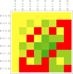
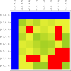
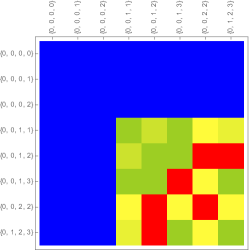
$\lambda=(2,1,1)$	$\lambda=(1,1,1,1)$	$\operatorname{Tr}\left[\hat{a}(\lambda)^{\dagger}\hat{a}(\lambda)\right]$

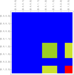
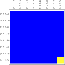
Figure 2: Symmetry-resolved transitions for $N=4$ particle in a Fourier interferometer with $M=4$ modes. The colour code gives $\operatorname{Tr}\left[\hat{a}(\lambda)^{\dagger}\hat{a}(\lambda)\right]$ for (inequivalent) pairs $\ket{\bm{i}}$ and $\ket{\bm{o}}$ of input and output state, for each symmetry type $\lambda$. Transitions to or from Pauli-forbidden states are marked in blue. Otherwise suppressed transitions are marked in red.

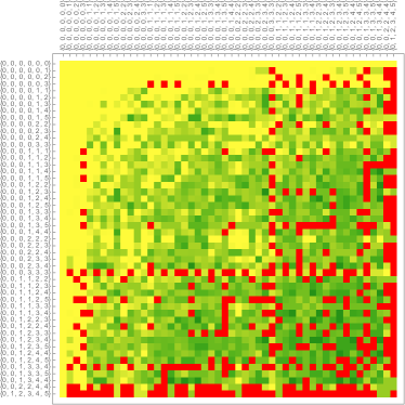
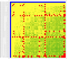
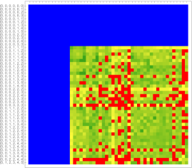
Figure 3: Symmetry-resolved transitions for $N=6$ particle in a Fourier interferometer with $M=6$ modes. The colour code gives $\operatorname{Tr}\left[\hat{a}(\lambda)^{\dagger}\hat{a}(\lambda)\right]$ for (inequivalent) pairs $\ket{\bm{i}}$ and $\ket{\bm{o}}$ of input and output states (x- and y-axes), for $\lambda=(6)$ (top), $\lambda=(5,1)$ (middle) and $\lambda=(3,3)$ (bottom). Transitions to or from Pauli-forbidden states are marked in blue. Otherwise suppressed transitions are marked in red.

In the following, it is convenient to label the modes modulo $M$, such that the $m$th mode, with $0\leq m\leq M-1$, is labelled by any integer of the form $m+kM$, $k\in\mathbb{Z}$. The cyclic group of order $M$ acts on the set of modes by translations $\Pi_{p}:\ket{m}\mapsto\ket{m+p},\,p\in\mathbb{Z}$, all of which are diagonalized by the Fourier unitary $U$. The cyclic group can be complemented by reflections $\Sigma_{p}:\ket{m}\mapsto\ket{p-m}$ (with $\Sigma_{p}=\Sigma_{p}^{-1}=\Sigma_{p}^{\dagger}$) to generate the dihedral group $D_{M}$: the symmetry group of a regular polygon whose vertices are identified with the modes.

The many-particle transition amplitude function for the Fourier unitary and input and output states $\ket{\bm{i}}$ and $\ket{\bm{o}}$ reads

$$a(\sigma)=M^{-N/2}\exp\left(\frac{2\mathrm{i}\pi}{M}\sum_{\alpha}o_{\alpha}i_{\sigma(\alpha)}\right)$$ (107)

and take values (up to the prefactor $M^{-N/2}$) in the set of $M$th roots of unity. It is therefore convenient to define

$$k(\sigma)=\frac{M}{2\mathrm{i}\pi}\log M^{N/2}a(\sigma)=\sum_{\alpha}o_{\alpha}i_{\sigma(\alpha)}\mod M$$ (108)

which encodes the phase of $a(\sigma)$.

Applying $\Pi_{p}$ to the input state $\ket{\bm{i}}$ amounts to replacing $i_{\alpha}$ by $i_{\alpha}+p$ in Eq. (108), such that $k(\sigma)$ receives an additional contribution $p\sum_{\alpha}o_{\alpha}\mod M$, corresponding to a rotation of $a(\sigma)$ in the complex plane. Furthermore, applying $\Sigma_{p}$ to the input state changes $k(\sigma)$ to $p\sum_{\alpha}o_{\alpha}-k(\sigma)\mod M$, amounting to a combined complex conjugation (i.e. reflection across the real axis) and rotation of $a(\sigma)$. The same holds for dihedral transformations of the output state. Applying an operation of the dihedral group $D_{M}$ to the input or output modes therefore results in a dihedral transformation of the distribution of many-particle transition amplitudes in the complex plane.

Such transformations are seen to leave $\operatorname{Tr}\left[\hat{a}(\lambda)^{\dagger}\hat{a}(\lambda)\right]$ unchanged. Moreover, exchanging input and output states maps $a(\sigma)$ to $a(\sigma^{-1})$, which also does not affect $\operatorname{Tr}\left[\hat{a}(\lambda)^{\dagger}\hat{a}(\lambda)\right]$. Recall also that this quantity is always invariant under independent permutations of the input and output particles. These symmetries mean that we can greatly reduce the number of distinct transition probabilities that need to be considered when searching for suppressed transitions.

Symmetry-induced suppressions occur when the distribution of the particles over the input and/or output modes is invariant under one of the operations of the dihedral group described above: a common translation $\Pi_{p}$ or a mirroring $\Sigma_{p}$ of the modes for all particles. In other word, up to a rearrangement of the particles by a permutation $\tau$, the input state $\ket{\bm{i}}$ (or output state $\ket{\bm{o}}$) is invariant under such a transformation. From the discussion above, we know that these symmetries of the states translate into symmetries of the distribution of transition amplitudes $a(\sigma)$ in the complex plane.

We identify three symmetries leading to suppressed transitions:

• Translational invariance of the input state: $\hat{R}(\tau)\ket{\bm{i}}=\Pi_{p}^{\otimes N}\ket{\bm{i}}$, such that $\delta_{\tau}*a=\Lambda a$ with $\Lambda=\exp\left(\frac{2\mathrm{i}\pi p}{M}\sum_{\alpha}o_{\alpha}\right)$.

• Translational invariance of the output state: $\hat{R}(\tau)\ket{\bm{o}}=\Pi_{p}^{\otimes N}\ket{\bm{o}}$, such that $a*\delta_{\tau}=\Lambda a$ with $\Lambda=\exp\left(\frac{2\mathrm{i}\pi p}{M}\sum_{\alpha}i_{\alpha}\right)$.

• Joint mirror symmetry of input and output states: $\hat{R}(\tau)\ket{\bm{i}}=\Sigma_{p}^{\otimes N}\ket{\bm{i}}$ and $\hat{R}(\tau^{\prime})\ket{\bm{o}}=\Sigma_{p^{\prime}}^{\otimes N}\ket{\bm{o}}$ , such that $\delta_{\tau}*a*\delta_{\tau^{\prime}}=\Lambda a$ with $\Lambda=\exp\left[\frac{2\mathrm{i}\pi}{M}\left(Npp^{\prime}-p\sum_{\alpha}o_{\alpha}-p^{\prime}\sum_{\alpha}i_{\alpha}\right)\right]$.

To illustrate suppressions due to translation invariance, we consider transitions from the following three input states with periodic occupations for a system of $N=6$ particles in $M=6$ modes:

• $\bm{i}=(0,1,2,3,4,5)$, such that $\hat{R}(\tau)\ket{\bm{i}}=\Pi_{p}^{\otimes N}\ket{\bm{i}}$ with $p=1$ and $\tau=(1\,2\,3\,4\,5\,6)$.

• $\bm{i}=(0,0,2,2,4,4)$, such that $\hat{R}(\tau)\ket{\bm{i}}=\Pi_{p}^{\otimes N}\ket{\bm{i}}$ with $p=2$ and $\tau=(1\,3\,6\,2\,4\,5)$.

• $\bm{i}=(0,0,1,3,3,4)$, such that $\hat{R}(\tau)\ket{\bm{i}}=\Pi_{p}^{\otimes N}\ket{\bm{i}}$ with $p=3$ and $\tau=(1\,4\,2\,5)(3\,6)$. Note that in this case, there is no cyclic permutation $\tau$ satisfying the above relation.

The corresponding values of $\operatorname{Tr}\left[\hat{a}(\lambda)^{\dagger}\hat{a}(\lambda)\right]$ for all inequivalent output states $\ket{\bm{o}}$ are shown in Fig. 4, with suppressed transitions marked in red. Notice the complementarity of suppressions between the bosonic and standard sectors in the first two cases, where a cyclic permutation $\tau$ exists. However, it can happen that both bosonic and standard transition amplitudes vanish, although one of them is in principle allowed, for example in the survival probability of the state with one particle per mode (last column in the top panel of Fig. 4). In this particular scenario, the suppressions are “inherited” from the $N=5$ case: for 5 indistinguishable bosons in distinct input modes of the $M=6$ Fourier interferometer, there are no allowed transitions to states with exactly one unoccupied output. Adding a sixth particle, whether it is distinguishable from the others or not, simply multiplies the — vanishing — 5-particle transition amplitudes by an extra factor.

$\bm{i}=(0,1,2,3,4,5)$

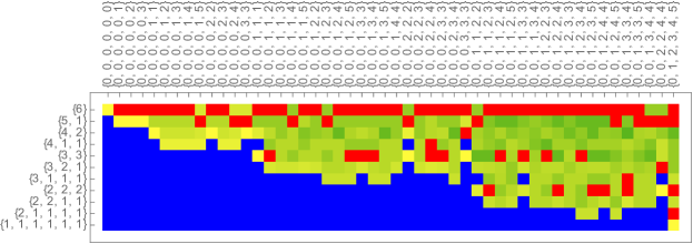
$\bm{i}=(0,0,2,2,4,4)$

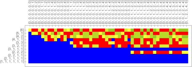
$\bm{i}=(0,0,1,3,3,4)$

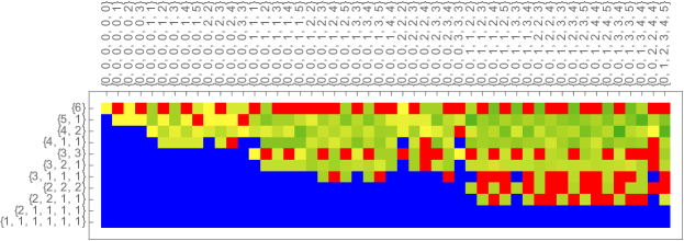
Figure 4: Transitions from three input configurations $\bm{i}$ with periodic occupations for a Fourier interferometer with $M=N=6$. The colour code gives the value of $\operatorname{Tr}\left[\hat{a}(\lambda)^{\dagger}\hat{a}(\lambda)\right]$ for (inequivalent) outputs $\bm{o}$ (x-axis), and irreps $\lambda$ (y-axis). Transitions to or from Pauli-forbidden states are marked in blue. Suppressed transitions are marked in red.

As an example of a suppression due to a joint mirror symmetries of input and output, consider again $N=M=6$. The input state with $\bm{i}=(0,0,0,1,3,5)$ satisfies $\hat{R}(\tau)\ket{\bm{i}}=\Sigma_{p}^{\otimes N}\ket{\bm{i}}$ with $p=0$ and $\tau=(4\,6)$. The output state with $\bm{o}=(0,0,1,2,3,3)$ satisfies $\hat{R}(\tau^{\prime})\ket{\bm{o}}=\Sigma_{p^{\prime}}^{\otimes N}\ket{\bm{o}}$ with $p^{\prime}=3$ and $\tau^{\prime}=(1\,6)(2\,5)(3\,4)$. We therefore have $\delta_{\tau}*a*\delta_{\tau^{\prime}}=\Lambda a$ with $\Lambda=-1$. Indeed, as shown in Fig. 5, the distribution of many-particle transition amplitudes is symmetric around the origin of the complex plane, leading to a suppression of the bosonic transition.

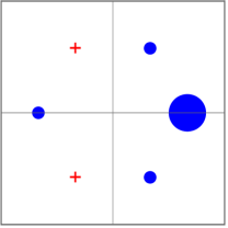
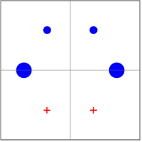
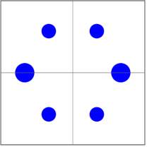
Figure 5: Left: Distribution of $N=6$ particles over $M=6$ modes, identified with the vertices of a hexagon, for the input mode list $\bm{i}=(0,0,0,1,3,5)$. Notice the mirror symmetry across the x-axis. Middle: same for the output mode list $\bm{o}=(0,0,1,2,3,3)$. Notice the symmetry across the y-axis. Right: Corresponding distribution of many-particle transition amplitudes $\{a(\sigma)=\braket{\bm{o}}{R(\sigma)^{\dagger}U^{\otimes N}}{\bm{i}}|\sigma\in S_{n})\}$ in the complex plane for the Fourier unitary. Notice the joint symmetry across the x- and y-axes, resulting in a symmetry around the origin. The radius of the blue dots is proportional to the number of particles or amplitudes.

Pauli-like suppressions arise from the invariance of the transition amplitude function under a subgroup of $S_{N}$. In the extreme case of a constant function $a(\sigma)=a$, it is clear that $\hat{a}(\lambda)$ must vanish for all but the bosonic irrep. This can for example happen when particles only occupy equally separated input and output modes. Specifically, if particles on input only occupy modes $i$ that are a multiple of $p_{i}\in\mathbb{Z}$ while particles on output only occupy modes $o$ that are a multiple of $p_{o}\in\mathbb{Z}$, and if these periods satisfy $p_{i}p_{o}=0\mod M$, then it follows that for all $\sigma$, $k(\sigma)=0$, such that $a(\sigma)$ is constant.

Now if a single output particle, say the $N$th one, populates a mode $o$ which is not a multiple of $p_{o}$, then $k(\sigma)=oi_{\sigma(N)}\mod M$ depends only on $\sigma(N)$, and is therefore invariant under transformations of $S_{N-1}$. It follows that the transition is suppressed in all but the bosonic and standard sectors. Note that in this case, since $\sigma(N)$ takes each of the values $1,\dots N$ equally many times when $\sigma$ runs over $S_{N}$, the bosonic transition amplitude takes the simple form

$$\hat{a}(N)=M^{-N/2}(N-1)!\sum_{\alpha=1}^{N}\exp\left(\frac{2\mathrm{i}\pi}{M}oi_{\alpha}\right)=M^{-N/2}(N-1)!\sum_{m=0}^{M-1}n_{m}\exp\left(\frac{2\mathrm{i}\pi}{M}om\right),$$ (109)

where $n_{m}$ is the initial occupation of mode $m$. We recognise the $o_{N}$th component of the discrete Fourier transform of the initial particle distribution. If this vanishes, then the standard irrep is the only one in which the transition is not suppressed. Figure 6 shows an example of such a transition.

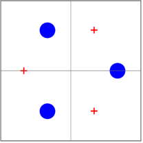
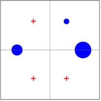
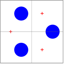
Figure 6: Left: Distribution of $N=6$ particles over $M=6$ modes, identified with the vertices of a hexagon, for the input mode list $\bm{i}=(0,0,2,2,4,4)$. Occupied modes are all multiples of $p_{i}=2$. Middle: same for the output mode list $\bm{o}=(0,0,0,1,3,3)$. A single particle occupies a mode ($o=1$) which is not a multiple of $p_{o}=3$. As a consequence, for the Fourier unitary, there is a Pauli-like suppression in all sectors apart from the bosonic and standard ones. Because of the input state’s periodicity, the bosonic transition is symmetry-suppressed, such that only the standard sector is not suppressed. Right: Corresponding distribution of many-particle transition amplitudes $\{a(\sigma)=\braket{\bm{o}}{R(\sigma)^{\dagger}U^{\otimes N}}{\bm{i}}|\sigma\in S_{n})\}$ in the complex plane. The three-fold rotation symmetry reflects that of the input state.

When more particles do not populate equally spaced sites, the subgroup of permutations fixing $a(\sigma)$ becomes smaller, implying Pauli-like suppressions in fewer symmetry sectors and a more complex expression for the bosonic transition amplitude. For example, if $k$ output particles all populate a mode $o$ which is not a multiple of $p_{o}$, the bosonic transition amplitude is proportional to

$$\hat{a}(N)\propto\sum_{\alpha_{1}<\alpha_{2}\dots<\alpha_{k}}\exp\left(\frac{2\mathrm{i}\pi}{M}o\sum_{j=1}^{k}i_{\alpha_{j}}\right),$$ (110)

which, for moderate $k$, can reasonably easily be seen to vanish or not, depending on $\bm{i}$.

VI Conclusion

We have introduced the powerful tools of Fourier analysis to the study of many-body interference in the dynamics of identical particles. In particular, we investigated the Fourier transforms of the many-particle transition amplitude function $a$ — which gathers all possible transition amplitudes between the initial and final states of $N$ particles — and of the partial distinguishability function $j$ — which encodes effects due to internal states of the particles. The non-commutativity of the group of particle permutations results in a rich structure of the Fourier transforms, with matrix-valued mixed-symmetry components alongside the single-dimensional bosonic and fermionic components. We have argued that this decomposition into exchange symmetry sectors provides a natural framework to understand the effect of partial distinguishability in the interference of systems of bosons or fermions.

We already see several opportunities of applying the present framework to further problems in the fields of many-body physics, quantum optics and quantum information.

Since it relies only on the commutation of the evolution operator with particle permutations, and not on its factorization as a product of single-particle unitaries, our symmetry-based approach offers a promising way of including interaction effects to many-particle interference scenarios [31, 62, 63, 33] beyond the perturbative regime [64].

Although we haven’t addressed this possibility explicitly, we also believe that the present framework is useful to describe many-body systems which do not have an intrinsic exchange symmetry (e.g. spin chains or qubit registers), but which are submitted to symmetric evolution and measurement protocols, rendering them “operationally indistinguishable” [65]. In this context, entangled states with mixed symmetries would benefit from protection against global noise.

Bosonic suppression laws generalizing the Hong-Ou-Mandel effect have recently been applied to the generation of entangled states [66, 67] and to the distillation of pure and indistinguishable photons [68, 69]. We are confident that our investigation of completely destructive interference beyond the bosonic and fermionic symmetry sectors will allow to optimize such protocols, or to tune them towards the generation of states with a specific symmetry $\lambda$.

Finally, our discussion of suppressed transitions in the Fourier interferometer has uncovered an interesting interplay between the Fourier transforms over the permutation group of the particles ($S_{N}$) on the one hand and the translation group of the modes ($\mathbb{Z}/M\mathbb{Z}$) on the other, whose full consequences remain to be elucidated.

Appendices

Appendix A Fourier inversion formula

We give a brief justification for the Fourier inversion formula, Eq. (6). It can be understood in light of the Grand Orthogonality Theorem: for matrix irreps $\rho^{(\lambda)}$, $\rho^{(\nu)}$ of a finite group $G$, it holds [46, 47, 48]

$$\sum_{\sigma\in G}\hat{\rho}_{mn}^{(\lambda)}(\sigma^{-1})\hat{\rho}_{n^{\prime}m^{\prime}}^{(\mu)}(\sigma)=\frac{|G|}{d_{\lambda}}\delta_{\lambda\mu}\delta_{mm^{\prime}}\delta_{nn^{\prime}}.$$ (111)

In essence, the above relation means that the individual entries of the matrix irreps form an orthogonal set of functions from $G$ to $\mathbb{C}$. Since $\sum_{\lambda}d_{\lambda}^{2}=|G|$, this set forms a basis, and Eq. (6) is the expansion of $f$ in that basis.

Setting $n=m$ and $n^{\prime}=m^{\prime}$ in Eq. (111) and summing over $m$ and $m^{\prime}$, we obtain the following relation for the irreducible characters $\chi^{(\lambda)}(\sigma)=\operatorname{Tr}(\hat{\rho}^{(\lambda)}(\sigma))$:

$$\sum_{\sigma\in G}\chi^{(\lambda)}(\sigma^{-1})\chi^{(\mu)}(\sigma)=|G|\delta_{\lambda\mu}.$$ (112)

Viewing the above as an orthogonality relation for the rows of the character table, we can deduce the following orthogonality relation for its columns:

$$\sum_{\lambda}\chi^{(\lambda)}(\sigma^{-1})\chi^{(\lambda)}(\tau)=\begin{cases}|G|/|C|&\text{ if }\sigma\text{ and }\tau\text{ are in the same conjugacy class }C,\\ 0&\text{ otherwise.}\end{cases}$$ (113)

In particular, given that the group’s identity element $\operatorname{id}$ is alone in its conjugacy class and that $\chi^{(\lambda)}(\operatorname{id})=d_{\lambda}$, we have

$$\sum_{\lambda}\frac{d_{\lambda}}{|G|}\chi^{(\lambda)}(\tau)=\delta_{\tau,\operatorname{id}}.$$ (114)

The proof of Eq. (6) follows after replacing $\hat{f}(\lambda)$ by its definition [Eq. (4)] and applying the above relation.

Appendix B Formulas for counting statistics

We provide proofs of the formulas Eq. (66) and Eq. (78).

Equation (66) gives the counting statistics arising from an initial state $\hat{c}\ket{\bm{i}}$:

$$P_{\{n_{m}\}} =\frac{\braket{\bm{i}}{\hat{c}^{\dagger}U^{\dagger\otimes N}P_{\bm{o}}U^{\otimes N}\hat{c}}{\bm{i}}}{\braket{\bm{i}}{\hat{c}^{\dagger}\hat{c}}{\bm{i}}}.$$ (115)

By definition of the projector $P_{\bm{o}}$ [Eq. (64)], the numerator reads

$$\braket{\bm{i}}{\hat{c}^{\dagger}U^{\dagger\otimes N}P_{\bm{o}}U^{\otimes N}\hat{c}}{\bm{i}} =\frac{1}{|\operatorname{stab}(\bm{o})|}\sum_{\sigma\in S_{N}}\braket{\bm{i}}{\hat{c}^{\dagger}U^{\dagger\otimes N}\hat{R}(\sigma)\ket{\bm{o}}\bra{\bm{o}}\hat{R}(\sigma)^{\dagger}U^{\otimes N}\hat{c}}{\bm{i}}.$$ (116)

Recognising

$$\braket{\bm{o}}{\hat{R}(\sigma)^{\dagger}U^{\otimes N}\hat{c}}{\bm{i}}=(c*a)(\sigma),$$ (117)

we thus have

$$\braket{\bm{i}}{\hat{c}^{\dagger}U^{\dagger\otimes N}P_{\bm{o}}U^{\otimes N}\hat{c}}{\bm{i}} =\frac{1}{|\operatorname{stab}(\bm{o})|}((c*a)^{\star},c*a)$$ (118)

and by the Parseval-Plancherel identity,

$$\braket{\bm{i}}{\hat{c}^{\dagger}U^{\dagger\otimes N}P_{\bm{o}}U^{\otimes N}\hat{c}}{\bm{i}} =\frac{1}{|\operatorname{stab}(\bm{o})|}\sum_{\lambda}\frac{d_{\lambda}}{N!}\operatorname{Tr}\left[\hat{a}^{\dagger}(\lambda)\hat{c}^{\dagger}(\lambda)\hat{c}(\lambda)\hat{a}(\lambda)\right].$$ (119)

The denominator evaluates to

$$\braket{\bm{i}}{\hat{c}^{\dagger}\hat{c}}{\bm{i}}=\braket{\bm{i}}{\widehat{c^{\star}*c}}{\bm{i}}=|\operatorname{stab}(\bm{i})|(I_{\bm{i}},c^{\star}*c)=|\operatorname{stab}(\bm{i})|\sum_{\lambda}\frac{d_{\lambda}}{N!}\operatorname{Tr}\left[\hat{I}_{\bm{i}}(\lambda)\hat{c}^{\dagger}(\lambda)\hat{c}(\lambda)\right],$$ (120)

such that

$$P_{\{n_{m}\}} =\frac{1}{|\operatorname{stab}(\bm{i})||\operatorname{stab}(\bm{o})|}\frac{\sum_{\lambda}d_{\lambda}\operatorname{Tr}\left[\hat{a}^{\dagger}(\lambda)\hat{c}^{\dagger}(\lambda)\hat{c}(\lambda)\hat{a}(\lambda)\right]}{\sum_{\lambda}d_{\lambda}\operatorname{Tr}\left[\hat{I}_{\bm{i}}(\lambda)\hat{c}^{\dagger}(\lambda)\hat{c}(\lambda)\right]}.$$ (121)

Equation (78) gives the same probability in the case of partially distinguishable particles with initial external state $\varrho$:

$$P_{\{n_{m}\}}=\operatorname{Tr}(U^{\otimes N}\varrho U^{\dagger\otimes N}P_{\bm{o}}).$$ (122)

We assume that $\varrho$ is supported on the subspace generated by vectors $\hat{R}(\sigma)\ket{\bm{i}}$ for $\sigma\in S_{N}$. The projector on this subspace reads

$$P_{\bm{i}}=\frac{1}{|\operatorname{stab}(\bm{i})|}\sum_{\sigma\in S_{N}}\hat{R}(\sigma)\ket{\bm{i}}\bra{\bm{i}}\hat{R}(\sigma)^{\dagger},$$ (123)

in analogy with the projector $P_{\bm{o}}$ of Eq. (64). We can thus write

$$P_{\{n_{m}\}} =\frac{1}{|\operatorname{stab}(\bm{o})||\operatorname{stab}(\bm{i})|^{2}}\sum_{\sigma,\tau,\pi\in S_{N}}\braket{\bm{o}}{\hat{R}(\sigma)^{\dagger}U^{\otimes N}\hat{R}(\tau)}{\bm{i}}\braket{\bm{i}}{\hat{R}(\tau)^{\dagger}\varrho\hat{R}(\pi)}{\bm{i}}\braket{\bm{i}}{\hat{R}(\pi)^{\dagger}U^{\dagger\otimes N}\hat{R}(\sigma)}{\bm{o}}$$ (124)

$$=\frac{1}{N!|\operatorname{stab}(\bm{o})||\operatorname{stab}(\bm{i})|}\sum_{\sigma,\tau,\pi\in S_{N}}a(\tau^{-1}\circ\sigma)j(\pi^{-1}\circ\tau)a(\pi^{-1}\circ\sigma)^{*}$$ (125)

$$=\frac{1}{N!|\operatorname{stab}(\bm{o})||\operatorname{stab}(\bm{i})|}\sum_{\sigma,\pi\in S_{N}}a^{\star}(\sigma^{-1}\circ\pi)(j*a)(\pi^{-1}\circ\sigma)$$ (126)

$$=\frac{1}{|\operatorname{stab}(\bm{o})||\operatorname{stab}(\bm{i})|}(a^{\star},j*a).$$ (127)

Finally, with the Parseval-Plancherel identity,

$$P_{\{n_{m}\}}=\frac{1}{|\operatorname{stab}(\bm{o})||\operatorname{stab}(\bm{i})|}\sum_{\lambda}\frac{d_{\lambda}}{N!}\operatorname{Tr}\left[\hat{a}^{\dagger}(\lambda)\hat{j}(\lambda)\hat{a}(\lambda)\right].$$ (128)

Appendix C Sector weights and purity of states of partially distinguishable particles

We prove equations (79) and (80).

The weight of a state $\varrho$ on symmetry sector $\lambda$ is given by $p_{\lambda}=\operatorname{Tr}\left[\varrho\hat{P}^{(\lambda)}\right]$. With the definition (19) of the isotypic projector and since $\varrho=P_{\bm{i}}\varrho$, with $P_{\bm{i}}$ from Eq. (123), we have

$$p_{\lambda} =\operatorname{Tr}\left[\varrho\hat{P}^{(\lambda)}\right]$$ (129)

$$=\frac{1}{|\operatorname{stab}(\bm{i})|}\frac{d_{\lambda}}{N!}\sum_{\sigma,\tau\in S_{N}}\chi^{(\lambda)}(\sigma)\braket{\bm{i}}{\hat{R}(\tau)^{\dagger}\varrho\hat{R}(\sigma)\hat{R}(\tau)}{\bm{i}}$$ (130)

$$=\frac{d_{\lambda}}{(N!)^{2}}\sum_{\sigma,\tau\in S_{N}}\chi^{(\lambda)}(\sigma)j(\tau^{-1}\circ\sigma^{-1}\circ\tau).$$ (131)

Changing variables from $\sigma$ to $\pi=\tau^{-1}\circ\sigma^{-1}\circ\tau$, we obtain

$$p_{\lambda} =\frac{d_{\lambda}}{(N!)^{2}}\sum_{\pi,\tau\in S_{N}}\chi^{(\lambda)}(\tau\circ\pi^{-1}\circ\tau^{-1})j(\pi)$$ (132)

$$=\frac{d_{\lambda}}{N!}\sum_{\pi\in S_{N}}\chi^{(\lambda)}(\pi^{-1})j(\pi),$$ (133)

since $\chi^{(\lambda)}$ is a class function. Writing the scalar product $(\chi^{(\lambda)},j)$ in terms of Fourier transforms, we conclude that

$$p_{\lambda} =\frac{d_{\lambda}}{N!}\operatorname{Tr}[\hat{j}(\lambda)].$$ (134)

The expression (80) for the purity of $\varrho$ is readily obtained using the representation (77) of $\varrho$ in terms of $j$. We have

$$\operatorname{Tr}\left[\varrho^{2}\right]=\frac{1}{(N!)^{2}}\sum_{\sigma,\tau\in S_{N}}\sum_{\sigma^{\prime},\tau^{\prime}\in S_{N}}j(\tau^{-1}\circ\sigma)j(\tau^{\prime-1}\circ\sigma^{\prime})I_{\bm{i}}(\sigma^{-1}\circ\tau^{\prime})I_{\bm{i}}(\sigma^{\prime-1}\circ\tau).$$ (135)

Noting that $j*I_{\bm{i}}=I_{\bm{i}}*j=j$, we obtain

$$\operatorname{Tr}\left[\varrho^{2}\right] =\frac{1}{(N!)^{2}}\sum_{\sigma,\sigma^{\prime}\in S_{N}}j(\sigma^{\prime-1}\circ\sigma)j(\sigma^{-1}\circ\sigma^{\prime})$$ (136)

$$=\frac{1}{N!}(j,j)$$ (137)

$$=\frac{1}{N!}\sum_{\lambda}\frac{d_{\lambda}}{N!}\operatorname{Tr}\left[\hat{j}(\lambda)^{2}\right].$$ (138)

Appendix D Positivity of $\hat{j}$

We show that the Fourier transform $\hat{j}(\rho)$ of $j$ at any unitary representation $\rho$ of dimension $d$ is positive, i.e. for any vector $\vec{x}\in\mathbb{C}^{d}$, $\vec{x}^{\dagger}\hat{j}(\rho)\vec{x}\geq 0$.

We have

$$\vec{x}^{\dagger}\hat{j}(\rho)\vec{x} =\sum_{\sigma\in S_{N}}j(\sigma)\ \vec{x}^{\dagger}\hat{\rho}(\sigma)\vec{x}=\frac{1}{N!}\sum_{\sigma,\tau\in S_{N}}j(\tau^{-1}\circ\sigma)\ \vec{x}^{\dagger}\hat{\rho}(\tau^{-1}\circ\sigma)\vec{x}.$$ (139)

Given that

$$j(\tau^{-1}\circ\sigma)=\frac{N!}{|\operatorname{stab}(\bm{i})|}\braket{\bm{i}}{\hat{R}(\tau^{-1}\circ\sigma)^{\dagger}\varrho}{\bm{i}}=\frac{N!}{|\operatorname{stab}(\bm{i})|}\braket{\bm{i}}{\hat{R}(\sigma)^{\dagger}\varrho\hat{R}(\tau)}{\bm{i}}$$ (140)

and

$$\hat{\rho}(\tau^{-1}\circ\sigma)=\hat{\rho}(\tau)^{\dagger}\hat{\rho}(\sigma),$$ (141)

we can write

$$\vec{x}^{\dagger}\hat{j}(\rho)\vec{x} =\frac{1}{|\operatorname{stab}(\bm{i})|}\sum_{\sigma,\tau\in S_{N}}\braket{\bm{i}}{\hat{R}(\sigma)^{\dagger}\varrho\hat{R}(\tau)}{\bm{i}}\vec{x}^{\dagger}\hat{\rho}(\tau)^{\dagger}\hat{\rho}(\sigma)\vec{x}$$ (142)

$$=\frac{1}{|\operatorname{stab}(\bm{i})|}\sum_{\sigma,\tau\in S_{N}}\braket{\bm{i}}{\hat{R}(\sigma)^{\dagger}\varrho\hat{R}(\tau)}{\bm{i}}\vec{y}(\tau)^{\dagger}\vec{y}(\sigma).$$ (143)

where we have defined the vector valued function $\vec{y}(\sigma)=\hat{\rho}(\sigma)\vec{x}$. Decomposing it into components, we find

$$\vec{x}^{\dagger}\hat{j}(\rho)\vec{x}=\frac{1}{|\operatorname{stab}(\bm{i})|}\sum_{\sigma,\tau\in S_{N}}\sum_{k=1}^{d}\braket{\bm{i}}{\hat{R}(\sigma)^{\dagger}y_{k}(\sigma)\varrho y_{k}(\tau)^{*}\hat{R}(\tau)}{\bm{i}}=\frac{1}{|\operatorname{stab}(\bm{i})|}\sum_{k=1}^{d}\braket{\psi_{k}}{\varrho}{\psi_{k}},$$ (144)

with

$$\ket{\psi_{k}}=\sum_{\tau\in S_{N}}y_{k}(\tau)^{*}\hat{R}(\tau)\ket{\bm{i}}.$$ (145)

By positivity of $\varrho$, every term in the right-hand side of Eq. (144) is positive and we conclude that $\vec{x}^{\dagger}\hat{j}(\rho)\vec{x}\geq 0$.

References

- Diaconis [1988] P. Diaconis, in École d’Été de Probabilités de Saint-Flour XV–XVII, 1985–87, Vol. 1362 (Springer Berlin Heidelberg, Berlin, Heidelberg, 1988) pp. 51–100.
- Rockmore [1997] D. N. Rockmore, DIMACS Series in Discrete Mathematics and Theoretical Computer Science (1997).
- Diaconis [1989] P. Diaconis, The Annals of Statistics , 949 (1989), 2241705 .
- Daugherty et al. [2007] Z. Daugherty, A. K. Eustis, G. Minton, and M. E. Orrison, Voting, the symmetric group, and representation theory (2007), arXiv:0712.2837 [math] .
- Terras [1999] A. Terras, Fourier Analysis on Finite Groups and Applications, London Mathematical Society Student Texts (Cambridge University Press, Cambridge, 1999).
- Kondor [2008] I. R. Kondor, Group Theoretical Methods in Machine Learning (Columbia University, 2008).
- Cooley and Tukey [1965] J. W. Cooley and J. W. Tukey, Mathematics of Computation 19, 297 (1965).
- Clausen [1989] M. Clausen, Theoretical Computer Science 67, 55 (1989).
- Diaconis and Rockmore [1990] P. Diaconis and D. Rockmore, Journal of the American Mathematical Society 3, 297 (1990).
- Shchesnovich [2015a] V. S. Shchesnovich, Physical Review A 91, 013844 (2015a).
- Tichy [2015] M. C. Tichy, Physical Review A 91, 022316 (2015).
- Dittel et al. [2021] C. Dittel, G. Dufour, G. Weihs, and A. Buchleitner, Physical Review X 11, 031041 (2021).
- Walschaers et al. [2016] M. Walschaers, J. Kuipers, J.-D. Urbina, K. Mayer, M. C. Tichy, Klaus Richter, and A. Buchleitner, New Journal of Physics 18, 032001 (2016).
- Giordani et al. [2018] T. Giordani, F. Flamini, M. Pompili, N. Viggianiello, N. Spagnolo, A. Crespi, R. Osellame, N. Wiebe, M. Walschaers, A. Buchleitner, and F. Sciarrino, Nature Photonics 12, 173 (2018).
- Stanisic and Turner [2018] S. Stanisic and P. S. Turner, Physical Review A 98, 043839 (2018).
- Giordani et al. [2020] T. Giordani, D. J. Brod, C. Esposito, N. Viggianiello, M. Romano, F. Flamini, G. Carvacho, N. Spagnolo, E. F. Galvão, and F. Sciarrino, New Journal of Physics 22, 043001 (2020).
- Brunner et al. [2022] E. Brunner, A. Buchleitner, and G. Dufour, Physical Review Research 4, 043101 (2022).
- Tan et al. [2013] S.-H. Tan, Y. Y. Gao, H. de Guise, and B. C. Sanders, Physical Review Letters 110, 113603 (2013).
- de Guise et al. [2014] H. de Guise, S.-H. Tan, I. P. Poulin, and B. C. Sanders, Physical Review A 89, 063819 (2014).
- Tillmann et al. [2015] M. Tillmann, S.-H. Tan, S. E. Stoeckl, B. C. Sanders, H. de Guise, R. Heilmann, S. Nolte, A. Szameit, and P. Walther, Physical Review X 5, 041015 (2015).
- Menssen et al. [2017] A. J. Menssen, A. E. Jones, B. J. Metcalf, M. C. Tichy, S. Barz, W. S. Kolthammer, and I. A. Walmsley, Physical Review Letters 118, 153603 (2017).
- Jones et al. [2020] A. E. Jones, A. J. Menssen, H. M. Chrzanowski, T. A. W. Wolterink, V. S. Shchesnovich, and I. A. Walmsley, Physical Review Letters 125, 123603 (2020).
- Seron et al. [2023] B. Seron, L. Novo, and N. J. Cerf, Nature Photonics 17, 702 (2023).
- Weyl [1950] H. Weyl, The Theory of Groups and Quantum Mechanics (Courier Corporation, 1950).
- Wigner [1959] E. Wigner, Group Theory and Its Application to the Quantum Mechanics of Atomic Spectra. (New York: Academic Press., 1959).
- Adamson et al. [2007] R. B. A. Adamson, L. K. Shalm, M. W. Mitchell, and A. M. Steinberg, Physical Review Letters 98, 043601 (2007).
- Adamson et al. [2008] R. B. A. Adamson, P. S. Turner, M. W. Mitchell, and A. M. Steinberg, Physical Review A 78, 033832 (2008).
- Rowe et al. [2012] D. J. Rowe, M. J. Carvalho, and J. Repka, Reviews of Modern Physics 84, 711 (2012).
- Moylett and Turner [2018] A. E. Moylett and P. S. Turner, Physical Review A 97, 062329 (2018).
- Khalid et al. [2018] A. Khalid, D. Spivak, B. C. Sanders, and H. de Guise, Physical Review A 97, 063802 (2018).
- Dufour et al. [2020] G. Dufour, T. Brünner, A. Rodríguez, and A. Buchleitner, New Journal of Physics 22, 103006 (2020).
- Spivak et al. [2022] D. Spivak, M. Y. Niu, B. C. Sanders, and H. de Guise, Physical Review Research 4, 023013 (2022).
- Brunner et al. [2023] E. Brunner, L. Pausch, E. G. Carnio, G. Dufour, A. Rodríguez, and A. Buchleitner, Physical Review Letters 130, 080401 (2023).
- Note [1] We use the Young Orthogonal representation as implemented in H. Pan’s SnPy package github.com/horacepan/snpy.
- Messiah and Greenberg [1964] A. M. L. Messiah and O. W. Greenberg, Physical Review 136, B248 (1964).
- Tichy and Mølmer [2017] M. C. Tichy and K. Mølmer, Physical Review A 96, 022119 (2017).
- Lim and Beige [2005] Y. L. Lim and A. Beige, New Journal of Physics 7, 155 (2005).
- Tichy et al. [2010] M. C. Tichy, M. Tiersch, F. de Melo, F. Mintert, and A. Buchleitner, Physical Review Letters 104, 220405 (2010).
- Tichy et al. [2012] M. C. Tichy, M. Tiersch, F. Mintert, and A. Buchleitner, New Journal of Physics 14, 093015 (2012).
- Tichy et al. [2014] M. C. Tichy, K. Mayer, A. Buchleitner, and K. Mølmer, Physical Review Letters 113, 020502 (2014).
- Crespi [2015] A. Crespi, Physical Review A 91, 013811 (2015).
- Crespi et al. [2016] A. Crespi, R. Osellame, R. Ramponi, M. Bentivegna, F. Flamini, N. Spagnolo, N. Viggianiello, L. Innocenti, P. Mataloni, and F. Sciarrino, Nature Communications 7, 10469 (2016).
- Dittel et al. [2017] C. Dittel, R. Keil, and G. Weihs, Quantum Science and Technology 2, 015003 (2017).
- Dittel et al. [2018a] C. Dittel, G. Dufour, M. Walschaers, G. Weihs, A. Buchleitner, and R. Keil, Physical Review Letters 120, 240404 (2018a).
- Dittel et al. [2018b] C. Dittel, G. Dufour, M. Walschaers, G. Weihs, A. Buchleitner, and R. Keil, Physical Review A 97, 062116 (2018b).
- Hamermesh [1989] M. Hamermesh, Group Theory and Its Application to Physical Problems (Courier Corporation, 1989).
- Chen et al. [2002] J.-q. Chen, J. Ping, and F. Wang, Group Representation Theory For Physicists (2nd Edition) (World Scientific Publishing Company, 2002).
- Sengupta [2011] A. N. Sengupta, Representing Finite Groups: A Semisimple Introduction (Springer Science & Business Media, 2011).
- Hartle and Taylor [1969] J. B. Hartle and J. R. Taylor, Physical Review 178, 2043 (1969).
- Stolt and Taylor [1970] R. H. Stolt and J. R. Taylor, Nuclear Physics B 19, 1 (1970).
- Note [2] Gamas’ theorem states that for (not necessarily orthogonal) single-particle states , is non vanishing if and only if the can be partitioned into linearly independent sets whose sizes are given by the lengths of the columns of the Young diagram .
- Gamas [1988] C. Gamas, Linear Algebra and its Applications 108, 83 (1988).
- Pate [1990] T. H. Pate, Linear and Multilinear Algebra 28, 175 (1990).
- Berget [2009] A. Berget, Linear Algebra and its Applications 430, 791 (2009).
- Shchesnovich [2015b] V. S. Shchesnovich, Physical Review A 91, 063842 (2015b).
- Englbrecht et al. [2024] M. Englbrecht, T. Kraft, C. Dittel, A. Buchleitner, G. Giedke, and B. Kraus, Physical Review Letters 132, 050201 (2024).
- Shchesnovich [2014] V. S. Shchesnovich, Physical Review A 89, 022333 (2014).
- Shchesnovich [2016] V. S. Shchesnovich, Physical Review Letters 116, 123601 (2016).
- Hong et al. [1987] C. K. Hong, Z. Y. Ou, and L. Mandel, Physical Review Letters 59, 2044 (1987).
- Bouchard et al. [2021] F. Bouchard, A. Sit, Y. Zhang, R. Fickler, F. M. Miatto, Y. Yao, F. Sciarrino, and E. Karimi, Reports on Progress in Physics 84, 012402 (2021).
- Bezerra and Shchesnovich [2023] M. E. O. Bezerra and V. S. Shchesnovich, New Journal of Physics 25, 093047 (2023).
- Bressanini et al. [2022] G. Bressanini, H. Kwon, and M. S. Kim, Physical Review A 106, 042413 (2022).
- Spagnolo et al. [2023] N. Spagnolo, D. J. Brod, E. F. Galvão, and F. Sciarrino, npj Quantum Information 9, 1 (2023).
- Brünner et al. [2018] T. Brünner, G. Dufour, A. Rodríguez, and A. Buchleitner, Physical Review Letters 120, 210401 (2018).
- Yadin et al. [2023] B. Yadin, B. Morris, and K. Brandner, Physical Review Research 5, 033018 (2023).
- Bhatti and Barz [2023] D. Bhatti and S. Barz, Physical Review A 107, 033714 (2023).
- Piccolini et al. [2024] M. Piccolini, M. Karczewski, A. Winter, and R. L. Franco, Robust generation of $N$-partite $N$-level singlet states by identical particle interferometry (2024), arXiv:2312.17184 [quant-ph] .
- Somhorst et al. [2024] F. H. B. Somhorst, B. K. Sauër, S. N. van den Hoven, and J. J. Renema, Photon distillation schemes with reduced resource costs based on multiphoton Fourier interference (2024), arXiv:2404.14262 [quant-ph] .
- Saied et al. [2024] J. Saied, J. Marshall, N. Anand, and E. G. Rieffel, General protocols for the efficient distillation of indistinguishable photons (2024), arXiv:2404.14217 [physics, physics:quant-ph] .