Multivariate change estimation for a stochastic heat equation from local measurements

Abstract

We study a stochastic heat equation with piecewise constant diffusivity $\vartheta$ having a jump at a hypersurface $\Gamma$ that splits the underlying space $[0,1]^{d}$, $d\geq 2,$ into two disjoint sets $\Lambda_{-}\cup\Lambda_{+}.$ Based on multiple spatially localized measurement observations on a regular $\delta$-grid of $[0,1]^{d}$, we propose a joint M-estimator for the diffusivity values and the set $\Lambda_{+}$ that is inspired by statistical image reconstruction methods. We study convergence of the domain estimator $\widehat{\Lambda}_{+}$ in the vanishing resolution level regime $\delta\to 0$ and with respect to the expected symmetric difference pseudometric. Our main finding is a characterization of the convergence rate for $\widehat{\Lambda}_{+}$ in terms of the complexity of $\Gamma$ measured by the number of intersecting hypercubes from the regular $\delta$-grid. Implications of our general result are discussed under two specific structural assumptions on $\Lambda_{+}$. For a $\beta$-Hölder smooth boundary fragment $\Gamma$, the set $\Lambda_{+}$ is estimated with rate $\delta^{\beta}$. If we assume $\Lambda_{+}$ to be convex, we obtain a $\delta$-rate. While our approach only aims at optimal domain estimation rates, we also demonstrate consistency of our diffusivity estimators.

1 Introduction

Over the last decades interest in statistics for stochastic partial differential equations (SPDEs) has continuously increased for several reasons. Not only is it advantageous to model many natural space-time phenomena by SPDEs as they automatically account for model uncertainty by including random forcing terms that describe a more accurate picture of data dynamics, but also the general surge in data volume combined with enlarged computational power of modern computers makes it more appealing to investigate statistical problems for SPDEs.

In this paper we study a multivariate change estimation model for a stochastic heat equation on $\Lambda=(0,1)^{d},$ $d\geq 2,$ given by

$$\mathop{}\!\mathrm{d}X(t)=\Delta_{\vartheta}X(t)\mathop{}\!\mathrm{d}t+\mathop{}\!\mathrm{d}W(t),\quad 0\leq t\leq T,$$ (1.1)

with discontinuous diffusivity $\vartheta.$ The driving force is space-time white noise $\dot{W}(t)$ and the weighted Laplace operator $\Delta_{\vartheta}=\nabla\cdot\vartheta\nabla$ is characterized by a jump in the diffusivity

$$\vartheta(x)=\vartheta_{-}\mathbf{1}_{\Lambda_{-}}(x)+\vartheta_{+}\mathbf{1}_{\Lambda_{+}}(x),\quad x\in(0,1)^{d},$$ (1.2)

where the sets $\Lambda_{\pm}$ form a partition of $\overline{\Lambda}=[0,1]^{d}.$ Our primary interest lies in the construction of a nonparametric estimator of the change domain $\Lambda_{+}$, which is equivalently characterized by the hypersurface

$$\Gamma\coloneq\partial\Lambda_{-}\cap\partial\Lambda_{+}\subset[0,1]^{d}.$$ (1.3)

The SPDE (1.1) can, for instance, be used to describe the heat flow through two distinct materials with different heat conductivity, colliding in $\Gamma$. An exemplary illustration of the solution $X$ to (1.1) with $\Gamma=\{(x,y):y=x,0\leq x,y\leq 1\}$ in two spatial dimensions is given in Figure 1.1.

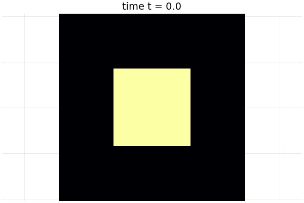
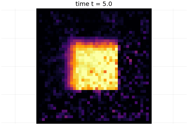
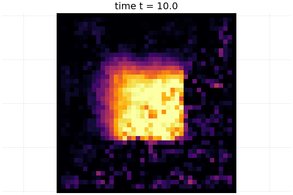
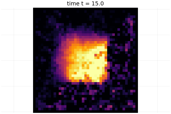
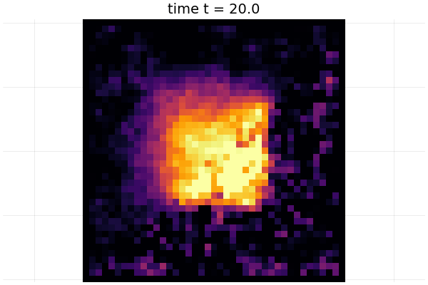
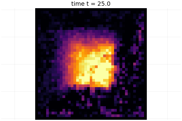
Figure 1.1: Realization of the solution $X$ to $\eqref{eq: intro SPDE}$ in $d=2$ with change curve $\Gamma=\{(x,y):y=x,0\leq x,y\leq 1\}$ at increasing time points.

Structurally, the statistical problem of estimating $\Gamma$ is closely related to image reconstruction problems where one usually considers a regression model with (possibly random) design points $X_{k}$ and observational noise $\varepsilon_{k}$ given by

$$Y_{k}=f(X_{k})+\varepsilon_{k},\quad 1\leq k\leq N,$$

where the $Y_{k}$ correspond to the observed color of a pixel centred around the spatial point $X_{k}\in[0,1]^{d}$, and the otherwise continuous function $f\colon[0,1]^{d}\rightarrow[0,1]$ has a discontinuity along the hypersurface $\Gamma,$ that is

$$f(x)=f_{-}(x)\bm{1}_{\Lambda_{-}}(x)+f_{+}(x)\bm{1}_{\Lambda_{+}}(x),\quad x\in[0,1]^{d}.$$

Such problems are, for instance, studied in [18, 19, 20, 36, 26, 25, 27, 32, 29, 21]. Assuming specific structures such as boundary fragments [36] or star-shapes [32, 31], nonparametric regression methods are employed to consistently estimate both the image function $f$ as well as the edge $\Gamma$, which in the boundary fragment case is characterized as the epigraph of a function $\tau\colon[0,1]^{d-1}\to[0,1]$. The rates of convergence depend on the smoothness of $f$ and $\tau$, the dimension $d$ as well as the imposed distance function. Moreover, optimal convergence rates for higher-order Hölder smoothness $\beta>1$ can in general not be achieved under equidistant, deterministic design, cf. [20, Chapter 3-5].

Estimation of scalar parameters in SPDEs is well-studied in the literature. When observing spectral measurements $(\sc{X(t)}{e_{k}})_{0\leq t\leq T,k\leq N}$ for an eigenbasis $(e_{k})_{k\in\operatorname{{\mathbb{N}}}}$ of a parameterized differential operator $A_{\vartheta}$, [15] derive criteria for identifiability of $\vartheta$ depending on $\operatorname{ord}A_{\vartheta}$ and the dimension. This approach was subsequently adapted to joint parameter estimation [24], hyperbolic equations [23], lower-order nonlinearities [28], temporal discretization [9] or fractional noise [10]. If only discrete points $X(x_{k},t_{i})$ on a space-time grid are available, then estimation procedures relying on power variation approaches and minimum-contrast estimators are analyzed, amongst others, in [17, 35, 14, 7]. For a comprehensive overview of statistics for SPDEs we refer to the survey paper [8] and the website [3].

Our estimation approach is based on local measurements, as first introduced in [4], which are continuous in time and localized in space around $\delta$-separated grid center points $x_{\alpha}\in(0,1)^{d}$, $\alpha\in\{1,\ldots,\delta^{-1}\}^{d}$. More precisely, for a compactly supported and sufficiently smooth kernel function $K$ and a resolution level $\delta\in 1/\operatorname{{\mathbb{N}}}$, we observe

$$(X_{\delta,\alpha}(t))_{0\leq t\leq T}=(\sc{X(t)}{K_{\delta,\alpha}})_{0\leq t\leq T},\quad(X_{\delta,\alpha}^{\Delta}(t))_{0\leq t\leq T}=(\sc{X(t)}{\Delta K_{\delta,\alpha}})_{0\leq t\leq T},\quad\alpha\in\{1,\ldots,\delta^{-1}\}^{d},$$

for the rescaled and recentered functions $K_{\delta,\alpha}(\cdot)=\delta^{-d/2}K(\delta^{-1}(\cdot-x_{\alpha}))$. The function $\delta^{-d/2}K(\delta^{-1}\cdot)$ is also referred to as point-spread function, which is motivated from applications in optical systems, and the local measurement $X_{\delta,\alpha}$ represents a blurred image—typically owing to physical measurement limitations—that is obtained from convoluting the solution with the point spread function at the measurement location $x_{\alpha}$. The asymptotic regime $\delta\to 0$ therefore allows for higher resolution images of the heat flow at the chosen measurement locations. Given such local measurements, we employ a CUSUM approach leading to an M-estimator for the quantities $(\vartheta_{-},\vartheta_{+},\Lambda_{+}).$

Since their introduction in [4], local measurements have been used in numerous statistical applications. In [4] it was shown that a continuously differentiable diffusivity $\vartheta$ can be identified at location $x_{\alpha}$ from the observation of a single local measurement $(X_{\delta,\alpha}(t))_{0\leq t\leq T}.$ Subsequently, their approach has been extended to semilinear equations [2], convection-diffusion equations [5, 34], multiplicative noise [16] and wave equations [37]. In [1] the practical revelance of the method has been demonstrated in a biological application to cell repolarization.

Closely related to this paper is the one-dimensional change point estimation problem for a stochastic heat equation studied in [30], which should be understood as the one-dimensional analogue to our problem setting. Indeed, in $d=1$, the estimation of (1.3) boils down to the estimation of a single spatial change point at the jump location of the diffusivity. In [30] two different jump height regimes are analyzed, where the absolute jump height is given by $\eta\coloneq\lvert\vartheta_{+}-\vartheta_{-}\rvert$. In the vanishing jump height regime $\eta\rightarrow 0$ as $\delta\rightarrow 0$, the authors demonstrate distributional convergence of the centralized change point estimator, where the asymptotic distribution is given by the law of the minimizer of a two-sided Brownian motion with drift, cf. [30, Theorem 4.2]. In contrast, if $\eta$ is uniformly bounded away from $0$, it is shown in [30, Theorem 3.12] that the change point can be identified with rate $\delta$ while the estimators for $(\vartheta_{-},\vartheta_{+})$ achieve the optimal rate $\delta^{3/2}$ in one dimension, cf. [5] regarding optimality for parameter estimation, also in higher dimensions.

Coming back to our multivariate model (1.1), change estimation is no longer a parametric problem but becomes a nonparametric one, and we may either target $\Lambda_{+}$ directly or indirectly via estimation of the change interface (1.3). In this paper, we will first discuss the estimation problem for general sets $\Lambda_{+}$ and then specialize our estimation strategy and result to specific domain shapes.

Let us briefly describe our estimation approach in non-technical terms. For simplicity and to underline the correspondence to image reconstruction problems, let us consider for the moment only the case $d=2$. We may then interpret the regular $\delta$-grid as pixels, indexed by $\alpha\in\{1,\ldots,\delta^{-1}\}^{2}$. By the nature of local observations that give only aggregated information on the heat flow on each of these pixels, the best we can hope for is a good approximation of a pixelated version of the true “foreground image” $\Lambda_{+}^{0}$ that we wish to distinguish from the true “background image” $\Lambda_{-}^{0}$. The pixelated version $\Lambda^{\updownarrow}_{+}$ is defined as the union of pixels that have a non-zero area intersection with $\Lambda_{+}^{0}$ as illustrated in Figure 1.2.

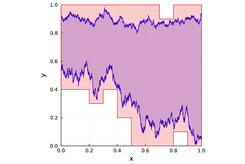
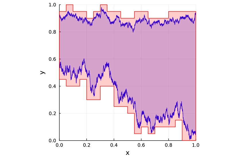
Figure 1.2: $\Lambda_{+}^{0}$ (blue) is approximated by the pixelated version $\Lambda_{+}^{\updownarrow}$ (red); left: $\delta=0.1$; right: $\delta=0.05$.

Based on a generalized Girsanov theorem for Itô processes, we can assign a modified local log-likelihood $\ell_{\delta,\alpha}(\vartheta_{-},\vartheta_{+},\Lambda_{+})$ to each $\alpha$-pixel for all pixelated candidate sets $\Lambda_{+}\in\mathcal{A}_{+}$ that assigns the diffusivity value $\vartheta_{\pm}$ to the $\alpha$-pixel if and only if $x_{\alpha}\in\Lambda_{\pm}$. An estimator $(\widehat{\vartheta}_{-},\widehat{\vartheta}_{+},\widehat{\Lambda}_{+})$ is then obtained as the maximizer of the aggregated contrast function

$$(\vartheta_{-},\vartheta_{+},\Lambda_{+})\mapsto\sum_{\alpha}\ell_{\delta,\alpha}(\vartheta_{-},\vartheta_{+},\Lambda_{+}),$$

which may be referred to as a CUSUM approach in analogy to change point estimation problems. Let us emphasize that we only require $\Lambda^{\updownarrow}_{+}\in\mathcal{A}_{+}$ of the pixelated candidate sets $\mathcal{A}_{+}$, which, given specific information on the shape of the true domain $\Lambda^{0}_{+}$, allows for much more parsimonious choices than the canonical choice of all possible black and white $\delta^{-1}\times\delta^{-1}$-images. On a more technical note, to establish the convergence bound, we reformulate our estimator as an M-estimator based on an appropriate empirical process $\chi\mapsto Z_{\delta}(\chi)$, so that quite naturally, concentration analysis of $Z_{\delta}$ becomes key. The basic idea of taking $\widehat{\Lambda}_{+}$ as union of best explanatory pixels by optimizing over a given family of candidate sets originates from classical statistical image reconstruction methods [36, 20, 26, 25].

The convergence rate of our estimator $\widehat{\Lambda}_{+}$ is entirely characterized by the complexity of the separating hypersurface $\Gamma$ that induces a bias between the true domain $\Lambda^{0}_{+}$ and its pixelated version $\Lambda^{0}_{+}$. In particular, assuming that the set $\mathcal{B}$, describing the number of pixels that are sliced by $\Gamma$ into two parts of non-zero volume, is of size

$$\lvert\mathcal{B}\rvert\lesssim\delta^{-d+\beta},\quad\beta\in(0,1],$$ (1.4)

we show in Theorem 3.7 that

$$\operatorname{{\mathbb{E}}}[\bm{\lambda}(\widehat{\Lambda}_{+}\vartriangle\Lambda_{+}^{0})]\lesssim\delta^{\beta},$$

with the symmetric set difference $\vartriangle$. This result immediately entails estimation rates for $\Lambda^{0}_{+}$ in terms of the Minkowski dimension of its boundary. Furthermore, the estimation procedure results in the diffusivity parameter estimation rates $|\widehat{\vartheta}_{\pm}-\vartheta_{\pm}|=O_{\operatorname{{\mathbb{P}}}}(\delta^{\beta/2})$, which yields the same estimation rate for the diffusivity or “image” estimator $\widehat{\vartheta}\coloneq\widehat{\vartheta}_{+}\bm{1}_{\widehat{\Lambda}_{+}}+\widehat{\vartheta}_{-}\bm{1}_{\widehat{\Lambda}_{-}}$.

To make this general estimation strategy and result concrete, we apply it to two specific shape constraints on $\Lambda_{+}^{0}$. Assuming that $\Gamma$ is a boundary fragment that is described by a change interface with graph representation $\tau^{0}\colon[0,1]^{d-1}\rightarrow[0,1]$, that is, $\Lambda_{+}^{0}=\{(x,y)\in[0,1]^{d}:y>\tau^{0}(x)\}$, we choose closed epigraphs of piecewise constant grid functions $\tau\colon[0,1]^{d-1}\to[0,1]$ as candidate sets $\mathcal{A}_{+}$. The boundary of the estimator $\widehat{\Lambda}_{+}$ may then be interpreted as the epigraph of a random function $\widehat{\tau}\colon[0,1]^{d-1}\to[0,1]$ that gives a nonparametric estimator of the true change interface $\tau^{0}$. Then, given $\beta$-Hölder smoothness assumptions on $\tau^{0}$, where $\beta\in(0,1],$ we can verify (1.4) and obtain

$$\operatorname{{\mathbb{E}}}[\lVert\widehat{\tau}-\tau^{0}\rVert_{L^{1}([0,1]^{d-1})}]\lesssim\delta^{\beta}\quad\text{or equivalently}\quad\operatorname{{\mathbb{E}}}[\bm{\lambda}(\widehat{\Lambda}_{+}\vartriangle\Lambda_{+}^{0})]\lesssim\delta^{\beta}.$$

In a second model, we assume that $\Lambda_{+}^{0}$ is a convex set with boundary $\Gamma$. Based on the observation that any ray that intersects the interior of a convex set does so in exactly two points, we construct a family of candidate sets $\mathcal{A}_{+}$ of size $\lvert\mathcal{A}_{+}\rvert\asymp\delta^{-(d+1)}$ and show that

$$\operatorname{{\mathbb{E}}}[\bm{\lambda}(\widehat{\Lambda}_{+}\vartriangle\Lambda^{0}_{+})]\lesssim\delta.$$

Optimality of the obtained rates in both models is discussed in the related image reconstruction problem.

Outline

The paper is structured as follows. In Section 2 we formalize the model and discuss fundamental properties of the solution to (1.1). The general estimation strategy and our main result is given in Section 3. In Section 4, those findings are applied to the two explicitly studied change domain structures outlined above. Lastly, we summarize our results and discuss potential extensions in future work in Section 5.

Notation

Throughout this paper, we work on a filtered probability space $(\Omega,\mathcal{F},(\mathcal{F}_{t})_{0\leq t\leq T},\operatorname{{\mathbb{P}}})$ with fixed time horizon $T<\infty$. The resolution level $\delta$ is such that $n\coloneq\delta^{-1}\in\operatorname{{\mathbb{N}}}$ and $N\coloneq n^{d}.$ For a set $A\subset\operatorname{{\mathbb{R}}}^{d}$, the notation $A^{\circ}$ is exclusively reserved for its interior in $\operatorname{{\mathbb{R}}}^{d}$ endowed with the standard Euclidean topology. For a general topological space $\mathcal{X}$ and a subset $A\subset\mathcal{X}$, we denote its interior by $\operatorname{int}A$, let $\overline{A}$ be its closure and $\partial A$ be its boundary in $\mathcal{X}$. If not mentioned explicitly otherwise, we always understand the topological space in this paper to be $\mathcal{X}=[0,1]^{d}$ endowed with the standard subspace topology. For two numbers $a,b\in\operatorname{{\mathbb{R}}}$, we write $a\lesssim b$ if $a\leq Cb$ holds for a constant $C$ that does not depend on $\delta$. For an open set $U\subset\operatorname{{\mathbb{R}}}^{d}$, $L^{2}(U)$ is the usual $L^{2}$-space with inner product $\sc{\cdot}{\cdot}_{L^{2}(U)}$ and we set $\sc{\cdot}{\cdot}\coloneq\sc{\cdot}{\cdot}_{L^{2}(\Lambda)}$. The Euclidean norm of a vector $a\in\operatorname{{\mathbb{R}}}^{p}$ is denoted by $\lvert a\rvert$. If $f\colon\operatorname{{\mathbb{R}}}^{d}\to\operatorname{{\mathbb{R}}}^{d}$ is a vector valued function, we write $\lVert f\rVert_{L^{2}(\operatorname{{\mathbb{R}}}^{d})}\coloneq\lVert\lvert f\rvert\rVert_{L^{2}(\operatorname{{\mathbb{R}}}^{d})}$. By $H^{k}(U)$ we denote the usual Sobolev spaces, and let $H_{0}^{1}(U)$ be the completion of $C_{c}^{\infty}(U)$, the space of smooth compactly supported functions, relative to the $H^{1}(U)$ norm. The gradient, divergence and Laplace operator are denoted by $\nabla$, $\nabla\cdot$ and $\Delta$, respectively.

2 Setup

We start by formally introducing the SPDE model, discussing existence of solutions and introducing the local measurement observation scheme that we will be working with in our statistical analysis.

2.1 The SPDE model

In the following we consider a stochastic partial differential equation on $\Lambda\coloneq(0,1)^{d}$, where $d\geq 2$, with Dirichlet boundary condition, which is specified by

$$\begin{cases}\mathop{}\!\mathrm{d}X(t)=\Delta_{\vartheta}X(t)\mathop{}\!\mathrm{d}t+\mathop{}\!\mathrm{d}W(t),&0\leq t\leq T,\\ X(0)\equiv 0,\\ X(t)|_{\partial_{\Lambda}}=0,&0\leq t\leq T,\end{cases}$$ (2.1)

for driving space-time white noise $(\dot{W}(t))_{t\in[0,T]}$ on $L^{2}(\Lambda)$. The operator $\Delta_{\vartheta}$ with domain $\mathcal{D}(\Delta_{\vartheta})$ is given formally by

$$\Delta_{\vartheta}u=\nabla\cdot\vartheta\nabla u=\sum_{i=1}^{d}\partial_{i}(\vartheta\partial_{i}u),\quad u\in\mathcal{D}(\Delta_{\vartheta}),$$ (2.2)

where $\vartheta$ is piecewise constant in space, given by

$$\vartheta(x)=\vartheta_{-}\mathbf{1}_{\Lambda_{-}}(x)+\vartheta_{+}\mathbf{1}_{\Lambda_{+}}(x),\quad x\in(0,1)^{d},$$

for two measurable and disjoint sets $\Lambda_{\pm}$ s.t. $\Lambda_{-}\cup\Lambda_{+}=[0,1]^{d}$ and $\vartheta_{-},\vartheta_{+}\in[\underline{\vartheta},\overline{\vartheta}]\subset(0,\infty)$. Equivalently, we may rewrite the diffusivity in terms of the jump height $\eta\coloneq\vartheta_{+}-\vartheta_{-}$ as

$$\vartheta(x)=\vartheta_{-}+\eta\bm{1}_{\Lambda_{+}}(x),\quad x\in(0,1)^{d}.$$

Under these assumptions, $\Delta_{\vartheta}$ is a uniformly elliptic divergence-form operator. We assume that $\Lambda_{-}$ and $\Lambda_{+}$ are separated by a hypersurface $\Gamma$ parameterizing the set of points in the intersection of the boundaries

$$\Gamma\coloneq\partial\Lambda_{+}=\partial\Lambda_{-}\subset[0,1]^{d},$$ (2.3)

where $\partial\Lambda_{\pm}$ denotes the boundary of $\Lambda_{\pm}$ as a subset of the topological space $[0,1]^{d}$. We are mainly interested in estimating the domain $\Lambda_{+}$ which is intrinsically related to $\Gamma.$ We first propose a general estimator based on local measurements of the solution on a uniform grid of hypercubes, whose convergence properties are determined by the complexity of the boundary $\Gamma$ measured in terms of the number of hypercubes that are required to cover it.

The more structural information we are given on the set $\Lambda_{+}$, the better we can fine-tune the family of candidate sets underlying the estimator in order to increase the feasibility of implementation. Specifically, we will consider two different models for $\Lambda_{\pm}$.

Model A: Graph representation

$\Gamma$ forms a boundary fragment that has a graph representation, denoted by a change interface $\tau\colon[0,1]^{d-1}\rightarrow[0,1],$ i.e.,

$$\Gamma=\big{\{}(x,\tau(x)):x\in[0,1]^{d-1}\big{\}}$$ (2.4)

and the set $\Lambda_{+}$ takes the form

$$\Lambda_{+}=\{(x,y)\in[0,1]^{d}:y>\tau(x)\}.$$

Accordingly, the estimation problem of identifying $\Lambda_{\pm}$ can equivalently be broken down to the nonparametric estimation of the function $\tau$. Specifically, for an estimator $\widehat{\tau}$ of $\tau$ we let $\widehat{\Lambda}_{+}\coloneq\overline{\{(x,y)\in[0,1]^{d}:y>\widehat{\tau}(x)\}}$ be the closure of the epigraph of $\widehat{\tau}$ and $\widehat{\Lambda}_{-}\coloneq[0,1]^{d}\setminus\widehat{\Lambda}_{+}$ be its complement. This gives

$$\operatorname{{\mathbb{E}}}\big{[}\bm{\lambda}\big{(}\widehat{\Lambda}_{\pm}\vartriangle\Lambda_{\pm}\big{)}\big{]}=\operatorname{{\mathbb{E}}}\big{[}\lVert\widehat{\tau}-\tau\rVert_{L^{1}([0,1]^{d-1})}\big{]},$$ (2.5)

such that evaluating the quality of the domain estimators $\widehat{\Lambda}_{\pm}$ measured in terms of the expected Lebesgue measure of the symmetric differences $\widehat{\Lambda}_{\pm}\vartriangle\Lambda_{\pm}$, is equivalent to studying the $L^{1}$-risk of the nonparametric estimator $\widehat{\tau}$ of the change interface.

Model B: Convex set

$\Lambda_{+}$ is convex. By convexity, for any $x\in\operatorname{int}\Lambda_{+}^{0}$, the vertical ray $y\mapsto x+ye_{d}$ intersects $\partial\Lambda_{+}$ in exactly two points and those intersection points can be modeled by a lower convex function $f_{1}$ and an upper concave function $f_{2}$. Estimation of $\Lambda_{+}$ is then heuristically speaking equivalent to the estimation of the upper and lower function, taking the closure of $\{(x,y)\in[0,1]^{d}:\widehat{f}_{1}(x)\leq y\leq\widehat{f}_{2}(x)\}$ as an estimator for $\Lambda_{+}.$

2.2 Characterization of the solution

We shall first discuss properties of the operator $\Delta_{\vartheta}$ based on general theory of elliptic divergence form operators with measurable coefficients from [12]. Let the closed quadratic form $\mathcal{E}_{\vartheta}$ with domain $\mathcal{D}(\mathcal{E}_{\vartheta})$ be given by

$$\begin{cases}\mathcal{D}(\mathcal{E_{\vartheta}})=H^{1}_{0}(\Lambda),\\ \mathcal{E}_{\vartheta}(u,v)=\int_{\Lambda}\vartheta\nabla u\cdot\nabla v.\end{cases}$$

By [12, Theorem 1.2.1], $\mathcal{E}_{\vartheta}$ is the form of a positive self-adjoint operator $-\Delta_{\vartheta}$ on $L^{2}(\Lambda)$ in the sense that $\lVert(-\Delta_{\vartheta})^{1/2}u\rVert^{2}=\mathcal{E}_{\vartheta}(u,u)$ for $\mathcal{D}((-\Delta_{\vartheta})^{1/2})=\mathcal{D}(\mathcal{E}_{\vartheta})$ and according to [12, Theorem 1.2.7], we have $u\in\mathcal{D}(-\Delta_{\vartheta})\subset H^{1}_{0}(\Lambda)$ if there exists $g\in L^{2}(\Lambda)$ such that for any $v\in C_{c}^{\infty}(\Lambda)$,

$$\mathcal{E}_{\vartheta}(u,v)=\int_{\Lambda}gv,$$

in which case $-\Delta_{\vartheta}u=g$. Thus, (2.2) can be interpreted in a distributional sense and we have the relation

$$\mathcal{E}_{\vartheta}(u,v)=-\sc{\Delta_{\vartheta}u}{v},\quad(u,v)\in\mathcal{D}(\Delta_{\vartheta})\times\mathcal{D}(\mathcal{E}_{\vartheta}).$$

Moreover, [12, Theorem 1.3.5] shows that $\mathcal{E}_{\vartheta}$ is a Dirichlet form, whence $\Delta_{\vartheta}$ generates a strongly continuous, symmetric semigroup $(S_{\vartheta}(t))_{t\geq 0}\coloneq(\exp(\Delta_{\vartheta}t))_{t\geq 0}$. The spectrum of $\Delta_{\vartheta}$ is discrete and the minimal eigenvalue, denoted by $\underline{\lambda}$, is strictly positive, cf. [13, Theorem 6.3.1]. Thus, $(-\Delta_{\vartheta})^{-1}$ exists as a bounded linear operator with domain $L^{2}(\Lambda)$ and we may fix an orthonormal basis $\{e_{k},k\in\operatorname{{\mathbb{N}}}\}$ consisting of eigenvectors corresponding to the eigenvalues $\{\lambda_{k},k\in\operatorname{{\mathbb{N}}}\}=\sigma(-\Delta_{\vartheta})$ that we denote in increasing order. Using the heat kernel bounds for the transition density of $S_{\vartheta}(t)$ given in [12, Corollary 3.2.8], it follows that for any $t>0$, $S_{\vartheta}(t)$ is a Hilbert–Schmidt operator, but no weak or mild solution to (2.1) in the sense of [11, Theorem 5.4] exists in $L^{2}((0,1)^{d})$ since $d\geq 2$ implies that $\int_{0}^{T}\lVert S_{\vartheta}(t)\rVert^{2}_{\mathrm{HS}}\mathop{}\!\mathrm{d}t=\infty$.

However, following the discussion in [4, Section 2.1] and [5, Section 6.4], taking into account that by [13, Theorem 6.3.1] we have $\lambda_{k}\asymp k^{2/d}$ for any $k\in\operatorname{{\mathbb{N}}}$, the stochastic convolution

$$X(t)\coloneq\int_{0}^{t}S_{\vartheta}(t-s)\mathop{}\!\mathrm{d}{W(s)},\quad t\in[0,T],$$

is well-defined as a stochastic process on the embedding space $\mathcal{H}_{1}\supset L^{2}((0,1)^{d})$, where $\mathcal{H}_{1}$ can be chosen as a Sobolev space of negative order $-s<-d/2+1$ that is induced by the eigenbasis $(\lambda_{k},e_{k})_{k\in\operatorname{{\mathbb{N}}}}$. Extending the dual pairings $\langle X(t),z\rangle_{\mathcal{H}_{1}\times\mathcal{H}^{\prime}_{1}}$ then allows us to obtain a Gaussian process $(\langle X(t),z\rangle)_{t\in[0,T],z\in L^{2}((0,1)^{d})}$ given by

$$\sc{X(t)}{z}\coloneq\int_{0}^{t}\sc{S_{\vartheta}(t-s)z}{\mathop{}\!\mathrm{d}W(s)},\quad t\in[0,T],\quad z\in L^{2}((0,1)^{d}),$$

that solves the SPDE in the sense that for any $z\in\mathcal{D}(\Delta_{\vartheta})$,

$$\sc{X(t)}{z}=\int_{0}^{t}\sc{X(s)}{\Delta_{\vartheta}z}\mathop{}\!\mathrm{d}s+\sc{W(t)}{z},\quad t\in[0,T],\quad z\in L^{2}((0,1)^{d}).$$ (2.6)

2.3 Local measurements

We decompose $[0,1]^{d}$ into $n^{d}$ closed $d$-dimensional hypercubes $(\operatorname{Sq}(\alpha))_{\alpha\in[n]^{d-1}}$, where $\operatorname{Sq}(\alpha)$ has edge length $\delta$ and is centered at $x_{\alpha}\coloneq\delta(\alpha-\tfrac{1}{2}\bm{1})$ for any $\alpha\in[n]^{d}$. By $\operatorname{Sq}(\alpha)^{\circ}$ we denote the interior of $\operatorname{Sq}(\alpha)$ in $\operatorname{{\mathbb{R}}}^{d}$. Let also $\mathfrak{P}\coloneq 2^{\{\operatorname{Sq}(\alpha):\alpha\in[n]^{d}\}}$ be the power set of $\{\operatorname{Sq}(\alpha):\alpha\in[n]^{d}\}$ and let $\mathcal{P}\coloneq\{\bigcup_{C\in\mathfrak{C}}C:\mathfrak{C}\in\mathfrak{P}\}$ be the family of sets that can be built from taking unions of hypercubes in $\{\operatorname{Sq}(\alpha):\alpha\in[n]^{d}\}$. We refer to the hypercubes $\operatorname{Sq}(\alpha)$ as tiles and for any set $A\subset[0,1]^{d}$ we call a set $C\in\mathcal{P}$ such that $A\subset C$ a tiling of $A$.

Our estimation procedure is based on continuous-time observations of

$$X_{\delta,\alpha}(t)=\langle X(t),K_{\delta,\alpha}\rangle,\quad X^{\Delta}_{\delta,\alpha}(t)=\langle X(t),\Delta K_{\delta,\alpha}\rangle,\quad\alpha\in[n]^{d},\quad 0\leq t\leq T,$$

with $K_{\delta,\alpha}(y)=\delta^{-d/2}K(\delta(y-x_{\alpha}))$, and $K\colon\operatorname{{\mathbb{R}}}^{d}\to\operatorname{{\mathbb{R}}}$ a kernel function such that $\operatorname{supp}K\subset[-1/2,1/2]^{d}$ and $K\in H^{2}(\operatorname{{\mathbb{R}}}^{d})$. The measurement points $x_{\alpha}$, $\alpha\in[n]^{d},$ are separated by an Euclidean distance of order $\delta$ such that the supports of the $K_{\delta,\alpha}$ are non-overlapping. In other words, we have $N=\delta^{-d}$ measurement locations. Note that $K_{\delta,\alpha}\in\mathcal{D}(\Delta_{\vartheta})$ whenever $\operatorname{supp}K_{\delta,\alpha}\cap\partial\Lambda_{+}=\varnothing,$ since then $\vartheta$ is constant on the support of $K_{\delta,\alpha}$. Thus, for $g=-\vartheta(x_{\alpha})\Delta K_{\delta,\alpha}$, integration by parts reveals $\int_{\Lambda}gv=\int_{\Lambda}\vartheta\nabla K_{\delta,\alpha}\cdot\nabla v$ for any $v\in C_{c}^{\infty}(\Lambda)$, i.e., $g=-\Delta_{\vartheta}K_{\delta,\alpha}$.

3 Estimation strategy and main result

From here on, we denote the truth, i.e., the true values of the diffusivity and the true set partition of $\Lambda$, by an additional superscript $0$ for statistical purposes. To avoid some technicalities, we impose from now on the following assumption on $\Lambda^{0}_{+}$.

Assumption 3.1.

$\Lambda^{0}_{+}$ is open in $[0,1]^{d}$.

Since we are primarily interested in recovering the change domain $\Lambda_{+}^{0}$ and therefore treat the diffusivity parameters $\vartheta^{0}_{\pm}$ as nuisance parameters, we also make the following, slightly restricting assumption throughout the remainder of the paper:

Assumption 3.2.

We have access to two compact sets $\Theta_{-},\Theta_{+}\subset[\underline{\vartheta},\overline{\vartheta}]$ such that

1. $\vartheta^{0}_{-}\in\Theta_{-}$ and $\vartheta^{0}_{+}\in\Theta_{+},$ and

2. $\Theta_{-}$ and $\Theta_{+}$ are separated by $\underline{\eta}>0$, i.e., for any $\vartheta_{-}\in\Theta_{-}$ and $\vartheta_{+}\in\Theta_{+}$, it holds $\lvert\vartheta_{+}-\vartheta_{-}\rvert\geq\underline{\eta}.$

In particular, this assumption implies that we have access to a lower bound $\underline{\eta}>0$ on the absolute diffusivity jump height $\lvert\eta^{0}\rvert=\lvert\vartheta^{0}_{+}-\vartheta^{0}_{-}\rvert$. For some set $C\subset[0,1]^{d}$ define

$$C^{+}\coloneq\bigcup_{\alpha\in[n]^{d}:\operatorname{Sq}(\alpha)^{\circ}\cap C\neq\varnothing}\operatorname{Sq}(\alpha),$$

which, if $C$ is open in $[0,1]^{d}$, is the minimal tiling of $C$, so that in particular $C\subset C^{+}\in\mathcal{P}$. Let us also set

$$\Lambda^{\updownarrow}_{+}\coloneq(\Lambda^{0}_{+})^{+},$$

which is the minimal tiling of $\Lambda^{0}_{+}$ by our assumption that $\Lambda^{0}_{+}$ is open in $[0,1]^{d}$. Let $\mathcal{A}_{+}\subset\mathcal{P}$ be a family of candidate sets for a tiling of $\Lambda^{0}_{+}$ such that $\Lambda^{\updownarrow}_{+}\in\mathcal{A_{+}}$. Note that $\mathcal{A}_{+}=\mathcal{P}$ is always a valid choice. However, as we shall see later, much more parsimonious choices are possible if we can assume some structure on the set $\Lambda_{+}^{0}.$ We now introduce the modified local log-likelihood

$$\ell_{\delta,\alpha}(\vartheta_{-},\vartheta_{+},\Lambda_{+})=\vartheta_{\delta,\alpha}(\Lambda_{+})\int_{0}^{T}X^{\Delta}_{\delta,\alpha}(t)\mathop{}\!\mathrm{d}{X_{\delta,\alpha}(t)}-\frac{\vartheta_{\delta,\alpha}(\Lambda_{+})^{2}}{2}\int_{0}^{T}X^{\Delta}_{\delta,\alpha}(t)^{2}\mathop{}\!\mathrm{d}{t},$$ (3.1)

for the decision rule

$$\vartheta_{\delta,\alpha}(\Lambda_{+})\coloneq\begin{cases}\vartheta_{+},&\operatorname{Sq}(\alpha)\subset\Lambda_{+},\\ \vartheta_{-},&\text{else},\end{cases}=\begin{cases}\vartheta_{+},&x_{\alpha}\in\Lambda_{+},\\ \vartheta_{-},&\text{else},\end{cases}$$ (3.2)

where $\vartheta_{\pm}\in\Theta_{\pm}$ and the candidate sets $\Lambda_{+}\in\mathcal{A}_{+}$ are anchored on the grid $\mathcal{P}$ spanned by the hypercubes $\operatorname{Sq}(\alpha)$. The interpretation of the stochastic integral in (3.1) is provided by the following result that characterizes the tested processes $X_{\delta,\alpha}$ as semimartingales whose dynamics are determined by the location of the hypercube $\operatorname{Sq}(\alpha)$ relative to $\Lambda^{0}_{\pm}$.

Proposition 3.3 (Modification of Proposition 2.1 in [30]).

For any $\alpha\in[n]^{d}$ and $t\in[0,T]$ we have

$$X_{\delta,\alpha}(t)=\begin{cases}\vartheta_{-}^{0}\int_{0}^{t}X^{\Delta}_{\delta,\alpha}(s)\mathop{}\!\mathrm{d}s+B_{\delta,\alpha}(t),&\operatorname{Sq}(\alpha)\subset\overline{\Lambda_{-}^{0}},\\ \vartheta_{+}^{0}\int_{0}^{t}X^{\Delta}_{\delta,\alpha}(s)\mathop{}\!\mathrm{d}s+B_{\delta,\alpha}(t),&\operatorname{Sq}(\alpha)\subset\overline{\Lambda_{+}^{0}},\\ \int_{0}^{t}\int_{0}^{s}\sc{\Delta_{\vartheta^{0}}S_{\vartheta^{0}}(s-u)K_{\delta,\alpha}}{\mathop{}\!\mathrm{d}W(u)}\mathop{}\!\mathrm{d}s+B_{\delta,\alpha}(t),&\text{else},\end{cases}$$

where $(B_{\delta,\alpha})_{\alpha\in[n]^{d}}$ is an $n^{d}$-dimensional vector of independent scalar Brownian motions.

Proof.

The first two lines follow from (2.6) using $K_{\delta,\alpha}\in\mathcal{D}(\Delta_{\vartheta^{0}})$ if $\operatorname{supp}K_{\delta,\alpha}\cap\partial\Lambda_{-}\cap\partial\Lambda_{+}=\varnothing,$ in which cases $\Delta_{\vartheta^{0}}K_{\delta,\alpha}=\vartheta_{-}^{0}\Delta K_{\delta,\alpha}$ and $\Delta_{\vartheta}K_{\delta,\alpha}=\vartheta_{+}^{0}\Delta K_{\delta,\alpha}$, respectively. The expression on the change areas, where generally $K_{\delta,\alpha}\notin\mathcal{D}(\Delta_{\vartheta^{0}})$, is proven in complete analogy to [30, Lemma A.1] using spectral calculus and the stochastic Fubini theorem. ∎

We employ a CUSUM estimation approach based on the local log-likelihoods in (3.1) and therefore specify an estimator $(\widehat{\vartheta}_{-},\widehat{\vartheta}_{+},\widehat{\Lambda}_{+})$ via

$$(\widehat{\vartheta}_{-},\widehat{\vartheta}_{+},\widehat{\Lambda}_{+})\in\operatorname*{arg\,max}_{(\vartheta_{-},\vartheta_{+},\Lambda_{+})\in\Theta_{-}\times\Theta_{+}\times\mathcal{A}_{+}}\sum_{\alpha\in[n]^{d}}\ell_{\delta,\alpha}(\vartheta_{-},\vartheta_{+},\Lambda_{+}).$$ (3.3)

Here, the set of maximizers is well defined and we can make a measurable choice for a maximizer since $\Theta_{\pm}$ are compact and $\mathcal{A}_{+}$ is a finite set. Setting

$$\widehat{\Lambda}_{-}\coloneq[0,1]^{d}\setminus\widehat{\Lambda}_{+},$$

as the corresponding estimator of $\Lambda^{0}_{-}$ we obtain the nonparametric diffusivity estimator

$$\widehat{\vartheta}(x)\coloneq\widehat{\vartheta}_{-}\bm{1}_{\widehat{\Lambda}_{-}}(x)+\widehat{\vartheta}_{+}\bm{1}_{\widehat{\Lambda}_{+}}(x),\quad x\in(0,1)^{d-1}.$$

Introduce further

$$\vartheta^{0}_{\delta,\alpha}\coloneq\begin{cases}\vartheta^{0}_{+},&\operatorname{Sq}(\alpha)\subset\Lambda_{+}^{\updownarrow},\\ \vartheta^{0}_{-},&\text{else},\end{cases}=\begin{cases}\vartheta^{0}_{+},&x_{\alpha}\in\Lambda^{\updownarrow}_{+}\\ \vartheta^{0}_{-},&\text{else},\end{cases}$$ (3.4)

and define by

$$\begin{split}\mathcal{B}&=\{\alpha\in[n]^{d}:\operatorname{Sq}(\alpha)^{\circ}\cap\partial\Lambda_{+}^{0}\neq\emptyset\},\end{split}$$

the indices $\alpha$ of hypercubes whose interiors intersect the boundary of $\Lambda^{0}_{+}$. It is important to observe that the boundary tiles $\mathcal{B}$ may equivalently be expressed as follows.

Lemma 3.4.

It holds that

$$\mathcal{B}=\{\alpha\in[n]^{d}:\operatorname{Sq}(\alpha)^{\circ}\cap(\Lambda^{\updownarrow}_{+}\vartriangle\Lambda^{0}_{+})\neq\varnothing\}.$$

Proof.

Since $\Lambda^{0}_{+}$ is open in $[0,1]^{d}$, it holds that $\Lambda^{0}_{+}\subset\Lambda^{\updownarrow}_{+}$ and therefore $\Lambda^{\updownarrow}_{+}\vartriangle\Lambda^{0}_{+}=\Lambda^{\updownarrow}_{+}\setminus\Lambda^{0}_{+}$. Since $\Lambda^{\updownarrow}_{+}$ is closed and $\partial\Lambda^{0}_{+}\cap\Lambda^{0}_{+}=\varnothing$, it follows that $\partial\Lambda^{0}_{+}\subset\Lambda^{\updownarrow}_{+}\vartriangle\Lambda^{0}_{+}$, which gives the inclusion

$$\mathcal{B}\subset\{\alpha\in[n]^{d}:\operatorname{Sq}(\alpha)^{\circ}\cap(\Lambda^{\updownarrow}_{+}\vartriangle\Lambda^{0}_{+})\neq\varnothing\}.$$

Conversely, if $\varnothing\neq\operatorname{Sq}(\alpha)^{\circ}\cap(\Lambda^{\updownarrow}_{+}\vartriangle\Lambda^{0}_{+})=\operatorname{Sq}(\alpha)^{\circ}\cap(\Lambda^{\updownarrow}_{+}\setminus\Lambda^{0}_{+})$, it follows that $\operatorname{Sq}(\alpha)^{\circ}\not\subset\Lambda^{0}_{+}$, but $\operatorname{Sq}(\alpha)\subset\Lambda^{\updownarrow}_{+}$ since the latter belongs to $\mathcal{P}.$ Thus, by definition of $\Lambda^{\updownarrow}_{+}$, we have $\operatorname{Sq}(\alpha)^{\circ}\cap\Lambda^{0}_{+}\neq\varnothing$, which because $\operatorname{Sq}(\alpha)^{\circ}$ is connected and $\operatorname{Sq}(\alpha)^{\circ}\not\subset\Lambda^{0}_{+}$ implies that $\operatorname{Sq}(\alpha)^{\circ}\cap\partial\Lambda^{0}_{+}\neq\varnothing$. This now also yields

$$\mathcal{B}\supset\{\alpha\in[n]^{d}:\operatorname{Sq}(\alpha)^{\circ}\cap(\Lambda^{\updownarrow}_{+}\vartriangle\Lambda^{0}_{+})\neq\varnothing\}.$$

∎

Plugging the given representation of Proposition 3.3 into (3.1), we may now express $\ell_{\delta,\alpha}$ in the following way,

$$\ell_{\delta,\alpha}(\vartheta_{-},\vartheta_{+},\Lambda_{+}) =\big{(}\vartheta_{\delta,\alpha}(\Lambda_{+})\vartheta^{0}_{\delta,\alpha}-\vartheta_{\delta,\alpha}(\Lambda_{+})^{2}/2\big{)}I_{\delta,\alpha}+\vartheta_{\delta,\alpha}(\Lambda_{+})M_{\delta,\alpha}$$

$$\quad+\bm{1}_{\mathcal{B}}(\alpha)\vartheta_{\delta,\alpha}(\Lambda_{+})R_{\delta,\alpha},$$

where we denote

$$M_{\delta,\alpha}\coloneq\int_{0}^{T}X^{\Delta}_{\delta,\alpha}(t)\mathop{}\!\mathrm{d}{B_{\delta,\alpha}(t)},\quad I_{\delta,\alpha}\coloneq\int_{0}^{T}X^{\Delta}_{\delta,\alpha}(t)^{2}\mathop{}\!\mathrm{d}{t},$$

and

$$R_{\delta,\alpha}\coloneq\int_{0}^{T}X^{\Delta}_{\delta,\alpha}(t)\Big{(}\int_{0}^{t}\langle\Delta_{\vartheta^{0}}S_{\vartheta^{0}}(t-s)K_{\delta,\alpha}-\vartheta^{0}_{+}S_{\vartheta^{0}}(t-s)\Delta K_{\delta,\alpha},\mathop{}\!\mathrm{d}{W}(s)\rangle\Big{)}\mathop{}\!\mathrm{d}{t}.$$

The estimator (3.3) therefore can be represented as

$$(\widehat{\vartheta}_{-},\widehat{\vartheta}_{+},\widehat{\Lambda}_{+}) \in\operatorname*{arg\,max}_{(\vartheta_{-},\vartheta_{+},\Lambda_{+})\in\Theta_{-}\times\Theta_{+}\times\mathcal{A}_{+}}\Big{\{}\sum_{\alpha\in[n]^{d}}\Big{(}(\vartheta_{\delta,\alpha}(\Lambda_{+})-\vartheta^{0}_{\delta,\alpha})M_{\delta,\alpha}-\frac{1}{2}(\vartheta_{\delta,\alpha}(\Lambda_{+})-\vartheta^{0}_{\delta,\alpha})^{2}I_{\delta,\alpha}\Big{)}$$

$$\hskip 60.0pt+\sum_{\alpha\in\mathcal{B}}\vartheta_{\delta,\alpha}(\Lambda_{+})R_{\delta,\alpha}+\sum_{\alpha\in[n]^{d}}\Big{(}\vartheta^{0}_{\delta,\alpha}M_{\delta,\alpha}+\frac{(\vartheta^{0}_{\delta,\alpha})^{2}}{2}I_{\delta,\alpha}\Big{)}\Big{\}}$$

$$=\operatorname*{arg\,min}_{(\vartheta_{-},\vartheta_{+},\Lambda_{+})\in\Theta_{-}\times\Theta_{+}\times\mathcal{A}_{+}}\Big{\{}Z_{\delta}(\vartheta_{-},\vartheta_{+},\Lambda_{+})-\sum_{\alpha,\in\mathcal{B}}\vartheta_{\delta,\alpha}(\Lambda_{+})R_{\delta,\alpha}\Big{\}},$$ (3.5)

where the empirical process $Z_{\delta}(\cdot)$ is given by

$$\begin{split}Z_{\delta}(\vartheta_{-},\vartheta_{+},\Lambda_{+})&\coloneq\sum_{\alpha\in[n]^{d}}\frac{1}{2}(\vartheta_{\delta,\alpha}(\Lambda_{+})-\vartheta^{0}_{\delta,\alpha})^{2}I_{\delta,\alpha}-\sum_{\alpha\in[n]^{d}}(\vartheta_{\delta,\alpha}(\Lambda_{+})-\vartheta^{0}_{\delta,\alpha})M_{\delta,\alpha}\\ &=\frac{1}{2}I_{T,\delta}(\vartheta_{-},\vartheta_{+},\Lambda_{+})-M_{T,\delta}(\vartheta_{-},\vartheta_{+},\Lambda_{+}),\end{split}$$ (3.6)

where

$$I_{T,\delta}(\vartheta_{-},\vartheta_{+},\Lambda_{+}) \coloneq\sum_{\alpha\in[n]^{d}}(\vartheta_{\delta,\alpha}(\Lambda_{+})-\vartheta^{0}_{\delta,\alpha})^{2}I_{\delta,\alpha},$$

$$M_{T,\delta}(\vartheta_{-},\vartheta_{+},\Lambda_{+}) \coloneq\sum_{\alpha\in[n]^{d}}(\vartheta_{\delta,\alpha}(\Lambda_{+})-\vartheta^{0}_{\delta,\alpha})M_{\delta,\alpha}.$$

Note in particular that $Z_{\delta}(\vartheta_{-}^{0},\vartheta_{+}^{0},\Lambda^{\updownarrow}_{+})=0$, so that $Z_{\delta}(\cdot)$ is centered around the truth $(\vartheta_{-}^{0},\vartheta^{0}_{+},\Lambda^{\updownarrow}_{+})$. It will be crucial to have good control on the empirical process $Z_{\delta}$, which is provided by the following lemma that specifies the order of the observed Fisher informations $I_{\delta,\alpha}$. The proof is a straightforward extension of the corresponding one-dimensional result [30, Lemma 3.3] using the analogous spectral arguments in higher dimensions and can therefore be omitted.

Lemma 3.5 (Modification of Lemma 3.3 in [30]).

• For any $\alpha\in[n]^{d}$ with $\alpha\notin\mathcal{B},$ it holds

  $$\operatorname{{\mathbb{E}}}[I_{\delta,\alpha}]=\frac{T}{2\vartheta_{\delta,\alpha}^{0}}\lVert\nabla K\rVert^{2}_{L^{2}(\operatorname{{\mathbb{R}}}^{d})}\delta^{-2}+O(1).$$

• For any $\alpha\in\mathcal{B},$ it holds

  $$\operatorname{{\mathbb{E}}}[I_{\delta,\alpha}]\in\left[\frac{2\underline{\lambda}T-1+\mathrm{e}^{-2\underline{\lambda}T}}{4\underline{\lambda}\overline{\vartheta}}\lVert\nabla K\rVert^{2}_{L^{2}(\operatorname{{\mathbb{R}}}^{d})}\delta^{-2},\frac{T}{2\underline{\vartheta}}\lVert\nabla K\rVert^{2}_{L^{2}(\operatorname{{\mathbb{R}}}^{d})}\delta^{-2}\right].$$

• For any vector $\beta\in(\operatorname{{\mathbb{R}}}^{n})^{d}$ with $\beta_{\alpha}=0$ if $\alpha\in\mathcal{B}$, we have

  $$\operatorname{Var}\Big{(}\sum_{\alpha\in[n]^{d}}\beta_{\alpha}I_{\delta,\alpha}\Big{)}\leq\frac{T}{2\underline{\vartheta}^{3}}\delta^{-2}\lVert\beta\rVert^{2}_{l^{2}}\lVert\nabla K\rVert^{2}_{L^{2}(\operatorname{{\mathbb{R}}}^{d})}.$$

Furthermore, convergence of the estimator $(\widehat{\vartheta}_{-},\widehat{\vartheta}_{+},\widehat{\Lambda}_{+})$ requires insight on the order of the remainders $R_{\delta,\alpha}$ in the representation (3.5), given by the following lemma.

Lemma 3.6.

For any $\alpha\in\mathcal{B}$ we have

$$\operatorname{{\mathbb{E}}}\big{[}\lvert R_{\delta,\alpha}\rvert\big{]}\lesssim\delta^{-2}.$$

Proof.

By Lemma 3.5 we know that $\operatorname{{\mathbb{E}}}[I_{\delta,\alpha}]\lesssim\delta^{-2}$ for any $\alpha\in[n]^{d}$. Since

$$R_{\delta,\alpha}=\int_{0}^{T}X^{\Delta}_{\delta,\alpha}(t)\int_{0}^{t}\langle\Delta_{\vartheta^{0}}S_{\vartheta^{0}}(t-s)K_{\delta,\alpha},\mathop{}\!\mathrm{d}{W(s)}\rangle\mathop{}\!\mathrm{d}{t}-\vartheta_{+}^{0}I_{\delta,\alpha},$$

it is enough to show

$$\operatorname{{\mathbb{E}}}\Big{[}\Big{\lvert}\int_{0}^{T}X^{\Delta}_{\delta,\alpha}(t)\int_{0}^{t}\langle\Delta_{\vartheta^{0}}S_{\vartheta^{0}}(t-s)K_{\delta,\alpha},\mathop{}\!\mathrm{d}{W(s)}\rangle\mathop{}\!\mathrm{d}{t}\Big{\rvert}\Big{]}\lesssim\delta^{-2}.$$ (3.7)

We have

$$\operatorname{{\mathbb{E}}}\Big{[}\Big{\lvert}\int_{0}^{T}X^{\Delta}_{\delta,\alpha}(t)\int_{0}^{t}\langle\Delta_{\vartheta^{0}}S_{\vartheta^{0}}(t-s)K_{\delta,\alpha},\mathop{}\!\mathrm{d}{W(s)}\rangle\mathop{}\!\mathrm{d}{t}\Big{\rvert}\Big{]}$$

$$\quad\leq\operatorname{{\mathbb{E}}}\big{[}I_{\delta,\alpha}\big{]}^{1/2}\operatorname{{\mathbb{E}}}\Big{[}\int_{0}^{T}\Big{(}\int_{0}^{t}\langle\Delta_{\vartheta^{0}}S_{\vartheta^{0}}(t-s)K_{\delta,\alpha},\mathop{}\!\mathrm{d}{W(s)}\rangle\Big{)}^{2}\mathop{}\!\mathrm{d}{t}\Big{]}^{1/2}$$

$$\quad\lesssim\delta^{-1}\Big{(}\operatorname{{\mathbb{E}}}\Big{[}\int_{0}^{T}\Big{(}\int_{0}^{t}\langle\Delta_{\vartheta^{0}}S_{\vartheta^{0}}(t-s)K_{\delta,\alpha},\mathop{}\!\mathrm{d}{W(s)}\rangle\Big{)}^{2}\mathop{}\!\mathrm{d}{t}\Big{]}\Big{)}^{1/2}$$

$$\quad=\delta^{-1}\Big{(}\int_{0}^{T}\int_{0}^{t}\big{\lVert}\Delta_{\vartheta^{0}}S_{\vartheta^{0}}(t-s)K_{\delta,\alpha}\big{\rVert}^{2}\mathop{}\!\mathrm{d}{s}\mathop{}\!\mathrm{d}{t}\Big{)}^{1/2},$$

where we used the Cauchy–Schwarz inequality for the first two inequalities and Fubini’s theorem together with the Itô-isometry for the last line. Since

$$\int_{0}^{T}\int_{0}^{t}\big{\lVert}\Delta_{\vartheta^{0}}S_{\vartheta^{0}}(t-s)K_{\delta,\alpha}\big{\rVert}^{2}\mathop{}\!\mathrm{d}{s}\mathop{}\!\mathrm{d}{t} \leq T\int_{0}^{T}\big{\lVert}\Delta_{\vartheta^{0}}S_{\vartheta^{0}}(t)K_{\delta,\alpha}\big{\rVert}^{2}\mathop{}\!\mathrm{d}{t}$$

$$=T\sum_{k\in\operatorname{{\mathbb{N}}}}\int_{0}^{T}\lambda_{k}^{2}\mathrm{e}^{-2\lambda_{k}t}\mathop{}\!\mathrm{d}{t}\langle e_{k},K_{\delta,\alpha}\rangle^{2}$$

$$\leq\frac{T}{2}\sum_{k\in\operatorname{{\mathbb{N}}}}\lambda_{k}\langle e_{k},K_{\delta,\alpha}\rangle^{2}$$

$$=\frac{T}{2}\big{\lVert}(-\Delta_{\vartheta^{0}})^{1/2}K_{\delta,\alpha}\big{\rVert}^{2}$$

$$=\frac{T}{2}\int_{\Lambda}\vartheta^{0}(x)\lvert\nabla K_{\delta,\alpha}(x)\rvert^{2}\mathop{}\!\mathrm{d}{x}$$

$$\leq\frac{T\overline{\vartheta}}{2}\lVert\nabla K_{\delta,\alpha}\rVert^{2}_{L^{2}(\operatorname{{\mathbb{R}}}^{d})}$$

$$=\delta^{-2}\frac{T\overline{\vartheta}\lVert\nabla K\rVert^{2}_{L^{2}(\operatorname{{\mathbb{R}}}^{d})}}{2},$$

the bound (3.7) follows, proving the assertion. ∎

We are now ready to prove our main result.

Theorem 3.7.

Suppose that for some $\beta\in(0,1]$ and some constant $c>0$ it holds that

$$\lvert\mathcal{B}\rvert\leq c\delta^{-d+\beta}.$$ (3.8)

Then, for some absolute constant $C$ depending only on $c,d,\underline{\vartheta},\overline{\vartheta},T$ and $\underline{\eta}$ it holds that

$$\operatorname{{\mathbb{E}}}\big{[}\bm{\lambda}(\widehat{\Lambda}_{+}\vartriangle\Lambda^{0}_{+})\big{]}\leq{C}\delta^{\beta}.$$

Proof.

Let $\chi^{0}\coloneq(\vartheta^{0}_{-},\vartheta^{0}_{+},(\Lambda^{0}_{+})^{+})=(\vartheta_{-}^{0},\vartheta_{+}^{0},\Lambda^{\updownarrow}_{+})$ and set for $\chi=(\vartheta_{-},\vartheta_{+},\Lambda_{+})\in\Theta_{-}\times\Theta_{+}\times\mathcal{A}_{+},$

$$L_{\delta}(\chi)=\delta^{d+2}Z_{\delta}(\vartheta_{-},\vartheta_{+},\Lambda_{+}),\quad\widetilde{L}_{\delta}(\chi)=\operatorname{{\mathbb{E}}}[L_{\delta}(\chi)].$$

We first observe that (3.5) implies

$$L_{\delta}(\widehat{\vartheta}_{-},\widehat{\vartheta}_{+},\widehat{\Lambda}_{+})\leq\min_{\chi\in\Theta_{-}\times\Theta_{+}\times\mathcal{A}_{+}}L_{\delta}(\chi)+2\delta^{2+d}\overline{\vartheta}\sum_{\alpha\in\mathcal{B}}\lvert R_{\delta,\alpha}\rvert.$$ (3.9)

Furthermore, since $L_{\delta}(\chi^{0})=0$ and $\operatorname{{\mathbb{E}}}[M_{\delta,\alpha}]=0$, we obtain with Lemma 3.5 that for any $\chi=(\vartheta_{-},\vartheta_{+},\Lambda_{+})\in\Theta_{-}\times\Theta_{+}\times\mathcal{A}_{+}$,

$$\begin{split}\widetilde{L}_{\delta}(\chi)-\widetilde{L}_{\delta}(\chi^{0})&=\operatorname{{\mathbb{E}}}[L_{\delta}(\chi)]\asymp\delta^{d}\sum_{\alpha\in[n]^{d}}(\vartheta_{\delta,\alpha}(\Lambda_{+})-\vartheta^{0}_{\delta,\alpha})^{2}\\ &=\delta^{d}\sum_{\alpha\in[n]^{d}:\operatorname{Sq}(\alpha)^{\circ}\subset(\Lambda_{+}\cap\Lambda^{\updownarrow}_{+})}(\vartheta_{+}-\vartheta^{0}_{+})^{2}+\delta^{d}\sum_{\alpha\in[n]^{d}:\operatorname{Sq}(\alpha)^{\circ}\subset(\Lambda_{+}\cup\Lambda_{+}^{\updownarrow})^{\mathrm{c}}}(\vartheta_{-}-\vartheta^{0}_{-})^{2}\\ &\quad+\delta^{d}\sum_{\alpha\in[n]^{d}:\operatorname{Sq}(\alpha)^{\circ}\subset(\Lambda_{+}\vartriangle\Lambda^{\updownarrow}_{+})}(\vartheta_{\delta,\alpha}(\Lambda_{+})-\vartheta^{0}_{\delta,\alpha})^{2}\\ &\geq\underline{\eta}^{2}\delta^{d}\big{\lvert}\big{\{}\alpha\in[n]^{d}:\operatorname{Sq}(\alpha)^{\circ}\subset(\Lambda_{+}\vartriangle\Lambda^{\updownarrow}_{+})\big{\}}\big{\rvert}\\ &=\underline{\eta}^{2}\bm{\lambda}(\Lambda_{+}\vartriangle\Lambda^{\updownarrow}_{+}),\end{split}$$ (3.10)

where for the penultimate line we observe that for $\operatorname{Sq}(\alpha)^{\circ}\subset(\Lambda_{+}\vartriangle\Lambda^{\updownarrow}_{+})$ we have $\vartheta_{\delta,\alpha}(\Lambda_{+})=\vartheta_{\pm}$ iff $\vartheta^{0}_{\delta,\alpha}=\vartheta^{0}_{\mp}$, and conclude with $\vartheta_{\pm},\vartheta^{0}_{\pm}\in\Theta_{\pm}$ and the fact that $\Theta_{+}$ and $\Theta_{-}$ are $\underline{\eta}$-separated. Now, using the characterization from Lemma (3.4) and the assumption (3.8), it follows that

$$\bm{\lambda}(\Lambda^{0}_{+}\vartriangle\Lambda^{\updownarrow}_{+})\leq\delta^{d}\lvert\mathcal{B}\rvert\leq c\delta^{\beta}.$$ (3.11)

Combined with (3.10), triangle inequality for the symmetric difference pseudometric therefore yields

$$\bm{\lambda}(\Lambda_{+}\vartriangle\Lambda^{0}_{+})\lesssim\widetilde{L}_{\delta}(\chi)-\widetilde{L}_{\delta}(\chi^{0})+\delta^{\beta},\quad\chi=(\vartheta_{-},\vartheta_{+},\Lambda_{+})\in\Theta_{-}\times\Theta_{+}\times\mathcal{A}_{+},$$

whence the assertion follows once we have verified that

$$\operatorname{{\mathbb{E}}}[\widetilde{L}_{\delta}(\widehat{\chi})-\widetilde{L}_{\delta}(\chi^{0})]\lesssim\delta^{\beta},\quad\widehat{\chi}\coloneq(\widehat{\vartheta}_{-},\widehat{\vartheta}_{+},\widehat{\Lambda}_{+}),$$ (3.12)

where by definition $\widetilde{L}_{\delta}(\widehat{\chi})=\operatorname{{\mathbb{E}}}[L_{\delta}(\chi)]|_{\chi=\widehat{\chi}}$. Taking into account (3.8), (3.9) and Lemma 3.6, we arrive at

$$\begin{split}\operatorname{{\mathbb{E}}}[\widetilde{L}_{\delta}(\widehat{\chi})-\widetilde{L}_{\delta}(\chi^{0})]&\leq\operatorname{{\mathbb{E}}}\big{[}\widetilde{L}_{\delta}(\widehat{\chi})-\widetilde{L}_{\delta}(\chi^{0})+L_{\delta}(\chi^{0})-L_{\delta}(\widehat{\chi})\big{]}\\ &\quad+2\delta^{d+2}c\delta^{\beta-d}\max_{\alpha\in\mathcal{B}}\operatorname{{\mathbb{E}}}[\lvert R_{\delta,\alpha}\rvert]\\ &\lesssim\operatorname{{\mathbb{E}}}\Big{[}\sup_{\chi\in\Theta_{-}\times\Theta_{+}\times\mathcal{A}_{+}}\lvert L_{\delta}(\chi)-\widetilde{L}_{\delta}(\chi)\rvert\Big{]}+\delta^{\beta}.\end{split}$$ (3.13)

To prove (3.12) it therefore remains to show

$$\operatorname{{\mathbb{E}}}\Big{[}\sup_{\chi\in\Theta_{-}\times\Theta_{+}\times\mathcal{A}_{+}}\lvert L_{\delta}(\chi)-\widetilde{L}_{\delta}(\chi)\rvert\Big{]}\lesssim\delta^{\beta},$$

which, recalling the decomposition (3.6) and using $\operatorname{{\mathbb{E}}}[M_{T,\delta}(\chi)]=0$, boils down to show

$$\operatorname{{\mathbb{E}}}\Big{[}\sup_{\chi\in\Theta_{-}\times\Theta_{+}\times\mathcal{A}_{+}}\lvert I_{T,\delta}(\chi)-\operatorname{{\mathbb{E}}}[I_{T,\delta}(\chi)]\rvert\Big{]} \lesssim\delta^{\beta-d-2},$$ (3.14)

$$\operatorname{{\mathbb{E}}}\Big{[}\sup_{\chi\in\Theta_{-}\times\Theta_{+}\times\mathcal{A}_{+}}\lvert M_{T,\delta}(\chi)\rvert\Big{]} \lesssim\delta^{\beta-d-2}.$$ (3.15)

Clearly, by triangle inequality, we get the rough bounds

$$\sup_{\chi\in\Theta_{-}\times\Theta_{+}\times\mathcal{A}_{+}}\lvert I_{T,\delta}(\chi)-\operatorname{{\mathbb{E}}}[I_{T,\delta}(\chi)]\rvert \leq(\overline{\vartheta}-\underline{\vartheta})^{2}\sum_{\alpha\in[n]^{d}}\lvert I_{\delta,\alpha}-\operatorname{{\mathbb{E}}}[I_{\delta,\alpha}]\rvert,$$

$$\sup_{\chi\in\Theta_{-}\times\Theta_{+}\times\mathcal{A}_{+}}\lvert M_{T,\delta}(\chi)\rvert \leq\lvert\overline{\vartheta}-\underline{\vartheta}\rvert\sum_{\alpha\in[n]^{d}}\lvert M_{\delta,\alpha}\rvert.$$

Thus, applying once more the assumption (3.8) and the bounds from Lemma 3.5,

$$\operatorname{{\mathbb{E}}}\Big{[}\sup_{\chi\in\Theta_{-}\times\Theta_{+}\times\mathcal{A}_{+}}\lvert I_{T,\delta}(\chi)-\operatorname{{\mathbb{E}}}[I_{T,\delta}(\chi)]\rvert\Big{]}$$

$$\,\lesssim\delta^{\beta-d}\max_{\alpha\in\mathcal{B}}\operatorname{{\mathbb{E}}}[\lvert I_{\delta,\alpha}-\operatorname{{\mathbb{E}}}[I_{\delta,\alpha}]\rvert]+\delta^{-d}\max_{\alpha\in[n]^{d}\setminus\mathcal{B}}\operatorname{{\mathbb{E}}}[\lvert I_{\delta,\alpha}-\operatorname{{\mathbb{E}}}[I_{\delta,\alpha}]\rvert]$$

$$\,\leq 2\delta^{\beta-d}\max_{\alpha\in\mathcal{B}}\operatorname{{\mathbb{E}}}[\lvert I_{\delta,\alpha}\rvert]+\delta^{-d}\max_{\alpha\in[n]^{d}\setminus\mathcal{B}}\operatorname{Var}(I_{\delta,\alpha})^{1/2}$$

$$\,\lesssim\delta^{\beta-d-2}+\delta^{-d-1},$$

which establishes (3.14). For the martingale part, using $\operatorname{{\mathbb{E}}}[\lvert M_{\delta,\alpha}\rvert^{2}]=\operatorname{{\mathbb{E}}}[I_{\delta,\alpha}]$, Cauchy–Schwarz and Lemma 3.5, we have

$$\operatorname{{\mathbb{E}}}\Big{[}\sup_{\chi\in\Theta_{-}\times\Theta_{+}\times\mathcal{A}_{+}}\lvert M_{T,\delta}(\chi)\rvert\Big{]} \lesssim\delta^{-d}\max_{\alpha\in[n]^{d}}\operatorname{{\mathbb{E}}}[\lvert M_{\delta,\alpha}\rvert]$$

$$\leq\delta^{-d}\max_{\alpha\in[n]^{d}}(\operatorname{{\mathbb{E}}}[I_{\delta,\alpha}])^{1/2}$$

$$\lesssim\delta^{-d-1},$$

showing (3.15). This finishes the proof. ∎

This result entails convergence rates for the estimation of domains $\Lambda^{0}_{+}$ with boundary of Minkowski dimension (also called box counting dimension) $d-\beta$. Recall that if for a set $A\subset[0,1]^{d}$ we let $N(A,\delta)$ be the minimal number of hypercubes $\operatorname{Sq}(\alpha)$ needed to cover $A$ and set

$$\underline{\operatorname{dim}}_{\mathcal{M}}(A)=\liminf_{\delta\to 0}\frac{\log N(A,\delta)}{\log 1/\delta},\quad\overline{\operatorname{dim}}_{\mathcal{M}}(A)=\limsup_{\delta\to 0}\frac{\log N(A,\delta)}{\log 1/\delta},$$

then, if $\underline{\operatorname{dim}}_{\mathcal{M}}(A)=\overline{\operatorname{dim}}_{\mathcal{M}}(A)$, we call

$$\operatorname{dim}_{\mathcal{M}}(A)=\lim_{\delta\to 0}\frac{\log N(A,\delta)}{\log 1/\delta},$$

the Minkowski dimension of $A$ (see [6, p.2] for the fact that this is an equivalent characterization of the Minkowski dimension in the Euclidean space $[0,1]^{d}$). Clearly,

$$\lvert\mathcal{B}\rvert\leq N(\partial\Lambda^{0}_{+},\delta),$$

so that Theorem 3.7 yields the following corollary.

Corollary 3.8.

Suppose that for some $\beta\in(0,1]$ it holds that

$$\operatorname{dim}_{\mathcal{M}}(\partial\Lambda^{0}_{+})\leq d-\beta.$$

Then, for any $\varepsilon>0$,

$$\operatorname{{\mathbb{E}}}\big{[}\bm{\lambda}(\widehat{\Lambda}_{+}\vartriangle\Lambda^{0}_{+})\big{]}=o(\delta^{\beta-\varepsilon}).$$

Remark 3.9.

The Minkowski dimension $\operatorname{dim}_{\mathcal{M}}$ always dominates the Hausdorff dimension $\operatorname{dim}_{\mathcal{H}}$. For many reasonable sets they coincide and in these cases the condition on $\operatorname{dim}_{\mathcal{M}}(\partial\Lambda_{+}^{0})$ may be replaced by the same one on $\operatorname{dim}_{\mathcal{H}}(\partial\Lambda_{+}^{0})$. In most cases, $\dim_{\mathcal{M}}(\partial\Lambda^{0}_{+})=d-\beta$ is verified explicitly by establishing that $N(\partial\Lambda^{0}_{+},\delta)\asymp c\delta^{-d+\beta}$, which then improves the result to $\operatorname{{\mathbb{E}}}\big{[}\bm{\lambda}(\widehat{\Lambda}_{+}\vartriangle\Lambda^{0}_{+})\big{]}=\mathcal{O}(\delta^{\beta})$.

As outlined before, our estimator only aims at rate optimality for inference on $\Lambda^{0}_{+}$. Given a necessary identifiability assumption, the nuisance parameters $\vartheta^{0}_{\pm}$ are still consistently estimated under the assumptions of Theorem 3.7.

Corollary 3.10.

Suppose that $\lvert\mathcal{B}\rvert\leq c\delta^{-d+\beta}$ for some $\beta\in(0,1]$ and some constant $c>0$. If $\bm{\lambda}(\Lambda_{\pm}^{0})>0$, then $\widehat{\vartheta}_{\pm}$ is a consistent estimator satisfying $\lvert\widehat{\vartheta}_{\pm}-\vartheta^{0}_{\pm}\rvert=\mathcal{O}_{\operatorname{{\mathbb{P}}}}(\delta^{\beta/2})$. In particular, if both $\Lambda_{+}^{0}$ and $\Lambda_{-}^{0}$ have positive Lebesgue measure, it holds that $\lVert\widehat{\vartheta}-\vartheta^{0}\rVert_{L^{1}((0,1)^{d})}\in\mathcal{O}_{\operatorname{{\mathbb{P}}}}(\delta^{\beta/2}).$

Proof.

We only prove the assertion on $\widehat{\vartheta}_{+}$ given $\bm{\lambda}(\Lambda^{0}_{+})\neq 0$; the case for $\widehat{\vartheta}_{-}$ under the assumption $\bm{\lambda}(\Lambda^{0}_{-})\neq 0$ is analogous and the final statement on the convergence rate of $\widehat{\vartheta}$ then follows from combining the first statement and Theorem 3.7 based on the inequality

$$\lvert\widehat{\vartheta}(x)-\vartheta^{0}(x)\rvert\leq\lvert\widehat{\vartheta}_{-}-\vartheta^{0}_{-}\rvert+\lvert\widehat{\vartheta}_{+}-\vartheta^{0}_{+}\rvert+2\overline{\vartheta}\lvert\bm{1}_{\widehat{\Lambda}_{+}}(x)-\bm{1}_{\Lambda_{+}^{0}}(x)\rvert,\quad x\in(0,1)^{d}.$$

Let $\kappa=\bm{\lambda}(\Lambda^{0}_{+})>0$. From (3.11) it follows that on the event $\{\bm{\lambda}(\widehat{\Lambda}_{+}\vartriangle\Lambda^{0}_{+})\leq\delta^{\beta/2}\}$ we have for $\delta$ small enough

$$\frac{\kappa}{2}\leq\bm{\lambda}(\widehat{\Lambda}_{+}\cap\Lambda^{\updownarrow}_{+})=\delta^{d}\big{\lvert}\big{\{}\alpha\in[n]^{d}:\operatorname{Sq}^{\circ}(\alpha)\subset(\widehat{\Lambda}_{+}\cap\Lambda^{\updownarrow}_{+})\big{\}}\big{\rvert},$$

where the equality follows from the fact that for $A,B\in\mathcal{P}$ we also have $A\cap B\in\mathcal{P}$. Thus, for $\delta$ small enough, it follows from the second line of the calculation in (3.10) that on the event $\{\bm{\lambda}(\widehat{\Lambda}_{+}\vartriangle\Lambda^{0}_{+})\leq\delta^{\beta/2}\}$ we have

$$\widetilde{L}_{\delta}(\widehat{\chi})-\widetilde{L}_{\delta}(\chi^{0})\geq\frac{\kappa}{2}(\widehat{\vartheta}_{+}-\vartheta^{0}_{+})^{2}.$$

Consequently, there exists $C^{\prime}>0$ such that for any $\delta^{-1}\geq C^{\prime}$ and $z>0$,

$$\operatorname{{\mathbb{P}}}\big{(}\delta^{-\beta}(\widehat{\vartheta}_{+}-\vartheta^{0}_{+})^{2}\geq z\big{)}$$

$$\,\leq\operatorname{{\mathbb{P}}}\Big{(}\delta^{-\beta}(\widehat{\vartheta}_{+}-\vartheta^{0}_{+})^{2}\geq z,\bm{\lambda}(\widehat{\Lambda}_{+}\vartriangle\Lambda^{0}_{+})\leq\delta^{\beta/2}\Big{)}+\operatorname{{\mathbb{P}}}\Big{(}\bm{\lambda}(\widehat{\Lambda}_{+}\vartriangle\Lambda^{0}_{+})>\delta^{\beta/2}\Big{)}$$

$$\,\leq\operatorname{{\mathbb{P}}}\big{(}\widetilde{L}_{\delta}(\widehat{\chi})-\widetilde{L}_{\delta}(\chi^{0})\geq\tfrac{\kappa}{2}\delta^{\beta}z\big{)}+\operatorname{{\mathbb{P}}}\Big{(}\bm{\lambda}(\widehat{\Lambda}_{+}\vartriangle\Lambda^{0}_{+})>\delta^{\beta/2}\Big{)}$$

$$\,\leq 2\frac{\operatorname{{\mathbb{E}}}[\widetilde{L}_{\delta}(\widehat{\chi})-\widetilde{L}_{\delta}(\chi^{0})]}{\kappa\delta^{\beta}z}+\frac{\operatorname{{\mathbb{E}}}\big{[}\bm{\lambda}(\widehat{\Lambda}_{+}\vartriangle\Lambda^{0}_{+})\big{]}}{\delta^{\beta/2}}$$

$$\,\leq\widetilde{C}\big{(}\tfrac{1}{z}+\delta^{\beta/2}\big{)},$$

for some finite constant $\widetilde{C}>0$ independent of $\delta$ where the last line follows from (3.12) and Theorem 3.7. Thus, if for given $\varepsilon>0$ we choose $z=2\widetilde{C}/\varepsilon$, it follows that for any $\delta^{-1}\geq(2\widetilde{C}/\varepsilon)^{-2/\beta}\vee C^{\prime}$ we have

$$\operatorname{{\mathbb{P}}}\big{(}\delta^{-\beta}(\widehat{\vartheta}_{+}-\vartheta^{0}_{+})^{2}\geq z\big{)}\leq\varepsilon,$$

which establishes $(\widehat{\vartheta}_{+}-\vartheta^{0}_{+})^{2}=\mathcal{O}_{\operatorname{{\mathbb{P}}}}(\delta^{\beta})$ as $\delta^{-1}\to\infty$. ∎

Given the results from [5], which can be applied to a stochastic heat equation with constant diffusivity, this rate is not expected to be optimal. As argued in [30], a more careful approach in the design of the estimator that accounts for the irregularities of the diffusivity in a more elaborate way would be needed to also achieve rate-optimality for the diffusivity parameters. Since the paper focuses on the estimation of the domain $\Lambda_{+}^{0}$, these issues will not be discussed further.

4 Results for specific models

In this section we give explicit constructions of the candidate sets $\mathcal{A}_{+}$ and estimator convergence rates for two specific shape restrictions.

4.1 Estimation of change interfaces with graph representation

Consider model A from Section 2, for which $\Lambda_{+}^{0}$ is fully determined by the continuous change interface $\tau^{0}\colon[0,1]^{d-1}\to[0,1]$. For any function $\tau\colon[0,1]^{d-1}\to[0,1]$ let us define the open epigraph

$$\operatorname{epi}\tau\coloneq\{(x,y)\in[0,1]^{d-1}\times[0,1]:\tau(x)>y\}.$$

For $\gamma\in[n]^{d-1}$ let $\widetilde{\operatorname{Sq}}_{d-1}(\gamma)$ be a $(d-1)$-dimensional hypercube with edge length $\delta$ that is centered at $z_{\gamma}\coloneq\delta(\gamma-\tfrac{1}{2}\bm{1})$. The hypercubes $\widetilde{\operatorname{Sq}}_{d-1}(\gamma)$ are chosen such that $(\widetilde{\operatorname{Sq}}_{d-1}(\gamma))_{\gamma\in[n]^{d-1}}$ forms a partition of $[0,1]^{d-1}$, i.e., $[0,1]^{d-1}=\bigcupdot_{\gamma\in[n]^{d-1}}\widetilde{\operatorname{Sq}}_{d-1}(\gamma)$. Let us also denote $\operatorname{Sq}_{d-1}(\gamma)\coloneq\overline{\widetilde{\operatorname{Sq}}_{d-1}(\gamma)}$. With

$$\mathcal{G}\coloneq\{i\delta:i=0,1,\ldots,n\}^{n^{d-1}},$$

we now define the grid functions

$$\tau_{\zeta}(x)=\sum_{\gamma\in[n]^{d-1}}\zeta_{\gamma}\bm{1}_{\widetilde{\operatorname{Sq}}_{d-1}(\gamma)}(x),\quad x\in[0,1]^{d-1},\quad\zeta=(\zeta_{\gamma})_{\gamma\in[n]^{d-1}}\in\mathcal{G},$$

and set

$$\Lambda_{+}(\zeta)\coloneq(\operatorname{epi}\tau_{\zeta})^{+}\in\mathcal{P},\quad\zeta\in\mathcal{G}.$$

In other words, $\Lambda_{+}(\zeta)$ can be written as

$$\Lambda_{+}(\zeta)=\bigcup_{\gamma\in[n]^{d-1}:\zeta_{\gamma}<1}\operatorname{Sq}_{d-1}(\gamma)\times[\zeta_{\gamma},1].$$

We then choose our candidate tiling sets as

$$\mathcal{A}_{+}=\big{\{}\Lambda_{+}(\zeta):\zeta\in\mathcal{G}\big{\}}.$$

Note that the size $\lvert\mathcal{A}_{+}\rvert=n^{d-1}(n+1)$ of this family of candidate sets if significantly smaller than that of the uninformed choice $\mathcal{A}_{+}=\mathcal{P}$, which is $2^{n^{d}}$. To see that $\mathcal{A}_{+}$ is a valid choice, note that for

$$\zeta^{\uparrow}_{\gamma}\coloneq\delta\lceil\delta^{-1}\sup\{\tau^{0}(x):x\in\widetilde{\operatorname{Sq}}_{d-1}(\gamma)\}\rceil,\quad\zeta^{\downarrow}_{\gamma}\coloneq\delta\lfloor\delta^{-1}\inf\{\tau^{0}(x):x\in\widetilde{\operatorname{Sq}}_{d-1}(\gamma)\}\rfloor,$$

it holds that $\tau_{\zeta^{\downarrow}}$ is the maximal grid function dominated by $\tau^{0}$ and therefore

$$\Lambda^{\updownarrow}_{+}=(\operatorname{epi}\tau^{0})^{+}=(\operatorname{epi}\tau_{\zeta^{\downarrow}})^{+}=\Lambda_{+}(\zeta^{\downarrow}),$$

whence in particular $\Lambda^{\updownarrow}_{+}\in\mathcal{A}_{+}$ as required. Furthermore, the function

$$\varphi\colon\mathcal{A}_{+}\to\mathcal{G},\quad\Lambda_{+}(\zeta)\to\zeta,$$

is a bijection. Thus, for the estimator $\widehat{\Lambda}_{+}$ from the previous section, if we set

$$\widehat{\zeta}\coloneq\varphi(\widehat{\Lambda}_{+}),$$

it follows that

$$\widehat{\Lambda}_{+}=\Lambda_{+}(\widehat{\zeta})=(\operatorname{epi}\tau_{\widehat{\zeta}})^{+}.$$

Consequently, if we define the change interface estimator

$$\widehat{\tau}=\tau_{\widehat{\zeta}},$$

then we have the identity

$$\lVert\widehat{\tau}-\tau^{0}\rVert_{L^{1}([0,1]^{d-1})}=\bm{\lambda}(\widehat{\Lambda}_{+}\vartriangle\Lambda^{0}_{+}).$$

An example of a change interface and its grid function approximation can be seen in Figure 4.1.

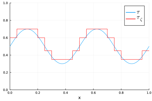
Figure 4.1: Example of a change interface $\tau$ and a piecewise constant approximation $\tau_{\zeta}$ in dimension $d=2$ with $\delta=0.05$.

Under Hölder smoothness assumptions on the change interface $\tau^{0}$, Theorem 3.7 allows us to obtain a convergence rate for the change domain estimator $\widehat{\Lambda}_{+}$ in the symmetric difference pseudometric, or equivalently, for the change interface estimator $\widehat{\tau}$ in the $L^{1}$-metric. For $\beta\in(0,1]$, $L>0$, let $\mathcal{H}(\beta,\mathsf{L})$ be the $(\beta,\mathsf{L})$-Hölder class on $[0,1]^{d-1}$ w.r.t. the maximum metric, i.e.,

$$\mathcal{H}(\beta,\mathsf{L})\coloneq\big{\{}f\colon[0,1]^{d-1}\to\operatorname{{\mathbb{R}}}:\lvert f(x)-f(y)\rvert\leq\mathsf{L}\lVert x-y\rVert_{\infty}^{\beta}\text{ for all }x,y\in[0,1]^{d-1}\big{\}}.$$

Proposition 4.1.

If $\tau^{0}\in\mathcal{H}(\beta,\mathsf{L})$ for $\beta\in(0,1]$ and $\mathsf{L}>0$, then there exists a constant $C$ depending only on $\beta,\mathsf{L},d,\underline{\vartheta},\overline{\vartheta},T$ and $\underline{\eta}$ such that

$$\operatorname{{\mathbb{E}}}\big{[}\lVert\widehat{\tau}-\tau^{0}\rVert_{L^{1}([0,1]^{d-1})}\big{]}=\operatorname{{\mathbb{E}}}\big{[}\bm{\lambda}(\widehat{\Lambda}_{+}\vartriangle\Lambda^{0}_{+})\big{]}\leq C\delta^{\beta}.$$

Moreover, if $\tau^{0}$ is not identically $1$ (resp. not identically $0$), then $\lvert\widehat{\vartheta}_{+}-\vartheta^{0}_{+}\rvert=\mathcal{O}_{\operatorname{{\mathbb{P}}}}(\delta^{\beta/2})$  (resp. $\lvert\widehat{\vartheta}_{-}-\vartheta^{0}_{-}\rvert=\mathcal{O}_{\operatorname{{\mathbb{P}}}}(\delta^{\beta/2})$). In particular, if $\tau^{0}(x)\in(0,1)$ for some $x\in[0,1]^{d-1}$, it holds that $\lVert\widehat{\vartheta}-\vartheta^{0}\rVert_{L^{1}((0,1)^{d})}\in\mathcal{O}_{\operatorname{{\mathbb{P}}}}(\delta^{\beta/2}).$

Proof.

By Theorem 3.7 and Corollary 3.10, it suffices to show that $\lvert\mathcal{B}\rvert\leq\mathsf{L}\delta^{d-\beta}$. To this end, we first observe that in the change interface model it holds that

$$\mathcal{B} =\big{\{}\alpha\in[n]^{d}:\operatorname{Sq}(\alpha)\cap\partial\Lambda^{0}_{+}\neq\varnothing\big{\}}$$

$$=\big{\{}(\gamma,j)\in[n]^{d-1}\times[n]:(\operatorname{Sq}_{d-1}(\gamma)^{\circ}\times((j-1)\delta,j\delta))\cap\tau^{0}(\operatorname{Sq}_{d-1}(\gamma))\neq\varnothing\big{\}}$$

$$\subset\big{\{}(\gamma,j)\in[n]^{d-1}\times[n]:j\in\delta^{-1}(\zeta^{\downarrow}_{\gamma},\zeta^{\uparrow}_{\gamma}]\big{\}}.$$

Because $\tau^{0}\in\mathcal{H}(\beta,\mathsf{L})$ implies that $\lvert\zeta^{\uparrow}_{\gamma}-\zeta^{\downarrow}_{\gamma}\rvert\leq\mathsf{L}\delta^{\beta}$ for any $\gamma\in[n]^{d-1}$, we obtain

$$\lvert\{j\in\delta^{-1}(\zeta^{\downarrow}_{\gamma},\zeta^{\uparrow}_{\gamma}]\cap[n]\}\rvert\leq\mathsf{L}\delta^{\beta-1}.$$

Thus, from above,

$$\lvert\mathcal{B}\rvert\leq\delta^{-(d-1)}\mathsf{L}\delta^{\beta-1}=\mathsf{L}\delta^{-d+\beta},$$

as desired. ∎

Remark 4.2.

The domain estimation rate $\delta^{\beta}$ translates to $N^{-\beta/d}$ in terms of the number of observations $N=\delta^{-d}$. As pointed out in [20, Chapter 3-5], for appropriately designed random measurement locations, the minimax rate for estimating a boundary fragment in image reconstruction is given by $N^{-\beta/(\beta+d-1)}$ for arbitrary $\beta>0$. Unless we have Lipschitz regularity $\beta=1$, this rate is, however, not achievable for an equidistant deterministic design, which is usually referred to as regular design. In fact, it can be shown that with regular design, the rate $N^{-\beta/d}$ is the optimal rate for $\beta\in(0,1]$ in the edge estimation problem by adapting [20, Theorem 3.3.1]. Indeed, consider the regular design image reconstruction problem

$$Y_{\alpha}=\vartheta(x_{\alpha})+\varepsilon_{\alpha},\quad\alpha\in[n]^{d},$$

where

$$\vartheta(x)=\vartheta_{-}\bm{1}_{\Lambda_{-}}(x)+\vartheta_{+}\bm{1}_{\Lambda_{+}}(x),\quad x\in[0,1]^{d},$$

for known values $\vartheta_{-}\neq\vartheta_{+}$ and $\Lambda_{-}\cupdot\Lambda_{+}=[0,1]^{d}$ and denote by $\operatorname{{\mathbb{P}}}_{\Lambda_{+}}$ the law generated by the observations for fixed $\Lambda_{+}$. Let $\tau^{0}\equiv 0$ and further let

$$\tau^{1}(x)\coloneq\sum_{\gamma\in[n]^{d-1}}\lVert x-z_{\gamma}\rVert_{\infty}^{\beta}\bm{1}_{\{\lVert x-z_{\gamma}\rVert_{\infty}\leq\delta/2\}},\quad x\in[0,1]^{d-1}.$$

Then, for $\Lambda_{+}^{i}\coloneq\{(x,y)\in[0,1]^{d}:\tau^{i}(x)>y\},$ $i=0,1$, we have

$$\{x_{\alpha}:\alpha\in[n]^{d}\}\subset\Lambda_{+}^{0}\cap\Lambda_{+}^{1}=\Lambda_{+}^{1},$$

and therefore $\operatorname{{\mathbb{P}}}_{\Lambda_{+}^{1}}=\operatorname{{\mathbb{P}}}_{\Lambda_{+}^{0}}$. Since furthermore $\bm{\lambda}(\Lambda_{+}^{0}\vartriangle\Lambda_{+}^{1})=\int\tau^{1}(x)\mathop{}\!\mathrm{d}{x}\asymp\delta^{\beta}$ and $\tau_{i}\in\mathcal{H}(\beta,1)$ for $i=0,1$, we obtain the minimax lower bound

$$\inf_{\widehat{\Lambda}_{+}}\sup_{\Lambda_{+}\in\Xi(\beta,\mathsf{L})}\operatorname{{\mathbb{E}}}_{\Lambda_{+}}\big{[}\bm{\lambda}(\widehat{\Lambda}_{+}\vartriangle\Lambda_{+})\big{]}\gtrsim\delta^{\beta}=N^{-\beta/d},$$

for the class $\Xi(\beta,\mathsf{L})$ of epigraphs of functions $\tau\in\mathcal{H}(\beta,1)$.

Remark 4.3.

Note that the underlying assumption on the graph orientation, that is $\Lambda^{0}_{+}$ is an epigraph w.r.t. the $d$-th coordinate, can be easily circumvented by adapting the candidate set $\mathcal{A}_{+}$ to represent any graph structure that may only become visible after rotation of the cube $[0,1]^{d}$. Since a $d$-dimensional hypercube admits $2d$ faces, the size of the adapted candidate set would increase from $n^{d-1}(n+1)$ to $2dn^{d-1}(n+1)$.

4.2 Estimation of convex sets

Suppose that model B from Section 2 holds, i.e., $\Lambda_{+}^{0}\subset\overline{\Lambda}$ is convex. A simple choice for $\mathcal{A}_{+}$ is given by $\mathcal{A}_{+}=\{C^{+}:C\subset[0,1]^{d}\text{ convex}\}$. This choice of candidate sets is however not particularly constructive. Let us therefore propose another family of candidate sets, whose construction follows a similar principle as the one for the graph representation model from the previous subsection.

The basic observation is that by convexity, for any $x\in\operatorname{int}\Lambda_{+}^{0}$, the vertical ray $y\mapsto x+ye_{d}$ intersects $\partial\Lambda_{+}$ in exactly two points. The natural idea is therefore to build candidate sets from hypercuboids $\operatorname{Sq}_{d-1}(\gamma)\times[\underline{\zeta}{}_{\gamma},\overline{\zeta}_{\gamma}]$ for $\underline{\zeta}_{\gamma},\overline{\zeta}_{\gamma}$ living on the grid $\mathcal{G}$. Heuristically speaking, as the upper and lower intersection points of the vertical ray can be described by a concave and convex function, respectively, we aim to approximate those by piecewise constant functions on $\widetilde{\operatorname{Sq}}_{d-1}(\gamma)$ in analogy to the graph representation of Section 4.1. In similarity to Section 4.1, let

$$\zeta^{\uparrow}_{\gamma} \coloneq\delta\lceil\delta^{-1}\sup\{x_{d}:x\in\partial\Lambda_{+}^{0}\cap(\operatorname{Sq}_{d-1}(\gamma)^{\circ}\times[0,1])\}\rceil,\quad\gamma\in[n]^{d-1},$$

$$\zeta^{\downarrow}_{\gamma} \coloneq\delta\lfloor\delta^{-1}\inf\{x_{d}:x\in\partial\Lambda_{+}^{0}\cap(\operatorname{Sq}_{d-1}(\gamma)^{\circ}\times[0,1])\}\rfloor,\quad\gamma\in[n]^{d-1},$$

be the grid projections of upper and lower limits of the intersection of the convex set $\Lambda^{+}_{0}$ with the strip $\operatorname{Sq}_{d-1}(\gamma)^{\circ}\times[0,1]$. Here, the supremum and the infimum of the empty is set to $0$. Consider candidate sets

$$\Lambda_{+}(\zeta)\coloneq\bigcup_{\gamma\in[n]^{d-1}:\underline{\zeta}_{\gamma}<\overline{\zeta}_{\gamma}}\operatorname{Sq}_{d-1}(\gamma)\times[\underline{\zeta}_{\gamma},\overline{\zeta}_{\gamma}],\quad\underline{\zeta}_{\gamma},\overline{\zeta}_{\gamma}\in\mathcal{G},$$

and the minimal tiling

$$\Lambda^{\updownarrow}_{+}\coloneq\bigcup_{\gamma\in[n]^{d-1}:\zeta_{\gamma}^{\downarrow}<\zeta_{\gamma}^{\uparrow}}\operatorname{Sq}_{d-1}(\gamma)\times[\zeta^{\downarrow}_{\gamma},\zeta^{\uparrow}_{\gamma}]$$

both belonging to

$$\mathcal{A}_{+}=\Big{\{}{\Lambda}_{+}(\zeta):\underline{\zeta}_{\gamma},\overline{\zeta}_{\gamma}\in\mathcal{G},\gamma\in[n]^{d-1}\Big{\}}.$$ (4.1)

Then, it holds that $\lvert\mathcal{A}_{+}\rvert=n^{d-1}((n+n^{2})/2+1)\asymp n^{d+1}$. An exemplary illustration in $d=2$ is given in Figure 4.2.

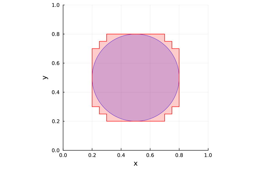
Figure 4.2: Approximation (red) of $\Lambda_{+}^{0}$ (blue) for $\delta=0.05.$; left: by some ${\Lambda}_{+}(\zeta)$ from (4.1); right: by $\Lambda_{+}^{\updownarrow}$.

In order to apply Theorem 3.7, it remains to control the size of the boundary tiling indices $\mathcal{B}$, which can be done with a classical result from convex geometry. By [22, Corollary 2], the boundary of any convex set $C\subset[0,1]^{d}$ can be covered by at most

$$n^{d}-(n-2)^{d}<2dn^{d-1}=2d\delta^{-d+1}$$

hypercubes from the tiling $\{\operatorname{Sq}(\alpha):\alpha\in[n]^{d}\}$ of $[0,1]^{d}$. This entails the bound

$$\lvert\mathcal{B}\rvert=\lvert\{\alpha\in[n]^{d}:\operatorname{Sq}(\alpha)^{\circ}\cap\partial\Lambda_{+}^{0}\neq\emptyset\}\rvert<2d\delta^{-d+1}.$$

Consequently, Theorem 3.7 and Corollary 3.10 yield the following convergence result.

Proposition 4.4.

Suppose that $\Lambda^{0}_{+}$ is convex and $\mathcal{A}_{+}$ be given by (4.1). Then, for some absolute constant $C$ depending only on $d,\underline{\vartheta},\overline{\vartheta},T$ and $\underline{\eta}$ it holds that

$$\operatorname{{\mathbb{E}}}\big{[}\bm{\lambda}(\widehat{\Lambda}_{+}\vartriangle\Lambda^{0}_{+})\big{]}\leq{C}\delta.$$

Moreover, if $\bm{\lambda}(\Lambda^{0}_{\pm})\neq 0$, it holds that $\lvert\widehat{\vartheta}_{\pm}-\vartheta^{0}_{\pm}\rvert\in\mathcal{O}_{\operatorname{{\mathbb{P}}}}(\delta^{1/2})$. In particular, if $\bm{\lambda}(\Lambda^{0}_{+})\notin\{0,1\}$, we have $\lVert\widehat{\vartheta}-\vartheta^{0}\rVert_{L^{1}((0,1)^{d}})\in\mathcal{O}_{\operatorname{{\mathbb{P}}}}(\delta^{1/2})$.

Remark 4.5.

For an indication of optimality of the domain convergence rate, let us again consider the regular design image reconstruction problem

$$Y_{\alpha}=\vartheta(x_{\alpha})+\varepsilon_{\alpha},\quad\alpha\in[n]^{d},$$

from Remark 4.2. Let $\Lambda_{+}^{0}\subset(0,1)^{d}$ be an open hypercube with volume $v_{0}\in(0,1)$ and edge length $l_{0}=v_{0}^{1/d}$ such that the corners of the hypercube lie on $\{x_{\alpha}\}_{\alpha\in[n]^{d}}$ and let $\Lambda^{1}_{+}$ be the open hypercube containing $\Lambda^{0}_{+}$ such that $d_{\infty}(\Lambda_{+}^{0},\Lambda_{+}^{1})=\delta/2$, where $\delta$ is chosen small enough s.t. $\Lambda_{+}\subset(0,1)^{d}$. Then $x_{\alpha}\in\Lambda_{0}^{+}$ iff $x_{\alpha}\in\Lambda_{+}^{0}$ and therefore $\operatorname{{\mathbb{P}}}_{\Lambda_{+}^{0}}=\operatorname{{\mathbb{P}}}_{\Lambda_{+}^{1}}$. Moreover,

$$\bm{\lambda}(\Lambda_{+}^{0}\vartriangle\Lambda^{1}_{+})=(l_{0}+\delta/2)^{d}-l_{0}^{d}\geq\frac{d}{2}l_{0}^{d-1}\delta=\delta\frac{d}{2}v_{0}^{\frac{d-1}{d}},$$

yielding the minimax lower bound

$$\inf_{\widehat{\Lambda}_{+}}\sup_{\Lambda_{+}\in\mathcal{C}(v_{0})}\operatorname{{\mathbb{E}}}_{\Lambda_{+}}\big{[}\bm{\lambda}(\widehat{\Lambda}_{+}\vartriangle\Lambda_{+})\big{]}\gtrsim C(v_{0})\delta,$$

for the class $\mathcal{C}(v_{0})$ of convex sets in $[0,1]^{d}$ with volume at least $v_{0}\in(0,1)$.

The constructed estimator $\widehat{\Lambda}_{+}$ has the drawback of generally not being a convex or even connected set. However, we can easily transform our estimator $\widehat{\Lambda}_{+}$ into a convex estimator $\widehat{\Lambda}{}^{\mathrm{con}}_{+}$ that converges at the same rate. To this end we employ a minimum distance fit by choosing an estimator $\widehat{\Lambda}{}^{\mathrm{con}}_{+}$ such that

$$\bm{\lambda}\big{(}\widehat{\Lambda}{}^{\mathrm{con}}_{+}\vartriangle\widehat{\Lambda}_{+}\big{)}\leq\inf_{C\subset[0,1]^{d}:C\text{ is convex}}\bm{\lambda}\big{(}C\vartriangle\widehat{\Lambda}_{+}\big{)}+\delta.$$

Up to a $\delta$-margin, $\widehat{\Lambda}^{\mathrm{con}}_{+}$ is therefore a convex set with maximal overlap in volume with $\widehat{\Lambda}_{+}$.

Corollary 4.6.

The convex estimator $\widehat{\Lambda}{}^{\mathrm{con}}_{+}$ satisfies

$$\operatorname{{\mathbb{E}}}\big{[}\bm{\lambda}(\widehat{\Lambda}{}^{\mathrm{con}}_{+}\vartriangle\Lambda^{0}_{+})\big{]}\leq(2C+1)\delta,$$

where $C$ is the constant from Proposition 4.4.

Proof.

By triangle inequality for the symmetric difference pseudometric, it follows that

$$\operatorname{{\mathbb{E}}}\big{[}\bm{\lambda}\big{(}\Lambda_{+}^{0}\vartriangle\widehat{\Lambda}{}^{\mathrm{con}}_{+}\big{)}\big{]} \leq\operatorname{{\mathbb{E}}}\big{[}\bm{\lambda}\big{(}\widehat{\Lambda}{}^{\mathrm{con}}_{+}\vartriangle\widehat{\Lambda}_{+}\big{)}\big{]}+\operatorname{{\mathbb{E}}}\big{[}\bm{\lambda}\big{(}\Lambda_{+}^{0}\vartriangle\widehat{\Lambda}_{+}\big{)}\big{]}$$

$$\leq 2\operatorname{{\mathbb{E}}}\big{[}\bm{\lambda}\big{(}\Lambda_{+}^{0}\vartriangle\widehat{\Lambda}_{+}\big{)}\big{]}+\delta,$$

where we used that

$$\bm{\lambda}\big{(}\widehat{\Lambda}{}^{\mathrm{con}}_{+}\vartriangle\widehat{\Lambda}_{+}\big{)}\leq\bm{\lambda}\big{(}\Lambda_{+}^{0}\vartriangle\widehat{\Lambda}_{+}\big{)}+\delta$$

since $\Lambda_{+}^{0}$ is convex. The assertion therefore follows from Proposition 4.4. ∎

Given the estimator $\widehat{\Lambda}_{+}$, numerical implementation of $\widehat{\Lambda}^{\mathrm{con}}_{+}$ can be conducted with methods for convexity constrained image segmentation based on the binary image input $\{(x_{\alpha},\bm{1}_{\widehat{\Lambda}_{+}}(x_{\alpha})):\alpha\in[n]^{d}\}$, see, e.g., the recent implicit representation approach in [33].

5 Conclusion and outlook

Before discussing limitations and possible extensions of our work, let us briefly summarize our results. We have studied a change estimation problem for a stochastic heat equation (1.1) in $d\geq 2.$ The underlying space is partitioned into $\Lambda_{-}\cup\Lambda_{+}$ by a separating hypersurface $\Gamma=\partial\Lambda_{+}$, where the piecewise constant diffusivity $\vartheta$ exhibits a jump. Following a CUSUM approach, we have constructed an M-estimator $\widehat{\Lambda}_{+}$ based on local measurements on a fixed uniform $\delta$-grid that exhibits certain analogies to regular design estimators in statistical image reconstruction. Our main result, Theorem 3.7, shows how the convergence properties of our estimator are determined by the number of tiles that are sliced by $\Gamma$. The estimation principle and rates are made concrete for two specific models that impose shape restrictions on the change domain $\Lambda_{+}$: (A) a graph representation of $\Gamma$ with Hölder smoothness $\beta\in(0,1],$ and (B) a convex shape. We have established the rates of convergences $\delta^{\beta}$ for model A and $\delta$ for model B with respect to the symmetric difference risk $\operatorname{{\mathbb{E}}}[\bm{\lambda}(\widehat{\Lambda}_{+}\vartriangle\Lambda_{+})]$, which are the optimal rates of convergence in the corresponding image reconstruction problems with regular design. Furthermore, the diffusivity parameters can be recovered with rate $\delta^{\beta/2}$ and $\delta^{1/2}$. To conclude the paper, let us now give an outlook on potential future work that can build on our results.

Based on Theorem 3.7, an extension of Proposition 4.1 to a known number $m$ of change interfaces $\tau_{1},\dots,\tau_{m}$ that yields a partition $\overline{\Lambda}=\bigcup_{0\leq i\leq m}\Lambda_{i}$ of layers $\Lambda_{i}$ with alternating diffusivities $\vartheta_{\pm}$, is straightforward. Assuming that each $\tau_{m}$ belongs to $\mathcal{H}(\beta,L)$, the same rate of convergence can be established. For the canonical choice $\mathcal{A}_{+}=\mathcal{P}$, our general estimator from Theorem 3.7 would also adapt to an unknown number of layers $m$, but it might be interesting in this scenario to develop a more implementation friendly procedure.

Having an unknown number of layers, or, more generally, an unknown number of “impurities” is also particularly interesting from a testing perspective. In this spirit, a further model extension would allow a partition $\overline{\Lambda}=\bigcup_{0\leq i\leq m}\Lambda_{i}$ with $\vartheta\equiv\vartheta_{i}$ on $\Lambda_{i}$ and $\vartheta_{i}\neq\vartheta_{j}$ for $j\neq i$, which can be used, for instance, to model sediment layers. This model extension is unproblematic from an SPDE perspective, but poses additional statistical challenges.

More generally, besides spatial change areas, future work could contain temporal change points, i.e., the diffusivity $\vartheta=\vartheta(t,x)$ is also discontinuous in time, thereby allowing for the modeling of thermal spikes. In this case, tools from change point detection in time series have to be incorporated into the estimation procedure and online estimation becomes an intriguing question.

In this paper, we have fixed the parameters $\vartheta_{\pm}$ and therefore also the absolute jump height $\eta=\lvert\vartheta_{+}-\vartheta_{-}\rvert$. Extensions of the result to a $\delta$-dependent, but non-vanishing jump height, i.e., $\eta=\eta(\delta)\geq\underline{\eta}$ for some fixed $\underline{\eta}>0$, are straightforward. In contrast, the vanishing jump height regime $\eta\to 0$ as $\delta\to 0$ that has been considered for the one-dimensional change point problem in [30], introduces significant technical challenges that require a sharper concentration analysis. Similarly to how the limit result from [30] in this regime draws analogies to classical change point limit theorems, in our multivariate case one would expect asymptotics that are comparable to [25].

As mentioned in Remark 4.2 and Remark 4.5, the convergence rates for $N^{-\beta/d}$ and $N^{-1/d}$, respectively, are optimal in the related image reconstruction problem when working with a regular design. However, as alluded to before, it is shown in [20] that the minimax optimal rate for irregular measurement designs that introduce a certain level of randomness is given by $N^{-\beta/(\beta+d-1)}$ for arbitrary $\beta>0$, which is not only substantially faster for $\beta\in(0,1)$, but also allows to exploit higher-order smoothness of the change interface. Appropriately introducing such randomness in the measurement locations $x_{\alpha}$ of the local observation scheme while preserving favorable probabilistic properties such as independence of the associated Brownian motions $B_{\delta,\alpha}$ is a conceptually challenging task that could contribute to improve change domain estimation performance in the given heat equation model.

Finally, let us reiterate that we have focused on optimal change domain estimation for regular local measurements and have not attempted to optimize estimation rates for the diffusivity parameters $\vartheta_{\pm}$. For the binary image reconstruction model with regeression function $\vartheta(x)=\vartheta_{+}\bm{1}_{\Lambda_{+}}(x)+\vartheta_{-}\bm{1}_{\Lambda_{-}}(x),$ [20, Theorem 5.1.2] establishes the typical parametric rate $N^{-1/2}=\delta^{d/2}$ for $\vartheta_{\pm}$. On the other hand, [5] prove the minimax rate $\delta^{d/2+1}$ for a constant diffusivity, which can also be obtained in the one-dimensional change point estimation problem for a stochastic heat equation by introducing an additional nuisance parameter $\vartheta_{\circ}$ in the estimation procedure that reduces the bias from a constant approximation $\vartheta\equiv\vartheta_{\circ}$ on a proposed spatial change interval, cf. [30, Theorem 3.12]. This demonstrates a significant difference between heat diffusivity and image estimation. Optimal diffusivity estimation in the here considered change estimation problem is therefore an especially relevant task for future work, which may also open the door to the investigation of fully nonparametric diffusivities $\vartheta(x)=\vartheta_{-}(x)\bm{1}_{\Lambda_{-}}(x)+\vartheta_{+}(x)\bm{1}_{\Lambda_{+}}(x)$.

Acknowledgements

The authors gratefully acknowledge financial support of Carlsberg Foundation Young Researcher Fellowship grant CF20-0640 “Exploring the potential of nonparametric modelling of complex systems via SPDEs”.

References

- [1] Randolf Altmeyer, Till Bretschneider, Josef Janák and Markus Reiß “Parameter Estimation in an SPDE Model for Cell Repolarisation” In SIAM/ASA J. Uncertain. Quantif. 10.1, 2022, pp. 179–199
- [2] Randolf Altmeyer, Igor Cialenco and Gregor Pasemann “Parameter estimation for semilinear SPDEs from local measurements” In Bernoulli 29.3 Bernoulli Society for Mathematical StatisticsProbability, 2023, pp. 2035 –2061 DOI: 10.3150/22-BEJ1531
- [3] Randolf Altmeyer, Igor Cialenco and Markus Reiß “Statistics for SPDEs” Accessed: 2024-04-29, https://sites.google.com/view/stats4spdes
- [4] Randolf Altmeyer and Markus Reiss “Nonparametric estimation for linear SPDEs from local measurements” In Ann. Appl. Probab. 31.1, 2021, pp. 1–38 DOI: 10.1214/20-aap1581
- [5] Randolf Altmeyer, Anton Tiepner and Martin Wahl “Optimal parameter estimation for linear SPDEs from multiple measurements” In Ann. Statist., to appear arXiv:2211.02496 [math.ST]
- [6] Christopher J. Bishop and Yuval Peres “Fractals in probability and analysis” 162, Cambridge Studies in Advanced Mathematics Cambridge University Press, Cambridge, 2017, pp. ix+402 DOI: 10.1017/9781316460238
- [7] Carsten Chong “High-frequency analysis of parabolic stochastic PDEs” In Ann. Stat. 48.2, 2020, pp. 1143–1167 URL: https://arxiv.org/abs/1806.06959
- [8] Igor Cialenco “Statistical inference for SPDEs: an overview” In Stat. Inference Stoch. Process. 21.2, 2018, pp. 309–329 DOI: 10.1007/s11203-018-9177-9
- [9] Igor Cialenco, Francisco Delgado-Vences and Hyun-Jung Kim “Drift Estimation for Discretely Sampled SPDEs” In Stoch. Partial Differ. Equ. Anal. Comput. 8, 2020, pp. 895–920 URL: https://arxiv.org/abs/1904.10884v1
- [10] Igor Cialenco, Sergey V Lototsky and Jan Pospíšil “Asymptotic properties of the maximum likelihood estimator for stochastic parabolic equations with additive fractional Brownian motion” In Stoch. Dyn. 9.02, 2009, pp. 169–185
- [11] Giuseppe Da Prato and Jerzy Zabczyk “Stochastic equations in infinite dimensions” Cambridge University Press, 2014
- [12] E. B. Davies “Heat kernels and spectral theory” 92, Cambridge Tracts in Mathematics Cambridge University Press, 1990
- [13] E. B. Davies “Spectral theory and differential operators” 42, Cambridge Studies in Advanced Mathematics Cambridge University Press, 1995 DOI: 10.1017/CBO9780511623721
- [14] Florian Hildebrandt and Mathias Trabs “Parameter estimation for SPDEs based on discrete observations in time and space.” In Electron. J. Stat. 15, 2021, pp. 2716–2776 URL: https://arxiv.org/abs/2001.03403v1
- [15] Marianne Huebner and Boris Rozovskii “On asymptotic properties of maximum likelihood estimators for parabolic stochastic PDE’s” In Probab. Theory Related Fields 103.2, 1995, pp. 143–163 DOI: 10.1007/BF01204212
- [16] Josef Janák and Markus Reiß “Parameter estimation for the stochastic heat equation with multiplicative noise from local measurements” In Stochastic Process. Appl. 175, 2024, pp. Paper No. 104385 DOI: 10.1016/j.spa.2024.104385
- [17] Yusuke Kaino and Masayuki Uchida “Parametric estimation for a parabolic linear SPDE model based on discrete observations” In J. Statist. Plann. Inference 211, 2021, pp. 190–220 DOI: 10.1016/j.jspi.2020.05.004
- [18] A. P. Korostelëv, L. Simar and A. B. Tsybakov “Efficient estimation of monotone boundaries” In Ann. Statist. 23.2, 1995, pp. 476–489 DOI: 10.1214/aos/1176324531
- [19] A. P. Korostelev, L. Simar and A. B. Tsybakov “On estimation of monotone and convex boundaries” In Publ. Inst. Statist. Univ. Paris 39.1, 1995, pp. 3–18
- [20] A. P. Korostelëv and A. B. Tsybakov “Minimax theory of image reconstruction” 82, Lecture Notes in Statistics Springer, 1993 DOI: 10.1007/978-1-4612-2712-0
- [21] Charu Krishnamoorthy and Ed Carlstein “Practical Considerations in Boundary Estimation: Model-Robustness, Efficient Computation, and Bootstrapping” In Lecture Notes-Monograph Series 23 Institute of Mathematical Statistics, 1994, pp. 177–193 URL: http://www.jstor.org/stable/4355773
- [22] Marek Lassak “Covering the Boundary of a Convex Set by Tiles” In Proc. Amer. Math. Soc. 104.1 American Mathematical Society, 1988, pp. 269–272 URL: http://www.jstor.org/stable/2047500
- [23] W Liu and S. Lototsky “Parameter estimation in hyperbolic multichannel models” In Asymptot. Anal. 68, 2010 DOI: 10.3233/ASY-2010-0992
- [24] Sergey V. Lototsky “Parameter Estimation for Stochastic Parabolic Equations: Asymptotic Properties of a Two-Dimensional Projection-Based Estimator” In Stat. Inference Stoch. Process. 6.1, 2003, pp. 65–87 DOI: 10.1023/A:1022699622088
- [25] H. G. Müller and K.-S. Song “A set-indexed process in a two-region image” In Stochastic Process. Appl. 62, 1996, pp. 87–101
- [26] H. G. Müller and K.-S. Song “Cube Splitting in Multidimensional Edge Estimation” In Lecture Notes-Monograph Series 23 Institute of Mathematical Statistics, 1994, pp. 210–223 URL: http://www.jstor.org/stable/4355775
- [27] H. G. Müller and K.-S. Song “Maximin estimation of multidimensional boundaries” In J. Multivariate Anal. 50.2, 1994, pp. 265–281
- [28] Gregor Pasemann and Wilhelm Stannat “Drift estimation for stochastic reaction-diffusion systems” In Electron. J. Stat. 14.1, 2020, pp. 547–579 DOI: 10.1214/19-ejs1665
- [29] Peihua Qiu “Jump Surface Estimation, Edge Detection, and Image Restoration” In J. Amer. Statist. Assoc. 102.478 Taylor & Francis, 2007, pp. 745–756 DOI: 10.1198/016214507000000301
- [30] Markus Reiß, Claudia Strauch and Lukas Trottner “Change point estimation for a stochastic heat equation”, 2023 arXiv:2307.10960 [math.ST]
- [31] Mats Rudemo and Henrik Stryhn “Approximating the Distribution of Maximum Likelihood Contour Estimators in Two-Region Images” In Scand. J. Stat. 21.1 [Board of the Foundation of the Scandinavian Journal of Statistics, Wiley], 1994, pp. 41–55 URL: http://www.jstor.org/stable/4616297
- [32] Mats Rudemo and Henrik Stryhn “Boundary Estimation for Star-Shaped Objects” In Lecture Notes-Monograph Series 23 Institute of Mathematical Statistics, 1994, pp. 276–283 URL: http://www.jstor.org/stable/4355779
- [33] Jan Philipp Schneider, Mishal Fatima, Jovita Lukasik, Andreas Kolb, Margret Keuper and Michael Moeller “Implicit Representations for Constrained Image Segmentation” In Proceedings of the 41st International Conference on Machine Learning 235, Proceedings of Machine Learning Research PMLR, 2024, pp. 43765–43790 URL: https://proceedings.mlr.press/v235/schneider24a.html
- [34] Claudia Strauch and Anton Tiepner “Nonparametric velocity estimation in stochastic convection-diffusion equations from multiple local measurements”, 2024 arXiv:2402.08353 [math.ST]
- [35] Yozo Tonaki, Yusuke Kaino and Masayuki Uchida “Parameter estimation for linear parabolic SPDEs in two space dimensions based on high frequency data” In Scand. J. Stat. 50.4, 2023, pp. 1568–1589 DOI: https://doi.org/10.1111/sjos.12663
- [36] A. B. Tsybakov “Multidimensional change-point problems and boundary estimation” In Change-point problems (South Hadley, MA, 1992) 23, IMS Lecture Notes Monogr. Ser. Inst. Math. Statist., Hayward, CA, 1994, pp. 317–329 DOI: 10.1214/lnms/1215463133
- [37] Eric Ziebell “Non-parametric estimation for the stochastic wave equation”, 2024 arXiv:2404.18823 [math.ST]