Efficient Large-Scale Quantum Optimization via Counterdiabatic Ansatz
Abstract
Quantum Approximate Optimization Algorithm (QAOA) is one of the fundamental variational quantum algorithms, while a version of QAOA that includes counterdiabatic driving, termed Digitized Counterdiabatic QAOA (DC-QAOA), is generally considered to outperform QAOA for all system sizes when the circuit depth for the two algorithms are held equal. Nevertheless, DC-QAOA introduces more CNOT gates per layer, so the overall circuit complexity is a tradeoff between the number of CNOT gates per layer and the circuit depth, and must therefore be carefully assessed. In this paper, we conduct a comprehensive comparison of DC-QAOA and QAOA on MaxCut problem with the total number of CNOT gates held equal, and we focus on one implementation of counterdiabatic terms using nested commutators in DC-QAOA, termed as DC-QAOA(NC). We have found that DC-QAOA(NC) reduces the overall circuit complexity as compared to QAOA only for sufficiently large problems, and for MaxCut problem the number of qubits must exceed 16 for DC-QAOA(NC) to outperform QAOA. We have further shown that this advantage can be understood from the effective dimensions introduced by the counterdiabatic driving terms. Moreover, based on our finding that the optimal parameters generated by DC-QAOA(NC) strongly concentrate in the parameter space, we haved devised an instance-sequential training method for DC-QAOA(NC) circuits, which, compared to traditional methods, offers performance improvement while using even fewer quantum resources. Our findings provide a more comprehensive understanding of the advantages of DC-QAOA circuits and an efficient training method based on their generalizability.
I INTRODUCTION
Variational Quantum Algorithms (VQAs) provide an efficient way to tackle complex problems by merging classical optimization techniques with quantum computing circuits Cerezo et al. (2021); Kandala et al. (2017); Mitarai et al. (2018); McClean et al. (2016); Liu et al. (2019); Peruzzo et al. (2014); Haug et al. (2021); Abbas et al. (2021). Inspired by adiabatic quantum processes Comparat (2009), the Quantum Approximate Optimization Algorithm (QAOA) is a type of VQA particularly suited for combinatorial optimization problems Hadfield et al. (2019); Zhou et al. (2020, 2023). QAOA constructs a parametrized quantum circuit (“ansatz”) composed of alternating layers of problem-specific cost functions (encoded as quantum operators) and mixing unitary operations. These parameters are then optimized iteratively using classical optimization methods to approach optimal solutions to a given problem. The capability of QAOA to handle a wide array of optimization problems, including MaxCut, Graph Partitioning, and others, underscores its significance in quantum computing Zhu et al. (2022); Ruan et al. (2023); Oh et al. (2019).
In principle, QAOA becomes more powerful as the number of layers increases Farhi et al. (2014). However, its implementation is challenging for current Noisy Intermediate-Scale Quantum (NISQ) devices due to their limited coherence times. On the other hand, adiabatic quantum processes can be accelerated by adding counterdiabatic terms (cd-terms), known as counterdiabatic driving (cd-driving) in Shortcut to Adiabaticity (STA) Chen et al. (2010); Vacanti et al. (2014); Ji et al. (2022); Hartmann and Lechner (2019). It has been demonstrated that, under certain situations, the performance of QAOA can be enhanced by incorporating cd-terms in a digitized fashion, resulting in the Digitized Counterdiabatic Quantum Approximate Optimization Algorithm (DC-QAOA) Hegade et al. (2021); Chandarana et al. (2022).
Recent studies have compared the performance of DC-QAOA and QAOA in a variety of problems, including ground state preparation Chandarana et al. (2022), molecular docking Ding et al. (2024), protein folding Chandarana et al. (2023), and portfolio optimization Hegade et al. (2022). In all these studies, the comparisons were made when both algorithms have the same number of circuit layers. The fact that DC-QAOA exhibits an advantage over QAOA in these studies suggests that cd-terms effectively reduce the number of circuit layers required to achieve the same level of efficiency. Nevertheless, the circuit complexity for a NISQ device, which is directly linked to the execution time, depends not only on the number of layers but also the number of two-qubit gates in each layer. While reducing the number of layers required by DC-QAOA to achieve the same efficiency as QAOA, cd-terms introduce more two-qubit gates, substantially complicating the circuit. Therefore, apart from the number of layers considered in the literature, the number of two-qubit gates is also playing a key role in comparing the performances between DC-QAOA and QAOA on actual NISQ devices.
In this paper, we compare DC-QAOA and QAOA on the MaxCut problem Aoshima and Iri (1977), where the number of layers is increased until both algorithms reach the predefined fidelity to the ground state of optimization problems. We use the number of CNOT gates as an indicator of efficiency since it characterizes the difficulty of implementing such algorithms on quantum computers. Using MaxCut on randomly generated unweighted graphs as benchmarks, we found that for graphs with over 16 vertices, DC-QAOA can achieve better performance using fewer two-qubit gates, while QAOA is better for smaller graphs. By closely examining the effective dimension of the two circuits, we find that adding cd-terms in each layer provides more effective dimensions than simply adding more layers to QAOA, and the cd-terms can suppress non-diagonal transitions, thereby improving DC-QAOA’s performance. Furthermore, the optimal parameters obtained by training DC-QAOA display a strong concentration in the parameter space, demonstrating potential transferability and generalizability from optimization problems on a smaller scale to those on a larger scale. Based on our findings, we devised an Instance-Sequential Training (IST) method for DC-QAOA, which enables comparable or superior outcomes with substantially reduced quantum resources. As a result, DC-QAOA emerges as a more viable option for extensive quantum optimization tasks, in contrast to QAOA, which may be more efficient for smaller-scale problems.
The remainder of the paper is organized as follows. In Section II, we introduce the formalism including definitions of QAOA and DC-QAOA. Section III provides the results. We show a comprehensive comparision of DC-QAOA and QAOA in Section III.1. In Section III.2, we discuss how DC-QAOA benefits from cd-terms, and in Section III.3, we demonstrate the parameter concentration phenomenon in DC-QAOA and propose a quantum resource-efficient training method. We conclude in Section IV.
II Formalism
QAOA can be seen as a digitized version of Adiabatic Quantum Computing with trainable parameters Barends et al. (2016). The ansatz of QAOA stems from the quantum annealing Hamiltonian:
| (1) |
where is the annealing schedule in . As , the ground state of can evolve adiabatically into the ground state of . Here, , allowing the ground state of to be easily prepared as an equally weighted superposition state in the computational bases, and can be any Hamiltonian of interest. Quantum annealing can be digitized with trotterized time evolution:
| (2) |
Here, is the number of trotter layers, and when is sufficiently large, approaches the adiabatic limit. can be further parameterized with a set of trainable parameters instead of original annealing schedule to counter coherent errors in NISQ devices:
| (3) |
where the unitary operators are and . By maximizing an objective function , defined below in Eq. (7) for the MaxCut problem, we minimize the distance between the output state and the exact ground state of . Hence adiabatic quantum evolution is transformed into an optimization problem with parameters.
However, the requirement for a large number of trotter layers in QAOA to approximate adiabatic evolution poses challenges due to the increased circuit complexity. To address this limitation, DC-QAOA has been developed Chandarana et al. (2022). DC-QAOA builds upon analog cd-driving which can shorten the evolution time of adiabatic transitions by adding an extra cd-term, presenting an opportunity to effectively reduce number of layers in QAOA. The nature of the cd-terms depends on the choice of appropriate adiabatic gauge potential Sels and Polkovnikov (2017). In the realm of analog cd-driving, the commonly utilized gauge potential is first-order nested commutators
| (4) |
In cd-driving, the effective Hamiltonian can be written as
| (5) |
Following the same routine in QAOA, cd-driving can be similarly digitized and parameterized as
| (6) |
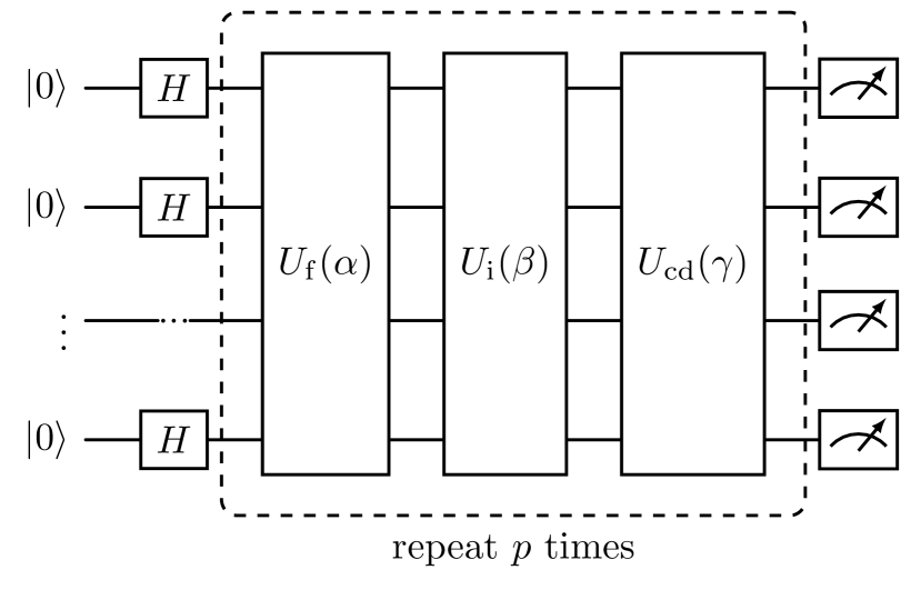
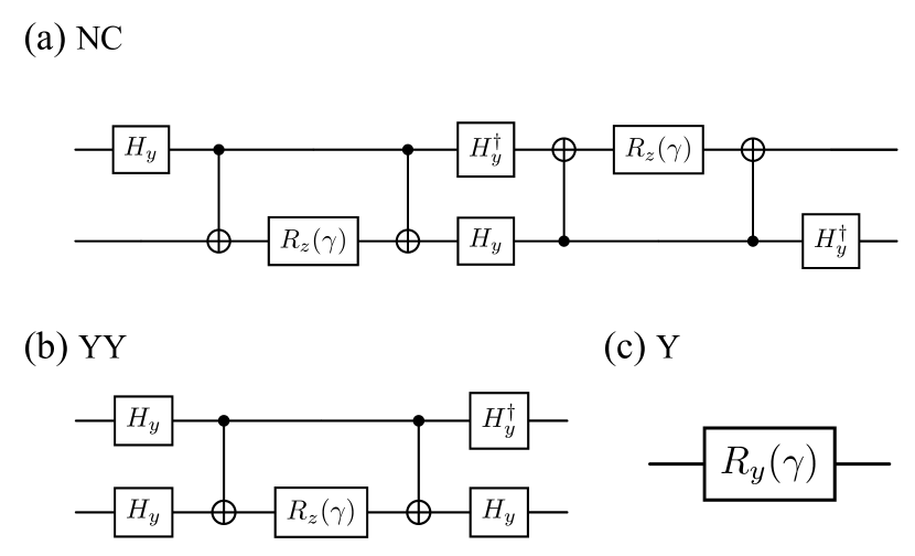
A schematic circuit diagram of a typical -layer DC-QAOA is shown in Fig. 1. The detailed implementation of three possible cd-terms in DC-QAOA using elementary gates, including first-order nested commutator (hereafter referred to as NC) Chandarana et al. (2023), single qubit Y-rotation (referred to as Y) Čepaitė et al. (2023), and two-qubit YY-Interaction (referred to as YY) Chai et al. (2022), can be seen in Fig. 2. In this paper, we denote the three versions of the DC-QAOA algorithm which uses NC, YY and Y as cd-terms as DC-QAOA(NC), DC-QAOA(YY), and DC-QAOA(Y), respectively.
To explore the advantage of DC-QAOA over QAOA on quantum optimization problems, we use the MaxCut problem as a benchmark Goemans and Williamson (1995). For the MaxCut problems with an unweighted graph , where and are the vertex and edge sets respectively, the objective function is defined on a string of binary values :
| (7) |
which aims to separate the vertices into two subsets so that is maximized. Depending on which subset vertex is in, is assigned a binary value of 0 or 1. The solution is embedded in the ground state of , written as
| (8) |
By finding the ground state of , we can maximize the objective function .
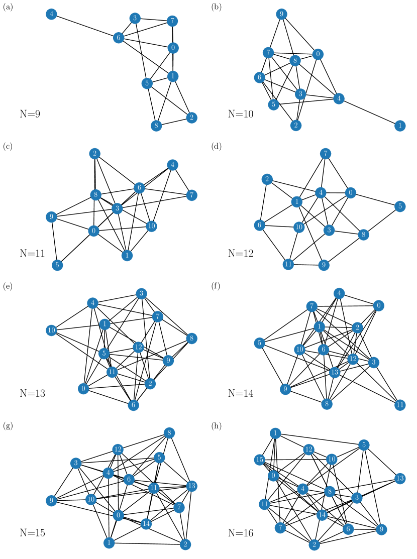
In this study, for each given number of vertices between 9 and 16, we randomly generate one graph, subject to the condition that the edges between every pair of vertices are connected with probability . These graphs are shown in the Appendix.
III RESULTS
III.1 Circuit Length Scaling Behavior
In the current literature, the comparison between DC-QAOA and QAOA is done holding the number of layers equal, under which condition it has been claimed that DC-QAOA has superior performance than QAOA in quantum optimization for essentially systems of any size Chandarana et al. (2022, 2023). However, from Eq. (3) and Eq. (6) we can see that DC-QAOA adds a cd-term to every layer of QAOA. The inclusion of cd-terms in DC-QAOA brings about an inherent trade-off, adding two-qubit gates to the quantum circuit, thereby heightening the circuit complexity even when the number of layers remains the same as in QAOA. The effect is even more pronounced for NISQ devices due to their decoherence and limited connectivity among qubits.
For a MaxCut problem on graph having edges, the implementation of requires CNOT gates, and the implementation of requires , and CNOT gates for NC (Fig. 2(a)), YY (Fig. 2(b)) and Y (Fig. 2(c)), respectively. Note that QAOA has CNOT gates, therefore DC-QAOA(NC), DC-QAOA(YY), and DC-QAOA(Y) has , , and CNOT gates in total respectively. It is worth noting that DC-QAOA(NC) utilizes three times CNOT gates as in QAOA, the most among the three versions of the algorithm.
It has been found that the depth of QAOA required to reach the ground state of Hamiltonian with a predefined fixed probability scales roughly linearly with problem size Akshay et al. (2022). Such depth is called the critical depth, denoted as , which provides a tool to quantify the advantage afforded by adding cd-terms in DC-QAOA. It is important to see how fast scales with problem size. For example, if of DC-QAOA(NC) scales three times slower than of QAOA, it means that as the problem size grows, DC-QAOA(NC) can eventually solve an optimization problem utilizing fewer CNOT gates than QAOA. Therefore, it is fair to compare DC-QAOA and QAOA by comparing the scaling rate of versus the problem size. To find the critical depth for DC-QAOA and QAOA, we first define the approximate ratio :
| (9) |
which is the fidelity between the output state of the quantum algorithm and the ground state of . Then, we determine the critical depth as the minimum number of layers required in DC-QAOA or QAOA for to exceed 90%.
Fig. 3 shows the approximate ratio , calculated at fixed number of layers , for a MaxCut problem with 16 vertices (cf. Fig. 9(h)) versus number of training iterations for four different versions of the algorithms. Different algorithms converge to different values of , with a higher value indicating a better performance. Each panel shows eight color lines, which are 8 runs from random initialization of parameters. The converged value of for different algorithms are averaged and are shown in Table 1. Overall, the results from DC-QAOA(NC) (Fig. 3(b)) is the best, followed by those from DC-QAOA(YY) (Fig. 3(c)). Results from DC-QAOA(Y) (Fig. 3(d)) and QAOA (Fig. 3(a)) are comparable and are both inferior to the other two methods. These results suggest having more CNOT gates on each layer implies better performance of the algorithm.
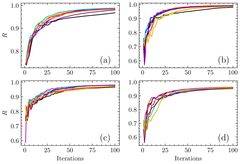
| Algorithm | Mean | Std. |
|---|---|---|
| QAOA | 97.85% | 0.65% |
| DC-QAOA(NC) | 98.87% | 0.38% |
| DC-QAOA(YY) | 98.62% | 0.51% |
| DC-QAOA(Y) | 98.30% | 0.40% |
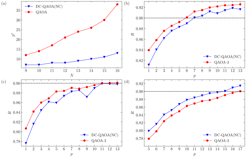
To elucidate how the combined effect of the number of CNOT gates and number of layers on the effectiveness of the algorithm, we focus on comparing DC-QAOA(NC), which has the most number of CNOT gates per layer, to QAOA. In Fig. 4(a) we compare the critical depth as functions of the number of qubits , for both QAOA and DC-QAOA(NC). The calculated critical depths for both algorithms scale approximately linearly with system size as (for QAOA) and (for DC-QAOA(NC)). Therefore, in the limit of solving large scale MaxCut problem on graph with edges, QAOA needs layers and in turn CNOT gates and DC-QAOA(NC) needs layers and in turn CNOT gates. This implies that DC-QAOA(NC) is more advantageous than QAOA in solving large scale optimization problem because the total number of CNOT gates required to achieve the same level of effectiveness is smaller for DC-QAOA(NC), when is sufficiently large. In other words, the circuit complexity for DC-QAOA(NC) is lower, taking into consideration both the number of effective layers and the number of CNOT gates per layer required.
We set and obtain . This suggests that DC-QAOA(NC) is more advantageous than QAOA when the number of vertices exceeds 16 (i.e. ). To show this more clearly, we execute DC-QAOA(NC) with layers, and a QAOA with intentionaly-set layers (which is denoted as QAOA-3 in Fig. 4(b),(c) and (d) and should not be confused with regular QAOA with layers), to solve the MaxCut problem with different number of vertices. Fig. 4(b) shows the results on 12 vertices (cf. Fig. 9(d)), and one can see that QAOA-3 clearly performs better than DC-QAOA(NC). Fig. 4(c) shows the results on 16 vertices (cf. Fig. 9(h)), in which situation the two algorithms are comparable. Given that is still less than 16.94, it is reasonable that QAOA-3 outperforms DC-QAOA(NC) slightly at this stage, although DC-QAOA(NC) rapidly approaches similar performance with increasing . When , the difference in between DC-QAOA(NC) and QAOA becomes negligible. We have also conducted a calculation comparing QAOA-3 and DC-QAOA(NC) for a problem with 20 vertices, with results shown in Fig. 4 (d), although the calculation is more expensive. In this case, DC-QAOA(NC) is clearly superior than QAQA-3. Our results shown in Fig. 4 confirms that DC-QAOA(NC) is only more advantageous than QAOA on graphs with more than 16 vertices. To our knowledge, this fact has not been noted in the literature and is the key result of this paper.
III.2 Effective Dimension and Excitation Suppression
In this section we delve deeper into the question why certain versions of the algorithm is more efficient than others. As we shall show in the following, the answer lies in the number of effective dimensions of the parameter space Haug et al. (2021). QAOA is, essentially, a parameterized version of trotterized adiabatic quantum evolution: for QAOA with layers, the corresponding adiabatic evolution is parameterized with parameters . In other words, the parameter space in which one may search for the optimal realization of the algorithm has dimensions. A larger implies a parameter space with greater dimensions, and the resulting QAOA algorithm is more powerful. On the other hand, DC-QAOA increases the dimensions of the parameter space by adding cd-terms to every layer of the original QAOA, resulting in parameters . Despite the different physical intuitions behind QAOA and DC-QAOA, both algorithms attempt to increase the dimensions of the parameter space by increasing the complexity of quantum circuits.
However, not all dimensions of the parameter space are independent. The “effective” dimensions, or independent dimensions, are important to parameterized quantum circuits Haug et al. (2021). The independent quantum dimensions, denoted as in Haug et al. (2021), refers to the number of independent parameters that the parameterized quantum circuit can express in the space of quantum states, i.e., in the total parameters (where the is a result of normalization) for a generic -qubit quantum state. Furthermore, it can be calculated by determining which counts the number of independent directions in the state space that can be accessed by an infinitesimal update of , where includes all the trainable parameters in a parameterized quantum circuit. can be evaluated by counting the number of non-zero eigenvalues of Quantum Fisher Information matrix Haug et al. (2021):
| (10) |
where for and for . is defined as:
| (11) |
where is the output state of quantum circuit and is the change in output state upon an infinitesimal change in the -th element of all the trainable parameters . It is worth to note that can faithfully represent the number of independent parameters only when is randomly sampled from all possible parameters, under the condition that the parameterized quantum circuit is layer-wise with parameterized gates being rotations resulting from Pauli operators which enjoys 2 periodicity in angles.
In Fig. 5(a), we show as functions of for QAOA and all three versions of DC-QAOA. We can see that for , DC-QAOA always has more effective dimensions than QAOA, while the effective dimension for DC-QAOA(NC) is most pronounced. The cd-terms in DC-QAOA are derived from analog cd-driving, introduced to maintain the system in the ground state by preventing unwanted excitations. Extra dimensions provided by adding cd-terms can suppress the non-diagonal probabilities in the transition matrix, which excites the ground state of to the excitation states of and boost the performance of DC-QAOA. It is therefore interesting to examine the ability of different types of cd-terms to suppress unwanted excitations. To do this comparison, we first conduct the DC-QAOA as usual, resulting in the original approximate ratio . Then, we conduct DC-QAOA again but with all cd-terms removed (all other parameters unchanged), arriving at a new approximate ratio . The suppression ability of this type of cd-terms, denoted as , is defined as the difference between and the original approximate ratio :
| (12) |
.
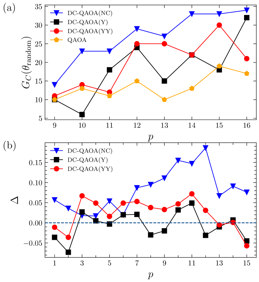
In Fig. 5(b) we show the comparison of the suppression ability as functions of for the three types of DC-QAOA with 15 layers trained on a graph with 16 vertices. A positive indicates that the cd-terms are effective in increasing the approximate ratio, and in turn, the efficiency of the algorithm. We see that for the case of DC-QAOA(NC), is positive for the entire range of , while for other methods fluctuates between positive and negative values. If we focus on the range , DC-QAOA(NC) has values higher than any other methods. This fact indicates the strong ability of DC-QAOA(NC) to suppress unwanted excitation and to add the effective dimensions, and thus its superior performance. On the other hand, the suppression ability for DC-QAOA(Y) and DC-QAOA(YY) are only positive for intermediate values, limiting its efficiency. This also explains why DC-QAOA(Y) and DC-QAOA(YY) do not exhibit considerable advantage over QAOA-3.
III.3 Instance-Sequential Training (IST)
In previous sections, we have shown that DC-QAOA can be more advantageous than QAOA under certain conditions, because the former has accelerated critical depth scaling behavior and more effective dimensions to suppress non-diagonal transitions. In this section, we study the distribution of optimal parameters resulting from a judiciously trained DC-QAOA(NC). We shall show that these parameters are more concentrated in the parameter space, and based on this fact, we propose an IST method, which can substantially improve the efficiency in training.
For a -layer QAOA defined on qubits, the optimal parameters are said to be concentrated if:
| (13) |
where may not be the unique optimal parameters, can guarantee that the optimal parameters will converge to a limit when Akshay et al. (2021), and is the distance between optimal parameters found for two graphs whose number of vertices differ by one. For DC-QAOA(NC), parameter concentration can be similarly defined on .
The dimension of the parameter space is typically high, and to visualize it we use the t-SNE algorithm van der Maaten and Hinton (2008). This algorithm is ubiquitously used for dimensionality reduction while maintaining the local structure of the data, making clusters in the original high-dimensional space more apparent and easily identifiable in the reduced-dimensional space van der Maaten and Hinton (2008).
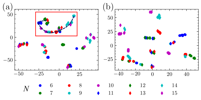
We focus on the set of graphs as shown in Fig. 9. For each graph, we optimize 10 sets of parameters of DC-QAOA(NC) and QAOA respectively from random initial parameters, in a 10-layer DC-QAOA(NC) and QAOA respectively. In Fig. 6, all optimal parameters are embedded into two dimensions to visualize by t-SNE algorithm. For DC-QAOA(NC) in Fig. 6(a), at least one set of optimal parameter of all graph size appears within the red box and roughly forms a curly shaped trajectory, whereas for QAOA in Fig. 6(b), optimal parameters are more scattered, only creating small-scale clusters, if any, in different regions.
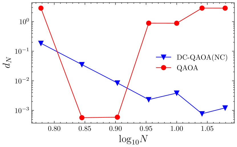
To examine parameter concentration in a more quantitative fashion, the distance between and for QAOA and the distance between and for DC-QAOA(NC) are plotted against the logarithm of number of qubits in Fig. 7. Distance is calculated between two closest ones from 100 sets of optimal parameters between graphs with qubits and qubits. For DC-QAOA(NC), the logarithm of the distance shows a linear trend with number of qubits, indicating that there is a consistent trend of parameter concentration in DC-QAOA(NC) with , implying that optimal parameters of DC-QAOA will converge to a limit when is large enough.
To fully leverage the advantage afforded by such phenomenon of parameter concentration in DC-QAOA(NC), we propose the IST method, that can make the training process of DC-QAOA(NC) more efficient in using quantum resources. Under the IST method, for a graph with vertices, we randomly remove vertices (and the edges associated with them) while keeping the graph connected, i.e. the graph should not be separated to two. Firstly, we train DC-QAOA(NC) on the remaining vertices to get optimal parameters . Then, one vertex is added back to the graph (and the edges associated with it) and DC-QAOA(NC) is trained again using as the starting point to obtain . We then add one more vertex back, and the above steps are repeated until is obtained.
On the other hand, traditional training method needs to construct a circuit on qubits based on the connected edges in the graph. The number of CNOT gates in and are the same as the number of edges in the graph, which, for large problems necessarily complicating the circuit, makes it more prone to decoherence. In order to quantify and compare the quantum resources used in the two training methods, we use the product of number of qubits , number of CNOT gates (equivalent to for DC-QAOA(NC) and for QAOA respectively, where is the number of edges in the graph ) and number of training iterations as an indicator. The proposed indicator for comparing quantum resources captures three critical dimensions of resource usage in quantum training:
-
•
Number of qubits represents the system size, directly influencing the computational complexity and the memory resources required to simulate or run the quantum system.
-
•
Number of CNOT gates () reflects the entangling operations, which are among the most resource-intensive quantum operations due to their role in creating quantum correlations.
-
•
Training iterations represent the temporal aspect of resource consumption, as more iterations correspond to greater computation time.
Together, this indicator effectively quantifies the overall computational burden by incorporating both spatial (qubits and CNOT gates) and temporal (iterations) aspects, giving a holistic view of the quantum resources consumed during the training process. The quantum resources used in the two training methods are summarized in Table 2. It is clear that , which means that IST uses at most half of quantum resources used by traditional method when is sufficiently small compared to as in the case of large-scale quantum optimization where is large.
| Method | Quantum Resources |
|---|---|
| IST | |
| Traditional |
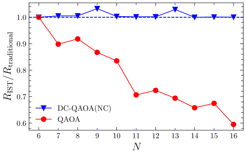
To demonstrate the effectiveness of the IST method, we compare it to the traditional training method while fixing the number of total training iterations the same. In this comparison, the IST method uses much fewer quantum resources because it does not have to access all qubits in the quantum processing unit in every iteration. We benchmark the advantage of performance by the proportion of approximate ratio of the IST method relative to the one for traditional method . In Fig. 8, the performance of DC-QAOA(NC) trained using IST method is nearly the same with the one trained using traditional method using much less quantum resources. Sometimes, for and 13 DC-QAOA(NC) trained using IST works even better than the one trained using traditional method. However, for QAOA, the IST method fails due to the lack of parameter concentration. We conclude that when the number of training iterations are held same for both methods, IST method, on average, takes less time to run a quantum devices and use fewer qubits to construct the circuits. This is a favorable characteristic especially when the access to the device is limited by certain quota, e.g. cloud-based ones.
IV CONCLUSION
In this work, we have used the MaxCut problem as an example to throughly examine the comparison between DC-QAOA and QAOA. Such a comparison has been previously done with the number of layers held equal and with a conclusion that DC-QAOA is superior to QAOA for all sizes of the problem. However, we demonstrate that this statement must be carefully refined according to the actual circuit complexity afforded by different algorithms, which includes both the number of layers and number of CNOT gates in each layer. The cd-terms introduced in DC-QAOA reduces the critical depth of the algorithm but also introduces additional CNOT gates, so the overall circuit complexity is not necessarily lower than QAOA without cd-terms. We have found that for MaxCut problem with , QAOA is more advantageous than DC-QAOA(NC), while for larger problems with , DC-QAOA(NC) is superior. This refinement of the comparison between the two algorithms has not been previously noted in the literature. Although both YY and Y types of cd-terms enhance the performance of QAOA, the magnitude of improvement is not as significant as that achieved by DC-QAOA(NC).
Furthermore, we calculated the effective dimensions of the algorithms and have shown that the superior performance of DC-QAOA(NC) in larger problems is rooted in its strong ability to suppress unwanted excitation and to add the effective dimensions. We have also noted that the optimal parameters found by DC-QAOA(NC) is more concentrated than those from QAOA. Based on this finding, we introduced an IST training method, which achieves similar (and sometimes even better) results as compared to traditional trining methods, while consuming much fewer quantum resources. Our results should be valuable to recent efforts in utilizing VQA to solve combinatorial optimization problems for large-scale computational tasks, thereby advancing the study of quantum optimization.
ACKNOWLEDGEMENT
This work is supported by the National Natural Science Foundation of China (Grant No. 11874312, 12474489), the Research Grants Council of Hong Kong (CityU 11304920), the Guangdong Provincial Quantum Science Strategic Initiative (Grant No. GDZX2203001, GDZX2303007), and the Innovation Program for Quantum Science and Technology (Grant No. 2021ZD0302300).
APPENDIX
For completeness, in Fig. 9 we show all graphs used in the study. These graphs are randomly generated, subject to the condition that the edges between every pair of vertices are connected with probability with networkxHagberg et al. (2008).
References
- Cerezo et al. (2021) M. Cerezo, A. Arrasmith, R. Babbush, S. C. Benjamin, S. Endo, K. Fujii, J. R. McClean, K. Mitarai, X. Yuan, L. Cincio, and P. J. Coles, Nat. Rev. Phys. 3, 625 (2021).
- Kandala et al. (2017) A. Kandala, A. Mezzacapo, K. Temme, M. Takita, M. Brink, J. M. Chow, and J. M. Gambetta, Nature 549, 242 (2017).
- Mitarai et al. (2018) K. Mitarai, M. Negoro, M. Kitagawa, and K. Fujii, Phys. Rev. A 98, 032309 (2018).
- McClean et al. (2016) J. R. McClean, J. Romero, R. Babbush, and A. Aspuru-Guzik, New J. Phys. 18, 023023 (2016).
- Liu et al. (2019) J.-G. Liu, Y.-H. Zhang, Y. Wan, and L. Wang, Phys. Rev. Res. 1, 023025 (2019).
- Peruzzo et al. (2014) A. Peruzzo, J. McClean, P. Shadbolt, M.-H. Yung, X.-Q. Zhou, P. J. Love, A. Aspuru-Guzik, and J. L. O’Brien, Nat. Commun. 5, 4213 (2014).
- Haug et al. (2021) T. Haug, K. Bharti, and M. S. Kim, PRX Quantum 2, 040309 (2021).
- Abbas et al. (2021) A. Abbas, D. Sutter, C. Zoufal, A. Lucchi, A. Figalli, and S. Woerner, Nat. Comput. Sci. 1, 403 (2021).
- Comparat (2009) D. Comparat, Phys. Rev. A 80, 012106 (2009).
- Hadfield et al. (2019) S. Hadfield, Z. Wang, B. O’Gorman, E. Rieffel, D. Venturelli, and R. Biswas, Algorithms 12, 34 (2019).
- Zhou et al. (2020) L. Zhou, S.-T. Wang, S. Choi, H. Pichler, and M. D. Lukin, Phys. Rev. X 10, 021067 (2020).
- Zhou et al. (2023) Z. Zhou, Y. Du, X. Tian, and D. Tao, Phys. Rev. Appl. 19, 024027 (2023).
- Zhu et al. (2022) L. Zhu, H. L. Tang, G. S. Barron, F. A. Calderon-Vargas, N. J. Mayhall, E. Barnes, and S. E. Economou, Phys. Rev. Res. 4, 033029 (2022).
- Ruan et al. (2023) Y. Ruan, Z. Yuan, X. Xue, and Z. Liu, Inf. Sci. 619, 98 (2023).
- Oh et al. (2019) Y.-H. Oh, H. Mohammadbagherpoor, P. Dreher, A. Singh, X. Yu, and A. J. Rindos, “Solving multi-coloring combinatorial optimization problems using hybrid quantum algorithms,” (2019), arxiv:1911.00595 .
- Farhi et al. (2014) E. Farhi, J. Goldstone, and S. Gutmann, “A quantum approximate optimization algorithm,” (2014), arxiv:1411.4028 .
- Chen et al. (2010) X. Chen, A. Ruschhaupt, S. Schmidt, A. del Campo, D. Guéry-Odelin, and J. G. Muga, Phys. Rev. Lett. 104, 063002 (2010).
- Vacanti et al. (2014) G. Vacanti, R. Fazio, S. Montangero, G. M. Palma, M. Paternostro, and V. Vedral, New J. Phys. 16, 053017 (2014).
- Ji et al. (2022) Y. Ji, F. Zhou, X. Chen, R. Liu, Z. Li, H. Zhou, and X. Peng, Phys. Rev. A 105, 052422 (2022).
- Hartmann and Lechner (2019) A. Hartmann and W. Lechner, New J. Phys. 21, 043025 (2019).
- Hegade et al. (2021) N. N. Hegade, K. Paul, Y. Ding, M. Sanz, F. Albarrán-Arriagada, E. Solano, and X. Chen, Phys. Rev. Appl. 15, 024038 (2021).
- Chandarana et al. (2022) P. Chandarana, N. N. Hegade, K. Paul, F. Albarrán-Arriagada, E. Solano, A. Del Campo, and X. Chen, Phys. Rev. Res. 4, 013141 (2022).
- Ding et al. (2024) Q.-M. Ding, Y.-M. Huang, and X. Yuan, Phys. Rev. Appl. 21, 034036 (2024).
- Chandarana et al. (2023) P. Chandarana, N. N. Hegade, I. Montalban, E. Solano, and X. Chen, Phys. Rev. Appl. 20, 014024 (2023).
- Hegade et al. (2022) N. N. Hegade, P. Chandarana, K. Paul, X. Chen, F. Albarrán-Arriagada, and E. Solano, Phys. Rev. Res. 4, 043204 (2022).
- Aoshima and Iri (1977) K. Aoshima and M. Iri, SIAM J. Comput. 6, 86 (1977).
- Barends et al. (2016) R. Barends, A. Shabani, L. Lamata, J. Kelly, A. Mezzacapo, U. L. Heras, R. Babbush, A. G. Fowler, B. Campbell, Y. Chen, Z. Chen, B. Chiaro, A. Dunsworth, E. Jeffrey, E. Lucero, A. Megrant, J. Y. Mutus, M. Neeley, C. Neill, P. J. J. O’Malley, C. Quintana, P. Roushan, D. Sank, A. Vainsencher, J. Wenner, T. C. White, E. Solano, H. Neven, and J. M. Martinis, Nature 534, 222 (2016).
- Sels and Polkovnikov (2017) D. Sels and A. Polkovnikov, Proc. Natl. Acad. Sci. U.S.A. 114, E3909 (2017).
- Čepaitė et al. (2023) I. Čepaitė, A. Polkovnikov, A. J. Daley, and C. W. Duncan, PRX Quantum 4, 010312 (2023).
- Chai et al. (2022) Y. Chai, Y.-J. Han, Y.-C. Wu, Y. Li, M. Dou, and G.-P. Guo, Phys. Rev. A 105, 042415 (2022).
- Goemans and Williamson (1995) M. X. Goemans and D. P. Williamson, J. ACM 42, 1115 (1995).
- Akshay et al. (2022) V. Akshay, H. Philathong, E. Campos, D. Rabinovich, I. Zacharov, X.-M. Zhang, and J. D. Biamonte, Phys. Rev. A 106, 042438 (2022).
- Akshay et al. (2021) V. Akshay, D. Rabinovich, E. Campos, and J. Biamonte, Phys. Rev. A 104, L010401 (2021).
- van der Maaten and Hinton (2008) L. van der Maaten and G. Hinton, J. Mach. Learn. Res. 9, 2579 (2008).
- Hagberg et al. (2008) A. Hagberg, P. Swart, and D. S Chult, Exploring network structure, dynamics, and function using NetworkX, Tech. Rep. (Los Alamos National Lab.(LANL), Los Alamos, NM (United States), 2008).