Cucheb: a GPU implementation of the filtered Lanczos procedure111This work was partially supported by the European Research Council under the European Union’s Seventh Framework Programme (FP7/2007–2013)/ERC grant agreement no. 291068. The views expressed in this article are not those of the ERC or the European Commission, and the European Union is not liable for any use that may be made of the information contained here; and by the Scientific Discovery through Advanced Computing (SciDAC) program funded by U.S. Department of Energy, Office of Science, Advanced Scientific Computing Research and Basic Energy Sciences DE-SC0008877.
Abstract
This paper describes the software package Cucheb, a GPU implementation of the filtered Lanczos procedure for the solution of large sparse symmetric eigenvalue problems. The filtered Lanczos procedure uses a carefully chosen polynomial spectral transformation to accelerate convergence of the Lanczos method when computing eigenvalues within a desired interval. This method has proven particularly effective for eigenvalue problems that arise in electronic structure calculations and density functional theory. We compare our implementation against an equivalent CPU implementation and show that using the GPU can reduce the computation time by more than a factor of 10.
keywords:
GPU, eigenvalues, eigenvectors, quantum mechanics, electronic structure calculations, density functional theoryProgram title: Cucheb
Licensing provisions: MIT
Programming language: CUDA C/C++
Nature of problem: Electronic structure calculations require the
computation of all eigenvalue-eigenvector pairs of a symmetric matrix that lie
inside a user-defined real interval.
Solution method: To compute all the eigenvalues within a given interval a
polynomial spectral transformation is constructed that maps the desired
eigenvalues of the original matrix to the exterior of the spectrum of the
transformed matrix. The Lanczos method is then used to compute the desired
eigenvectors of the transformed matrix, which are then used to recover the
desired eigenvalues of the original matrix. The bulk of the operations are
executed in parallel using a graphics processing unit (GPU).
Runtime: Variable, depending on the number of eigenvalues sought and
the size and sparsity of the matrix.
1 Introduction
This paper describes the software package Cucheb, a GPU implementation of the filtered Lanczos procedure [1]. The filtered Lanczos procedure (FLP) uses carefully chosen polynomial spectral transformations to accelerate the computation of all the eigenvalues and corresponding eigenvectors of a real symmetric matrix inside a given interval. The chosen polynomial maps the eigenvalues of interest to the extreme part of the spectrum of the transformed matrix. The Lanczos method [2] is then applied to the transformed matrix which typically converges quickly to the invariant subspace corresponding to the extreme part of the spectrum. This technique has been particularly effective for large sparse eigenvalue problems arising in electronic structure calculations [3, 4, 5, 6, 7].
In the density functional theory framework (DFT) the solution of the all-electron Schrödinger equation is replaced by a one-electron Schrödinger equation with an effective potential which leads to a nonlinear eigenvalue problem known as the Kohn-Sham equation [8, 9]:
| (1) |
where is a wave function and is a Kohn-Sham eigenvalue. The ionic potential reflects contributions from the core and depends on the position only. Both the Hartree and the exchange-correlation potentials depend on the charge density:
| (2) |
where is the number of occupied states (for most systems of interest this is half the number of valence electrons). Since the total potential depends on which itself depends on eigenfunctions of the Hamiltonian, Equation (1) can be viewed as a nonlinear eigenvalue problem or a nonlinear eigenvector problem. The Hartree potential is obtained from by solving the Poisson equation with appropriate boundary conditions. The exchange-correlation term is the key to the DFT approach and it captures the effects of reducing the problem from many particles to a one-electron problem, i.e., from replacing wavefunctions with many coordinates into ones that depend solely on space location .
Self-consistent iterations for solving the Kohn-Sham equation start with an initial guess of the charge density , from which a guess for is computed. Then (1) is solved for ’s and a new is obtained from (2) and the potentials are updated. Then (1) is solved again for a new obtained from the new ’s, and the process is repeated until the total potential has converged.
A typical electronic structure calculation with many atoms requires the calculation of a large number of eigenvalues, specifically the leftmost ones. In addition, calculations based on time-dependent density functional theory [10, 11], require a substantial number of unoccupied states, states beyond the Fermi level, in addition to the occupied ones. Thus, it is not uncommon to see eigenvalue problems in the size of millions where tens of thousands of eigenvalues may be needed.
Efficient numerical methods that can be easily parallelized in current high-performance computing environments are therefore essential in electronic structure calculations. The high computational power offered by GPUs has increased their presence in the numerical linear algebra community and they are gradually becoming an important tool of scientific codes for solving large-scale, computationally intensive eigenvalue problems. While GPUs are mostly known for their high speedups relative to CPU-bound operations222See also the MAGMA project at http://icl.cs.utk.edu/magma/index.html, sparse eigenvalue computations can also benefit from hybrid CPU-GPU architectures. Although published literature and scientific codes for the solution of sparse eigenvalue problems on a GPU have not been as common as those that exist for multi-CPU environments, recent studies conducted independently by some of the authors of this paper demonstrated that the combination of polynomial filtering eigenvalue solvers with GPUs can be beneficial [12, 13].
The goal of this paper is twofold. First we describe our open source software package Cucheb333https://github.com/jaurentz/cucheb that uses the filtered Lanczos procedure to accelerate large sparse eigenvalue computations using Nvidia brand GPUs. Then we demonstrate the effectiveness of using GPUs to accelerate the filtered Lanczos procedure by solving a set of eigenvalue problems originating from electronic stucture calculations with Cucheb and comparing it with a similar CPU implementation.
The paper is organized as follows. Section 2 introduces the concept of polynomial filtering for symmetric eigenvalue problems and provides the basic formulation of the filters used. Section 3 discusses the proposed GPU implementation of the filtered Lanczos procedure. Section 4 presents computational results with the proposed GPU implementations. Finally, concluding remarks are presented in Section 5.
2 The filtered Lanczos procedure
The Lanczos algorithm and its variants [2, 14, 15, 16, 17, 18, 19] are well-established methods for computing a subset of the spectrum of a real symmetric matrix. These methods are especially adept at approximating eigenvalues lying at the extreme part of the spectrum [20, 21, 22, 23]. When the desired eigenvalues are well inside the spectral interval these techniques can become ineffective and lead to large computational and memory costs. Traditionally, this is overcome by mapping interior eigenvalues to the exterior part using a shift-and-invert spectral transformation (see for example [24] or [25]). While shift-and-invert techniques typically work very well, they require solving linear systems involving large sparse matrices which can be difficult or even infeasible for certain classes of matrices.
The filtered Lanczos procedure (FLP) offers an appealing alternative for such cases. In this approach interior eigenvalues are mapped to the exterior of the spectrum using a polynomial spectral transformation. Just as with shift-and-invert, the Lanczos method is then applied to the transformed matrix [1]. The key difference is that polynomial spectral transformations only require matrix-vector multiplication, a task that is often easy to parallelize for sparse matrices. For FLP constructing a good polynomial spectral transformation is the most important prepocessing step.
2.1 Polynomial spectral transformations
Let be symmetric and let
| (3) |
be its spectral decomposition, where is an orthogonal matrix and is real and diagonal. A spectral transformation of is a mapping of the form
| (4) |
where and is any (real or complex) function defined on the spectrum of . Standard examples in eigenvalue computations include the shift-and-invert transformation and for subspace iteration.
A polynomial spectral transformation or filter polynomial is any spectral transformation that is also a polynomial. For the filtered Lanczos procedure a well constructed filter polynomial means rapid convergence and a good filter polynomial should satisfy the following requirements: a) the desired eigenvalues of are the largest in magnitude eigenvalues of , b) the construction of requires minimal knowledge of the spectrum of , and c) multiplying a vector by is relatively inexpensive and easy to parallelize.
Our implementation of the FLP constructs polynomials that satisfy the above requirements using techniques from digital filter design. The basic idea is to construct a polynomial filter by approximating an “ideal” filter which maps the desired eigenvalues of to eigenvalues of largest magnitude in .
2.2 Constructing polynomial transformations
Throughout this section it is assumed that the spectrum of is contained entirely in the interval . In practice, this assumption poses no restrictions since the eigenvalues of located inside the interval , where denote the algebraically smallest and largest eigenvalues of respectively, can be mapped to the interval by the following linear transformation:
| (5) |
Since and are exterior eigenvalues of , one can obtain very good estimates by performing a few Lanczos steps. We will see in Section 4 that computing such estimates constitutes only a modest fraction of the total compute time.
Given a subinterval we wish to compute all eigenvalues of in along with their corresponding eigenvectors. Consider first the following spectral transformation:
| (6) |
The function is just an indicator function, taking the value 1 inside the interval and zero outside. When acting on , maps the desired eigenvalues of to the repeated eigenvalue for and all the unwanted eigenvalues to . Moreover, the invariant subspace which corresponds to eigenvalues of within the interval is identical to the invariant subspace of which corresponds to the multiple eigenvalue 1. Thus, applying Lanczos on computes the same invariant subspace, with the key difference being that the eigenvalues of interest (mapped to one) are well-separated from the unwanted ones (mapped to zero), and rapid convergence can be established. Unfortunately, such a transformation is not practically significant as there is no cost-effective way to multiply a vector by .
A practical alternative is to replace with a polynomial such that for all . Such a will then map the desired eigenvalues of to a neighborhood of for . Moreover, since is a polynomial, applying to a vector only requires matrix-vector multiplication with .
In order to quickly construct a that is a good approximation to it is important that we choose a good basis. For functions supported on the obvious choice is Chebyshev polynomials of the first kind. Such representations have already been used successfully for constructing polynomial spectral transformations and for approximating matrix-valued functions in quantum mechanics (see for example [13, 26, 1, 27, 28, 4, 5, 3, 29, 30, 6]).
Recall that the Chebyshev polynomials of the first kind obey the following three-term recurrence
| (7) |
starting with , . The Chebyshev polynomials also satisfy the following orthogonality condition and form a complete orthogonal set for the Hilbert space , :
| (8) |
Since it possesses a convergent Chebyshev series
| (9) |
where the are defined as follows:
| (10) |
where represents the Dirac delta symbol. For a given and the are known analytically (see for example [31]),
| (11) |
An obvious choice for constructing is to fix a degree and truncate the Chebyshev series of ,
| (12) |
Due to the discontinuities of , does not converge to uniformly as . The lack of uniform convergence is not an issue as long as the filter polynomial separates the wanted and unwanted eigenvalues. Figure 1 illustrates two polynomial spectral transformations constructed by approximating on two different intervals. Even with the rapid oscillations near the ends of the subinterval, these polynomials are still good candidates for separating the spectrum.
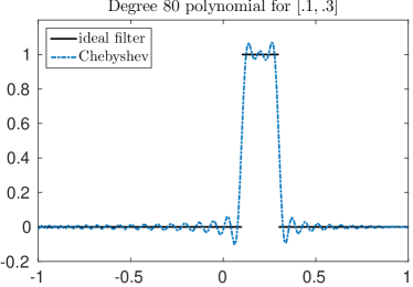
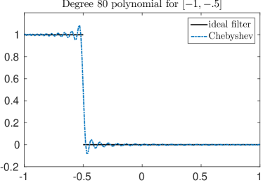
Figure 1 shows approximations of the ideal filter for two different subintervals of , using a fixed degree . In the left subfigure the interval of interest is located around the middle of the spectrum , while in the right subfigure the interval of interest is located at the left extreme part . Note that the oscillations near the discontinuities do not prevent the polynomials from separating the spectrum.
Since is sparse, multiplying by a vector can be done efficiently in parallel using a vectorized version of Clenshaw’s algorithm [32] when is represented in a Chebyshev basis. Moreover Clenshaw’s algorithm can be run entirely in real arithmetic whenever the Chebyshev coefficients of are real.
2.3 Filtered Lanczos as an algorithm
Assuming we’ve constructed a polynomial filter , we can approximate eigenvalues of by first approximating eigenvalues and eigenvectors of using a simple version of the Lanczos method [2]. Many of the matrices arising in practical applications possess repeated eigenvalues, requiring the use of block Lanczos algorithm [17], so we describe the block version of FLP as it contains the standard algorithm as a special case.
Given a block size and a matrix with orthonormal columns, the filtered Lanzos procedure iteratively constructs an orthonormal basis for the Krylov subspace generated by and :
| (13) |
Let us denote by the matrix whose columns are generated by steps of the block Lanczos algorithm. Then, for each integer we have and . Since is symmetric the columns of can be generated using short recurrences. This implies that there exists symmetric and upper-triangular , , such that
| (14) |
where
| (15) |
and denotes the last columns of the identity matrix of size . Left multiplying (14) by gives the Rayleigh-Ritz projection
| (16) |
The matrix is symmetric and banded, with a semi-bandwidth of size . The eigenvalues of are the Ritz values of associated with the subspace spanned by the columns of and for sufficiently large the dominant eigenvalues of will be well approximated by these Ritz values. Of course we aren’t actually interested in the eigenvalues of but those of . We can recover these eigenvalues by using the fact that has the same eigenvectors as . Assuming that an eigenvector of has been computed accurately we can recover the corresponding eigenvalue of from the Rayleigh quotient of :
| (17) |
In practice we will often have only a good approximation of . The approximate eigenvector will be a Ritz vector of associated with . To compute these Ritz vectors we first compute an eigendecomposition of . Since is real and symmetric there exists an orthogonal matrix and a diagonal matrix such that
| (18) |
Combining (14) and (18), the Ritz vectors of are formed as .
3 Cucheb: a GPU implementation of the filtered Lanczos procedure
A key advantage of the filtered Lanczos procedure is that it requires only matrix-vector multiplication, an operation that uses relatively low memory and that is typically easy to parallelize compared to solving large linear systems. FLP and related methods have already been successfully implemented on multi-core CPUs and distributed memory machines [3].
3.1 The GPU architecture
A graphical processing unit (GPU) is a single instruction multiple data (SIMD) scalable model which consists of multi-threaded streaming Multiprocessors (SMs), each one equipped with multiple scalar processor cores (SPs), with each SP performing the same instruction on its local portion of data. While they were initially developed for the purposes of graphics processing, GPUs were adapted in recent years for general purpose computing. The development of the Compute Unified Device Architecture (CUDA) [33] parallel programming model by Nvidia, an extension of the C language, provides an easy way for computational scientists to take advantage of the GPU’s raw power.
Although the CUDA programming language allows low level access to Nvidia GPUs, the Cucheb library accesses the GPU through high level routines included as part of the Nvidia CUDA Toolkit. The main advantage of this is that one only has to update to the latest version of the Nvidia’s toolkit in order to make use of the latest GPU technology.
3.2 Implementation details of the Cucheb software package
In this section we discuss the details of our GPU implementation of FLP. Our implementation will consist of a high-level, open source C++ library called Cucheb [34] which depends only on the Nvidia CUDA Toolkit [35, 33] and standard C++ libraries, allowing for easy interface with Nvidia brand GPUs. At the user level, the Cucheb software library consists of three basic data structures:
-
1.
cuchebmatrix
-
2.
cucheblanczos
-
3.
cuchebpoly
The remainder of this section is devoted to describing the role of each of these data structures.
3.2.1 Sparse matrices and the cuchebmatrix object
The first data structure, called cuchebmatrix, is a container for storing and manipulating sparse matrices. This data structure consists of two sets of pointers, one for data stored in CPU memory and one for data stored in GPU memory. Such a duality of data is often necessary for GPU computations if one wishes to avoid costly memory transfers between the CPU and GPU. To initialize a cuchebmatrix object one simply passes the path to a symmetric matrix stored in the matrix market file format [36]. The following segment of Cucheb code illustrates how to initialize a cuchebmatrix object using the matrix H2O downloaded from the University of Florida sparse matrix collection [37]:
#include "cucheb.h"

int main(){

  // declare cuchebmatrix variable
  cuchebmatrix ccm;

  // create string with matrix market file name
  string mtxfile("H2O.mtx");

  // initialize ccm using matrix market file
  cuchebmatrix_init(&mtxfile, &ccm);

  .
  .
  .

}
The function cuchebmatrix_init opens the data file, checks that the
matrix is real and symmetric, allocates the required memory on the CPU and GPU,
reads the data into CPU memory, converts it to an appropriate format for the
GPU and finally copies the data into GPU memory. By appropriate format we mean
that the matrix is stored on the GPU in compressed sparse row (CSR) format with
no attempt to exploit the symmetry of the matrix. CSR is used as it is one of
the most generic storage scheme for performing sparse matrix-vector
multiplications using the GPU. (See [38, 39] and references
therein for a discussion on the performance of sparse matrix-vector
multiplications in the CSR and other formats.) Once a cuchebmatrix object has been
created, sparse matrix-vector multiplications can then be performed on the GPU
using the Nvidia CUSPARSE library [40].
3.2.2 Lanczos and the cucheblanczos object
The second data structure, called cucheblanczos, is a container for storing and
manipulating the vectors and matrices associated with the Lanczos process. As
with the cuchebmatrix objects, a cucheblanczos object possesses pointers to both CPU and GPU
memory. While there is a function for initializing a cucheblanczos object, the average
user should never do this explicitly. Instead they should call a higher level
routine like
cuchebmatrix_lanczos which takes as an argument an
uninitialized cucheblanczos object. Such a routine will then calculate an appropriate
number of Lanczos vectors based on the input matrix and initialize the cucheblanczos object accordingly.
Once a cuchebmatrix object and corresponding cucheblanczos object have been initialized, one of the core Lanczos algorithms can be called to iteratively construct the Lanczos vectors. Whether iterating with or , the core Lanczos routines in Cucheb are essentially the same. The algorithm starts by constructing an orthonormal set of starting vectors (matrix in (13)). Once the vectors are initialized the algorithm expands the Krylov subspace, peridiocally checking for convergence. To check convergence the projected problem (18) is copied to the CPU, the Ritz values are computed and the residuals are checked. If the algorithm has not converged the Krylov subspace is expanded further and the projected problem is solved again. For stability reasons Cucheb uses full reorthogonalization to expand the Krylov subspace, making the algorithm more akin to the Arnoldi method [41]. Due to the full reorthogonalization, the projected matrix from (18) will not be symmetric exactly but it will be symmetric to machine precision, which justifies the use of an efficient symmetric eigensolver (see for example [42]). The cost of solving the projected problem is negligible compared to expanding the Krylov subspace, so we can afford to check convergence often. All the operations required for reorthogonalization are performed on the GPU using the Nvidia CUBLAS library [43]. Solving the eigenvalue problem for is done on the CPU using a special purpose built banded symmetric eigensolver included in the Cucheb library.
It is possible to use selective reorthogonalization [44, 23, 45] or implicit restarts [14, 15], though we don’t make use of these techniques in our code. In Section 4 we will see that the dominant cost in the algorithm is the matrix-vector multiplication with , so reducing the number of products with is the easiest way to shorten the computation time. Techniques like implicit restarting can often increase the number of iterations if the size of the maximum allowed Krylov subspace is too small, meaning we would have to perform more matrix-vector multiplications. Our experience suggests that the best option is to construct a good filter polynomial and then compute increasingly larger Krylov subspaces until the convergence criterion is met.
All the Lanczos routines in Cucheb are designed to compute all the eigenvalues in a user prescribed interval . When checking for convergence the Ritz values and vectors are sorted according to their proximity to and the method is considered to be converged when all the Ritz values in as well as a few of the nearest Ritz values outside the interval have sufficiently small residuals. If the iterations were done using then the computation is complete and the information is copied back to the CPU. If the iterations were done with the Rayleigh quotients are first computed on the GPU and then the information is copied back to the CPU.
To use Lanczos with to compute all the eigenvalues in a user is required to input five variables:
-
1.
a lower bound on the desired spectrum ()
-
2.
an upper bound on the desired spectrum ()
-
3.
a block size
-
4.
an initialized cuchebmatrix object
-
5.
an uninitialized cucheblanczos object
The following segment of Cucheb code illustrates how to do this using the
function cuchebmatrix_lanczos for the interval , a block
size of and an already initialized cuchebmatrix object:
#include "cucheb.h"

int main(){

  // initialize cuchebmatrix object
  cuchebmatrix ccm;
  string mtxfile("H2O.mtx");
  cuchebmatrix_init(&mtxfile, &ccm);

  // declare cucheblanczos variable
  cucheblanczos ccl;

  // compute eigenvalues in [.5,.6] using block Lanczos
  cuchebmatrix_lanczos(.5, .6, 3, &ccm, &ccl);

  .
  .
  .

}
This function call will first approximate the upper and lower bounds on the
spectrum of the cuchebmatrix object. It then uses these bounds to make sure that the
interval is valid. If it is, it will adaptively build up the Krylov
subspace as described above, periodically checking for convergence. For large
matrices or subintervals well inside the spectrum, standard Lanczos may fail to
converge all together. A better choice is to call the routine
cuchebmatrix_filteredlanczos which automatically constructs a filter
polynomial and then uses FLP to compute all the eigenvalues in .
3.2.3 Filter polynomials and the cuchebpoly object
To use FLP one needs a way to store and manipulate filter polynomials stored in a Chebyshev basis. In Cucheb this is done with the cuchebpoly object. The cuchebpoly object contains pointers to CPU and GPU memory which can be used to construct and store filter polynomials. For the filter polynomials from Section 2 one only needs to store the degree, the Chebyshev coefficients and upper and lower bounds for the spectrum of .
As with cucheblanczos objects, a user typically will not need to initialize a cuchebpoly object themselves as it will be handled automatically by a higher level
routine. In cuchebmatrix_filteredlanczos for example, not only is the
cuchebpoly object for the filter polynomial initialized but also the degree at which
the Chebyshev approximation should be truncated is computed. This is done using
a simple formula based on heuristics and verified by experiment. Assuming the
spectrum of is in , a “good” degree for
is computed using the following formula:
| (19) |
where is the weighted Chebyshev -norm. The tolerance is a parameter and is chosen experimentally, with the goal of maximizing the separation power of the filter while keeping the polynomial degree and consequently the computation time low.
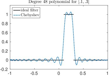
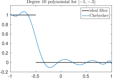
Figure 2 uses the same ideal filters from Figure 1 but this time computes the filter degree based on (19). In the left subfigure the interval of interest is located around the middle of the spectrum and the distance between and is relatively small, giving a filter degree of . In the right subfigure the interval of interest is located at the left extreme part of the spectrum and the distance and is relatively large, giving a filter degree of . Although these filters seem like worse approximations than those in Figure 1, the lower degrees lead to much shorter computation times.
The following segment of Cucheb code illustrates how to use the function
cuchebmatrix_filteredlanczos to compute all the eigenvalues in the
interval of an already initialized cuchebmatrix object using FLP with
a block size of :
#include "cucheb.h"

int main(){

  // initialize cuchebmatrix object
  cuchebmatrix ccm;
  string mtxfile("H2O.mtx");
  cuchebmatrix_init(&mtxfile, &ccm);

  // declare cucheblanczos variable
  cucheblanczos ccl;

  // compute eigenvalues in [.5,.6] using filtered Lanczos
  cuchebmatrix_filteredlanczos(.5, .6, 3, &ccm, &ccl);

  .
  .
  .

}
4 Experiments
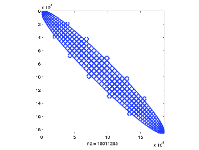
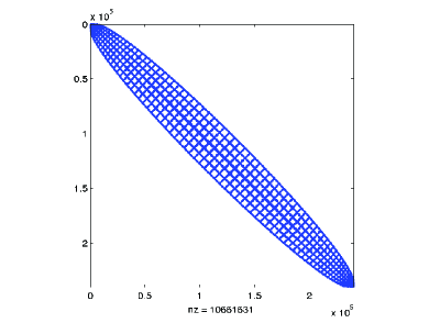
In this section we illustrate the performance of our GPU implementation of the filtered Lanczos procedure. Our test matrices (Hamiltonians) originate from electronic structure calculations. In this setting, one is typically interested in computing a few eigenvalues around the Fermi level of each Hamiltonian. The Hamiltonians were generated using the PARSEC package [46] and can be also found in the University of Florida sparse matrix collection [37].444https://www.cise.ufl.edu/research/sparse/matrices/ These Hamiltonians are real, symmetric, and have clustered, as well as multiple, eigenvalues. Table 1 lists the size , the total number of non-zero entries , as well as the endpoints of the spectrum of each matrix, i.e., the interval defined by the algebraically smallest/largest eigenvalues. The average number of nonzero entries per row for each Hamiltonian is quite large, a consequence of the high-order discretization and the addition of a (dense) ‘non-local’ term. Figure 3 plots the sparsity pattern of matrices Si41Ge41H72 (left) and Si87H76 (right).
All GPU experiments in this section were implemented using the Cucheb library and performed on the same machine which has an Intel Xeon E5-2680 v3 2.50GHz processor with 128GB of CPU RAM and two Nvidia K40 GPUs each with 12GB of GPU RAM and 2880 compute cores. We make no attempt to access mutliple GPUs and all the experiments were performed using a single K40.
| Matrix | Spectral interval | |||
|---|---|---|---|---|
Ge87H76 |
||||
Ge99H100 |
||||
Si41Ge41H72 |
||||
Si87H76 |
||||
Ga41As41H72 |
Exploiting eigenvalue solvers that are based on matrix factorizations, e.g., shift-and-invert techniques, has been shown to be impractical for matrices of the PARSEC matrix collection [47, 48]. The reason is that performing the LU factorization of each Hamiltonian results in a huge amount of fill-in in the associated triangular factors, requiring an excessive amount of memory and computations [47]. On the other hand, polynomial filtering accesses the Hamiltonians in their original form and only requires an efficient matrix-vector multiplication routine. Polynomial filtering has often been reported to be the most efficient numerical method for solving eigenvalue problems with the PARSEC matrix collection [3, 1, 4, 5, 6, 7]. This observation led to the development of FILTLAN, a C/C++ software package which implements the filtered Lanczos procedure with partial reorthgonalization [1] for serial architectures. The Cucheb library featured in this paper, although implemented in CUDA, shares many similarities with FILTLAN. There are, however, a few notable differences. Cucheb does not implement partial reorthgonalization as is the case in FILTLAN. Moreover, Cucheb includes the ability to use block counterparts of the Lanczos method which can be more efficient in the case of multiple or clustered eigenvalues. Morover FILTLAN uses a more complicated least-squares filter polynomial while Cucheb utilizes the fitlers described in section 2.
4.1 GPU benchmarking
The results of the GPU experiments are summarized in Table 2. The variable ‘interval’ for each Hamiltonian was set so that it included roughly the same number of eigenvalues from the left and right side of the Fermi level, and in total ‘eigs’ eigenvalues. For each matrix and interval we repeated the same experiment five times, each time using a different degree for the filter polynomial. The variable ‘iters’ shows the number of FLP iterations, while ‘MV’ shows the total number of matrix-vector products (MV) with , which is computed using the formula ‘MV’‘iters’. Throughout this section, the block size of the FLP will be equal to . Finally, the variables ‘time’ and ‘residual’ show the total compute time and maximum relative residual of the computed eigenpairs. The first four rows for each matrix correspond to executions where the degree was selected a priori. The fifth row corresponds to an execution where the degree was selected automatically by our implementation, using the mechanism described in (19). As expected, using larger values for leads to faster convergence in terms of total iterations, since higher degree filters are better at separating the wanted and unwanted portions of the spectrum. Although larger degrees lead to less iterations, the amount of work in each filtered Lanczos iteration is also increasing proportionally. This might lead to an increase of the actual computational time, an effect verified for each one of the matrices in Table 2.
| Matrix | interval | eigs | iters | MV | time | residual | |
|---|---|---|---|---|---|---|---|
Ge87H76 |
|||||||
Ge99H100 |
|||||||
Si41Ge41H72 |
|||||||
Si87H76 |
|||||||
Ga41As41H72 |
|||||||
Table 3 compares the percentage of total computation time required by the different subprocesses of the FLP method. We denote the preprocessing time, which consists solely of approximating the upper and lower bounds of the spectrum for , by ‘PREPROC’. We also denote the total amount of time spent in the full reorthogonalization and the total amount of time spent in performing all MV products of the form on the GPU, by ‘ORTH’ and ‘MV’ respectively. As we can verify, all matrices in this experiment devoted no more than % of the total compute time to estimating the spectral interval (i.e. the eigenvalues and ). For each one of the PARSEC test matrices, the dominant cost came from the MV products, due to their relatively large number of non-zero entries. Note that using a higher degree will shift the cost more towards the MV products, since the Lanczos procedure will typically converge in fewer outer steps and thus the orthogonalization cost reduces.
| Matrix | iters | PREPROC | ORTH | MV | |
|---|---|---|---|---|---|
| % | % | % | |||
| % | % | % | |||
Ge87H76 |
% | % | % | ||
| % | % | % | |||
| % | % | % | |||
| % | % | % | |||
| % | % | % | |||
Ge99H100 |
% | % | % | ||
| % | % | % | |||
| % | % | % | |||
| % | % | % | |||
| % | % | % | |||
Si41Ge41H72 |
% | % | % | ||
| % | % | % | |||
| % | % | % | |||
| % | % | % | |||
| % | % | % | |||
Si87H76 |
% | % | % | ||
| % | % | % | |||
| % | % | % | |||
| % | % | % | |||
| % | % | % | |||
Ga41As41H72 |
% | % | % | ||
| % | % | % | |||
| % | % | % |
We would like to note that the Cucheb software package is capable of running Lanczos without filtering. We originally intended to compare filtered Lanczos with standard Lanczos on the GPU, however for the problems considered in this paper the number of Lanczos vectors required for convergence exceeded the memory of the K40 GPU. This suggests that for these particular problems filtering is not only beneficial for performance but also necessary if this particular hardware is used.
4.2 CPU-GPU comparison
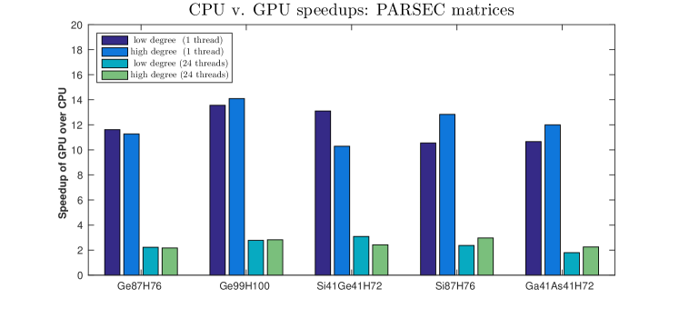
Figure 4 shows the speedup of the GPU FLP implementation over the CPU-based counterpart. The CPU results were obtained by executing the FILTLAN software package on the Mesabi linux cluster at University of Minnesota Supercomputing Institute. Mesabi consists of 741 nodes of various configurations with a total of 17,784 compute cores provided by Intel Xeon E5-2680 v3 processors. Each node features two sockets, each socket with twelve physical cores, and each core with a clock speed of 2.50 GHz. Each node is also equipped with 64 GB of RAM memory. The FILTLAN package has the option to link the Intel Math Kernel Library (MKL) when it, as well as a compatible Intel compiler are available. For these experiments we used the Intel compiler icpc version 11.3.2.
We have divided the comparison into four parts: a “low degree” situation when ( for Ga41As41H72), and a “high degree” situation when ( for Ga41As41H72) and within each of these we also executed FILTLAN using both thread and threads. The multithreading was handled entirely by the MKL. In the single thread case, the GPU implementation obtains a speedup which ranges between and . In the thread case, which corresponds to one thread per core on this machine, the speedups ranged between and .
5 Conclusion
In this work we presented a GPU implementation of the filtered Lanczos procedure for solving large and sparse eigenvalue problems such as those that arise from real-space DFT methods in electronic structure calculations. Our experiments indicate that the use of GPU architectures in the context of electronic structure calculations can provide a speedup of at least a factor of over a single core CPU implementation and at least of factor of for a core implementation.
Possible future research directions include the utilization of more than one GPU to perform the filtered Lanczos procedure in computing environments with access to multiple GPUs. Each GPU can then be used to either perform the sparse matrix-vector products and other operations of the FLP in parallel, or compute all eigenpairs in a sub-interval of the original interval. In the later case the implementation proposed in this paper can be used without any modifications. Another interesting extension would be to use additional customization and add support for other sparse matrix formats. A dense matrix version of the proposed implementation would also be of interest for solving sequences of eigenvalue problems as in [49].
References
- [1] H. Fang, Y. Saad, A filtered Lanczos procedure for extreme and interior eigenvalue problems, SIAM J. Sci. Comp. 34 (2012) A2220–A2246.
- [2] C. Lanczos, An iteration method for the solution of the eigenvalue problem of linear differential and integral operators, J. Res. Nat. Bur. Standards 45 (1950) 255–282.
- [3] G. Schofield, J. R. Chelikowsky, Y. Saad, A spectrum slicing method for the Kohn–Sham problem, Comput. Phys. Commun. 183 (2012) 497 – 505.
- [4] Y. Zhou, A block Chebyshev-Davidson method with inner-outer restart for large eigenvalue problems, J. Comput. Phys. 229 (24) (2010) 9188 – 9200.
- [5] Y. Zhou, Y. Saad, A Chebyshev-Davidson algorithm for large symmetric eigenproblems, SIAM J. Matrix Anal. Appl. 29 (3) (2007) 954–971.
- [6] Y. Zhou, Y. Saad, M. L. Tiago, J. R. Chelikowsky, Self-consistent-field calculations using Chebyshev-filtered subspace iteration, J. Comput. Phys. 219 (1) (2006) 172 – 184.
- [7] Y. Saad, A. Stathopoulos, J. Chelikowsky, K. Wu, S. Öǧüt, Solution of large eigenvalue problems in electronic structure calculations, BIT 36 (3) (1996) 563–578.
- [8] P. Hohenberg, W. Kohn, Inhomogeneous electron gas, Phys. Rev. 136 (1964) B864–B871.
- [9] W. Kohn, L. J. Sham, Self-consistent equations including exchange and correlation effects, Phys. Rev. 140 (1965) A1133–A1138.
- [10] J. R. Chelikowsky, Y. Saad, I. Vasiliev, Atoms and clusters, in: Time-Dependent Density Functional Theory, Vol. 706 of Lecture notes in Physics, Springer-Verlag, Berlin, Heidelberg, 2006, Ch. 17, pp. 259–269.
- [11] W. R. Burdick, Y. Saad, L. Kronik, M. Jain, J. R. Chelikowsky, Parallel implementations of time-dependent density functional theory, Comput. Phys. Commun. 156 (2003) 22–42.
- [12] V. Kalantzis, A GPU implementation of the filtered Lanczos algorithm for interior eigenvalue problems (2015).
- [13] J. L. Aurentz, GPU accelerated polynomial spectral transformation methods, Ph.D. thesis, Washington State University (2014).
- [14] K. Wu, H. Simon, Thick-restart Lanczos method for large symmetric eigenvalue problems, SIAM J. Matrix Anal. Appl. 22 (2) (2000) 602–616.
- [15] J. Baglama, D. Calvetti, L. Reichel, IRBL: An implicitly restarted block-Lanczos method for large-scale hermitian eigenproblems, SIAM J. Sci. Comp. 24 (5) (2003) 1650–1677.
- [16] D. Calvetti, L. Reichel, D. C. Sorensen, An implicitly restarted Lanczos method for large symmetric eigenvalue problems, Electron. Trans. Numer. Anal. 2 (1) (1994) 21.
- [17] J. Cullum, W. E. Donath, A block Lanczos algorithm for computing the algebraically largest eigenvalues and a corresponding eigenspace of large, sparse, real symmetric matrices, in: Decision and Control including the 13th Symposium on Adaptive Processes, 1974 IEEE Conference on, IEEE, 1974, pp. 505–509.
- [18] C. C. Paige, The computation of eigenvalues and eigenvectors of very large sparse matrices, Ph.D. thesis, University of London (1971).
- [19] D. C. Sorensen, Implicitly restarted Arnoldi/Lanczos methods for large scale eigenvalue calculations, Tech. rep. (1996).
- [20] C. A. Beattie, M. Embree, D. C. Sorensen, Convergence of polynomial restart krylov methods for eigenvalue computations, SIAM Rev. 47 (3) (2005) 492–515.
- [21] R. B. Lehoucq, Analysis and implementation of an implicitly restarted Arnoldi iteration, Ph.D. thesis, Rice University (1995).
- [22] Y. Saad, On the rates of convergence of the Lanczos and the block-Lanczos methods, SIAM J. Numer. Anal. 17 (5) (1980) 687–706.
- [23] H. D. Simon, The Lanczos algorithm with partial reorthogonalization, Math. Comp. 42 (165) (1984) 115–142.
- [24] Y. Saad, Numerical Methods for Large Eigenvalue Problems, Second Edition, SIAM, Philadelphia, PA, USA, 2011.
- [25] D. S. Watkins, The Matrix Eigenvalue Problem: and Krylov Subspace Methods, SIAM, Philadelphia, PA, USA, 2007.
- [26] C. Bekas, E. Kokiopoulou, Y. Saad, Computation of large invariant subspaces using polynomial filtered Lanczos iterations with applications in density functional theory, SIAM J. Matrix Anal. Appl. 30 (1) (2008) 397–418.
- [27] L. O. Jay, H. Kim, Y. Saad, J. R. Chelikowsky, Electronic structure calculations for plane-wave codes without diagonalization, Comput. Phys. Commun. 118 (1) (1999) 21–30.
- [28] Y. Saad, Filtered conjugate residual-type algorithms with applications, SIAM J. Matrix Anal. Appl. 28 (3) (2006) 845–870.
- [29] R. N. Silver, H. Roeder, A. F. Voter, J. D. Kress, Kernel polynomial approximations for densities of states and spectral functions, J. Comput. Phys. 124 (1) (1996) 115–130.
- [30] A. Weiße, G. Wellein, A. Alvermann, H. Fehske, The kernel polynomial method, Rev. Modern Phys. 78 (1) (2006) 275.
- [31] D. Jackson, The Theory of Approximation, Vol. 11 of Colloquium publications, AMS, New York, NY, USA, 1930.
- [32] C. W. Clenshaw, A note on the summation of Chebyshev series, Math. Tab. Wash. 9 (1955) 118–120.
- [33] N. Corporation, NVIDIA CUDA C Programming Guide, v7.0 Edition (October 2015).
- [34] J. L. Aurentz, V. Kalantzis, Y. Saad, Cucheb, https://github.com/jaurentz/cucheb (2016).
- [35] J. Nickolls, I. Buck, M. Garland, K. Skadron, Scalable parallel programming with cuda, Queue 6 (2) (2008) 40–53.
- [36] R. F. Boisvert, R. Pozo, K. Remington, R. F. Barrett, J. J. Dongarra, Matrix market: A web resource for test matrix collections, in: Proceedings of the IFIP TC2/WG2.5 Working Conference on Quality of Numerical Software: Assessment and Enhancement, Chapman & Hall, Ltd., London, UK, UK, 1997, pp. 125–137.
- [37] T. A. Davis, Y. Hu, The University of Florida sparse matrix collection, ACM Trans. Math. Software 38 (1) (2011) 1–25.
- [38] I. Reguly, M. Giles, Efficient sparse matrix-vector multiplication on cache-based gpus, in: Innovative Parallel Computing, IEEE, 2012, pp. 1–12.
- [39] N. Bell, M. Garland, Implementing sparse matrix-vector multiplication on throughput-oriented processors, in: SC ’09: Proc. Conference on High Performance Computing Networking, Storage and Analysis, 2009.
- [40] N. Corporation, CUSPARSE Library User Guide, v7.0 Edition (October 2015).
- [41] W. E. Arnoldi, The principle of minimized iterations in the solution of the matrix eigenvalue problem, Quart. Appl. Math. 9 (1) (1951) 17–29.
- [42] B. N. Parlett, The Symmetric Eigenvalue Problem, SIAM, Philadelphia, PA, USA, 1980.
- [43] N. Corporation, CUBLAS Library User Guide, v7.0 Edition (October 2015).
- [44] B. N. Parlett, D. S. Scott, The Lanczos algorithm with selective orthogonalization, Math. Comp. 33 (145) (1979) 217–238.
- [45] H. D. Simon, Analysis of the symmetric Lanczos algorithm with reorthogonalization methods, Linear Algebra Appl. 61 (1984) 101–131.
- [46] L. Kronik, A. Makmal, M. L. Tiago, M. M. G. Alemany, M. Jain, X. Huang, Y. Saad, J. R. Chelikowsky, PARSEC–the pseudopotential algorithm for real-space electronic structure calculations: recent advances and novel applications to nano-structures, Phys. Status Solidi (B) 243 (5) (2006) 1063–1079.
- [47] V. Kalantzis, J. Kestyn, E. Polizzi, Y. Saad, Domain decomposition contour integration approaches for symmetric eigenvalue problems (2016).
- [48] V. Kalantzis, R. Li, Y. Saad, Spectral Schur complement techniques for symmetric eigenvalue problems, Electron. Trans. Numer. Anal. 45 (2016) 305–329.
- [49] M. Berljafa, D. Wortmann, E. Di Napoli, An optimized and scalable eigensolver for sequences of eigenvalue problems, Concurr. Comput. 27 (4) (2015) 905–922.