Center vortices and localized Dirac modes in the deconfined phase of 2+1 dimensional lattice $\mathbb{Z}_{2}$ gauge theory

Abstract

We study the deconfinement transition in 2+1 dimensional lattice $\mathbb{Z}_{2}$ gauge theory both as a percolation transition of center vortices and as a localization transition for the low-lying Dirac modes. We study in detail the critical properties of the Anderson transition in the Dirac spectrum in the deconfined phase, showing that it is of BKT type; and the critical properties of the center-vortex percolation transition, showing that they differ from those of ordinary two-dimensional percolation. We then study the relation between localized modes and center vortices in the deconfined phase, identifying the simple center-vortex structures that mainly support the localized Dirac modes. As the system transitions to the confined phase, center vortices merge together into an infinite cluster, causing the low Dirac modes to delocalize.

I Introduction

A growing amount of evidence shows that the localization properties of low-lying Dirac modes in a gauge theory are strongly connected with its confining properties: Low Dirac modes, while extended in the confined phase of a gauge theory, become localized in the deconfined phase, exactly at the critical temperature when this corresponds to a genuine phase transition [1, 2, 3, 4, 5, 6, 7, 8, 9, 10, 11, 12, 13, 14, 15, 16, 17, 18, 19, 20, 21, 22, 23] (see Ref. [24] for a recent review). More precisely, in the deconfined phase the localized low Dirac modes are separated from the delocalized bulk modes by a critical point in the spectrum known as “mobility edge”. At the mobility edge the localization length diverges and a phase transition along the spectrum, known as Anderson transition [25, 26, 27, 28, 29], takes place. As one crosses over to the confined phase, the mobility edge vanishes (possibly discontinuously [17, 16]), and localized modes disappear from the spectrum. While the existence of a relation between localization and deconfinement is by now established, the nature of this relation has not been fully elucidated yet.

The connection between deconfinement and localization of low Dirac modes in gauge theories is qualitatively understood in terms of the “sea/islands” picture proposed in Ref. [5] and further developed in Refs. [30, 31, 32, 24, 20]. In the “physical sector” where Polyakov loops order along 1, selected by dynamical fermions or, in the case of pure gauge theories, by (infinitely) heavy external fermionic probes, a pseudogap opens in the Dirac spectrum due to the ordering of the Polyakov loop. In the resulting “sea” of ordered local Polyakov loops, gauge-field fluctuations that reduce the correlation across time slices, such as Polyakov-loop fluctuations away from 1, are localized on “islands”, typically well-separated in space. These fluctuations reduce the ability of Dirac modes to diffuse in space, and can “trap” the Dirac modes if these develop an eigenvalue below the gap, localizing the corresponding eigenvectors. This mechanism clearly applies not only in a deconfined phase, but more generally when the Polyakov loop gets ordered, e.g., in the Higgs phase of the $\mathrm{SU}(2)$ Higgs model [22].

The connection between localization and deconfinement shows up even in the simplest gauge theory with a deconfining transition, namely pure $\mathbb{Z}_{2}$ gauge theory in 2+1 dimensions [19]. This model is dual to an anisotropic three-dimensional Ising model [33] (summed over boundary conditions: see Refs. [34, 35] and references therein, and Ref. [20] for a detailed derivation), which allows for an accurate determination of the critical value of the gauge coupling [34] through the use of a cluster algorithm [36, 37]. While localization of low Dirac modes was clearly demonstrated in Ref. [19], a precise determination of the mobility edge and of its temperature dependence, as well as a detailed study of the corresponding Anderson transition, were not undertaken.

Gauge configurations in an Abelian model like the $\mathbb{Z}_{2}$ theory are entirely determined by the simplest plaquettes and by the Polyakov loops in the various directions, with those along the spatial ones becoming irrelevant in the large-volume limit. In the $\mathbb{Z}_{2}$ theory, plaquette configurations on the direct lattice are in one-to-one correspondence with configurations of closed loops on the dual lattice, constructed by associating an “active” dual link to each nontrivial plaquette. Dual loops can further intersect each other, and are conveniently grouped in disconnected clusters of various sizes. Since the gauge group is Abelian and so equal to its own center, these clusters are trivially the same as the center vortices of this model, so we will refer to them also as center vortices in the following (for recent results on center vortices in QCD and a list of references, see Ref. [38]).

Clearly, the sum of the sizes of these clusters equals the number of negative plaquettes of the gauge configuration on the direct lattice, and one can exactly recast the partition function in terms of dual clusters. The dynamics of $\mathbb{Z}_{2}$ gauge fields is then the dynamics of center vortices. In this language, confinement can be understood as center-vortex percolation, i.e., as the formation of a percolating cluster of dual active links, that leads to a nonvanishing string tension. Conversely, deconfinement corresponds to the disappearance of the percolating cluster, with only clusters of finite size surviving the large-volume limit. The idea of looking at the confinement/deconfinement transition as a center-vortex percolation transition was proposed in Ref. [39] for the pure $\mathrm{SU}(2)$ gauge theory. Reference [40] studied instead $\mathbb{Z}_{2}$ gauge theory in 2+1 dimensions, showing the presence of an infinite center-cluster in typical gauge configurations in the confined phase, and demonstrating its crucial role in establishing confinement. On the other hand, the behavior of clusters across the deconfinement transition was not investigated.

Pure $\mathbb{Z}_{2}$ gauge theory in 2+1 dimensions is clearly the easiest setup in which one can study the nature of the gauge-field fluctuations relevant to localization, and how these relate to the confining properties of the theory. In particular, the connection between deconfinement and localization on the one hand, and that between confinement and percolation on the other, suggests that the features of the non-percolating center clusters expected in the deconfined phase should play an important role for localization. Identifying the features of gauge-field configurations that connect localization and deconfinement in this simple model may lead to further insight on the problem of confinement in the physically relevant case of QCD, and more generally in non-Abelian gauge theories.

In this paper we investigate in detail the localization of Dirac modes, the percolation of center vortices, and how they affect each other in pure $\mathbb{Z}_{2}$ gauge theory in 2+1 dimensions on the lattice, probed with external staggered fermions. After briefly introducing the model, in Sec. II we discuss a few generalities about center vortices and localization. In Sec. III we present our numerical results. We first determine the nature of the Anderson transition and the temperature dependence of the mobility edge. We then study the percolation of center vortices across the deconfinement transition and the correlation between center clusters and localized modes, and test the refined sea/islands picture of Ref. [20]. We then identify the features of center vortices mostly relevant to localization. Finally, in Sec. IV we present our conclusions and discuss prospects for future studies.

II Localization and center vortices in $\mathbb{Z}_{2}$ lattice gauge theory at finite temperature

In this Section, after briefly describing 2+1-dimensional pure $\mathbb{Z}_{2}$ gauge theory on the lattice and how to probe it with external staggered fermions, we summarize the relevant aspects of center vortices and their percolation, and of Dirac mode localization.

II.1 Finite-temperature $\mathbb{Z}_{2}$ lattice gauge theory in 2+1 dimensions

We consider pure $\mathbb{Z}_{2}$ gauge theory on a 2+1-dimensional hypercubic $N_{t}\times N_{s}^{2}$ lattice. Lattice sites are denoted by $n=(n_{1},n_{2},n_{3})=(t,\vec{x})$, where $0\leq t=n_{1}\leq N_{t}-1$, $0\leq x_{1,2}=n_{2,3}\leq N_{s}-1$. The dynamical variables of the model are the link variables $U_{\mu}(n)=\pm 1$, taking values in $\mathbb{Z}_{2}$, and associated with the oriented lattice links connecting a site $n$ with its neighbors $n+\hat{\mu}$, where $\mu=1,2,3$ and $\hat{\mu}$ is the unit lattice vector in direction $\mu$. Periodic boundary conditions are imposed in all directions.

The relevant gauge-invariant observables are the plaquette variables $U_{\mu\nu}(n)$ associated with the elementary lattice squares,

$$U_{\mu\nu}(n) \equiv U_{\mu}(n)U_{\nu}(n+\hat{\mu})U_{\mu}(n+\hat{\nu})^{-1}U_{\nu}(n)^{-1}$$ (1)

$$=U_{\mu}(n)U_{\nu}(n+\hat{\mu})U_{\mu}(n+\hat{\nu})U_{\nu}(n)\,,$$

and the Polyakov loops winding around the temporal direction,

$$P(\vec{x})\equiv\prod_{t=0}^{N_{t}-1}U_{1}(t,\vec{x})\,.$$ (2)

Together with the analogues of $P(\vec{x})$ winding around the spatial directions, these quantities determine the link configuration up to a gauge transformation.

Expectation values of observables $O[U]$ are defined as

$$\langle O[U]\rangle =Z^{-1}\sum_{\{U_{\mu}(n)=\pm 1\}}e^{-S[U]}\,O[U]\,,$$ (3)

$$Z =\sum_{\{U_{\mu}(n)=\pm 1\}}e^{-S[U]}\,,$$

where $Z$ is the partition function, the sum is over all possible gauge configurations $\{U_{\mu}(n)\}$, and $S$ is taken to be the Wilson action, which for this model reads (up to an irrelevant additive constant)

$$S[U]=-\beta\sum_{n}\sum_{\begin{subarray}{c}\mu,\nu=1\\ \mu<\nu\end{subarray}}^{3}U_{\mu\nu}(n)\,,$$ (4)

where $\beta$ is the dimensionless lattice coupling, $\beta=1/(e^{2}a)$, with $e$ the coupling constant of mass dimension $1/2$ and $a$ the lattice spacing.

We work at finite temperature $T=1/(aN_{t})$, taking the thermodynamic limit by sending the lattice volume $V=N_{s}^{2}\to\infty$ at fixed $N_{t}$. We set the temperature by varying $\beta$ at fixed $N_{t}$, so in this approach the lattice coupling and the temperature are essentially identified, i.e., $T/e^{2}=\beta/N_{t}$ (up to scaling violations that we ignore for simplicity). The system undergoes a second-order phase transition at a critical coupling $\beta_{c}=\beta_{c}(N_{t})$, from a low-temperature confined phase ($\beta<\beta_{c}$) to a high-temperature deconfined phase ($\beta>\beta_{c}$). The values of $\beta_{c}$ for several temporal sizes in lattice units have been determined in Ref. [34] exploiting the duality with the three-dimensional Ising model. In the deconfined phase the $\mathbb{Z}_{2}$ center symmetry is spontaneously broken; we select the sector where $P(\vec{x})$ prefers the value 1 (physical sector), i.e., configurations where the spatially averaged Polykov loop $\bar{P}\equiv\frac{1}{V}\sum_{\vec{x}}P(\vec{x})$ is positive.

II.2 Staggered Dirac spectrum

We probe the gauge-field configurations using external fermion fields by studying the spectrum of the staggered Dirac operator, which for 2+1 dimensional gauge theories reads

$$D^{\rm stag}=\frac{1}{2}\sum_{\mu=1}^{3}\eta_{\mu}(U_{\mu}T_{\mu}-T_{\mu}^{\dagger}U_{\mu}^{\dagger})\,,$$ (5)

where $T_{\mu}$ are translation operators, $(T_{\mu})_{n,n^{\prime}}=\delta_{n+\hat{\mu},n^{\prime}}$, with periodic boundary conditions in the spatial directions and antiperiodic boundary conditions in the temporal direction, $(U_{\mu})_{n,n^{\prime}}=U_{\mu}(n)\delta_{n,n^{\prime}}$, and $(\eta_{\mu})_{n,n^{\prime}}=\eta_{\mu}(n)\delta_{n,n^{\prime}}$ with $\eta_{\mu}(n)=(-1)^{\sum_{\nu<\mu}n_{\nu}}$. Of course, for $\mathbb{Z}_{2}$ gauge fields $U_{\mu}^{\dagger}=U_{\mu}^{*}=U_{\mu}$. The spectrum of $D^{\rm stag}$ is purely imaginary thanks to the anti-Hermiticity of $D^{\rm stag}$,

$$D^{\rm stag}\psi_{l}=i\lambda_{l}\psi_{l}\,,\qquad\lambda_{l}\in\mathbb{R}\,,$$ (6)

where the eigenvectors $\psi_{l}$ are normalized as usual, $\sum_{n}|\psi_{l}(n)|^{2}=1$. The spectrum is also symmetric about zero since

$$D^{\rm stag}\varepsilon\psi_{l} =-i\lambda_{l}\varepsilon\psi_{l}\,,$$ (7)

$$(\varepsilon)_{n^{\prime}n} =\varepsilon(n)\delta_{n^{\prime}n}\,,\qquad\varepsilon(n)\equiv(-1)^{\sum_{\mu=1}^{3}n_{\mu}}\,,$$

so it suffices to focus on the positive spectrum only. Notice that for free staggered fermions the eigenvalues are

$$\lambda^{\mathrm{free}}(\omega,\vec{p}\,)=\pm\sqrt{(\sin\omega)^{2}+(\sin p_{1})^{2}+(\sin p_{2})^{2}}\,,$$ (8)

where $\omega=\frac{(2k_{0}+1)\pi}{N_{t}}$ with $k_{0}=0,\ldots,N_{t}-1$ are the Matsubara frequencies of the system, and $\vec{p}=(p_{1},p_{2})=\frac{2\pi\vec{k}}{N_{s}}$ with $k_{1,2}=0,\ldots,N_{s}-1$ are the allowed spatial momenta (in lattice units). The positive spectrum is then entirely contained in the finite interval $[\lambda_{(0)},\lambda_{(1)}]$ with $\lambda_{(0)}=\sin\omega_{0}$ and $\lambda_{(1)}=\sqrt{\max_{k}(\sin\omega_{k})^{2}+2}$. We will refer to this region as the bulk of the spectrum, and to modes in the regions $0\leq\lambda<\lambda_{(0)}$ and $\lambda_{(1)}<\lambda\leq 3$ as low and high modes, respectively.

Observables related to the spectrum and the eigenvectors of $D^{\mathrm{stag}}$ are computed locally in the spectrum by averaging within (in principle infinitesimal) spectral bins and over configurations,

$$\overline{O}(\lambda;N_{s})\equiv\frac{\langle\sum_{l}\delta(\lambda-\lambda_{l})O_{l}\rangle}{\langle\sum_{l}\delta(\lambda-\lambda_{l})\rangle}\,,$$ (9)

where $O_{l}$ denotes any eigenmode observable evaluated for mode $l$, and we have made explicit the dependence of the average on the spatial size $N_{s}$ of the system. The numerator in Eq. (9) is the spectral density, i.e., the local density of modes, that grows proportionally to the lattice volume. The suitably normalized spectral density,

$$\rho(\lambda)\equiv\frac{1}{N_{t}V}\left\langle{\textstyle\sum_{l}}\delta(\lambda-\lambda_{l})\right\rangle\,,$$ (10)

has then a well-defined thermodynamic limit. Finally, we define the scaling dimension $d_{O}$ of the spectral quantities $\overline{O}(\lambda;N_{s})$ via

$$d_{O}(N_{s}^{\prime},N_{s}) =\log\frac{\overline{O}(\lambda;N_{s}^{\prime})}{\overline{O}(\lambda;N_{s})}\bigg{/}\log\frac{N_{s}^{\prime}}{N_{s}}\,,$$ (11)

$$d_{O} =\lim_{\begin{subarray}{c}N_{s},N_{s}^{\prime}\to\infty\\ N_{s}\neq N_{s}^{\prime}\end{subarray}}d_{O}(N_{s}^{\prime},N_{s})\,.$$

II.3 Center vortices

The sum over the configurations of link variables $U_{\mu}(n)$ defining the partition function of $\mathbb{Z}_{2}$ gauge theory defines also a percolation problem for the plaquette variables $U_{\mu\nu}(n)$. This is most easily formulated on the dual lattice, where each dual link corresponds to one elementary lattice square on the direct lattice, namely the one it pierces in its center. One then defines a dual lattice link variable equal to the plaquette variable on the corresponding direct lattice square. “Active bonds”, i.e., negative dual link variables, must form closed loops: since $\mathbb{Z}_{2}$ is Abelian, the product of the plaquettes surrounding every elementary direct-lattice cube must equal one, and so an even number of active dual links must meet at each dual-lattice site. These closed, possibly self-intersecting loops provide an unambiguous definition of clusters of dual links, disconnected from each other. In turn, the sites touched by the dual links in such a cluster form an unambiguously and uniquely identified cluster of dual sites. We will then refer to the union of a dual-link cluster and the associated dual-site cluster simply as a cluster, or as a center vortex.

One can then ask if in typical gauge configurations one finds an infinite center vortex, i.e., a cluster whose size grows linearly with the lattice volume. This is the percolation problem we are interested in. As argued in Ref. [39], the presence of such a cluster would lead to a finite string tension and so to a confining theory. The cluster size can be measured by the number of links, or alternatively by the number of sites it contains. We choose the latter, and denote with $\mathcal{S}$ the fraction of dual sites occupied by the largest cluster in a given gauge configuration, i.e.,

$$\mathcal{S}=\frac{\text{n.~{}of dual sites in the largest cluster}}{N_{t}\times N_{s}^{2}}\,.$$ (12)

The expectation value of $\mathcal{S}$ depends on the lattice coupling $\beta$ through the probability $\alpha$ of activating a dual-lattice link, that in turn equals the probability of finding a negative plaquette on the direct-lattice gauge configuration, i.e.,

$$\alpha\equiv\frac{1-\langle U_{\mu\nu}\rangle}{2}\,.$$ (13)

This quantity sets the concentration of active bonds in the corresponding percolation problem. Notice that the use of periodic boundary conditions in space and the topological constraints on the bond configurations make it a different problem from usual percolation in two dimensions.

To study the correlation between center vortices, defined on the dual lattice, and staggered eigenmodes, defined on the direct lattice, one can proceed as follows. For each dual-link cluster $C$ we define a corresponding size $S(C)$ on the direct lattice by counting the number of sites of the direct lattice touched by the negative plaquettes corresponding to the dual links belonging to $C$. If a site $n$ on the direct lattice is touched by negative plaquettes belonging to $N$ different clusters, we add a contribution $s(n,C)=1/N$ to the size of each of the $N$ clusters; otherwise we set $s(n,C)=0$. In formulas,

$$S(C)=\sum_{n}s(n,C)\,.$$ (14)

We then measure the weight $W(l,C)$ of the $l$th eigenmode on cluster $C$ by adding up the amplitude squared $|\psi_{l}(n)|^{2}$, weighted by the contribution $s(n,C)$ of $n$ to the cluster,

$$W(l,C)=\sum_{n}|\psi_{l}(n)|^{2}s(n,C)\,.$$ (15)

For each mode $\psi_{l}$ we then identify the cluster $C_{\mathrm{max}}(l)$ carrying the largest fraction of the mode’s weight, i.e.,

$$\max_{C}W(l,C)=W(l,C_{\mathrm{max}}(l))=W_{\mathrm{max}}(l)\,.$$ (16)

The size of this mode is denoted with $S_{\mathrm{max}}(l)=S(C_{\mathrm{max}}(l))$. The density of mode $l$ on this cluster is denoted with

$$D_{\mathrm{max}}(l)=\frac{W_{\mathrm{max}}(l)}{S_{\mathrm{max}}(l)}\,.$$ (17)

To estimate on how many clusters a mode is concentrated, we use the “cluster IPR”, defined as

$$\mathrm{IPR}_{\mathrm{clust}}(l)=\frac{\sum_{C}W(l,C)^{2}}{\left(\sum_{C}W(l,C)\right)^{2}}\,.$$ (18)

In fact, for a mode whose weight on negative plaquettes lies entirely in a single cluster, $\mathrm{IPR}_{\mathrm{clust}}=1$. For a mode whose weight on negative plaquettes is spread out evenly on $N$ clusters, one finds instead $\mathrm{IPR}_{\mathrm{clust}}=1/N$.

II.4 Eigenmode localization

The staggered operator, used here to probe the pure $\mathbb{Z}_{2}$ gauge theory, is technically a random matrix with entries distributed according to the probability distribution of the gauge links implied by the partition function, Eq. (3). Its eigenvalues and eigenvectors are then also random variables, whose statistical properties are studied by averaging over the “disorder realizations” provided by the gauge link configurations.

The localization properties of eigenmodes can be determined from the volume scaling of their inverse participation ratio (IPR) [26, 27, 28, 29],

$$\mathrm{IPR}_{l}\equiv\sum_{n}|\psi_{l}(n)|^{4}\,,$$ (19)

averaged over gauge configurations and over (infinitesimal) spectral bins [see Eq. (9)],

$$\overline{\mathrm{IPR}}(\lambda,N_{s})=\frac{\langle\sum_{l}\delta(\lambda-\lambda_{l})\mathrm{IPR}_{l}\rangle}{\langle\sum_{l}\delta(\lambda-\lambda_{l})\rangle}\,.$$ (20)

If modes in a certain spectral region are delocalized over the entire lattice volume, then $|\psi_{l}(n)|^{2}\sim\frac{1}{VN_{t}}$ and so $\overline{\mathrm{IPR}}\to 0$ as $V\to\infty$. If they are instead localized in a finite spatial region whose typical size $V_{0}$ is independent of the system size, then $|\psi_{l}(n)|^{2}\sim\frac{1}{V_{0}N_{t}}$ inside that region and is negligible outside, and so $\overline{\mathrm{IPR}}$ tends to a finite constant as $V\to\infty$. Instead of $\overline{\mathrm{IPR}}$ it is sometimes convenient to use the average mode size $\overline{\mathrm{IPR}^{-1}}$, or the average participation ratio $\overline{\mathrm{PR}}=\overline{\mathrm{IPR}^{-1}}/(N_{t}V)$, which measures the fraction of the system occupied by the modes. Since $|\psi_{l}(n)|=|\varepsilon(n)\psi_{l}(n)|$, the eigenmodes $\psi_{l}$ and $\varepsilon\psi_{l}$ have the same $\mathrm{IPR}$, and so it suffices to study the positive part of the spectrum.

The localization properties of the eigenvectors of a random matrix are conveniently determined exploiting their connection with the statistical properties of the corresponding eigenvalues [41]. Here we discuss the subject only briefly; a detailed presentation can be found in Ref. [24]. For delocalized modes, the universal statistical properties of the spectrum are expected to be described by the appropriate symmetry class of Random Matrix Theory (RMT) [42, 43]. For localized modes, instead, eigenvalue fluctuations are expected to be described by Poisson statistics [42]. Analytic predictions are available in both cases for the properties of the so-called unfolded spectrum, obtained from the original spectrum by means of a monotonic mapping that makes the (unfolded) spectral density equal to 1 throughout the spectrum,

$$\lambda_{i}\to x_{i}=N_{t}V\int_{\lambda_{\mathrm{min}}}^{\lambda_{i}}d\lambda\,\rho(\lambda)\,,$$ (21)

where the normalized spectral density $\rho(\lambda)$ is defined in Eq. (10). In particular, the probability distribution $p(s)$ of the unfolded level spacings $s_{i}=x_{i+1}-x_{i}$ is known analytically. For Poisson statistics,

$$p_{\rm P}(s)=e^{-s}\,,$$ (22)

while for RMT statistics the corresponding $p_{\rm RMT}$ depends on the symmetry class, and is not available in closed form.

The localization properties of modes in a given spectral region can then be determined by comparing the spectral statistics of the unfolded spectrum of the model, computed locally in the spectrum, with the theoretical predictions: As the system size increases, these observables will tend to the Poisson or RMT theoretical expectation depending on whether the modes are localized or delocalized in the spectral region under consideration. A point in the spectrum separating localized and delocalized modes is known as mobility edge and usually denoted $\lambda_{c}$. At a mobility edge the localization length $\xi$ diverges, typically as a power law, $\xi\sim|\lambda-\lambda_{c}|^{-\nu}$, and the system displays a second-order phase transition along the spectrum known as Anderson transition [25, 26, 27, 28, 29]. This implies that at the mobility edge the spectral statistics are volume-independent. Moreover, one can precisely determine the mobility edge, the critical statistics, and the critical exponent $\nu$ by means of a finite-size-scaling analysis of spectral statistics [44].

In the case at hand, the random matrix of interest is $H=-iD^{\rm stag}$, which is invariant under the anti-unitary transformation $T=\varepsilon K$, where $K$ denotes complex conjugation and $\varepsilon$ is defined in Eq. (7). Since $T^{2}=1$, $H$ belongs to the orthogonal class. The corresponding unfolded level spacing distribution can be approximated quite accurately with the so-called orthogonal Wigner surmise, $p_{\rm WS}$ [42]. An even better approximation is obtained using the family of distributions $p_{\rm B}(s,\omega)$, $\omega\in[0,1]$, known as Brody distributions [45],

$$p_{\rm B}(s,\omega) =a(\omega)s^{\omega}e^{-\frac{a(\omega)}{1+\omega}s^{1+\omega}}\,,$$ (23)

$$a(\omega) =\left[\Gamma\left({\textstyle\frac{1}{1+\omega}}\right)\right]^{1+\omega}(1+\omega)^{-\omega}\,,$$

which interpolates between $p_{\rm P}(s)=p_{\rm B}(s,0)$ and $p_{\rm WS}(s)=p_{\rm B}(s,1)$. In Ref. [46] it was found that the optimal $\omega$ to approximate $p_{\rm RMT}$ is $\omega\approx 0.957\equiv\omega_{0}$ rather than $\omega=1$. Correspondingly, one finds $a(\omega_{0})\simeq 1.546$.

To monitor the transition from localized to delocalized modes, it is convenient to look at observables extracted from the unfolded level spacing distribution, computed locally in the spectrum, and compare them with the theoretical predictions. A useful observable in this context is the integrated probability density [44], $I_{s_{0}}$, that for Brody distributions reads

$$I_{s_{0}}(\omega)=\int_{0}^{s_{0}}ds\,p_{\rm B}(s,\omega)=1-e^{-\frac{a(\omega)}{1+\omega}s_{0}^{1+\omega}}\,.$$ (24)

To maximize the difference between the values of $I_{s_{0}}$ in the Poisson and RMT regimes, one takes $s_{0}\simeq 0.4687$, which is the first crossing point of the exponential distribution and the Brody distribution with $\omega=\omega_{0}$. Correspondingly, one finds $I_{s_{0}\,{\rm RMT}}\simeq I_{s_{0}}(\omega_{0})\simeq 0.1642$, and $I_{s_{0}\,{\rm P}}=I_{s_{0}}(0)\simeq 0.3742$. These values should be compared with the local estimate

$$\overline{I}_{s_{0}}(\lambda,N_{s})=\frac{\langle\sum_{l}\delta(\lambda-\lambda_{l})\theta(s_{0}-s_{l})\rangle}{\langle\sum_{l}\delta(\lambda-\lambda_{l})\rangle}\,.$$ (25)

Anderson transitions observed in certain (spatially) two-dimensional systems in the unitary and orthogonal classes are of Berezinskiĭ-Kosterlitz-Thouless (BKT) type [47, 48, 49, 50, 51, 52, 14], with a localization length diverging exponentially at the mobility edge as

$$\xi\sim\xi_{0}\exp\left\{A|\lambda-\lambda_{c}|^{-\frac{1}{2}}\right\}\,.$$ (26)

Moreover, all points in the spectrum beyond the mobility edge are critical, with volume-independent spectral statistical properties. Indications of this behavior for the $\mathbb{Z}_{2}$ model were found in Ref. [19]. Similar indications were found also in 2+1 dimensional pure $\mathbb{Z}_{3}$ gauge theory in Ref. [20]. The divergence of the localization length shown in Eq. (26) leads one to expect the following scaling behavior for $I_{s_{0}}$ near the mobility edge,

$$\overline{I}_{s_{0}}(\lambda,L)=f\left((\lambda-\lambda_{c})(\log L/L_{0})^{\frac{1}{\nu}}\right)\,,$$ (27)

with $f$ analytic, for $\nu=\frac{1}{2}$, and some constant scale $L_{0}$.

II.5 Sea/islands picture and Dirac-Anderson Hamiltonian

For the staggered Dirac operator the sea/islands picture briefly sketched in the Introduction can be understood more precisely in the language of the Dirac-Anderson Hamiltonian [31, 32, 24, 20]. In $d+1$ dimensions, in the basis where the temporal part of the staggered operator is diagonal, the “Hamiltonian” $-iD^{\mathrm{stag}}$ reads $H^{\rm DA}=-i\Omega^{\dagger}D^{\mathrm{stag}}\Omega$, where $\Omega$ is a suitable unitary change of basis and [20]

$$H^{\rm DA} =\mathcal{E}+\frac{1}{2i}\sum_{j=1}^{d}\eta_{j}\left[\mathcal{V}_{j}T_{j}-T_{j}{}^{\dagger}\mathcal{V}_{j}^{\dagger}\right]\,,$$ (28)

$$\mathcal{E} =\begin{pmatrix}E&\mathbf{0}\\ \mathbf{0}&-E\end{pmatrix}\,,\quad\mathcal{V}_{j}=\begin{pmatrix}A_{j}&B_{j}\\ B_{j}&A_{j}\end{pmatrix}\,,$$

where $E$, $A_{j}$, and $B_{j}$ are $\vec{x}$-dependent $\frac{N_{t}}{2}\times\frac{N_{t}}{2}$ matrices, with $E$ diagonal and $\mathcal{V}_{j}$ unitary, and $T_{j}$ is the translation operator in direction $j$ (with periodic boundary conditions understood), defined under Eq. (5). The matrix $E$ depends only on the local Polyakov loops, while $A_{j}$ and $B_{j}$ are obtained by a discrete temporal Fourier transform of the spatial links, with frequencies related to the local Polyakov loops on neighboring sites. The precise form of the various matrices is given in Ref. [20]. There, it is argued that locations where the $A_{j}$s are larger are found where the correlation among gauge fields on different time slices is reduced, and that they are favorable places for low (and high) modes to live on. Fluctuations reducing the temporal correlation become rare and typically separated in space in the deconfined phase, so they become favorable places for localization. In other words, locations with larger $A_{j}$s provide the islands of the sea/islands picture. To detect them one can use the quantity

$${\cal A}(\vec{x}) \equiv\frac{1}{N_{t}d}\sum_{j=1}^{d}{\rm tr}\,\left\{A_{j}(\vec{x}){}^{\dagger}A_{j}(\vec{x})\right.$$ (29)

$$\hphantom{\equiv\frac{1}{N_{t}d}\sum_{j=1}^{d}{\rm tr}\,}\left.+A_{j}(\vec{x}-\hat{\jmath}){}^{\dagger}A_{j}(\vec{x}-\hat{\jmath})\right\}\,,$$

normalized so that $0\leq{\cal A}(\vec{x})\leq 1$. One can study their correlation with the staggered eigenmodes by measuring ${\cal A}(\vec{x})$ “as seen by the modes” normalized by its average, i.e.,

$${\cal A}_{\psi}(\lambda)\equiv\frac{\left\langle\sum_{l}\delta(\lambda-\lambda_{l})\sum_{\vec{x}}{\cal A}(\vec{x})\sum_{t=0}^{N_{t}-1}|\psi_{l}(t,\vec{x})|^{2}\right\rangle\,,}{\left\langle\sum_{l}\delta(\lambda-\lambda_{l})\right\rangle\langle{\cal A}(\vec{x})\rangle}\,.$$ (30)

It is instructive to study also the correlation between islands and Polyakov loops by using the quantity

$$C_{\mathcal{A}P}\equiv\frac{\left\langle\mathcal{A}(\vec{x})\frac{1-\mathrm{sgn}(\bar{P})P(\vec{x})}{2}\right\rangle}{\left\langle\mathcal{A}(\vec{x})\right\rangle\frac{1-\left\langle|\bar{P}|\right\rangle}{2}}\,.$$ (31)

This measures the average $\mathcal{A}$ on sites where the local Polyakov loop, $P(\vec{x})$, has sign opposite to that of the spatially averaged Polyakov loop, $\bar{P}$, normalized by the average value of $\mathcal{A}$ and by the probability of finding such a Polyakov-loop fluctuation.

III Numerical results

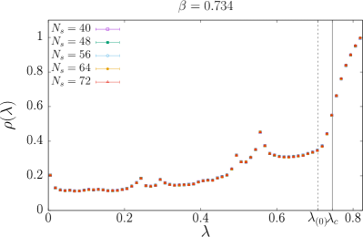
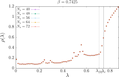
Figure 1: Normalized spectral density $\rho(\lambda)$, Eq. (10), in the deconfined phase at $\beta=0.734$ (top panel) and $\beta=0.7425$ (bottom panel), for $N_{t}=4$ and different spatial system sizes. The low end of the bulk, $\lambda_{(0)}$, and the mobility edge, $\lambda_{c}$, are also shown.

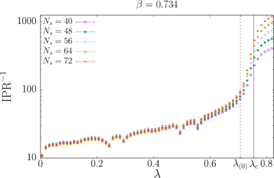
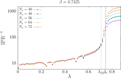
Figure 2: Mode size $\mathrm{IPR}^{-1}$ (in logarithmic scale) at $\beta=0.734$ (top panel) and $\beta=0.7425$ (bottom panel), for $N_{t}=4$ and different spatial system sizes. The low end of the bulk, $\lambda_{(0)}$, and the mobility edge, $\lambda_{c}$, are also shown.

We performed numerical simulations of finite-temperature $\mathbb{Z}_{2}$ gauge theory on hypercubic $N_{t}\times N_{s}^{2}$ lattices with fixed $N_{t}=4$ and several values of $N_{s}$ and $\beta$, using a standard Metropolis algorithm. Details about the values of $N_{s}$ and $\beta$, as well as about the number of generated configurations, are given below. For $N_{t}=4$ the critical coupling separating the confined and deconfined phases is $\beta_{c}=0.73107(2)$ [34], and the bulk of the staggered spectrum is bounded by $\lambda_{(0)}={1}/{\sqrt{2}}$ and $\lambda_{(1)}=\sqrt{{5}/{2}}$ (see above in Sec. II.2).

III.1 Mobility edge

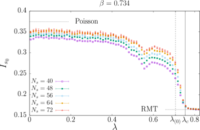
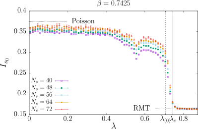
Figure 3: Spectral statistics $I_{s_{0}}$ at $\beta=0.734$ (top panel) and $\beta=0.7425$ (bottom panel), for $N_{t}=4$ and different spatial system sizes. The low end of the bulk, $\lambda_{(0)}$, the mobility edge, $\lambda_{c}$, and the expectations for Poisson and RMT statistics are also shown.

To establish the BKT nature of the Anderson transition and measure the temperature dependence of the mobility edge we performed numerical simulations of the model in the deconfined phase using spatial sizes $N_{s}=40,48,56,64,72$, for $\beta=0.733,0.734,0.735,0.7375,0.74,0.7425$. We generated approximately 86k, 31k, 12k, 6k, and 2.5k configurations for the $N_{s}=40,48,56,64,72$ lattices, respectively. We selected configurations in the physical sector, $\bar{P}=\frac{1}{V}\sum_{\vec{x}}P(\vec{x})>0$; configurations with $\bar{P}<0$ were not discarded, but transformed to a configuration of equal weight with $\bar{P}>0$ by multiplying by $-1$ all the temporal links in the last time slice. We then computed the positive low-lying eigenvalues of the staggered Dirac operator and the corresponding eigenvectors using the ARPACK library [53]. To keep approximately fixed the spectral range and to cover the low-mode region, we increased the number of computed eigenmodes with the system size, obtaining $472,672,920,1200,1520$ modes for $N_{s}=40,48,56,64,72$, respectively.

Numerical estimates $\overline{O}^{\mathrm{num}}$ of the local averages $\overline{O}(\lambda;N_{s})$ of spectral observables $O_{l}$, Eq. (9), are obtained by dividing the spectrum in disjoint intervals ${\cal I}$ of size $\Delta\lambda$ (in lattice units), first averaging $O_{l}$ inside ${\cal I}$ and over configurations to obtain $\overline{O}({\cal I},N_{s})$,

$$\overline{O}({\cal I},N_{s}) \equiv\frac{\langle\sum_{\lambda_{l}\in{\cal I}}O_{l}\rangle}{\mathcal{N}({\cal I},N_{s})}\,,$$ (32)

$$\mathcal{N}({\cal I},N_{s}) \equiv\langle\textstyle\sum_{\lambda_{l}\in{\cal I}}1\rangle\,,$$

and then assigning the result to the average eigenvalue in the interval,

$$\overline{O}^{\mathrm{num}}(\overline{\lambda}({\cal I},N_{s})) \equiv\overline{O}({\cal I},N_{s})\,,$$ (33)

$$\overline{\lambda}({\cal I},N_{s}) =\frac{\langle\sum_{\lambda_{l}\in{\cal I}}\lambda_{l}\rangle}{\mathcal{N}({\cal I},N_{s})}\,.$$

The spectral density is estimated numerically as

$$\rho^{\mathrm{num}}(\overline{\lambda}({\cal I},N_{s}))\equiv\frac{\mathcal{N}({\cal I},N_{s})}{N_{t}V\Delta\lambda}\,.$$ (34)

We estimated statistical errors on these quantities with the jackknife method using 100 jackknife samples.

In Figs. 1 and 2 we show the normalized spectral density $\rho(\lambda)$, Eq. (10), and the average mode size $\overline{\mathrm{IPR}^{-1}}$, see under Eq. (20), along the low-lying spectrum. The spectral density is small but nonzero near $\lambda=0$, and starts to increase rapidly in the bulk, above $\lambda_{(0)}$. In the same region the mode size is essentially volume-independent, indicating localization of the eigenmodes. Peak structures are present in $\rho$ at specific values of $\lambda$ below $\lambda_{(0)}$, where one correspondingly finds dips in the mode size. We will return on this feature below in Sec. III.5.

We then studied the statistical properties of the unfolded spectrum. Since degenerate eigenvalues are absent in the spectral region and for the volumes under consideration, we have obtained the unfolded eigenvalues numerically by sorting in ascending order all the eigenvalues on all the configurations for a given choice of $\beta$ and $N_{s}$, and assigning to each eigenvalue its rank divided by the number of configurations. We then used them to numerically estimate $\overline{I}_{s_{0}}(\lambda,N_{s})$, Eq. (25), as explained above, and studied its volume dependence. The behavior expected for a BKT-type Anderson transitions is clearly visible in Fig. 3, where we show $\overline{I}_{s_{0}}$ for different spatial volumes at $\beta=0.734$ and $\beta=0.7425$ (here $\Delta\lambda=0.0125$). While the low modes tend towards Poissonian statistics as the system size increases, higher up in the spectrum the spectral statistics does not change with $N_{s}$. The lowest Matsubara frequency, $\lambda_{(0)}$, and the mobility edge, $\lambda_{c}$, determined via finite size scaling as discussed below, are also shown. The collapse of the $\overline{I}_{s_{0}}$ curves for different spatial sizes on top of each other starts precisely at $\lambda_{c}$.

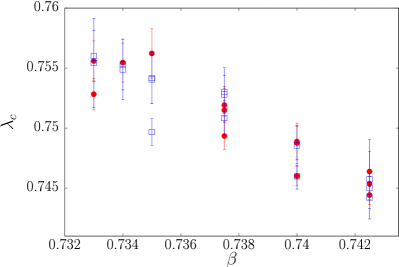
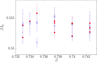
Figure 4: Mobility edge obtained from $I_{s_{0}}$ via a finite size scaling study, in lattice units (top panel) and physical units (bottom panel). Red circles correspond to fits including data from all system sizes, and blue squares to fits exluding data from the smallest size, $L=40$. Different data points at the same $\beta$ correspond to different fitting intervals around the mobility edge.

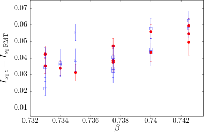
Figure 5: Critical value of $I_{s_{0}}$ at the mobility edge minus the RMT expectation $I_{s_{0}\,{\rm RMT}}\simeq 0.1642$ (top panel), and critical exponent $\nu$ (bottom panel), obtained from $I_{s_{0}}$ via a finite size scaling study. Red circles correspond to fits including data from all system sizes, and blue squares to fits exluding data from the smallest size, $L=40$. Different data points at the same $\beta$ correspond to different fitting intervals around the mobility edge.

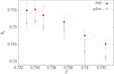
Figure 6: Comparison of the finite size scaling determination of the mobility edge, $\lambda_{c}^{\mathrm{FSS}}$, with the infinite-volume extrapolation of the estimate $\lambda_{c}^{\mathrm{spline}}$, obtained as the intercept of a spline interpolation of numerical data with a prescribed value, as discussed in the text.

We fitted our data for $\overline{I}_{s_{0}}$ (with $\Delta\lambda=0.0075$) to a polynomial truncation of the scaling function Eq. (27), obviously setting $L=N_{s}$, and using the constrained fitting technique of Ref. [54]. This amounts in practice to minimizing an augmented $\chi^{2}_{\mathrm{aug}}=\chi^{2}+\chi^{2}_{\mathrm{prior}}$, where

$$\chi^{2}_{\mathrm{prior}}=\sum_{n}\frac{(c_{n}-\bar{c}_{n})^{2}}{\bar{\sigma}_{n}^{2}}\,,$$ (35)

where the sum extends over the fitting parameters $c_{n}$, and the priors $\bar{c}_{n}$ and $\bar{\sigma}_{n}$ encode our expectations on their value. We used loose priors with a large variance for most of the coefficients, with a few noteworthy exceptions. For $\nu$ we chose $\bar{c}_{\nu}=0.5$ and $\bar{\sigma}_{\nu}=0.05$, which roughly speaking amounts to allowing a 10% deviation from the theoretical expectation. For $\lambda_{c}$ we chose $\bar{c}_{\lambda_{c}}=0.75$ and $\bar{\sigma}_{\lambda_{c}}=0.05$: this is justified by a a qualitative estimate of the point where the $\overline{I}_{s_{0}}$ curves for different spatial sizes collapse on top of each other, that places the mobility edge somewhere in the interval $[0.7,0.8]$ for all the $\beta$ values considered here. Finally, for $L_{0}$ we took both the central value and the variance to be $\bar{c}_{L_{0}}=\bar{\sigma}_{L_{0}}=1$. We then increased the order of the polynomial until the errors on the fit parameters stabilized, monitoring at the same time the value of $\chi^{2}_{\mathrm{aug}}$ per data point: a value of order 1 indicates that the choice of priors is reasonable. We repeated the fit using different fitting ranges around the mobility edge, and including or excluding the smallest volume. We used the MINUIT library [55], and discarded as unsuccessful those fits for which the error on the fitting parameters could not be estimated reliably with the MINOS routine.

Our results for $\lambda_{c}$ are shown in Fig. 4, top panel. The first surprising aspect is that $\lambda_{c}$ exceeds the lowest Matsubara frequency $\lambda_{(0)}$. Localized modes then eat into the bulk of the spectrum, with disorder in the link variables being able to localize modes that one would expect to be extended, instead of modes localized on favorable gauge-field fluctuations becoming delocalized due to mixing with delocalized modes. The second, even more surprising aspect is that $\lambda_{c}$ in lattice units decreases with $\beta$, while in physical units it is compatible with a constant within 1%, see Fig. 4, bottom panel. This suggests that the mobility edge jumps from zero to a finite value at the critical value of the coupling, $\beta_{c}$, unexpectedly since the thermal transition is continuous.

The difference between the critical value of $I_{s_{0}}$ at the mobility edge and the RMT value $I_{s_{0}\,{\rm RMT}}$ is shown in Fig. 5, top panel, and the critical exponent $\nu$ is shown in Fig. 5, bottom panel. Although compatible with a constant behavior within errors, $I_{s_{0}}(\lambda_{c})$ shows an increasing trend with $\beta$. Our estimate of the critical exponent is consistent with the expectation $\nu=\frac{1}{2}$ within errors, although all our estimates but one are below this value.

To check our surprising results for the $\beta$ dependence of $\lambda_{c}$, we estimated the mobility edge using a different approach, less rigorous but also less prone to fit instabilities due to the peculiar nature of the Anderson transition in this system. The idea is that the value of $\lambda$ at which $\overline{I}_{s_{0}}$ takes any prescribed value between the Poisson expectation and the critical value found at $\lambda_{c}$ will eventually tend to the mobility edge as the volume is increased. We then did a spline interpolation $I_{s_{0}}^{\mathrm{spline}}(\lambda)$ of the numerical data for each $\beta$ and $L$, and estimated $\lambda_{c}^{\mathrm{spline}}$ as the solution to $I_{s_{0}}^{\mathrm{spline}}(\lambda_{c}^{\mathrm{spline}}(\beta,L))=0.185$. The specific value on the right hand side of the equation was chosen safely above the (possibly $\beta$-dependent) critical value at the mobility edge, estimated by observing where the curves for the various volumes fall on top of each other at each $\beta$. We then obtained our alternative estimate of the mobility edge by extrapolating to infinite volume, $\lambda_{c}^{\mathrm{spline}}(\beta)=\lim_{L\to\infty}\lambda_{c}^{\mathrm{spline}}(\beta,L)$, assuming a linear dependence on $1/L$. We estimated the systematics from finite size effects by repeating the extrapolation after excluding the smallest volume. For $\beta=0.74$ the result for the largest volume is clearly off of a linear trend, and its inclusion in the fit leads to a very large $\chi^{2}/\mathrm{d.o.f.}$. We have then exluded it from the fit in the determination of the central value, while including the change due to its inclusion in the estimate of the error. In Fig. 6 the results are compared with the average $\lambda_{c}^{\mathrm{FSS}}$ of the determinations of $\lambda_{c}$ via finite size scaling shown in Fig. 4, with total error estimated adding in quadrature the average of the statistical error and the standard deviation over the set of determinations. The two estimates $\lambda_{c}^{\mathrm{FSS}}$ and $\lambda_{c}^{\mathrm{spline}}$ are in agreement within errors, although the alternative estimates is always smaller than the finite size scaling one. This is not entirely surprising, as $\lambda_{c}^{\mathrm{spline}}(\beta,L)$ always underestimates $\lambda_{c}$ by construction, and the linear extrapolation to infinite volume is probably neglecting sizeable effects. In any case, the important aspect is that the two estimates agree on the qualitative behavior of $\lambda_{c}$ as a function of $\beta$.

The decrease of $\lambda_{c}$ with $\beta$ can be understood noticing that the width of the spectral pseudogap, where the density of modes is low, essentially coincides with the lowest Matsubara frequency, which in lattice units depends only on $N_{t}$ and so is fixed here. This makes the low end an effective edge of the spectrum, where disorder localizes the outermost modes first. Increasing $\beta$ at fixed $N_{t}$, the disorder decreases as the system gets more ordered, pushing the mobility edge towards the end of the spectrum, which in this case means reducing $\lambda_{c}$. The decrease in disorder is apparently compensated by the decrease of the lattice spacing $1/\beta=e^{2}a$, so that in physical units the mobility edge stays constant. We return on this point below in Sec. III.4. The difference with other theories studied so far is evident, and presumably due to the discrete nature of the gauge group. In the other cases where the dependence of $\lambda_{c}$ on $\beta$ was studied so far [6, 13, 14, 15, 16, 17, 18, 21], the gauge group was continuous, and in that case probably the spectral pseudogap does not depend only on $N_{t}$ but on $\beta$ as well.

III.2 Center cluster percolation

To study the percolation properties of center clusters across the transition we performed a second set of simulations on lattices with $N_{s}=24,32,40,48,56,64,72,80$, accumulating between 60k and 135k configurations for the various volumes. For each configuration, after counting the number of active bonds, we identified all the center clusters, finding then the largest cluster and measuring its size in terms of the dual sites it touched. We then determined the concentration of active bonds $\alpha$, Eq. (13), and largest cluster density $\mathcal{S}$, Eq. (12), as functions of the lattice coupling $\beta$. Results for $\alpha(\beta)$ for various lattice sizes are shown in Fig. 7, and results for $\mathcal{S}(\beta)$ are shown in Fig. 8. The function $\alpha(\beta)$ is monotonic, and so invertible. At low $\beta$, corresponding to larger active-bond concentrations, $\mathcal{S}(\beta)$ depends mildly on the volume and tends to a finite value as the volume increases, signalling the presence of an infinite cluster.

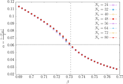
Figure 7: Concentration of active bonds in the percolation problem associated with $\mathbb{Z}_{2}$ gauge theory as a function of the lattice coupling $\beta$, for $N_{t}=4$ and various $N_{s}$. The horizontal dashed lines enclose the confidence band for the critical concentration [see Eq. (37)], while the vertical dashed line marks the deconfinement temperature, $\beta_{c}$ [34].

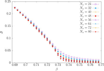
Figure 8: Size of the largest cluster divided by the lattice size, $\mathcal{S}$, Eq. (12), as a function of the lattice coupling $\beta$ for $N_{t}=4$ and various $N_{s}$.

We then studied quantitively the volume scaling of the largest-cluster density $\mathcal{S}$ as a function of the active-bond concentration $\alpha$. To show that the system does indeed undergo a percolation transition, we performed a finite-size scaling analysis of $\mathcal{S}$ as a function of $\alpha$. We fitted our numerical data with the functional form

$$\mathcal{S}(\alpha,L)L^{\frac{\beta}{\nu}}=s((\alpha-\alpha_{c})L^{\frac{1}{\nu}})\,,$$ (36)

truncating the analytic function $s(x)$ to a polynomial of varying order. Here $\beta$ denotes one of the critical exponents, and should not be confused with the lattice coupling. We then used again the constrained fitting techniques of Ref. [54], with very broad priors on Taylor coefficients starting only from the fourth-order one, and using no priors for lower-order coefficients and for the critical concentration $\alpha_{c}$ and critical exponents $\nu$ and $\beta$. Fits were again performed using the MINUIT library [55]. The results of our analysis are summarized in the collapse plot in Fig. 9. The quality of the collapse is excellent. We find for the critical parameters

$$\alpha_{c} =0.06113^{+0.00037}_{-0.00036}\,,$$ (37)

$$\nu =1.431^{+0.012}_{-0.012}\,,$$

$$\frac{\beta}{\nu} =0.637^{+0.013}_{-0.012}\,.$$

The critical exponents clearly deviate from those of two-dimensional percolation (see Ref. [56]). This is probably due to the topological constraint on clusters mentioned above in Sec. II.3, that changes the universality class of the transition.

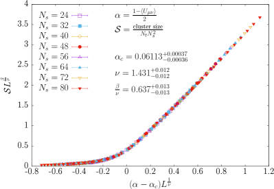
Figure 9: Collapse plot for the rescaled largest-cluster density $\mathcal{S}(\alpha,L)L^{\frac{\beta}{\nu}}$, for $N_{t}=4$ and various $N_{s}$.

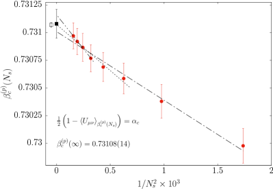
Figure 10: Infinite-volume extrapolation of the critical coupling $\beta_{c}^{(p)}$ for the percolation transition, for $N_{t}=4$. Straight dashed lines correspond to linear extrapolations in $1/N_{s}^{2}$, each ranging only over the volumes used in the extrapolation. The filled black square is our final result for the extrapolation, including statistical and finite-size systematic errors, while the empty black square is the critical lattice coupling for deconfinement obtained in Ref. [34].

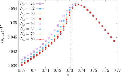
Figure 11: Average number of center clusters $\langle n_{\mathrm{clust}}\rangle$ divided by the lattice spatial volume $V=N_{s}^{2}$ as a function of $\beta$ for various lattice sizes and $N_{t}=4$.

Figure 7 shows that the critical concentration is attained at the deconfinement transition, which corresponds then to the percolation transition for center vortices. To make this statement quantitative, we determined the critical percolation coupling $\beta_{c}^{(p)}$ from the critical concentration $\alpha_{c}$ through the following procedure. For each spatial size $N_{s}$, we define $\beta_{c}^{(p)}(N_{s})$ as the crossing point $\alpha(\beta_{c}^{(p)}(N_{s}))=\alpha_{c}$. This is obtained numerically by means of spline interpolation of $\alpha(\beta)$ and a standard bisection method. Next, we extrapolate $\beta_{c}^{(p)}(N_{s})$ to infinite volume. We performed a linear extrapolation in the inverse volume, fitting $\beta_{c}^{(p)}(N_{s})=a+b/N_{s}^{2}$ including all data, only data for $N_{s}\geq 40$, and only data for $N_{s}\geq 56$, in order to estimate finite-size systematic effects. Results are shown in Fig. 10. We took as central value the average of the three determinations of $a$, as statistical error the average of the statistical errors from the fits, and as systematic error the standard deviation of $a$. The final result is $\beta_{c}^{(p)}=0.73108(12)_{\text{stat}}(06)_{\text{syst}}=0.73108(13)$, in good agreement with the critical coupling $\beta_{c}=0.73107(2)$ for the deconfinement transition found in Ref. [34].

To conclude this Subsection, in Fig. 11 we show how the average number of clusters in a configuration, $\langle n_{\mathrm{clust}}\rangle$, scales with the volume. Deep in the deconfined phase $\langle n_{\mathrm{clust}}\rangle/V$ is clearly constant, showing that the number of clusters grows linearly with the volume. Closer to the transition in the deconfined phase, as well as in the confined phase, the volume scaling seems again to asymptotically approach $n_{\mathrm{clust}}\propto V$, although more slowly. This suggests that a finite density of finite, localized clusters is found also in the confined phase, even in the presence of an infinite cluster.

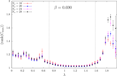
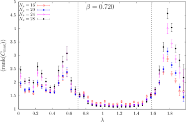
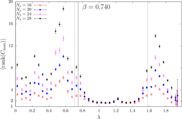
Figure 12: Average rank in magnitude of the cluster $C_{\mathrm{max}}$ on which modes have maximal weight at $\beta=0.69$ (top panel), $\beta=0.72$ (center panel), in the confined phase, and $\beta=0.74$ (bottom panel), in the deconfined phase, for $N_{t}=4$ and various $N_{s}$. Dashed vertical lines mark the ends of the bulk, $\lambda_{(0)}$ and $\lambda_{(1)}$; the solid vertical line in the bottom panel marks the mobility edge $\lambda_{c}$ between low and bulk modes.

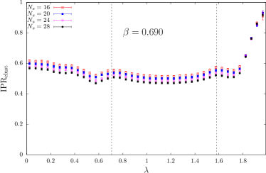
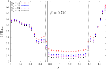
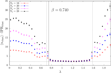
Figure 13: Average cluster IPR, $\mathrm{IPR}_{\mathrm{clust}}$, along the spectrum for $\beta=0.69$ (top panel) and $\beta=0.74$ (center panel), and average $\mathrm{IPR}_{\mathrm{clust}}$ times average number of clusters $\langle n_{\mathrm{clust}}\rangle$ along the spectrum for $\beta=0.74$ (bottom panel), for $N_{t}=4$ and various $N_{s}$. Vertical dashed lines correspond to the bulk ends $\lambda_{(0)}$ and $\lambda_{(1)}$. The solid line in the center and bottom panels corresponds to $\lambda_{c}$. In the bottom panel, the dashed horizontal line corresponds to the value $2$.

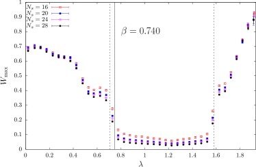
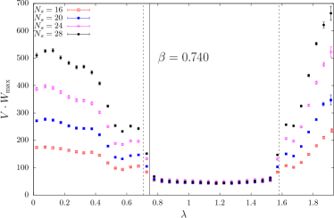
Figure 14: Average maximal weight on a cluster along the spectrum for $\beta=0.69$ (top panel) and $\beta=0.74$ (center panel), and average maximal weight on a cluster times the lattice volume along the spectrum for $\beta=0.74$ (bottom panel), for $N_{t}=4$ and various $N_{s}$. Vertical dashed lines correspond to the bulk ends $\lambda_{(0)}$ and $\lambda_{(1)}$. In the center and bottom panel, the solid line corresponds to $\lambda_{c}$.

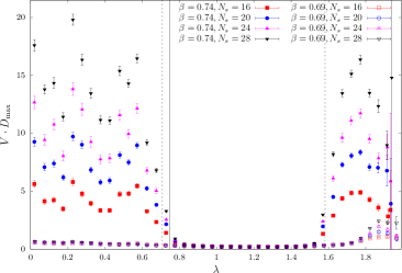
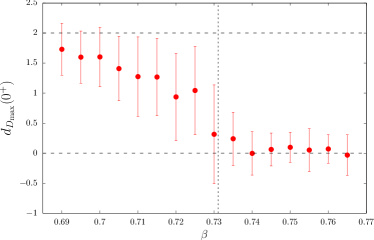
Figure 15: Top panel: Average maximal weight on a cluster divided by the cluster size, $D_{\mathrm{max}}$, computed locally in the spectrum, for $\beta=0.69$ and $\beta=0.74$, for $N_{t}=4$ and various $N_{s}$. Center panel: same quantity as in the top panel but rescaled by the lattice spatial volume $V$. In both panels, vertical dashed lines correspond to the bulk ends $\lambda_{(0)}$ and $\lambda_{(1)}$, and the solid line corresponds to $\lambda_{c}(\beta=0.74)$. Bottom panel: Scaling dimension of $D_{\mathrm{max}}$ [see Eq. (11)] in the lowest spectral bin, averaged over volume pairs. The vertical dashed line corresponds to $\beta_{c}(N_{t}=4)$.

III.3 Correlation between eigenmodes and clusters

We studied the correlation between center vortices and Dirac modes on lattices with $N_{s}=16,20,24,28$, for several $\beta$s across the transition, using 300 configurations for each setup. We identified all center clusters $\{C\}$, and obtained all the staggered modes $\{\psi_{l}\}$ using the LAPACK library [57]. We then measured several types of cross-correlations between the two objects.

In Fig. 12 we show the average rank in magnitude of the cluster $C_{\mathrm{max}}$ on which modes have maximal weight (see Sec. II.3), studied locally in spectrum. At $\beta=0.69$ (top panel), well within the confined phase, this is close to 1 for low and bulk modes, reaching slightly higher values for high modes. This in agreement with the modes’ localization properties: the delocalized low and bulk modes favor the largest cluster, which is the infinite cluster extended over the whole lattice discussed in the previous Subsection, while the localized high modes tend to favor smaller clusters, of lower rank, and more so as the system size increases. At $\beta=0.72$ (center panel), closer to the deconfined phase, low modes start showing a tendency to favor smaller clusters. At $\beta=0.74$ (bottom panel), well within the deconfined phase, the infinite cluster has disappeared, and the relation between the eigenvalue and the average rank of the corresponding $C_{\mathrm{max}}$ is far from straightforward, with the lowest modes not favoring the largest cluster, as one would naively expect, and marked peaks in the low-lying part of the spectrum (already visible, to a lower extent, already in the confined phase).

The cluster IPR, $\mathrm{IPR}_{\mathrm{clust}}$, Eq. (18), averaged locally in the spectrum according to Eq. (9), is shown for $\beta=0.69$ in the confined phase and $\beta=0.74$ in the deconfined phase in the top and center panels of Fig. 13, respectively. At $\beta=0.69$, both low and bulk modes spread on average on $1.5\div 2$ clusters, including the infinite cluster, as shown above, with a mild increase in the spreading as $N_{s}$ increases. Localized high modes instead typically lie on fewer clusters ($1\div 1.5$), without any apparent volume dependence of $\mathrm{IPR}_{\mathrm{clust}}$. This situation changes in the deconfined phase, where the infinite cluster is absent. For bulk modes, $\mathrm{IPR}_{\mathrm{clust}}\simeq 2\langle n_{\mathrm{clust}}\rangle^{-1}$ (see Fig. 13, bottom panel), i.e., they spread on about half of the $n_{\mathrm{clust}}$ (finite) clusters in a configuration; this also determines the marked volume dependence of $\mathrm{IPR}_{\mathrm{clust}}$, since $\langle n_{\mathrm{clust}}\rangle\propto V$, see Fig. 11. Low and high modes, instead, spread on about $1.5\div 3$ and $1\div 3$ clusters, respectively, with a mild volume dependence. This is again in agreement with the modes’ localization properties.

The maximal weight on a cluster $W_{\mathrm{max}}$, Eq. (16), again averaged locally in the spectrum, is shown for the same values of $\beta$ in the top and center panels of Fig. 14. In the confined phase this quantity does not show a big difference between low and bulk modes, and a mild volume dependence for both, reflecting the fact that these modes are delocalized on the infinite center cluster. High modes show a larger value and very little volume dependence, reflecting their localized nature. In the deconfined phase the difference between low and bulk modes becomes marked, and only bulk modes show a noticeable, $1/V$ volume dependence due to their delocalizing over a finite fraction of clusters (see Fig. 14, bottom panel).

Finally, in Fig. 15, top panel, we show the local averages of the density $D_{\mathrm{max}}=W_{\mathrm{max}}/S_{\mathrm{max}}$, Eq. (17), i.e., the mode weight on the cluster carrying the maximal amount of mode weight, divided by the cluster size. This reveals marked peaks at the same points in the spectrum where the spectral density and the mode size also show structures. While these peaks tend to flatten out with increasing volume in the confined phase, they remain essentially constant in the deconfined phase. The volume dependence for bulk modes in both the confined and the deconfined phase is entirely explained by their delocalized nature: a rescaling of $D$ by the spatial volume $V$ makes the curves volume-independent in the bulk region, see Fig. 15, center panel. In the confined phase, low modes still show a mild volume dependence after this rescaling, due to their fractal dimension being smaller than 2 [19]. The scaling dimension $d_{D_{\mathrm{max}}}$ of $D_{\mathrm{max}}$ [see Eq. (11)] in the lowest spectral bin is shown in Fig. 15, bottom panel. Our estimate is obtained averaging over the determinations obtained using different pairs of volumes, and adding in quadrature the average of the corresponding statistical errors and the standard deviation of the determinations to estimate the error. Our results are qualitatively consistent with the nontrivial behavior of the fractal dimension of near-zero modes found in Ref. [19], although $d_{D_{\mathrm{max}}}$ as a function of $\beta$ approaches 2 faster than the fractal dimension as one goes deeper in the confined phase.

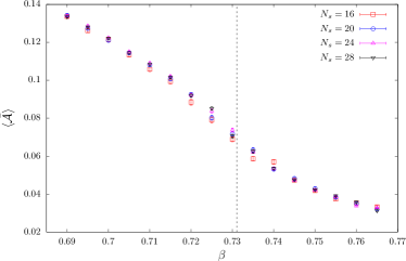
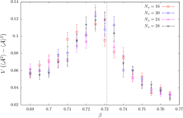
Figure 16: The average $\langle\bar{\mathcal{A}}\rangle$ (top panel) and the susceptibility $V\left(\langle\bar{\mathcal{A}}^{2}\rangle-\langle\bar{\mathcal{A}}\rangle^{2}\right)$ (bottom panel) of $\mathcal{A}(\vec{x})$, for several $\beta$s across the transition, $N_{t}=4$, and various $N_{s}$. The vertical dashed line corresponds to $\beta_{c}(N_{t}=4)$.

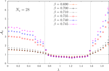
Figure 17: The quantity $\mathcal{A}_{\psi}$, measuring the correlation between islands and eigenmodes, for several values of $\beta$ both in the confined and deconfined phase, on a $28^{2}\times 4$ lattice. Vertical dashed lines correspond to the bulk ends $\lambda_{(0)}$ and $\lambda_{(1)}$.

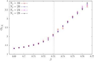
Figure 18: The quantity $O_{C\mathcal{A}}$, Eq. (38), measuring the correlation between center vortices and islands, for several values of $\beta$ both in the confined and deconfined phase, for $N_{t}=4$ and various volumes. The vertical dashed line corresponds to $\beta_{c}$.

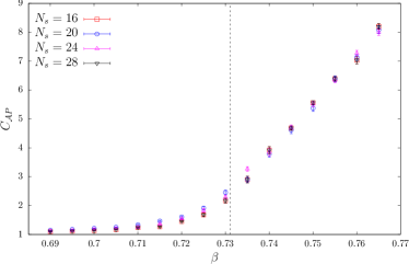
Figure 19: The quantity $C_{\mathcal{A}P}$, Eq. (31), measuring the correlation between Polyakov loops and islands, for several values of $\beta$ both in the confined and deconfined phase, for various volumes. The vertical dashed line corresponds to $\beta_{c}$.

III.4 Refined sea/islands picture

To test the refined sea/islands picture of Ref. [20] we measured the quantity ${\cal A}(\vec{x})$ of Eq. (29) and its correlation with staggered eigenmodes, using the same lattice setups and configurations as in the previous Subsection.

The average of $\bar{\mathcal{A}}\equiv\frac{1}{V}\sum_{\vec{x}}{\cal A}(\vec{x})$ is shown in Fig. 16, top panel. It steadily decreases as $\beta$ increases, indicating that the gauge fluctuations that locally increase the magnitude of $A_{j}$ become less and less frequent as one moves into the deconfined phase, as expected. The susceptibility $V\left(\langle\bar{\mathcal{A}}^{2}\rangle-\langle\bar{\mathcal{A}}\rangle^{2}\right)$ is shown in Fig. 16, bottom panel: it displays a peak near the critical coupling, but does not show a clear scaling with the volume.

The correlation between islands and modes is studied by looking at ${\cal A}_{\psi}$, i.e., ${\cal A}(\vec{x})$ “as seen by the modes” normalized by $\langle{\cal A}\rangle$, Eq. (30). This is shown in Fig. 17. For both low and high modes, ${\cal A}_{\psi}$ is larger than 1 in both phases. In the deconfined phase the ratio shoots up for low modes, showing that they tend to localize where ${\cal A}(\vec{x})$ is larger. High modes are localized already in the confined phase, but for them the ratio shoots up in the deconfined phase even more than for low modes. For bulk modes instead ${\cal A}_{\psi}$ is smaller than 1 in both phases, indicating that these modes are repelled by the islands.

Finally, in Figs. 18 and 19 we show the correlation between islands and center vortices, and between islands and Polyakov loops, respectively. As a measure of the correlation between clusters and islands we used

$$O_{C\mathcal{A}}=\frac{\left\langle\sum_{n}\sum_{\vec{x}}\mathcal{A}(\vec{x})\frac{1}{N_{t}}\sum_{t}\frac{c_{n}(t,\vec{x})}{n_{c}(t,\vec{x})}\right\rangle}{\left\langle\mathcal{A}(\vec{x})\right\rangle\left\langle\sum_{n}\sum_{\vec{x}}\frac{1}{N_{t}}\sum_{t}\frac{c_{n}(t,\vec{x})}{n_{c}(t,\vec{x})}\right\rangle}\,,$$ (38)

where $c_{n}(t,\vec{x})=1$ if the site $(t,\vec{x})$ on the direct lattice is a corner of a plaquette whose corresponding dual link belongs to cluster $n$, and $n_{c}(t,\vec{x})$ is the number of clusters that touch site $(t,\vec{x})$. For the correlation between islands and Polyakov loops we used $C_{\mathcal{A}P}$ defined in Eq. (31), measured on 700 configurations. Both correlations become very strong in the deconfined phase. This strongly suggests that the “islands” relevant to localization are found at the location of those center vortices generated by Polyakov-loop fluctuations away from order.

These results suggest a qualitative explanation for the peculiar dependence of the mobility edge on $\beta$. As already pointed out, the size of the pseudogap is almost equal to $\lambda_{(0)}$, independently of $\beta$, probably due to the discrete nature of the gauge group. Indeed, the diagonal matrix $E$, Eq. (28), has only two, sharply different possible sets of entries, corresponding to sites where $P(\vec{x})=1$ or $P(\vec{x})=-1$. Looking at the hopping, off-diagonal term in the Dirac-Anderson Hamiltonian $H^{\rm DA}$ as a perturbation of the diagonal term, one sees then that unperturbed eigenvectors localized on sites where $P(\vec{x})=-1$ (i.e., on islands) do not mix easily with those localized on sites where $P(\vec{x})=1$ (i.e., in the sea), and so the delocalized region of the spectrum should start from around $\lambda_{(0)}$. Moreover, since avoiding islands likely comes at a cost, one expects the bulk eigenvalues to be pushed further up, increasing the mobility edge above $\lambda_{(0)}$. As the density of islands decreases with increasing $\beta$, their avoidance becomes easier and the mobility edge decreases towards $\lambda_{(0)}$.

III.5 Center vortex structures and localization

As we have already pointed out, the spectral density $\rho$, Fig. 1, shows clear peak structures at specific points in the low part of the spectrum. At the same points, the mode size $\mathrm{IPR}^{-1}$, Fig. 2, shows clear dip structures, indicating correspondingly a stronger localization; and the maximal mode weight on a cluster divided by the cluster size, $D_{\mathrm{max}}$, Fig. 15, also shows clear peaks, indicating a higher concentration of the mode on a single cluster. Structure is visible, although to a much lesser extent, also in other observables, such as $I_{s_{0}}$, Fig. 3, the cluster IPR, $\mathrm{IPR}_{\mathrm{clust}}$, Fig. 13, and the maximal mode weight on a cluster, $W_{\mathrm{max}}$, Fig. 14. These peaks and dips survive, or even become sharper, as the volume increases. As we now show, the presence of these structures in the observables can be traced back to the presence of specific structures in the gauge field, best described in terms of the center vortices they form in the dual lattice.

	object $O$	$\lambda_{O}$	$\tilde{\lambda}_{O}$	$\mathcal{D}_{O}$
	horizontal square	$0.4932906$ $0.5896407$	$1.709904$ $1.628596$	$1$ $4$
	vertical square	$0.5511360$ $0.6697194$	$1.672366$ $1.597334$	$1$ $4$
	flat brick	$0.5462419$	$1.673471$	$2$
	lying brick	$0.5943152$	$1.626896$	$2$
	standing brick	$0.6420283$	$1.646262$	$2$
	chair	$0.2390408$	$1.752455$	$1$
	open book	$0.2928932$	$1.707107$	$1$
	twister	$0$	$\sqrt{3}$	$1$

Table 1: Simplest dual-lattice center-vortex configurations $O$, eigenvalues of the corresponding low ($\lambda_{O}$) and high ($\tilde{\lambda}_{O}$) localized mode (computed on a $4\times 20^{2}$ lattice) and their degeneracy $\mathcal{D}_{O}$. The temporal direction is along the vertical. For the horizontal and vertical square, also the eigenvalues corresponding to their “big”, $2\times 2$ versions are reported on a subsequent line. For the “twister” configuration we found eigenvalues consistent with $0$ and $\sqrt{3}$ within numerical precision.

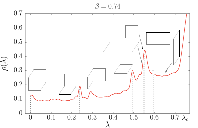
Figure 20: Comparison of the normalized spectral density $\rho(\lambda)$, Eq. (10), at $\beta=0.74$ on a $72^{2}\times 4$ lattice with the localized low modes of the simplest vortex configurations of Tab. 1.

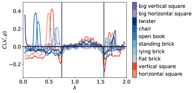
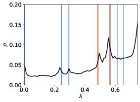
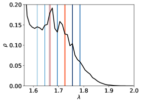
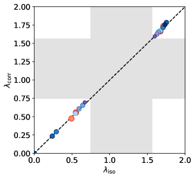
Figure 21: From top to bottom: Correlation between the number of center-vortex objects listed in Tab. 1 and the spectral density, Eq. (39) (first panel); Correlation peaks of the first panel superimposed on the normalized spectral density for the low (second panel) and high modes (third panel); Position of the correlation peaks $\lambda_{\mathrm{corr}}$ against the eigenvalues $\lambda_{\mathrm{iso}}=\{\lambda_{O},\tilde{\lambda}_{O}\}$ of the localized modes found in the presence of isolated objects of the type listed in Tab. 1 (fourth panel). Here $\beta=0.74$, $N_{s}=20$, and $N_{t}=4$.

The simplest center vortices are those of length 4 and 6, depicted in Tab. 1. Diagonalizing gauge configurations that contain one object of type $O$, one obtains a spectrum mostly comprising delocalized modes in the bulk region of the spectrum, and one (possibly degenerate) localized mode $\lambda_{O}$ at the low end of the spectrum, and one, $\tilde{\lambda}_{O}$, at the high end of the spectrum (again possibly degenerate, with the same degeneracy $\mathcal{D}_{O}$ as its low-mode counterpart). The eigenvalues of the localized modes found outside the bulk in these configurations match almost exactly the main peaks and dips in Figs. 1, 2, 3, 13, 14, and 15. We show this by comparing the spectral density of low modes with the position of the localized eigenmodes corresponding to the various objects in Fig. 20. This is no coincidence. In Fig. 21 (first panel) we show the correlation between the number $\mathcal{N}_{O}$ of objects of type $O$ and the spectral density,

$$C(\mathcal{N}_{O},\rho(\lambda))\equiv\frac{\langle\mathcal{N}_{O}\sum_{n}\delta(\lambda-\lambda_{n})\rangle}{\langle\mathcal{N}_{O}\rangle\langle\sum_{n}\delta(\lambda-\lambda_{n})\rangle}-1\,.$$ (39)

Here objects are counted by identifying exact matches between disconnected components of the vortex configuration on the dual lattice and the configurations shown in Tab. 1, possibly rotated or reflected in space, and reflected in the temporal direction. For a given type of object, a strong correlation is found precisely at the position of the corresponding localized low and high eigenmodes, $\lambda_{O}$ and $\tilde{\lambda}_{O}$, found in the presence of a single, isolated object; a clear anticorrelation is also seen near the mobility edges. The position of the peaks in the correlation match almost perfectly those in the spectral density of low modes, as shown in Fig. 21 (second panel), while the matching seems less nice at the high end of the spectrum (Fig. 21, third panel). However, although relatively rare, the objects are not isolated from each other, and so the spectrum is not simply the union of the individual spectra of the configurations corresponding to the objects in Tab. 1, and the positions of the peaks in $\rho$ are expected to deviate from the isolated-object case. On the other hand, a comparison between the positions of the correlation peaks and the eigenvalues of the localized modes for isolated objects (fourth panel) shows that even in a heterogeneous environment the spectrum responds the most to the center-vortex configurations of Tab. 1 almost exactly where the “free” eigenvalue would be. The bigger deviation of the spectral density peaks from the correlation peaks for the high modes is then likely due to the fact that the localized high modes associated with isolated objects have eigenvalues closer to each other than the corresponding localized low modes, and therefore are more likely to mix when several objects are present, distorting the peak structure from the isolated-object case more than at the low end of the spectrum.

It is worth noting that the number of objects of a certain type, divided by the number of its different possible orientations, appears to be distributed according to a Poisson distribution with parameter $\Lambda_{O}=N_{0}Ve^{-k_{O}s}$, where $k_{O}$ is the “order” of the object, i.e., the number of dual lattice plaquettes in the minimal surface having as boundary the closed vortex line that defines the object. At $\beta=0.74$ the numerical coefficients $N_{0}$ and $s$ are $N_{0}=1.82(3)\times 10^{-3}$ and $s=3.17(3)$.

We mention in passing that sharp peaks ending in a cusp were noticed in the spectral density in the deconfined phase in Ref. [19], at $\sqrt{3/2}$ in the physical sector ($\bar{P}>0$), and at $1$ and $\sqrt{2}$ in the unphysical sector ($\bar{P}<0$). These peaks are of an entirely different origin, and are related to the Van Hove singularities of the free spectrum. We discuss this point in Appendix A.

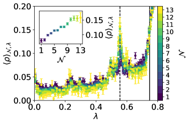
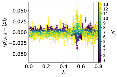
Figure 22: Normalized spectral density at fixed number $\mathcal{N}$ of “vertical squares” (top panel), and its difference with the full normalized spectral density (bottom panel). The dashed line is at $\lambda\simeq 0.55$, which is the eigenvalue of the localized low mode corresponding to an isolated vertical square; the solid line indicates the position of the mobility edge. Here $\beta=0.74$, $N_{s}=20$, and $N_{t}=4$.

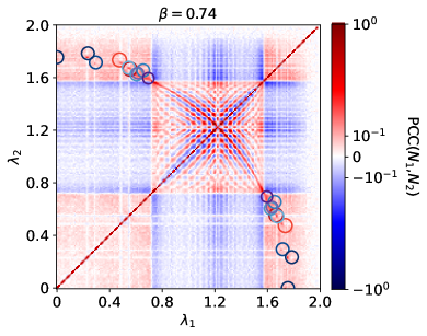
Figure 23: Pearson correlation coefficient for the mode number, Eq. (41). Circles correspond to the pairs of localized low and high modes associated with the objects listed in Tab. 1. Here $\beta=0.74$, $N_{s}=20$, and $N_{t}=4$.

Figure 24: Two-point eigenvector correlator $C$, Eq. (42), in the confined phase at $\beta=0.71$ (top panel) and in the deconfined phase at $\beta=0.74$ (bottom panel). Here $N_{s}=20$ and $N_{t}=4$. For better visualization, a linear scale is used in the range $|C|\leq 10^{-2}$ and a logarithmic scale outside of it.

Further evidence of the relation between the peak structures and the simple center vortex structures is provided by the nearly linear response of the spectral density to the number of objects of type $O$ near $\lambda_{O}$. In Fig. 22 we show the spectral density of low modes obtained using those configurations from one of our ensembles that contain a fixed number of “vertical squares”, for several such numbers. The strongest, and almost linear response is found near $\lambda\simeq 0.55$, which is the eigenvalue of the corresponding localized low mode. For each object type we then counted the number of modes $N_{O}^{(0)}$ within the two peaks of positive correlation seen in Fig. 21, and checked how it related with the number $\mathcal{N}_{O}$ of objects of the given type. We found an approximately linear response, with

$$\left\langle\frac{N_{O}^{(0)}-\langle N_{O}^{(0)}\rangle}{\mathcal{N}_{O}-\langle\mathcal{N}_{O}\rangle}\right\rangle\simeq c\mathcal{D}_{O}\,,$$ (40)

with $\mathcal{D}_{O}$ the degeneracy of the localized modes given in Tab. 1, and $c\simeq 0.79(3)$. The distortive effects on the spectrum due to several objects being present at the same time in a typical gauge configuration are likely the reason of the reduction of $c$ from the naive expectation $c=2$.

Since localized modes originate from the same gauge-field structures, being basically the result of mixing of the localized modes associated with isolated center vortices, an increase in the number of center vortices in the configuration should drive up the number of localized modes independently of where they are found in the spectrum. One then expects a positive correlation in the local density of modes at different points in the localized regime of the spectrum, including between low and high modes. This is clearly visible in Fig. 23, where we show the Pearson correlation coefficient

$$\mathrm{PCC}(N_{1},N_{2})\equiv\frac{\langle(N_{1}-\langle N_{1}\rangle)(N_{2}-\langle N_{2}\rangle)\rangle}{\sqrt{(\langle N_{1}^{2}\rangle-\langle N_{1}\rangle^{2})(\langle N_{2}^{2}\rangle-\langle N_{2}\rangle^{2})}}\,,$$ (41)

between the number of modes $N_{1,2}$ found in disjoint spectral bins of equal size $\Delta\lambda=0.01$. Particularly strong correlations are observed for the pair of bins corresponding to the low and high localized modes associated with one of the simplest objects (i.e., center vortices), $\lambda_{O}$ and $\tilde{\lambda}_{O}$.

One expects to find a similarly strong correlation also between the eigenvectors corresponding to low and high modes near $\lambda_{O}$ and $\tilde{\lambda}_{O}$, as they should be localized in the same region near one of the simplest center-vortex structures. This is confirmed by Fig. 24, where we show the following quantity,

$$C(\lambda_{1},\lambda_{2}) \equiv\frac{\langle\sum_{l_{1}\neq l_{2}}\delta(\lambda_{1}-\lambda_{l_{1}})\delta(\lambda_{2}-\lambda_{l_{2}})X_{l_{1}l_{2}}\rangle}{\left[\Delta(\lambda_{1})\Delta(\lambda_{2})\right]^{\frac{1}{2}}}\,,$$ (42)

$$X_{l_{1}l_{2}} \equiv\left(\textstyle\sum_{n}|\psi_{l_{1}}(n)|^{2}|\psi_{l_{2}}(n)|^{2}\right)-{\textstyle\frac{1}{V}}\,,$$

$$\Delta(\lambda) \equiv\langle\textstyle\sum_{l}\delta(\lambda-\lambda_{l})\left(\mathrm{IPR}_{l}-{\textstyle\frac{1}{V}}\right)\rangle\,.$$

The anticorrelation between localized and bulk modes can be explained by taking into account the sum rule $\sum_{l}|\psi_{l}(n)|^{2}=1$, that follows from the completeness relation for the eigenvectors. In fact, localized modes give large contributions to the sum if $n$ is in the regions where they are localized, i.e., those occupied by center vortices. This leads to almost saturating the sum rule, so that little is left for the delocalized modes to share, leading in practice to them avoiding the vortices.

The positive correlation between localized modes seen in Fig. 24 can be understood as a consequence of the mixing of modes associated with isolated objects, mentioned above. If a configuration contains $N_{O}$ objects of size $V_{O}$, and localized modes typically spread over $n_{O}$ of them, then their typical size is $n_{O}V_{O}$ and the chance that two modes share one and the same object is $(n_{O}/N_{O})^{2}$, and so one finds

$$\sum_{n}|\psi_{l_{1}}(n)|^{2}|\psi_{l_{2}}(n)|^{2} \sim N_{O}V_{O}\left(\frac{n_{O}}{N_{O}}\right)^{2}\left(\frac{1}{n_{O}V_{O}}\right)^{2}$$ (43)

$$=\frac{1}{N_{O}V_{O}}\,,$$

leading to

$$C(\lambda_{1},\lambda_{2})\sim\left(\frac{V}{N_{O}V_{O}}-1\right)[\rho(\lambda_{1})\rho(\lambda_{2})]^{\frac{1}{2}}n_{O}V_{O}\,.$$ (44)

Since $N_{O}V_{O}/V<1$ is the fraction of the lattice occupied by objects, the correlation is positive. As the temperature grows this fraction decreases, and so does the mode size (see Fig. 1), approximated here by $n_{O}V_{O}$, leading therefore to stronger correlations.

Interestingly, in Fig. 24 a positive correlation between low and high modes, particularly strong near $(\lambda_{1},\lambda_{2})=(\lambda_{O},\tilde{\lambda}_{O})$, is observed also in the confined phase. As a nonzero density of finite clusters is present also in the confined phase (see Sec. III.2), it is not surprising that they support the nonzero spectral density of localized high modes, as this result further confirms. It is somewhat surprising, though, that a strong correlation with the spectral regions where the low-mode counterparts would be found survives also in the confined phase, where low modes are delocalized. This indicates that low modes still carry some local structure highly correlated with the center-vortex configuration. This also explain their anticorrelation with the bulk modes.

The quarter-circular structure visible in the bulk in Figs. 23 and 24 reflects the symmetry properties of the free staggered spectrum, Eq. (8). In fact, for $N_{t}$ and $N_{s}$ multiples of 4, there are pairs of free eigenvalues obeying $\lambda(\omega,\vec{p}\,)^{2}+\lambda(\omega^{\prime},\vec{p}^{\,\prime})^{2}=3$, where $\omega^{\prime}-\omega=p_{1}^{\prime}-p_{1}=p_{2}^{\prime}-p_{2}=\frac{\pi}{2}$ corresponding to $k_{0}^{\prime}-k_{0}=k_{1}^{\prime}-k_{1}=k_{2}^{\prime}-k_{2}=\frac{N_{t}}{4}$. The correlation between modes lying on the line $\lambda_{1}^{2}+\lambda_{2}^{2}=3$ remains even in the interacting case, although it is partially smeared out in the confined phase (see Fig. 24, top panel). This can be understood by noticing that if one could neglect the effect of nontrivial plaquettes, then in $d$ spatial dimensions and for generic (compact) gauge group one would find

$$(-iD^{\mathrm{stag}})^{2} \approx\frac{d+1}{2}-\frac{1}{4}\sum_{\mu=1}^{d+1}\left[(U_{\mu}T_{\mu})^{2}+(T_{\mu}^{\dagger}U_{\mu}^{\dagger})^{2}\right]$$ (45)

$$\equiv\frac{d+1}{2}-\tilde{H}\,.$$

Setting $\zeta(n)\equiv i^{\sum_{\mu}n_{\mu}}$, one has $\{\zeta,\tilde{H}\}=0$, meaning that $\tilde{H}$ has a symmetric spectrum, $\tilde{H}\tilde{\psi}_{\pm l}=\pm\tilde{\lambda}_{l}\tilde{\psi}_{\pm l}$, with $\tilde{\lambda}_{l}>0$ and $\tilde{\psi}_{-l}=\zeta\tilde{\psi}_{l}$. One then finds for $(-iD^{\mathrm{stag}})^{2}$ the approximate relations

$$(-iD^{\mathrm{stag}})^{2}\tilde{\psi}_{\pm l}\approx\left(\frac{d+1}{2}\mp\tilde{\lambda}_{l}\right)\tilde{\psi}_{\pm l}\,,$$ (46)

where $\tilde{\psi}_{l}$ and $\tilde{\psi}_{-l}$ have the same local amplitude squared, $\tilde{\psi}_{l}(n)^{\dagger}\tilde{\psi}_{l}(n)=\tilde{\psi}_{-l}(n)^{\dagger}\tilde{\psi}_{-l}(n)$. Since also $[\varepsilon,\tilde{H}]=0$, each eigenvalue is doubly degenerate, and one finds the usual pair of positive and negative eigenvalues of equal magnitude for $-iD^{\mathrm{stag}}$. Consistency with the (anti)periodic boundary conditions requires that $\zeta(n+N_{t}\hat{1})=\zeta(n+N_{s}\hat{\jmath})=\zeta(n)$ for $j=2,\ldots,d+1$, so $i^{N_{t}}=i^{N_{s}}=1$, restricting the validity of this result to the case when $N_{t}$ and $N_{s}$ are both multiples of 4. Negative plaquettes are indeed rare in the deconfined phase, so that the analysis above applies, explaining the strong correlation found in the bulk at $\lambda_{1}^{2}+\lambda_{2}^{2}=3$. In the confined phase negative plaquettes are certainly not rare, but it is reasonable that their effect on the bulk modes partially cancels out, making the explanation above viable.

Although much less well defined, the quarter-circular structure seems to extend also in the (low, high) and (high, low) corners of the plot. Here the argument above certainly does not apply, since it is precisely the nontrivial plaquettes that give rise to localized modes, and so they cannot be neglected. A possible explanation can be obtained combining the sum rule $\sum_{l}\lambda_{l}^{2}|\psi_{l}(n)|^{2}=\frac{d+1}{2}$ (with $d$ again the spatial dimensionality), specific to staggered fermions, with the completeness sum rule $\sum_{l}|\psi_{l}(n)|^{2}=1$ to get $\sum_{l}[\lambda_{l}^{2}-\frac{d+1}{2}]|\psi_{l}(n)|^{2}=0$. If bulk modes in the presence of interactions do not differ much from the free bulk modes, then their total contribution to the sum rule is small, with positive and negative contributions nearly cancelling out. This seems to be the case at least in the deconfined phase, where the argument above shows the existence of pairs of eigenmodes $\psi_{l}$, $\psi^{\prime}_{l}\approx\zeta\psi_{l}$ of $-iD^{\mathrm{stag}}$ with approximately equal local weight, $|\psi^{\prime}_{l}(n)|^{2}\approx|\zeta(n)\psi_{l}(n)|^{2}=|\psi_{l}(n)|^{2}$, and eigenvalues $\lambda_{l}$, $\lambda^{\prime}_{l}$ approximately related as $\lambda_{l}^{2}+\lambda^{\prime\,2}_{l}\approx d+1$. On the other hand, if a localized low mode exists at some $\lambda^{2}<\frac{d+1}{2}$, then a similarly localized high mode should exist near $d+1-\lambda^{2}$ to balance the sum rule.

The results of this Subsection show that the localization of low Dirac modes in the deconfined phase of $\mathbb{Z}_{2}$ is explained by the opening of the spectral pseudogap due to Polyakov loop ordering, and by the presence of disconnected finite clusters, i.e., center vortices not spanning the whole lattice, that are the main localization centers. As both Polyakov loop ordering and the fragmentation of the infinite center cluster are direct manifestations of deconfinement, the strong connection between deconfinement and localization is evident. Notice that center vortices being the main localization centers is not at all in contradiction with the sea/islands picture, as Polyakov loop, islands, and center vortices are very strongly correlated with each other, as shown in the previous Subsection.

IV Conclusions

In this paper we investigated different aspects of the deconfinement transition in finite-temperature 2+1-dimensional $\mathbb{Z}_{2}$ gauge theory on the lattice, and of its relation with the localization of low Dirac modes.

As a first step, we confirmed the presence of an Anderson transition in the spectrum of the staggered Dirac operator, separating localized low-lying modes from delocalized bulk modes. The presence of localized low modes, appearing at the deconfinement transition, was shown in Ref. [19], short only of a finite-size scaling analysis. Here we performed this analysis, fully validating the claims of Ref. [19].

Our results are interesting also from the point of view of disordered systems, independently of their connection with the confinement of quarks. Our finite-size-scaling analysis shows that 2+1-dimensional $\mathbb{Z}_{2}$ gauge theory is another (spatially) two-dimensional disordered system in the orthogonal class displaying a BKT-type Anderson transition [50, 52]. Furthermore, the dependence of the position of the mobility edge on the temperature is rather counterintuitive, and different from what has been observed so far in lattice gauge theories.

We then further established the characterization of the deconfinement transition as a percolation transition of center vortices [39, 40], determining the percolation temperature and finding it in agreement with the deconfinement temperature [34]. An interesting finding is that the critical properties of the vortex percolation transition are different from those of ordinary two-dimensional percolation. This is probably due to the long-range nature of the constraint on the percolating objects, i.e., the requirement that vortices form closed loops on the dual lattice.

We then studied the correlation between center vortices and localized Dirac modes. Not only did we find a strong correlation between the two, but we could also precisely identify the gauge field fluctuations mostly responsible for the localization of both low and high modes, and for the peculiar peak and dip features found in the spectral density and in the mode size.

In 2+1-dimensional $\mathbb{Z}_{2}$ gauge theory the very close connection between confinement and specific topological objects (center vortices, in this case) is almost trivially expected, due to the simplicity of the dynamics (it is nonetheless nice to be able to confirm it explicitly). This allowed us to investigate in an inequivocal way (albeit, perhaps, in too simplified an environment) the connection between deconfinement and localization of Dirac modes, strongly suggested by a wealth of results [1, 2, 3, 4, 5, 6, 7, 8, 9, 10, 11, 12, 13, 14, 15, 16, 17, 18, 19, 20, 21, 22, 23, 24]. Specifically, we looked directly at the correlation between localized modes and the center vortices whose percolation signals confinement. Such a correlation is demonstrated here at the microscopic level, identifying the structures in the gauge configurations mainly responsible for localizing the Dirac modes: these are precisely the most elementary center vortices. The resulting picture is then that as the temperature is lowered and the confinement transition is approached, such vortices approach a percolation transition, and the localized modes they support tend to mix more strongly, therefore tending to delocalize. The connection between the confinement/deconfinement transition and delocalization/localization transition is then fully elucidated in terms of the gauge structures responsible for both. This supports our hope that identifying the structures responsible for low-mode localization in more realistic gauge theories, including the physically relevant case of QCD, can lead to a better understanding of the microscopic mechanism behind confinement.

Appendix A Van Hove singularities

In Ref. [19], sharp peaks ending in a cusp were noticed in the spectral density in the deconfined phase, both in the physical and in the unphysical sector, but no explanation was offered for them. This is provided here.

Due to the ordering of the Polyakov loop, in the deconfined phase the bulk of the spectrum should resemble that of the free theory in the physical sector, and that of the free theory supplemented by a uniform non-trivial Polyakov loop in the unphysical sector. This includes reproducing the Van Hove singularities [58] of the spectral density where the “band energies” $\mathcal{E}_{n}(\vec{p}\,)=\sqrt{(\sin\omega_{n})^{2}+(\sin p_{1})^{2}+(\sin p_{2})^{2}}$ have a vanishing gradient, $\vec{\nabla}\mathcal{E}_{n}(\vec{p}\,)=[2\mathcal{E}_{n}(\vec{p}\,)]^{-1}(\sin 2p_{1},\sin 2p_{2})=0$. Here the various bands are characterized by $\omega_{n}^{\mathrm{phys}}=\frac{(2n+1)\pi}{N_{t}}$ for the physical sector, and $\omega_{n}^{\mathrm{unphys}}=\frac{2n\pi}{N_{t}}$ for the unphysical sector, with $n=0,\ldots,N_{t}-1$ in both cases. The spatial momentum $\vec{p}=(p_{1},p_{2})$ is restricted to the first Brillouin zone; in the large-volume limit, $p_{i}\in[-\pi,\pi]$.

For the $N_{t}=4$ case considered here and in Ref. [19], one has in the physical sector $(\sin\omega_{n}^{\mathrm{phys}})^{2}=1/2$, for $n=0,\ldots,3$, and the gradient vanishes for $p_{1,2}=0,\pm\frac{\pi}{2},\pm\pi$, corresponding to $\mathcal{E}_{n}=\sqrt{1/2},\sqrt{3/2},\sqrt{5/2}$. In the interacting case at $\beta>\beta_{c}$, the smallest and largest values are found in the localized regions of the spectrum , while a Van Hove singularity is indeed seen at $\sqrt{3/2}$. In the unphysical sector one has instead $(\sin\omega_{n}^{\mathrm{unphys}})^{2}=0$, for $n=0,2$, and $(\sin\omega_{n}^{\mathrm{unphys}})^{2}=1$, for $n=1,3$. The gradient again vanishes for $p_{1,2}=0,\pm\frac{\pi}{2},\pm\pi$, corresponding to $\mathcal{E}_{n}=0,1,\sqrt{2},\sqrt{3}$. (More precisely, if $n=0,2$ and all the $p_{i}$ approach $0$ or $\pm\pi$, then $\vec{\nabla}\mathcal{E}_{n}$ tends to zero.) The smallest and largest values are exactly at the edge of the positive spectrum, where deviations from the free behavior are expected and observed in the interacting case; Van Hove singularities are indeed seen at $1$ and $\sqrt{2}$.

References

- García-García and Osborn [2006] A. M. García-García and J. C. Osborn, Nucl. Phys. A770, 141 (2006), arXiv:hep-lat/0512025 [hep-lat] .
- García-García and Osborn [2007] A. M. García-García and J. C. Osborn, Phys. Rev. D 75, 034503 (2007), arXiv:hep-lat/0611019 [hep-lat] .
- Kovács [2010] T. G. Kovács, Phys. Rev. Lett. 104, 031601 (2010), arXiv:0906.5373 [hep-lat] .
- Kovács and Pittler [2010] T. G. Kovács and F. Pittler, Phys. Rev. Lett. 105, 192001 (2010), arXiv:1006.1205 [hep-lat] .
- Bruckmann et al. [2011] F. Bruckmann, T. G. Kovács, and S. Schierenberg, Phys. Rev. D 84, 034505 (2011), arXiv:1105.5336 [hep-lat] .
- Kovács and Pittler [2012] T. G. Kovács and F. Pittler, Phys. Rev. D 86, 114515 (2012), arXiv:1208.3475 [hep-lat] .
- Giordano et al. [2014] M. Giordano, T. G. Kovács, and F. Pittler, Phys. Rev. Lett. 112, 102002 (2014), arXiv:1312.1179 [hep-lat] .
- Nishigaki et al. [2014] S. M. Nishigaki, M. Giordano, T. G. Kovács, and F. Pittler, PoS LATTICE2013, 018 (2014), arXiv:1312.3286 [hep-lat] .
- Ujfalusi et al. [2015] L. Ujfalusi, M. Giordano, F. Pittler, T. G. Kovács, and I. Varga, Phys. Rev. D 92, 094513 (2015), arXiv:1507.02162 [cond-mat.dis-nn] .
- Cossu and Hashimoto [2016] G. Cossu and S. Hashimoto, J. High Energy Phys. 06, 056 (2016), arXiv:1604.00768 [hep-lat] .
- Giordano et al. [2017a] M. Giordano, S. D. Katz, T. G. Kovács, and F. Pittler, J. High Energy Phys. 02, 055 (2017a), arXiv:1611.03284 [hep-lat] .
- Kovács and Vig [2018] T. G. Kovács and R. Á. Vig, Phys. Rev. D 97, 014502 (2018), arXiv:1706.03562 [hep-lat] .
- Holicki et al. [2018] L. Holicki, E.-M. Ilgenfritz, and L. von Smekal, PoS LATTICE2018, 180 (2018), arXiv:1810.01130 [hep-lat] .
- Giordano [2019] M. Giordano, J. High Energy Phys. 05, 204 (2019), arXiv:1903.04983 [hep-lat] .
- Vig and Kovács [2020] R. Á. Vig and T. G. Kovács, Phys. Rev. D 101, 094511 (2020), arXiv:2001.06872 [hep-lat] .
- Bonati et al. [2021] C. Bonati, M. Cardinali, M. D’Elia, M. Giordano, and F. Mazziotti, Phys. Rev. D 103, 034506 (2021), arXiv:2012.13246 [hep-lat] .
- Kovács [2022] T. G. Kovács, PoS LATTICE2021, 238 (2022), arXiv:2112.05454 [hep-lat] .
- Cardinali et al. [2022] M. Cardinali, M. D’Elia, F. Garosi, and M. Giordano, Phys. Rev. D 105, 014506 (2022), arXiv:2110.10029 [hep-lat] .
- Baranka and Giordano [2021] G. Baranka and M. Giordano, Phys. Rev. D 104, 054513 (2021), arXiv:2104.03779 [hep-lat] .
- Baranka and Giordano [2022] G. Baranka and M. Giordano, Phys. Rev. D 106, 094508 (2022), arXiv:2210.00840 [hep-lat] .
- Kehr et al. [2024] R. Kehr, D. Smith, and L. von Smekal, Phys. Rev. D 109, 074512 (2024), arXiv:2304.13617 [hep-lat] .
- Baranka and Giordano [2023] G. Baranka and M. Giordano, Phys. Rev. D 108, 114508 (2023), arXiv:2310.03542 [hep-lat] .
- Bonanno and Giordano [2024] C. Bonanno and M. Giordano, Phys. Rev. D 109, 054510 (2024), arXiv:2312.02857 [hep-lat] .
- Giordano and Kovács [2021] M. Giordano and T. G. Kovács, Universe 7, 194 (2021), arXiv:2104.14388 [hep-lat] .
- Anderson [1958] P. W. Anderson, Phys. Rev. 109, 1492 (1958).
- Thouless [1974] D. J. Thouless, Phys. Rep. 13, 93 (1974).
- Lee and Ramakrishnan [1985] P. A. Lee and T. V. Ramakrishnan, Rev. Mod. Phys. 57, 287 (1985).
- Kramer and MacKinnon [1993] B. Kramer and A. MacKinnon, Rep. Prog. Phys. 56, 1469 (1993).
- Evers and Mirlin [2008] F. Evers and A. D. Mirlin, Rev. Mod. Phys. 80, 1355 (2008), arXiv:0707.4378 [cond-mat.mes-hall] .
- Giordano et al. [2015] M. Giordano, T. G. Kovács, and F. Pittler, J. High Energy Phys. 04, 112 (2015), arXiv:1502.02532 [hep-lat] .
- Giordano et al. [2016] M. Giordano, T. G. Kovács, and F. Pittler, J. High Energy Phys. 06, 007 (2016), arXiv:1603.09548 [hep-lat] .
- Giordano et al. [2017b] M. Giordano, T. G. Kovács, and F. Pittler, Phys. Rev. D 95, 074503 (2017b), arXiv:1612.05059 [hep-lat] .
- Wipf [2013] A. Wipf, Statistical approach to quantum field theory: An introduction, Vol. 864 (Springer-Verlag, Berlin Heidelberg, 2013).
- Caselle and Hasenbusch [1996] M. Caselle and M. Hasenbusch, Nucl. Phys. B 470, 435 (1996), arXiv:hep-lat/9511015 .
- von Smekal [2012] L. von Smekal, Nucl. Phys. B Proc. Suppl. 228, 179 (2012), arXiv:1205.4205 [hep-ph] .
- Swendsen and Wang [1987] R. H. Swendsen and J.-S. Wang, Phys. Rev. Lett. 58, 86 (1987).
- Wolff [1989] U. Wolff, Phys. Rev. Lett. 62, 361 (1989).
- Biddle et al. [2023] J. C. Biddle, W. Kamleh, and D. B. Leinweber, Phys. Rev. D 107, 094507 (2023), arXiv:2302.05897 [hep-lat] .
- Engelhardt et al. [2000] M. Engelhardt, K. Langfeld, H. Reinhardt, and O. Tennert, Phys. Rev. D 61, 054504 (2000), arXiv:hep-lat/9904004 .
- Gliozzi et al. [2002] F. Gliozzi, M. Panero, and P. Provero, Phys. Rev. D 66, 017501 (2002), arXiv:hep-lat/0204030 .
- Altshuler and Shklovskii [1986] B. L. Altshuler and B. I. Shklovskii, Sov. Phys. JETP 64, 127 (1986).
- Mehta [2004] M. L. Mehta, Random matrices, 3rd ed., Pure and Applied Mathematics, Vol. 142 (Academic Press, 2004).
- Verbaarschot and Wettig [2000] J. J. M. Verbaarschot and T. Wettig, Ann. Rev. Nucl. Part. Sci. 50, 343 (2000), arXiv:hep-ph/0003017 [hep-ph] .
- Shklovskii et al. [1993] B. I. Shklovskii, B. Shapiro, B. R. Sears, P. Lambrianides, and H. B. Shore, Phys. Rev. B 47, 11487 (1993).
- Brody [1973] T. A. Brody, Lett. Nuovo Cimento 7, 482 (1973).
- Scaramazza et al. [2016] J. A. Scaramazza, B. S. Shastry, and E. A. Yuzbashyan, Phys. Rev. E 94, 032106 (2016), arXiv:1604.01691 [cond-mat.mes-hall] .
- Kalmeyer et al. [1993] V. Kalmeyer, D. Wei, D. P. Arovas, and S. Zhang, Phys. Rev. B 48, 11095 (1993).
- Zhang and Arovas [1994] S.-C. Zhang and D. P. Arovas, Phys. Rev. Lett. 72, 1886 (1994), arXiv:cond-mat/9312010 [cond-mat] .
- Liu et al. [1999a] W.-S. Liu, Y. Chen, S.-J. Xiong, and D. Y. Xing, Phys. Rev. B 60, 5295 (1999a).
- Liu et al. [1999b] W.-S. Liu, T. Chen, and S.-J. Xiong, J. Phys. Condens. Matter 11, 6883 (1999b).
- Xie et al. [1998] X. C. Xie, X. R. Wang, and D. Z. Liu, Phys. Rev. Lett. 80, 3563 (1998).
- Zhang et al. [2009] Y.-Y. Zhang, J. Hu, B. A. Bernevig, X. R. Wang, X. C. Xie, and W. M. Liu, Phys. Rev. Lett. 102, 106401 (2009), arXiv:0810.1996 .
- Lehoucq et al. [1998] R. B. Lehoucq, D. C. Sorensen, and C. Yang, ARPACK users’ guide: solution of large-scale eigenvalue problems with implicitly restarted Arnoldi methods (SIAM, 1998).
- Lepage et al. [2002] G. P. Lepage, B. Clark, C. T. H. Davies, K. Hornbostel, P. B. Mackenzie, C. Morningstar, and H. Trottier, Nucl. Phys. B Proc. Suppl. 106, 12 (2002), arXiv:hep-lat/0110175 .
- James and Roos [1975] F. James and M. Roos, Comput. Phys. Commun. 10, 343 (1975).
- Stauffer and Aharony [1992] D. Stauffer and A. Aharony, Introduction To Percolation Theory: Second Edition (Taylor & Francis, London, 1992).
- Anderson et al. [1999] E. Anderson, Z. Bai, C. Bischof, S. Blackford, J. Demmel, J. Dongarra, J. Du Croz, A. Greenbaum, S. Hammarling, A. McKenney, and D. Sorensen, LAPACK Users’ Guide (SIAM, Philadelphia, 1999).
- Ashcroft and Mermin [1976] N. W. Ashcroft and N. D. Mermin, Solid State Physics (Saunders College Publishing, Philadelphia, 1976).