Sketched Lanczos of Fisher matrix for scaling up Uncertainty Estimation

Sketched matrix free of Fisher matrix for scaling up Uncertainty Estimation

Sketching Fisher matrix for scaling up Uncertainty Estimation

Abstract

In order to safely deploy Deep Neural Networks (DNNs) in mission-critical applications, we must be able to measure their prediction uncertainty fast and reliably. To this end, we develop Sketched Lanczos Score: an architecture-agnostic uncertainty score that can be applied to pre-trained DNNs with minimal overhead. We combine Lanczos algorithm with dimensionality reduction techniques to compute a sketch of the leading eigenvectors of the Fisher information matrix, or ggn. Empirically, we evaluate our score in the low-memory regime across a multitude of tasks and show that Sketched Lanczos Score yields well-calibrated uncertainties, reliably detects out-of-distribution examples, and consistently outperfoms existing methods. $Mio$: explain better memory thing

1 Introduction

The best-performing uncertainty quantification methods share the same problem: scaling. Practically this prevents their use for deep neural networks with high parameter counts. Perhaps, the simplest way of defining such a score is to independently train several models, perform inference, and check how consistent predictions are across models. The overhead of the resulting ’Deep Ensemble’ (Lakshminarayanan et al., 2017) notably introduces a multiplicative overhead equal to the ensemble size. Current approaches aim to reduce the growth in training time costs by quantifying uncertainty through local information of a single pre-trained model. This approach has shown some success for methods like Laplace’s approximation (MacKay, 1992; Immer et al., 2021; Khan et al., 2019), swag (Maddox et al., 2019), scod (Sharma et al., 2021) or Local Ensembles (Madras et al., 2019). They avoid the need to re-train but still have impractical memory needs.

A popular approach to characterizing local information is the empirical Fisher information matrix, which essentially coincides with the Generalized Gauss-Newton (ggn) matrix (Kunstner et al., 2019). Unfortunately, for a $p$-parameter model, the ggn is a $p\times p$ matrix, yielding such high memory costs that it cannot be instantiated for anything but the simplest models. The ggn is, thus, mostly explored through approximations, e.g. block-diagonal (Botev et al., 2017), Kronecker-factorized (Ritter et al., 2018a; Lee et al., 2020; Martens & Grosse, 2015) or even diagonal (Ritter et al., 2018b; miani2022laplacian). An alternative heuristic is to only assign uncertainties to a subset of the model parameters (Daxberger et al., 2021b; Kristiadi et al., 2020), e.g. the last layer.

Instead, we approximate the ggn with a low-rank matrix. A rank-$k$ approximation of the ggn can be computed using Lanczos algorithm (Madras et al., 2019; Daxberger et al., 2021a) or truncated singular value decomposition (svd) (Sharma et al., 2021). These approaches deliver promising uncertainty scores but are limited by their memory footprint. Indeed all aforementioned techniques require $k\cdot p$ memory. Models with high parameter counts are, thus, reduced to only being able to consider very small approximate ranks.

In this work, we design a novel algorithm to compute the local ensemble uncertainty estimation score introduced by Madras et al. (2019), reintroduced in Section 2.1. Our algorithm is substantially more memory-efficient than the previous one both in theory and practice, thus circumventing the main bottleneck of vanilla Lanczos and randomized svd (Figure 1). To that end, we employ sketching dimensionality-reduction techniques, reintroduced in Section 2.3, that trade a small-with-high-probability error in some matrix-vector operations for a lower memory usage. Combining the latter with the Lanczos algorithm (reintroduced in Section 2.2) results in the novel Sketched Lanczos Score.
This essentially drops the memory consumption from $\mathcal{O}(pk)$ to $\mathcal{O}(k^{2}\varepsilon^{-2})$ in exchange for a provably bounded error $\varepsilon$, independently on the number of parameters $p$ (up to log-terms).

Applying this algorithm in the deep neural networks settings allows us to scale up the approach from Madras et al. (2019) and obtain a better uncertainty score for a fixed memory budget.

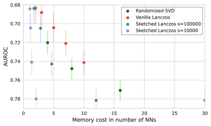
Figure 1: OoD detection performance ($\swarrow$) on a ResNet.

Our contribution is twofold: (1) we prove that orthogonalization approximately commutes with sketching in Section 3, which makes it possible to sketch Lanczos vectors on the fly and orthogonalize them post-hoc, with significant memory savings; (2) we empirically show that, in the low-memory-budget regime, the disadvantage of introducing noise through sketching is outweighed by a higher-rank approximation, thus performing better than baselines when the same amount of memory is used.

2 Background

Let $f_{\theta}:\mathbb{R}^{d}\rightarrow\mathbb{R}^{t}$ denote a neural network with parameter $\theta\in\mathbb{R}^{p}$, or equivalently $f:\mathbb{R}^{p}\times\mathbb{R}^{d}\rightarrow\mathbb{R}^{t}$. Let $\mathbf{J}_{\theta^{\prime}}(x)=\nabla_{\theta}f_{\theta}(x)|_{\theta=\theta^{\prime}}\in\mathbb{R}^{t\times p}$ be its Jacobian with respect to the parameters, evaluated at a datapoint $x\in\mathbb{R}^{d}$. Given a training dataset $\mathcal{D}=\{(x_{i},y_{i})\}_{i=1,\dots,n}$ and a loss function $\mathcal{L}(\theta)=\sum_{(x,y)\in\mathcal{D}}\ell(y,f(x,\theta)$, the Generalized Gauss-Newton matrix (ggn) is defined as

$$\mathbf{G}_{\theta}=\sum_{i=1}^{n}\mathbf{J}_{\theta}(x_{i})^{\top}\mathbf{H}(x_{i})\mathbf{J}_{\theta}(x_{i}),$$ (1)

where $\mathbf{H}(x_{i})=\nabla^{2}_{f_{\theta}(x_{i})}\ell(y_{i}|f_{\theta}(x_{i}))\in\mathbb{R}^{t\times t}$ is the Hessian of the loss with respect to the neural network output. We reduce the notational load by stacking the per-datum Jacobians into $\mathbf{J}_{\theta}=[\mathbf{J}_{\theta}(x_{1});\ldots;\mathbf{J}_{\theta}(x_{n})]\in\mathbb{R}^{nt\times p}$ and similarly for the Hessians, and write the ggn matrix as $\mathbf{G}_{\theta}=\mathbf{J}_{\theta}^{\top}\mathbf{H}\mathbf{J}_{\theta}$. For extended derivations and connections with the Fisher matrix we refer to the excellent review by Kunstner et al. (2019). In the following, we assume access to a pre-trained model with parameter $\theta^{*}$ and omit the dependency of $\mathbf{G}$ on $\theta^{*}$.

Computationally we emphasize that Jacobian-vector products can be performed efficiently when $f$ is a deep nn. Consequently, the ggn-vector product has twice the cost of a gradient backpropagation, at least for common choices of $\ell$ like mse or cross-entropy (khan2021bayesian).

2.1 Uncertainty score

We measure the uncertainty at a datapoint $x$ as the variance of the prediction $f_{\theta}(x)$ with respect to a distribution over parameter $\theta$ defined at training time and independently of $x$. This general scheme has received significant attention. For example, Deep Ensemble (Lakshminarayanan et al., 2017) uses a sum of delta distribution supported on independently trained models, while methods that only train a single network $\theta^{*}$ generally use a Gaussian $\mathcal{N}(\theta|\theta^{*},M)$ with covariance $M\in\mathbb{R}^{p\times p}$. In the latter case, a first-order approximation of the prediction variance is given by a $M$-norm of the Jacobian

$$\textsc{Var}_{\theta\sim\mathcal{N}(\theta|\theta^{*},M)}[f_{\theta}(x)]\approx\textsc{Var}_{\theta\sim\mathcal{N}(\theta|\theta^{*},M)}\left[f^{L}_{\theta}(x)\right]=\textsc{Tr}(\mathbf{J}_{\theta^{*}}(x)\cdot M\cdot\mathbf{J}_{\theta^{*}}(x)^{\top}),$$ (2)

where $f^{L}_{\theta}(x)=f_{\theta}(x)+\mathbf{J}_{\theta^{*}}(x)\cdot(\theta^{*}-\theta)$ is a linearization of $\theta\mapsto f_{\theta}(x)$ around $\theta^{*}$.

The ggn matrix (or empirical Fisher; Kunstner et al. (2019)) is notably connected to uncertainty measures and, more specifically, to the choice of the matrix $M$. Different theoretical reasoning leads to different choices and we focus on two of them:

$$\Meig=(\mathbf{G}+\alpha\mathbb{I}_{p})^{-1}\qquad\qquad\Mnoeig=\mathbb{I}-\Pi_{\mathbf{G}},$$ (3)

where $\Pi_{\mathbf{G}}$ is the projection onto the non-zero eigenvectors of $\mathbf{G}$ and $\alpha>0$ is a constant.

Madras et al. (2019) justify $\Mnoeig$ through small perturbation along zero-curvature directions. Immer et al. (2021) justify $\Meig$ in the Bayesian setting where $\alpha$ is interpreted as prior precision. We do not question these score derivations and refer to the original works, but we highlight their similarity. Given an orthonormal eigen-decomposition of $\mathbf{G}=\sum_{i}\lambda_{i}v_{i}v_{i}^{\top}$ we see that

$$\Meig=\sum_{i}\frac{1}{\lambda_{i}+\alpha}v_{i}v_{i}^{\top}\qquad\Mnoeig=\sum_{i}\delta_{\{\lambda_{i}=0\}}v_{i}v_{i}^{\top}.$$ (4)

Thus both covariances are higher in the directions of zero-eigenvalues, and the hyperparameter $\alpha$ controls how many eigenvectors are relevant in $\Meig$.

Practical choices. The matrix $\mathbf{G}$ is too big to even be stored in memory and approximations are required, commonly in a way that allows access to either the inverse or the projection. A variety of techniques are introduced like diagonal, block diagonal, and block kfac which also allow for easy access to the inverse. Another line of work, like swag (Maddox et al., 2019), directly tries to find an approximation of the covariance $M$ based on stochastic gradient descent trajectories.

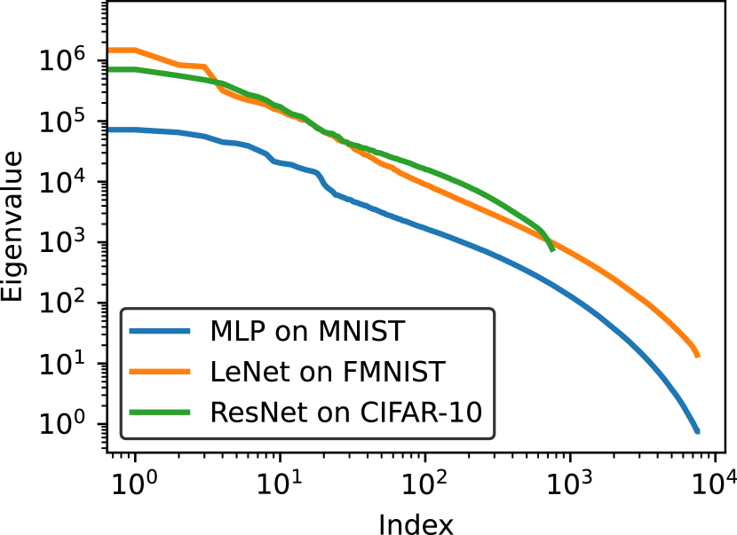
Figure 2: ggn eigenvalues exponential decay. Average and standard deviation over 5 seeds. Details are in Figure 11.

Alternatively, low-rank approximations use the eigen-decomposition relative to the top $k$ eigenvalues, which allows direct access to both inverse and projection.

Is low-rank a good idea? The spectrum of the ggn has been empirically shown to decay exponentially (Sagun et al., 2017; Papyan, 2018; Ghorbani et al., 2019) (see Figure 2). We investigate this phenomenon further in Figure 11 with an ablation over Lanczos hyperparameters. This fast decay implies that the quality of a rank-$k$ approximation of $\mathbf{G}$ improves exponentially w.r.t. $k$ if we measure it with an operator or Frobenius norm, thus supporting the choice of low-rank approximation. Moreover, in the overparametrized setting $p\gg nt$, the rank of the ggn is by construction at most $nt$, which is closely linked with functional reparametrizations (roy2024reparameterization).

The low-rank approach has been applied intensively (Madras et al., 2019; Daxberger et al., 2021a; Sharma et al., 2021) with success, although always limited by memory footprint of $pk$. Madras et al. (2019) argue in favor of a not-too-high $k$ also from a numerical perspective, as using the “small” eigenvectors appears sensitive to noise and consequently is not robust.

2.2 The Lanczos algorithm

The Lanczos algorithm is an iterative method for tridiagonalizing a symmetric matrix $G$. If stopped at iteration $k$, Lanczos returns a column-orthonormal matrix $V=[V_{1}|\dots|V_{k}]\in\mathbb{R}^{p\times k}$ and a tridiagonal matrix $T\in\mathbb{R}^{k\times k}$ such that $V^{\top}GV=T$. The range space of $V$ corresponds to the Krylov subspace $\mathcal{K}_{k}=\texttt{span}\{v,Gv,\dots,G^{k-1}v\}$, where $v=V_{1}$ is a randomly chosen vector. Provably, $\mathcal{K}_{k}$ approximates the eigenspace spanned by the top-$k$ eigenvectors of $G$, i.e. those corresponding to the eigenvalues of largest values (Meurant, 2006). Thus, $VTV^{\top}$ approximates the projection of $G$ onto its top-$k$ eigenspace. Notice that projecting $G$ onto its top-$k$ eigenspace yields the best rank-$k$ approximation of $G$ under any unitarily-invariant norm (Mirsky, 1960). Once the decomposition $G\approx VTV^{\top}$ is available, we can retrieve an approximation to the top-$k$ eigenpairs of $G$ by diagonalizing $T$ into $T=W\Lambda W^{\top}$​​, which can be done efficiently for tridiagonal matrices (Dhillon, 1997). It has both practically and theoretically been found that this eigenpairs’ approximation is very good. We point the reader to Meurant (2006) and Cullum & Willoughby (2002) for a comprehensive survey on this topic.

The benefits of Lanczos.

Lanczos has two features that make it particularly appealing. First, Lanczos does not need explicit access to the input matrix $G$, but only access to an implementation of $G$-vector product $u\mapsto Gu$. Second, Lanczos uses a small working space: only $3p$ floating point numbers, where the input matrix is $p\times p$. Indeed, we can think of Lanczos as releasing its output in streaming and only storing a small state consisting of the last three vectors $V_{i-1},V_{i}$ and $V_{i+1}$.

The downsides of Lanczos.

Unfortunately, the implementation of Lanczos described above is prone to numerical instability, causing $V_{1}\dots V_{k}$ to be far from orthogonal. A careful analysis of the rounding errors causing this pathology was carried out by Paige (1971, 1976, 1980). To counteract, a standard technique is to re-orthogonalize $V_{i+1}$ against all $\{V_{j}\}_{j\leq i}$, at each iteration. This technique has been employed to compute the low-rank approximation of huge sparse matrices (Simon & Zha, 2000), as well as by Madras et al. (2019) to compute an approximation to the top-$k$ eigenvectors. Unfortunately, this version of Lanczos loses one of the two benefits described above, in that it must store a larger state consisting of the entire matrix $V$. Therefore, we dub this version of the algorithm hi-memory Lanczos and the memory-efficient version described above low-memory Lanczos. See Appendix B for a comprehensive discussion on these two versions.

Post-hoc orthogonalization Lanczos.

Alternatively, instead of re-orthogonalizing at every step as in hi-memory Lanczos , we can run low-memory Lanczos , store all the vectors, and orthogonalize all together at the end. Based on the observations of Paige (1980), we expect that orthogonalizing the output of low-memory Lanczos post-hoc should yield an orthonormal basis that approximately spans the top-$k$ eigenspace, similar to hi-memory Lanczos . This post-hoc version of Lanczos is however insufficient. It avoids the cost of orthogonalizing at every iteration but still requires storing the vectors, thus losing again the benefit of memory requirement. Or at least it does unless we find an efficient way to store the vectors.

2.3 Sketching

Sketching is a key technique in randomized numerical linear algebra (Martinsson & Tropp, 2020) to reduce memory requirements. Specifically, sketching embeds high dimensional vectors from $\mathbb{R}^{p}$ into a lower-dimensional space $\mathbb{R}^{s}$, such that the expected norm error of vector dot-products is bounded, and, as a result, also the score in Equation 2. Here we give a concise introduction to this technique.

Definition 2.1 (Subspace embedding).

Fix $\varepsilon>0$. A $(1\pm\varepsilon)$ $\ell_{2}$-subspace embedding for the column space of an $p\times k$ matrix $U$ is a matrix $S$ for which for all $y\in\mathbb{R}^{k}$

$$\lVert SUy\rVert_{2}=(1\pm\varepsilon)\lVert Uy\rVert_{2}.$$ (5)

	Time	Memory
Dense JL	$\mathcal{O}(p^{\omega})$	$p^{2}$
Sparse JL	$\mathcal{O}(p\cdot\varepsilon s)$	$p\cdot\varepsilon s$
srft	$\mathcal{O}(p\log p)$	$p+s$

Table 1: Sketch complexities comparison. Here $\omega$ is such that the current best matrix-multiplication algorithm runs in time $n^{\omega}$.

The goal is to design an oblivious subspace embedding, that is a random matrix $S$ such that, for any matrix $U$, $S$ is a subspace embedding for $U$ with sufficiently high probability. In our method, we use a Subsampled Randomized Fourier Transform (srft) to achieve this goal (Ailon & Chazelle, 2009). A srft is a $s\times p$ matrix defined by the product $\nicefrac{{1}}{{\sqrt{sp}}}PHD$, where $D$ is a diagonal matrix where each diagonal entry is an independent Rademacher random variable, $H$ is the discrete Fourier transform, and $P$ is a diagonal matrix where $s$ random diagonal entries are set to one and every other entry is set to zero. Thanks to the Fast Fourier Transform algorithm, srft can be evaluated in $O(p\log p)$ time, and its memory footprint is only $p+s$.

The following theorem shows that, as long as the sketch size $s$ is big enough, srft is an oblivious subspace embedding with high probability.

Theorem 2.2 (Essentially, Theorem 7 in Woodruff et al. (2014)).

For any $p\times k$ matrix $U$, srft is a $(1\pm\varepsilon)$-subspace embedding for the column space of $U$ with probability $1-\delta$ as long as $s=\Omega((k+\log p)\varepsilon^{-2}\log(k/\delta))$.

We stress that, although several other random projections work as subspace embeddings, our choice is not incidental. Indeed other sketches, including the Sparse JL transform (Kane & Nelson, 2014; Nelson & Nguyên, 2013) or the Dense JL transform (Theorem 4, Woodruff et al. (2014)), theoretically have a larger memory footprint or a worse trade-off between $s$ and $k$, as clarified in Table 1. From such a comparison, it is clear that srft is best if our goal is to minimize memory footprint. At the same time, evaluation time is still quasilinear.

3 Method

We now develop the novel Sketched Lanczos algorithm by combining the ‘vanilla’ Lanczos algorithm (Section 2.2) with sketching (Section 2.3). Pseudo-code is presented in Algorithm 1. Next, we apply this algorithm in the uncertainty quantification setting and compute an approximation of the score in Equation 2 due to Madras et al. (2019). Our motivation is that given a fixed memory budget, the much lower memory footprint induced by sketching allows for a higher-rank approximation of $\mathbf{G}$.

3.1 Sketched Lanczos

We find the best way to explain our algorithm is to first explain a didactic variant of it, where sketching and orthogonalization happen in reverse order.

Running low-memory Lanczos for $k$ iterations on a $p\times p$ matrix iteratively constructs the columns of a $p\times k$ matrix $V$. Then, post-hoc, we re-orthogonalize the columns of $V$ in a matrix $U\in\mathbb{R}^{p\times k}$. Such a matrix is expensive to store due to the value of $p$, but if we sample a srft sketch matrix $S\in\mathbb{R}^{s\times p}$, we can then store a sketched version $SU\in\mathbb{R}^{s\times k}$, saving memory as long as $s<p$. In other words, this is post-hoc orthogonalization Lanczos with a sketching at the end.

We observe that sketching the columns of $U$ is sufficient to $\varepsilon$-preserve the norm of matrix-vector products, with high probability. In particular, the following lemma holds (proof in Appendix A).

Lemma 3.1 (Sketching low-rank matrices).

Fix $0<\varepsilon,\delta<\sfrac{1}{2}$ and sample a random $s\times p$ srft matrix $S$. Then, for any $v\in\mathbb{R}^{p}$ and any matrix $U\in\mathbb{R}^{p\times k}$ with $||v||_{2},||U||_{2}=\mathcal{O}(1)$ we have

$$\Pr_{S}\!\Big{(}{\lVert(SU)^{\top}(Sv)\rVert_{2}=\lVert U^{\top}v\rVert_{2}\pm\varepsilon}\Big{)}>1-\delta.$$ (6)

as long as $s=\Omega(k\varepsilon^{-2}\cdot\log p\cdot\log(k/\delta))$.

This algorithm may initially seem appealing since we can compute a tight approximation of $\|U^{\top}v\|$ by paying only $s\times k$ in memory (plus the neglectable cost of storing $S$). However, as an intermediate step of such an algorithm, we still need to construct the matrix $U$, paying $p\times k$ in memory. Indeed, we defined $U$ as a matrix whose columns are an orthonormal basis of the column space of $V$ and we would like to avoid storing $V$ explicitly and rather sketch each column $V_{i}$ on the fly, without ever paying $p\times k$ memory. This requires swapping the order of orthogonalization and sketching.

This motivates us to prove that if we orthonormalize the columns of $SV$ and apply the same orthonormalization steps to the columns of $V$, then we obtain an approximately orthonormal basis. Essentially, this means that sketching and orthogonalization approximately commute. As a consequence, we can use a matrix whose columns are an orthonormal basis of the column space of $SV$ as a proxy for $SU$ while incurring a small error. Formally, the following holds (proof in Appendix A).

Lemma 3.2 (Orthogonalizing the sketch).

Fix $0<\varepsilon,\delta<\sfrac{1}{2}$ and sample a random $s\times p$ srft matrix $S$. As long as $s=\Omega(k\varepsilon^{-2}\cdot\log p\cdot\log(k/\delta))$ the following holds with probability $1-\delta$.

Given any $p\times k$ full-rank matrix $V$, decompose $V=UR$ and $SV=U_{S}R_{S}$ so that $U\in\mathbb{R}^{p\times k}$, $U_{S}\in\mathbb{R}^{s\times k}$ and both $U$ and $U_{S}$ have orthonormal columns. For any unit-norm $v\in\mathbb{R}^{p}$ we have

$$\lVert U_{S}^{\top}(Sv)\rVert_{2}=\lVert U^{\top}v\rVert_{2}\pm\varepsilon.$$ (7)

In Lemma 3.1, we proved that given a matrix $U$ with orthonormal columns we can store $SU$ instead of $U$ to compute $v\mapsto||U^{\top}v||_{2}$ while incurring a small error. However, in our use case, we do not have explicit access to $U$. Indeed, we abstractly define $U$ as a matrix whose columns are an orthonormal basis of the column space of $V$, but we only compute $U_{S}$ as a matrix whose columns are an orthonormal basis of the column space of $SV$, without ever paying $p\cdot k$ memory. Lemma 3.2 implies that the resulting error is controlled.

Algorithm 1 lists the pseudocode of our new algorithm: Sketched Lanczos Score.

Algorithm 1 Sketched Lanczos Score

1:  Input: Rank $k$, sketch matrix $S\mathbb{\in}\mathbb{R}^{s\times p}$, matrix-vector product function $v\mapsto Gv$ for $G\mathbb{\in}\mathbb{R}^{p\times p}$.

2:  Initialize $v_{0}\in\mathbb{R}^{p}$ as a uniformly random unit-norm vector.

3:  for $i$ in $1,\ldots k$ do

4:     $v_{i}\leftarrow\textsc{LanczosIteration}(v_{i-1},v\mapsto Gv)$      (glossing over the tridiagonal detail)

5:     Sketch and store $v^{S}_{i}\leftarrow Sv_{i}$

6:  end for

7:  Construct the matrix $V_{S}=[v^{S}_{1},\ldots,v^{S}_{k}]\in\mathbb{R}^{s\times k}$

8:  Orthogonalize the columns of $V_{S}$ and return $U_{S}\in\mathbb{R}^{s\times k}$

Preconditioned Sketched Lanczos. We empirically noticed that low-memory Lanczos ’ stability is quite dependent on the conditioning number of the considered matrix. From this observation, we propose a slight modification of Sketched Lanczos that trades some memory consumption for numerical stability.

The idea is simple, we first run hi-memory Lanczos for $k_{0}$ iterations, obtaining an approximation of the top-$k_{0}$ eigenspectrum $U_{0}\in\mathbb{R}^{p\times k_{0}},\Lambda_{0}\in\mathbb{R}^{k_{0}\times k_{0}}$. Then we define a new matrix-vector product

$$\bar{\mathbf{G}}v=(\mathbf{G}-U_{0}\Lambda_{0}U_{0}^{\top})v$$ (8)

and run Sketched Lanczos for $k_{1}$ iterations on this new, better-conditioned, matrix $\bar{\mathbf{G}}$. This results in a $U_{S}\in\mathbb{R}^{s\times k_{1}}$ with sketched orthogonal columns. With $k=k_{1}+k_{0}$, the simple concatenation $[SU_{0}|U_{S}]\in\mathbb{R}^{(k_{0}+k_{1})\times s}$ is a sketched orthogonal $k$-dimensional base of the top-$k$ eigenspace of $\mathbf{G}$, analogous to non-preconditioned Sketched Lanczos. The extra stability comes at a memory cost of $k_{0}\cdot p$, thus preventing $k_{0}$ from being too large.

3.2 Sketched Lanczos Uncertainty score (slu)

The uncertainty score in Equation 2 is computed by first approximating the Generalized Gauss-Newton matrix $\mathbf{G}$. The approach of constructing an orthonormal basis $U\in\mathbb{R}^{p\times k}$ of the top-$k$ eigenvectors of $\mathbf{G}$ with relative eigenvalues $\Lambda$, leads to the low-rank approximation $\mathbf{G}\approx U\Lambda U^{\top}$. This step is done, for example, by Madras et al. (2019) through hi-memory Lanczos and by Sharma et al. (2021) through truncated randomized svd. In this step, we employ our novel Sketched Lanczos. Similar to Madras et al. (2019), we focus on the score with $\Mnoeig$ and thus we neglect the eigenvalues.

Having access to $U$, we can compute the score for a test datapoint $x\in\mathbb{R}^{d}$ as

$$\textsc{Var}[f_{\theta}(x)]\approx\textsc{Tr}\left(\mathbf{J}_{\theta^{*}}(q)\cdot(\mathbb{I}-UU^{\top})\cdot\mathbf{J}_{\theta^{*}}(q)^{\top}\right)=\lVert\mathbf{J}_{\theta^{*}}(q)\rVert^{2}_{F}-\lVert\mathbf{J}_{\theta^{*}}(q)U\rVert^{2}_{F},$$ (9)

which clarifies that computing $||\mathbf{J}_{\theta^{*}}(q)U||_{F}$ is the challenging bit to retrieve the score in Equation 2. Note that $\lVert\mathbf{J}_{\theta^{*}}(q)\rVert^{2}_{F}$ can be computed exactly with $t$ Jacobian-vector products.

Computing the uncertainty score through sketching.

Employing the novel Sketched Lanczos algorithm we can $\varepsilon$-approximate the score in Equation 9, with only minor modifications. Running the algorithm for $k$ iterations returns a matrix $U_{S}\in\mathbb{R}^{s\times k}$, which we recall is the orthogonalization of $SV$ where $V\in\mathbb{R}^{p\times k}$ are the column vectors iteratively computed by Lanczos.

Having access to $U_{S}$, we can then compute the score for a test datapoint $x\in\mathbb{R}^{d}$ as

$$\textsc{slu}(x)=\lVert\mathbf{J}_{\theta^{*}}(q)\rVert^{2}_{F}-\lVert U_{S}^{\top}\left(S\mathbf{J}_{\theta^{*}}(q)^{\top}\right)\rVert^{2}_{F}$$ (10)

where parentheses indicate the order in which computations should be performed: first a sketch of $\mathbf{J}_{\theta^{*}}(q)$ is computed, and then it is multiplied by $U_{S}^{\top}$. Algorithm 2 summarizes the pipeline.

Algorithm 2 Sketched Lanczos Uncertainty score (slu)

1:  Input: Observed data $\mathcal{D}$, trained map parameter $\theta^{*}\in\mathbb{R}^{p}$, approximation rank $k$, sketch size $s$.

2:  Initialize srft sketch matrix $S\mathbb{\in}\mathbb{R}^{s\times p}$

3:  Initialize ggn-vector product $v\mapsto\mathbf{G}v=\sum_{x_{i}\in\mathcal{D}}\mathbf{J}_{\theta^{*}}(x_{i})^{\top}\mathbf{H}(x_{i})\mathbf{J}_{\theta^{*}}(x_{i})v$

4:  $U_{S}\leftarrow\textsc{Sketched Lanczos}(k,S,v\mapsto\mathbf{G}v)$

5:  At query time, for a test point $x$ return $\lVert\mathbf{J}_{\theta^{*}}(x)\rVert^{2}_{F}-\lVert U_{S}^{\top}(S\mathbf{J}_{\theta^{*}}(x)^{\top})\rVert^{2}_{F}$

Approximation quality.

Recall that the Jacobian $\mathbf{J}_{\theta^{*}}(q)$ is a $t\times p$ matrix, where $t$ is the output size of the neural network. A slight extension of Lemma 3.2 (formalized in Lemma A.1) implies that the score in Equation 9 is guaranteed to be well-approximated by the score in Equation 10 up to a factor $1\pm\varepsilon$ with probability $1-\delta$ as long as the sketch size is big enough $s=\Omega(kt\varepsilon^{-2}\log p\log(kt/\delta))$. Neglecting the log terms to develop some intuition, we can think of the sketch size to be $s\approx kt\varepsilon^{-2}$, thus resulting in an orthogonal matrix $U_{S}$ of size $\approx kt\varepsilon^{-2}\times k$, which also correspond to the memory requirement. From an alternative view, we can expect the error induced by the sketching to scale as $\varepsilon\approx\sqrt{kt/s}$, naturally implying that a larger $k$ will have a larger error, and larger sketch sizes $s$ will have lower error. Importantly, the sketch size $s$ (and consequently the memory consumption and the error bound) depends only logarithmically on the number of parameters $p$, while the memory-saving-ratio $\nicefrac{{s}}{{p}}$ clearly improves a lot for bigger architectures.

Memory footprint.   The memory footprint of our algorithm is at most $4p+s(k+1)$ floating point numbers. Indeed, the srft sketch matrix uses $p+s$ numbers to store $S$, whereas low-memory Lanczos stores at most $3$ size-$p$ vectors at a time. Finally, $U_{S}$ is a $s\times k$ matrix. At query time, we only need to store $S$ and $U_{S}$, resulting in a memory footprint of $p+s(k+1)$. Therefore, our method is significantly less memory-intensive than the methods of Madras et al. (2019), Sharma et al. (2021), and all other low-rank Laplace baselines, that use $\Omega(kp)$ memory.

Time footprint.   The time requirement is comparable to Vanilla Lanczos. We need $k$ srft sketch-vector products and each takes $\mathcal{O}(p\log p)$ time, while the orthogonalization of $SV=U_{S}R$ through QR decomposition takes $\mathcal{O}(pk^{2})$ time. Both Vanilla and Sketched algorithm performs $k$ ggn-vector products and each takes $\mathcal{O}(pn)$ time, where $n$ is the size of the dataset, and that is expected to dominate the overall $\mathcal{O}(pk(\log p+k+n))$. Query time is also fast: sketching, Jacobian-vector product and $U_{S}$-vector product respectively add up to $\mathcal{O}(tp(\log p+1)+tsk)$.

	Memory	Time
Preprocessing	$4p+s(k+1)$	$\mathcal{O}(pk(\log p+k+n))$
Query	$p+s(k+1)$	$\mathcal{O}(tp(\log p+1)+tsk)$

Note that the linear scaling with output dimension $t$ can slow down inference for generative models. We refer to Immer et al. (2023) for the effect of considering a subset on dataset size $n$ (or on output dimension $t$).

4 Related work

Modern deep neural networks tend to be more overconfident than their predecessors (Guo et al., 2017). This motivated intensive research on uncertainty estimation. Here we survey the most relevant work.

Perhaps, the simplest technique to estimate uncertainty over a classification task is to use the softmax probabilities output by the model (Hendrycks & Gimpel, 2016). A more sophisticated approach, combine softmax with temperature scaling (also Platt scaling) (Liang et al., 2017; Guo et al., 2017). The main benefit of these techniques is their simplicity: they do not require any computation besides inference. However, they do not extend to regression and do not make use of higher-order information. Moreover, this type of score relies on the extrapolation capabilities of neural networks since they use predictions made far away from the training data. Thus, their poor performance is not surprising.

To alleviate this issue, an immense family of methods has been deployed, all sharing the same common idea of using the predictions of more than one model, either explicitly or implicitly. A complete review of these methods is unrealistic, but the most established includes Variational inference (Graves, 2011; Hinton & Van Camp, 1993; Liu & Wang, 2016), Deep ensembles (Lakshminarayanan et al., 2017), Monte Carlo dropout (Gal & Ghahramani, 2016; Kingma et al., 2015) and Bayes by Backprop (Blundell et al., 2015).

More closely related to us, the two uncertainty quantification scores introduced in Equation 2 with covariances $\Meig$ and $\Mnoeig$ (Equation 3) have been already derived from Bayesian (with Laplace’s approximation) and frequentist (with local perturbations) notions of underspecification, respectively:

Laplace’s approximation.

By interpreting the loss function as an unnormalized Bayesian log-posterior distribution over the model parameters and performing a second-order Taylor expansion, Laplace’s approximation (MacKay, 1992) results in a Gaussian approximate posterior whose covariance matrix is the loss Hessian. The linearized Laplace approximation (Immer et al., 2021; Khan et al., 2019) further linearize $f_{\theta}$ at a chosen weight $\theta^{*}$, i.e. $f_{\theta}(x)\approx f_{\theta^{*}}(x)+\mathbf{J}_{\theta^{*}}(x)(\theta-\theta^{*})$. In this setting the posterior is exactly Gaussian and the covariance is exactly $\Meig$.

Local perturbations.

A different, frequentist, family of methods studies the change in optimal parameter values induced by change in observed data. A consequence is that the parameter directions corresponding to functional invariance on the training set are the best candidates for OoD detection. This was directly formalized by Madras et al. (2019) which derives the score with covariance $\Mnoeig$, which they call a local ensemble. A similar objective is approximated by Resampling Under Uncertainty (rue, Schulam & Saria (2019)) perturbing the training data via influence functions, and by Stochastic Weight Averaging Gaussian (swag, Maddox et al. (2019)) by following stochastic gradient descent trajectories.

Sketching in the deep neural networks literature.

Sketching techniques are not new to the deep learning community. Indeed several works used randomized svd (Halko et al., 2011), which is a popular algorithm (Tropp & Webber, 2023) that leverages sketch matrices to reduce dimensionality and compute an approximate truncated svd faster and with fewer passes over the original matrix. It was used by Antorán et al. (2022) to compute a preconditioner for conjugate gradient and, similarly, by Mishkin et al. (2018) to extend Variational Online Gauss-Newton (vogn) training (Khan et al., 2018). More related to us, Sketching Curvature for OoD Detection (scod, Sharma et al. (2021)) uses Randomized svd to compute exactly the score in Equation 2 with $\Meig$, thus serving as a baseline with an alternative to Lanczos. To the best of our knowledge no other work in uncertainty estimation for deep neural networks uses sketching directly to reduce the size of the data structure used for uncertainty estimation. We believe that sketching is a promising technique to be applied in Bayesian deep learning. Indeed, all the techniques based on approximating the ggn could benefit from dimensionality reduction.

5 Experiments

With a focus on memory budget, we benchmark our method against a series of methods, models, and datasets. The code for both training and testing is implemented in jax (jax2018github) and it is publicly available. Details, hyperparameters and more experiments can be found in Appendix C.

To evaluate the uncertainty score we measure the performance of out-of-distribution (OoD) detection and report the Area Under Receiver Operator Curve (AUROC). We choose models with increasing complexity and number of parameters: MLP, LeNet, ResNet, VisualAttentionNet and SwinTransformer architectures, with the number of parameters ranging from 15K to 200M. We train such models on 5 different datasets: Mnist (Lecun et al., 1998), FashionMnist (Xiao et al., 2017), Cifar-10 (cifar10), CelebA (Liu et al., 2015) and ImageNet (deng2009imagenet). We test the score performance on a series of OoD datasets, including rotations and corruptions (cifar10_corrupted) of ID datasets, as well as Svhn (netzer2011svhn) and Food101 (bossard2014food).
For CelebA and ImageNet we hold out some classes from training and use them as OoD datasets.

We compare to the most relevant methods in literature: Linearized Laplace Approximation with a low-rank structure (lla) (Immer et al., 2021) and Local Ensemble (le) are the most similar to us. We also consider Laplace with diagonal structure (lla-d) and Local Ensemble Hessian variant (le-h) (Madras et al., 2019). Another approach using randomized svd instead of Lanczos is Sketching Curvature for OoD Detection (scod) (Sharma et al., 2021), which also serves as a Lanczos baseline. Lastly, we include swag (Maddox et al., 2019) and Deep Ensemble (de) (Lakshminarayanan et al., 2017).

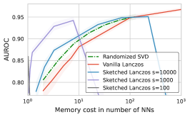
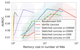
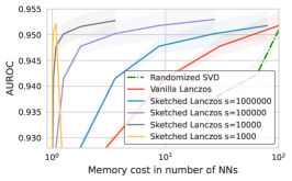
Figure 3: Sketch sizes $s$ comparison for: LeNet $p=40$K on FashionMnist vs Mnist (left), ResNet $p=300$K on Cifar-10 vs Cifar-corrupted with defocus blur (center), and VisualAttentionNet $p=4M$ on CelebA vs Food101 (right). The lower the ratio $\nicefrac{{s}}{{p}}$, the stronger the memory efficiency.

Effect of different sketch sizes. We expect the error induced by the sketching to scale as $\epsilon\approx\sqrt{k/s}$, thus a larger $k$ will have a larger error, and larger sketch sizes $s$ will have a lower error. We see the expected bell shape quite clearly in Figure 3.

[c]0.45

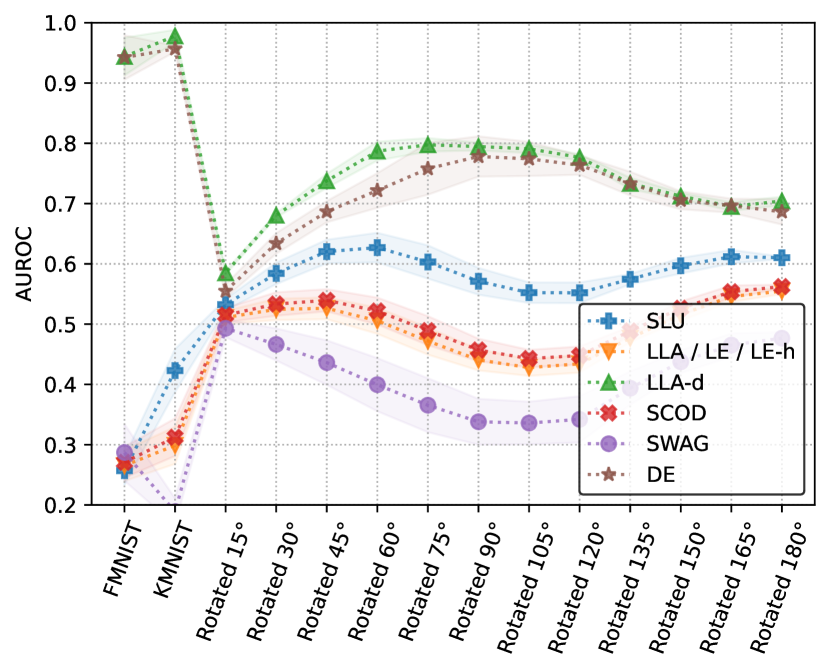
[c]0.45

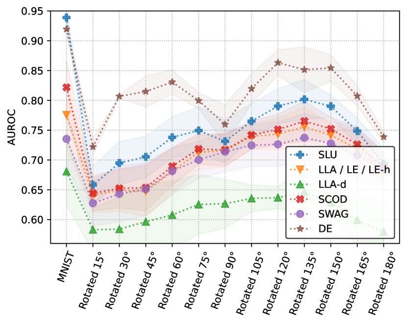
Figure 4: MLP $p=15$K trained on Mnist

Figure 5: LeNet $p=40$K trained on FashionMnist

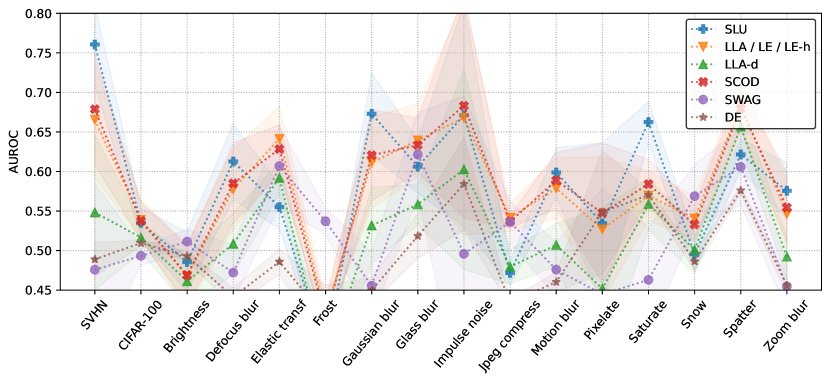
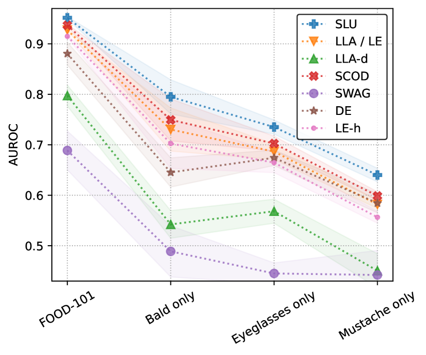
0.95 [c]0.43 [c]0.555

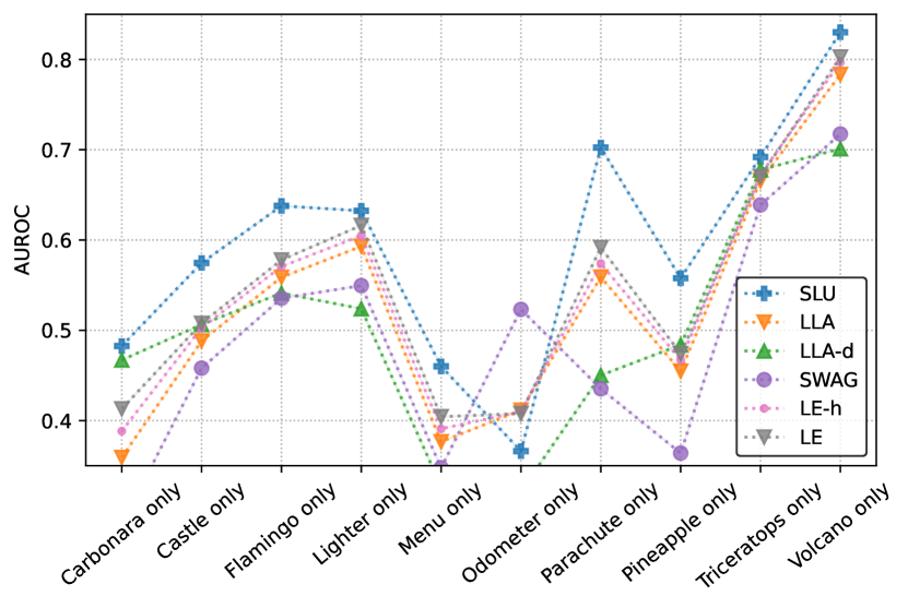
Figure 6: ResNet $p=300$K trained on Cifar-10

Figure 7: VisualAttention $p=4$M trained on CelebA

Figure 8: SWIN $p=200$M trained on ImageNet

Figure 9: AUROC scores of Sketched Lanczos Uncertainty vs baselines with memory budget $3p$.
slu outperforms the baselines on several choices of ID (9, 9, 9, 9, 9) and OoD (x-axis) datasets pairs. Dashed lines are for improved visualization only; see Table 2 for values and standard deviations. Plots 9, 9, 9, 9, 9 are averaged respectively over 10, 10, 5, 3, 1 independently trained models.

model	MLP $p=15$K			LeNet $p=40$K		ResNet $p=200$K
ID data	MNIST vs			FashionMNIST vs		CIFAR-10 vs
OoD data	FashionMNIST	KMNIST	Rotation (avg)	MNIST	Rotation (avg)	SVHN	CIFAR-100	Corrupt (avg)
slu (us)	0.26 $\pm$ 0.02	0.42 $\pm$ 0.04	0.59 $\pm$ 0.02	0.94 $\pm$ 0.01	0.74 $\pm$ 0.03	0.76 $\pm$ 0.05	0.54 $\pm$ 0.02	0.57 $\pm$ 0.04
lla	0.27 $\pm$ 0.03	0.30 $\pm$ 0.03	0.49 $\pm$ 0.01	0.80 $\pm$ 0.03	0.70 $\pm$ 0.03	0.67 $\pm$ 0.07	0.54 $\pm$ 0.02	0.57 $\pm$ 0.05
lla-d	0.94 $\pm$ 0.03	0.98 $\pm$ 0.01	0.73 $\pm$ 0.01	0.68 $\pm$ 0.07	0.61 $\pm$ 0.05	0.55 $\pm$ 0.10	0.52 $\pm$ 0.02	0.52 $\pm$ 0.04
le	0.27 $\pm$ 0.03	0.30 $\pm$ 0.03	0.49 $\pm$ 0.01	0.80 $\pm$ 0.03	0.70 $\pm$ 0.03	0.67 $\pm$ 0.07	0.54 $\pm$ 0.02	0.57 $\pm$ 0.05
le-h	0.27 $\pm$ 0.03	0.30 $\pm$ 0.03	0.49 $\pm$ 0.01	0.80 $\pm$ 0.03	0.70 $\pm$ 0.03	0.66 $\pm$ 0.07	0.54 $\pm$ 0.02	0.57 $\pm$ 0.05
scod	0.27 $\pm$ 0.03	0.31 $\pm$ 0.03	0.51 $\pm$ 0.01	0.84 $\pm$ 0.02	0.71 $\pm$ 0.03	0.68 $\pm$ 0.07	0.54 $\pm$ 0.02	0.58 $\pm$ 0.04
swag	0.29 $\pm$ 0.05	0.19 $\pm$ 0.02	0.41 $\pm$ 0.03	0.75 $\pm$ 0.02	0.70 $\pm$ 0.04	0.48 $\pm$ 0.11	0.49 $\pm$ 0.01	0.52 $\pm$ 0.06
de	0.94 $\pm$ 0.04	0.96 $\pm$ 0.00	0.71 $\pm$ 0.02	0.92 $\pm$ 0.01	0.79 $\pm$ 0.02	0.46 $\pm$ 0.02	0.51 $\pm$ 0.00	0.50 $\pm$ 0.01

model	VisualAttentionNet $p=4$M		SWIN $p=200$M
ID data	CelebA vs		ImageNet vs
OoD data	FOOD-101	Hold-out (avg)	Castle	Flamingo	Lighter	Odometer	Parachute	Pineapple	Triceratops	Volcano
slu (us)	0.95 $\pm$ 0.003	0.72 $\pm$ 0.02	0.57	0.64	0.63	0.37	0.70	0.56	0.69	0.83
lla	0.93 $\pm$ 0.001	0.67 $\pm$ 0.02	0.49	0.56	0.59	0.41	0.56	0.45	0.67	0.78
lla-d	0.80 $\pm$ 0.02	0.52 $\pm$ 0.03	0.51	0.54	0.52	0.32	0.45	0.48	0.68	0.70
le	0.93 $\pm$ 0.001	0.67 $\pm$ 0.02	0.51	0.58	0.62	0.41	0.59	0.47	0.67	0.80
le-h	0.91 $\pm$ 0.002	0.64 $\pm$ 0.03	0.50	0.57	0.60	0.41	0.57	0.47	0.67	0.80
scod	0.94 $\pm$ 0.00	0.68 $\pm$ 0.02	na	na	na	na	na	na	na	na
swag	0.69 $\pm$ 0.04	0.46 $\pm$ 0.04	0.46	0.54	0.55	0.52	0.44	0.36	0.64	0.72
de	0.88 $\pm$ 0.02	0.63 $\pm$ 0.02	na	na	na	na	na	na	na	na

Table 2: AUROC scores of Sketched Lanczos Uncertainty vs baselines with memory budget of $3p$.

Summary of the experiments.

For most of the ID-OoD dataset pairs we tested, our Sketched Lanczos Uncertainty outperforms the baselines, as shown in Table 2 and more extensively in Figure 9 where we fix the memory budget to be $3p$. Deep Ensemble performs very well in the small architecture but progressively deteriorates for bigger parameter sizes. swag outperforms the other methods on some specific choices of Cifar-10 corruptions, but we found this method to be extremely dependent on the choice of hyperparameters. scod is also a strong baseline in some settings, but we highlight that it requires instantiating the full Jacobian with an actual memory requirement of $tp$. These memory requirements make scod inapplicable to ImageNet. In this setting, given the significant training time, also Deep Ensemble becomes not applicable.

The budget of $3p$ is an arbitrary choice, but the results are consistent with different values. More experiments, including a $10p$ memory budget setting, a study on the effect of preconditioning and a synthetic-data ablation on the trade-off sketch size vs low rank, are presented in Section C.3.

6 Conclusion

We have introduced Sketched Lanczos Score, a powerful memory-efficient technique to compute approximate matrix eigendecompositions. We take a first step in exploiting this technique showing that sketching the top eigenvectors of the Generalized Gauss-Newton matrix leads to high-quality scalable uncertainty measure. We empirically show the superiority of the Sketched Lanczos Uncertainty score (slu) among a variety of baselines in the low-memory-budget setting, where the assumption is that the network has so many parameters that we can only store a few copies.

Limitations.

The data structure produced by Sketched Lanczos is sufficiently rich to evaluate the uncertainty score. However, from a Bayesian point of view, it is worth noting that the method does not allow us to sample according to the posterior.

7 OLD VERSION

8 Old Introduction

$Mio$: Maybe this Laplace details are better in the related work, they are not really useful for explaining our thing Quantifying uncertainty using local information of a single pretrained model has already proven successful. Improving over MacKay (1992), Linearized Laplace Approximation defines an uncertainty score that depends on the curvature of $f$ around $\theta^{*}$ Immer et al. (2021). Linearized Laplace score has a Bayesian interpretation as the predictive variance with respect to a Gaussian posterior, which draws connections to Gaussian Processes Khan et al. (2019). However, estimating predictive variance using second-order information incurs in the prohibitive cost of dealing with the empirical Fisher information matrix, otherwise known as Generalized Gauss Newton (ggn) Kunstner et al. (2019), which is a $p\times p$ matrix for a model with $p$ parameters.

Since computing the ggn  explicitly is intractable, several approximation techniques have been attempted. The ggn  has been approximated as block-diagonal matrix Botev et al. (2017), as a Kronecker-factorization Ritter et al. (2018b, a); Lee et al. (2020); Martens & Grosse (2015) or simply as a diagonal matrix. Other techniques restrict themselves to a subset of parameters Daxberger et al. (2021b); Kristiadi et al. (2020) or a subset of data Immer et al. (2023). Some other technique exploits connections to Neural Tangent Kernel (NTK) Deng et al. (2022).

Another technique is to approximate the ggn  as a low-rank matrix, and we look more closely into this one. A rank-$k$ approximation of the ggn  can be computed using Lanczos algorithm Madras et al. (2019); Daxberger et al. (2021a) or truncated singular value decomposition (SVD) Sharma et al. (2021). These approaches deliver promising uncertainty scores, however they are limited by their memory footprint. Indeed all aforementioned techniques require $k\cdot p$ memory. Thus, when the number of parameters $p$ is huge, $k$ must be kept small lowering the approximation quality.

In this work, we use sketching to save space and scale up the low-rank approximation method used in Madras et al. (2019). In particular, Sketched Lanczos Score  combines Lanczos algorithm with sparse sketches to compute a sketched low-rank approximation of the Fisher, which is then used to evaluate uncertainty. Whenever $k=o(\sqrt{p})$, the space complexity of Sketched Lanczos Score  is $5p$ up to lower-order terms. As shown in Figure 1 the disadvantage of introducing noise through sketching is outweighed by a higher-rank approximation, thus performing better when the same amount of memory is used.

Sketched Lanczos Score  possesses the main benefit of Linearized Laplace: it is a post-hoc method. Thus, practitioners can endow their high-performing NNs with an uncertainty estimation feature without having to re-train them nor change their highly-optimized training algorithm. As often turns out in computer science, modularity is key to success and we believe that our method takes a step further towards building an efficient, reliable and modular uncertainty estimation algorithm.

9 OLD

9.1 Sketching

The bottleneck of the pipelines in Madras et al. (2019); Sharma et al. (2021) is memory. Indeed, they store $k$ $p$-dimensional vectors, that is quite substantial when $p$ is the memory footprint of our model. The main insight of this work is that we can avoid storing these vectors explicitly and rather sketch them on the fly as they are computed. In this section, we introduce the sketching techniques that we employ in our method.

First, we define the notion of subspace embedding.

Definition 9.1 (Subspace embedding).

A $(1\pm\varepsilon)$ $\ell_{2}$-subspace embedding for the column space of an $p\times k$ matrix $U$ is a matrix $S$ for which for all $y\in\mathbb{R}^{k}$

$$\lVert SUy\rVert_{2}=(1\pm\varepsilon)\lVert Uy\rVert_{2}.$$

Our goal is to design an oblivious subspace embedding, that is a random matrix $S$ such that, for any matrix $U$, $S$ is a subspace embedding for $U$ with high enough probability. In our method, we use a Subsampled Randomized Fourier Transform (SRFT) to achieve this goal Ailon & Chazelle (2009).

A SRFT is a $s\times p$ matrix defined by the product $\frac{1}{\sqrt{sp}}PHD$, where $D$ is a diagonal matrix where each diagonal entry is an independent Rademacher random variable, $H$ is a discrete Fourier transform, and $P$ is a diagonal matrix where $s$ random diagonal entries are set to one and every other entry is set to zero. Thanks to the Fast Fourier Transform algorithm, SRFT can be evaluated in $O(p\log p)$ time, and it is apparent that its memory footprint is $p+s$.

The following theorem, shows that SRFT works as oblivious subspace embedding.

Theorem 9.2 (Essentially, Theorem 7 in Woodruff et al. (2014)).

For any $p\times k$ matrix $U$, SRFT is a $(1\pm\varepsilon)$-subspace embedding for the column space of $U$ with probability $1-\delta$ as long as $s=\Omega((k+\log p)\varepsilon^{-2}\log(k/\delta))$.

We stress that, although several other random projections work as subspace embeddings Nelson & Nguyên (2013), our choice is not incidental. Indeed other sketches, including the sparse sketches Kane & Nelson (2014); Nelson & Nguyên (2013), would either have a large memory footprint or a worse trade-off between $s$ and $k$.

$Mio$: fino a qui è andato tutto nel background

Sketching low-rank matrices.

In Madras et al. (2019), uncertainty scores are computed as the norm of $\Pi_{k}\mathbf{J}_{\theta^{*}}(q)$, where $\mathbf{J}_{\theta^{*}}(q)$ is the gradient of the query point $q$ and $\Pi_{k}=I-U_{k}U_{k}^{\top}$, where $U_{k}$ is a $p\times k$ matrix which columns are the top-$k$ eigenvector of $G$.

We observe that sketching the columns of $U_{k}$ is sufficient to recover that score approximately. In particular, the following lemma holds.

Lemma 9.3 (Sketching low-rank matrices).

Fix $0<\varepsilon,\delta<1/2$ and sample a random $s\times p$ SRFT matrix $S$. Then, for any matrix $U\in\mathbb{R}^{p\times k}$ and any unit-norm $x\in\mathbb{R}^{p}$

$$\Pr_{S}\!\Big{(}{\lVert(SU)^{\top}(Sx)\rVert_{2}=\lVert U^{\top}x\rVert_{2}\pm\varepsilon}\Big{)}>1-\delta.$$

as long as $s=\Omega((k+\log p)\varepsilon^{-2}\log(k/\delta))$.

Lemma 3.1 is a simple corollary of Theorem 2.2 and we defer its proof to the appendix.

Lemma 3.1 implies that we can store $SU_{k}$ rather than $U_{k}$, which saves significant space because $U_{k}$ has size $p\times k$ whereas $SU_{k}$ has size $\approx k\varepsilon^{-2}\times k$. Then, given a query point $q$, we compute the score of $q$ as the norm of $(S\Pi_{k})^{\top}(S\mathbf{J}_{\theta^{*}}(q))$ and we are guaranteed that this is a good approximation to the original score.

Orthogonalizing sketched vectors.

As discussed in the previous paragraph, vanilla Lanczos incurs in numerical errors, so its output vectors $V=[V_{1}|\dots|V_{k}]$ are far from being orthonormal. Orthogonalizing such vectors explicitly requires to have all of them stored in memory simultaneously, that is exactly what we are trying to avoid. Instead, we store a sketch $SV$.

Here we prove that if we orthogonalize $SV$ and apply the same orthogonalization steps to $V$, then we obtain an approximately orthonormal basis. Essentially, this means that sketching and orthogonalization approximately commute.

Lemma 9.4 (Orthogonalizing the sketch).

Fix $0<\varepsilon,\delta<1/2$ and sample a random $s\times p$ SRFT matrix $S$. As long as $s=\Omega((k+\log p)\varepsilon^{-2}\log(k/\delta))$ the following hold with probability $1-\delta$.

Given any $p\times k$ full-rank matrix $V$, decompose $V=QR$ and $SV=Q_{S}R_{S}$ so that $Q\in\mathbb{R}^{p\times k}$, $Q_{S}\in\mathbb{R}^{s\times k}$ and both $Q$ and $Q_{S}$ are semi-orthogonal. Define $\bar{Q}:=VR_{S}^{-1}$, then

$$\lVert QQ^{\top}-\bar{Q}\bar{Q}^{\top}\rVert_{2}\leq\varepsilon$$ (11)

where $\lVert\cdot\rVert_{2}$ is the operator norm.

Moreover, for each unit-norm $x\in\mathbb{R}^{p}$ we have

$$\lVert Q_{S}^{\top}(Sx)\rVert_{2}=\lVert Q^{\top}x\rVert_{2}\pm\varepsilon.$$ (12)

Proof.

Since $V$ is full-rank, it is easy to verify that $SV$ is also full rank with high probability. Thus, $R$ is non-singular and $\bar{Q}=VR_{S}^{-1}$ is well-defined. Notice that $Q_{S}=S\bar{Q}$. We prove that $\bar{Q}$ is approximately orthonormal. By definition of $Q_{S}$, we have $I_{k}=Q_{S}^{\top}Q_{S}=\bar{Q}S^{\top}S\bar{Q}^{\top}$ By subspace embedding property of $S$, we have that

$$\lVert\bar{Q}\bar{Q}^{\top}-I_{k}\rVert_{2}=\lVert\bar{Q}\bar{Q}^{\top}-\bar{Q}S^{\top}S\bar{Q}^{\top}\rVert_{2}\leq\varepsilon$$

with probability $1-\delta$. Conditioning on this event, the singular values of $\bar{Q}$ lie in $[1-\varepsilon,1+\varepsilon]$. Moreover, $Ran(Q)=Ran(\bar{Q})$. Therefore, taking the singular value decomposition (SVD) of $Q$ and $\bar{Q}$ yields Equation 13.

Let $x\in\mathbb{R}^{p}$ be an arbitrary unit norm vector. Now we are left to prove that $\lVert\bar{Q}^{\top}x\rVert_{2}=\lVert Q_{S}^{\top}Sx\rVert_{2}$. We have $Q_{S}^{\top}S=\bar{Q}^{\top}S^{\top}S$ and by Lemma 3.1 we have $\lVert\bar{Q}^{\top}S^{\top}Sx\rVert_{2}=\lVert\bar{Q}^{\top}x\rVert_{2}\pm\varepsilon$ with probability $1-\delta$. Thus, $\lVert\bar{Q}^{\top}x\rVert_{2}=\lVert Q_{S}^{\top}Sx\rVert_{2}\pm\varepsilon$ and combined with Equation 13 gives Equation 12, up to constant blow-ups in $\varepsilon$ and $\delta$.

∎

$Mio$: spiegare che $R_{S}^{-1}$ è l’algoritmo di orthogonalizzazione imparato sugli sketed vector, ma poi lo applichiamo (teoricamente, non praticamente) ai non sketched

Appendix A Dimensionality Reduction

A.1 Proof of “Sketching low-rank matrices" Lemma

In this section, we prove Lemma 3.1. We restate it below for convenience. See 3.1

Proof.

In order to prove that $||(SU)^{\top}(Sv)||_{2}=||U^{\top}v||_{2}\pm\varepsilon$ with probability $\geq 1-\delta$ we prove the following stronger statement. Denote with $[u]_{i}$ the $i$-th coordinae of $u$, then for each $i=1\dots k$ we have $[(SU)^{\top}(Sv)]_{i}=[U^{\top}v]_{i}\pm\varepsilon/\sqrt{k}$ with probability at least $1-\delta/k$. Apparently, the former follows from the latter by union bound.

Notice that $[(SU)^{\top}(Sv)]_{i}=(SU^{i})^{\top}(Sv)$, where $U^{i}$ is the $i$-th column of $U$. Moreover, as long as $s=\Omega(k\varepsilon^{-2}\cdot\log p\cdot\log(k/\delta))$, then $S$ is a $(1\pm\varepsilon/\sqrt{k})$-subspace embedding for the $2$-dimensional subspace spanned by $v$ and $U^{i}$ with probability $1-\delta/k$ (Theorem 2.2). Therefore, conditioning on this event:

$$(SU^{i})^{\top}(Sv) =\frac{1}{4}\left(||S(U^{i}+v)||^{2}_{2}-||S(U^{i}-v)||^{2}_{2}\right)$$

$$=\frac{1}{4}\left(||(U^{i}+v)||^{2}_{2}-||(U^{i}-v)||^{2}_{2}\right)\pm O(\varepsilon/\sqrt{k})$$

$$=(U^{i})^{\top}v\pm O(\varepsilon/\sqrt{k})$$

$$=[U^{\top}v]_{i}\pm O(\varepsilon/\sqrt{k}).$$

The second equality sign holds because of the subspace embedding property, together with $||U^{i}+v||_{2},||U^{i}-v||_{2}=O(1)$. ∎

A.2 Proof of “Orthogonalizing the sketch" Lemma

In this section, we prove Lemma 3.2. We restate it below for convenience.

See 3.2

Proof.

Since $V$ is full-rank, it is easy to verify that $SV$ is also full rank with high probability. Thus, $R$ is non-singular and we can define $\bar{U}=VR_{S}^{-1}$. Notice that $U_{S}=S\bar{U}$. Now, we prove that

$$\lVert UU^{\top}-\bar{U}\bar{U}^{\top}\rVert_{2}\leq\varepsilon$$ (13)

where $\lVert\cdot\rVert_{2}$ is the operator norm. By definition of $U_{S}$, we have $I_{k}=U_{S}^{\top}U_{S}=\bar{U}S^{\top}S\bar{U}^{\top}$ By subspace embedding property of $S$, we have that

$$\lVert\bar{U}\bar{U}^{\top}-I_{k}\rVert_{2}=\lVert\bar{U}\bar{U}^{\top}-\bar{U}S^{\top}S\bar{U}^{\top}\rVert_{2}\leq\varepsilon$$

with probability $1-\delta$. Conditioning on this event, the singular values of $\bar{U}$ lie in $[1-\varepsilon,1+\varepsilon]$. Moreover, $Ran(U)=Ran(\bar{U})$. Therefore, taking the singular value decomposition (SVD) of $U$ and $\bar{U}$ yields Equation 13.

Now we are left to prove that $\lVert\bar{U}^{\top}v\rVert_{2}=\lVert U_{S}^{\top}Sv\rVert_{2}\pm\varepsilon$. We have $U_{S}^{\top}S=\bar{U}^{\top}S^{\top}S$ and by Lemma 3.1 we have $\lVert\bar{U}^{\top}S^{\top}Sv\rVert_{2}=\lVert\bar{U}^{\top}v\rVert_{2}\pm\varepsilon$ with probability $1-\delta$. Thus, $\lVert\bar{U}^{\top}v\rVert_{2}=\lVert U_{S}^{\top}Sv\rVert_{2}\pm\varepsilon$ and combined with Equation 13 gives Equation 12, up to constant blow-ups in $\varepsilon$ and $\delta$. ∎

A.3 Extension of Lemma 3.2

In this section we extend Lemma 3.2 to the case where instead of having a query vector $v\in\mathbb{R}^{p}$ we have a query matrix $J\in\mathbb{R}^{p\times t}$. In our application, $J$ is the Jacobian $\mathbf{J}_{\theta^{*}}(q)$.

Lemma A.1 (Orthogonalizing the sketch, for matrix queries).

Fix $0<\varepsilon,\delta<1/2$ and sample a random $s\times p$ SRFT matrix $S$. As long as $s=\Omega(tk\varepsilon^{-2}\cdot\log p\cdot\log(tk/\delta))$ the following holds with probability $1-\delta$.

Given any $p\times k$ full-rank matrix $V$, decompose $V=UR$ and $SV=U_{S}R_{S}$ so that $U\in\mathbb{R}^{p\times k}$, $U_{S}\in\mathbb{R}^{s\times k}$ and both $U$ and $U_{S}$ have orthonormal columns. For any $J\in\mathbb{R}^{p\times t}$ we have

$$\lVert J\rVert^{2}_{F}-\lVert U_{S}^{\top}(SJ)\rVert^{2}_{F}=(1\pm\varepsilon)\lVert J\rVert^{2}_{F}-\lVert U^{\top}J\rVert^{2}_{F}.$$ (14)

Proof.

Let $J^{i}$ the $i$-th column of $J$. Suppose that the following intermediate statement holds: for each $i$, $\lVert U_{S}^{\top}(SJ^{i})\rVert_{2}=\lVert U^{\top}J^{i}\rVert_{2}\pm\lVert J\rVert_{F}\cdot\varepsilon/\sqrt{t}$ with probability $1-\delta/t$. If the statement above holds, then we have

$$|\lVert U_{S}^{\top}(SJ)\rVert^{2}_{F}-\lVert U^{\top}J\rVert^{2}_{F}| =$$

$$(\lVert U_{S}^{\top}(SJ)\rVert_{F}+\lVert U^{\top}J\rVert_{F})\cdot|\lVert U_{S}^{\top}(SJ)\rVert_{F}-\lVert U^{\top}J\rVert_{F}| \leq$$

$$O(\lVert J\rVert_{F})\cdot\sqrt{\sum_{i}(\lVert U_{S}^{\top}(SJ^{i})\rVert_{2}-\lVert U^{\top}J^{i}\rVert_{2})^{2}} \leq$$

$$O(\lVert J\rVert_{F}^{2}\cdot\varepsilon).$$

The penultimate inequality holds because of triangle inequality, whereas the last inequality holds with probability $1-\delta$ by union bound.

To prove the intermediate statement above, it is sufficient to apply Lemma 3.2 with $\varepsilon^{\prime}=\varepsilon/\sqrt{t}$ and $\delta^{\prime}=\delta/t$. ∎

Appendix B Lanczos algorithm

Lanczos algorithm is an iterative method for tridiagonalizing an Hermitian matrix $G$. If stopped at iteration $k$, Lanczos returns a column-orthogonal matrix $V=[V_{1}|\dots|V_{k}]\in\mathbb{R}^{p\times k}$ and a tridiagonal matrix $T\in\mathbb{R}^{k\times k}$ such that $V^{\top}GV=T$. The range space of $V$ corresponds to the Krylov subspace $\mathcal{K}_{k}=span\{v,Gv,\dots,G^{k-1}v\}$, where $v=V_{1}$ is a randomly chosen vector. Provably $\mathcal{K}_{k}$ approximates the eigenspace spanned by the top-$k$ eigenvectors (those corresponding to eigenvalues of largest modulus) of $G$. Thus, $VTV^{\top}$ approximates the projection of $G$ onto its top-$k$ eigenspace. Notice that projecting $G$ onto its top-$k$ eigenspace yields the best rank-$k$ approximation of $G$ under any unitarily-invariant norm Mirsky (1960). Moreover, as observed in the previous section the spectrum of the ggn  decays rapidly, making low-rank decomposition particularly accurate.

Once the decomposition $G\approx VTV^{\top}$ is available, we can retrieve an approximation to the top-$k$ eigenpairs of $G$ by diagonalizing $T$ into $T=W\Lambda W^{\top}$, which can be done efficiently for tridiagonal matrices Dhillon (1997). The quality of eigenpairs’ approximation has been studied in theory and practice. We point the reader to Meurant (2006); Cullum & Willoughby (2002) for a comprehensive sourvey on this topic.

Lanczos, in a nutshell.

Here we give a minimal description of Lanczos algorithm. Lanczos maintains a set of vectors $V=[V_{1}|\dots|V_{k}]$, where $V_{1}$ is initialized at random. At iteration $i+1$, Lanczos performs a matrix-vector product $V_{i+1}\leftarrow G\cdot V_{i}$, orthogonalizes $V_{i+1}$ against $V_{i}$ and $V_{i-1}$ and normalizes it. The tridiagonal entries of $T$ are given by coefficients computed during orthogonalization and normalization. See Chapter 1 of Meurant (2006) for a full description of Lanczos algorithm.

The benefits of Lanczos.

Lanczos has two features that make it particularly appealing for our uses case. First, Lanczos does not need explicit access to the input matrix $G$, but only access to an implementation of $u\mapsto Gu$. Second, Lanczos uses a small working space: only $3p$ floating point numbers, where the input matrix is $p\times p$. Indeed, we can think of Lanczos as releasing its output in streaming and only storing a tiny state consisting of the last three vectors $V_{i-1},V_{i}$ and $V_{i+1}$.

The curse of numerical instability.

Unfortunately, the implementation of Lanczos described above is prone to numerical instability, causing $V_{1}\dots V_{k}$ to be far from orthogonal. A careful analysis of the rounding errors causing this pathology was carried out by Paige in his PhD thesis as well as a series of papers Paige (1971, 1976, 1980).

To counteract this, a standard technique is to re-orthogonalize $V_{i+1}$ against all $\{V_{j}\}_{j\leq i}$, at each iteration. This technique has been employed to compute the low-rank approximation of huge sparse matrices Simon & Zha (2000), as well as in Madras et al. (2019) to compute an approximation to the top-$k$ eigenvectors. Unfortunately, this version of Lanczos loses one the two benefits described above, in that it must store a larger state consisting of the whole matrix $V$. Therefore, we dub this version of thew algorithm hi-memory Lanczos and the cheaper version described above low-memory Lanczos .

Paige Paige (1980) proved that the loss of orthogonality in low-memory Lanczos is strictly linked to the convergence of some of the approximate eigenpairs to the corresponding eigenpairs of $G$. Moreover, the vectors $V_{1}\dots V_{k}$ are not orthogonal because they are tilted towards such eigenpairs. Accordingly, he observed that among the eigenpairs computed by low-memory Lanczos there are multiple eigenpairs approximating the same eigenpair of $G$. This can easily be observed while running both low-memory Lanczos and hi-memory Lanczos and computing the dot products of the their retrieved eigenvectors; see Figure 10.

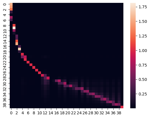
Figure 10: We study the ggn  of a LeNet model with $44.000$ parameters trained on MNIST. We run $40$ iterations of hi-memory Lanczos and low-memory Lanczos . Let $H=[H_{1}|\dots|H_{40}]$, $\Lambda_{H}$, $L=[L_{1}|\dots|L_{40}]$, and $\Lambda_{L}$ be the eigenvectors and eigenvalues computed by the two algorithms respectively. We sort both sets of eigenvectors in decreasing order of corresponding eigenvalues. In position $(i,j)$ we plot $\langle H_{i},L_{j}\rangle$. It is apparent that multiple eigenvectors $L_{j}$ correspond to the same eigenvector $H_{i}$.

Post-hoc orthogonalization.

Based on the observations of Paige Paige (1980), we expect that orthogonalizing the output of low-memory Lanczos post-hoc should yield an orthonormal basis that approximately spans the top-$k$ eigenspace. Since in our method we only need to project vectors onto the top-$k$ eigenspace, this suffices to our purpose.

We confirm this expectation empirically. Indeed, using the same setting of Figure 10 we define $\Pi_{LM}$ as the projection onto the top-$10$ principal components of $L\Lambda_{L}$, and define $\Pi_{HM}$ likewise. Then, we measure the operator norm (i.e., the largest singular value) of $\Pi_{LM}-\Pi_{HM}$ and verify that it is fairly low, only $0.03$. Taking principal components was necessary, because there is no clear one-to-one correspondence between $L_{i}$s and $H_{i}$s, in that as observed in Figure 10 many $L_{i}$s can correspond to a single $H_{i}$. Nonetheless, this proves that low-memory Lanczos is capable of approximating the top eigenspace.

B.1 Spectral properties of the Hessian /ggn

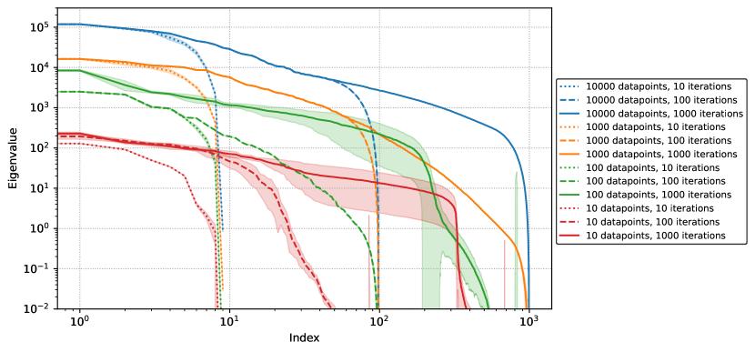
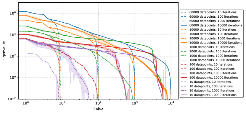
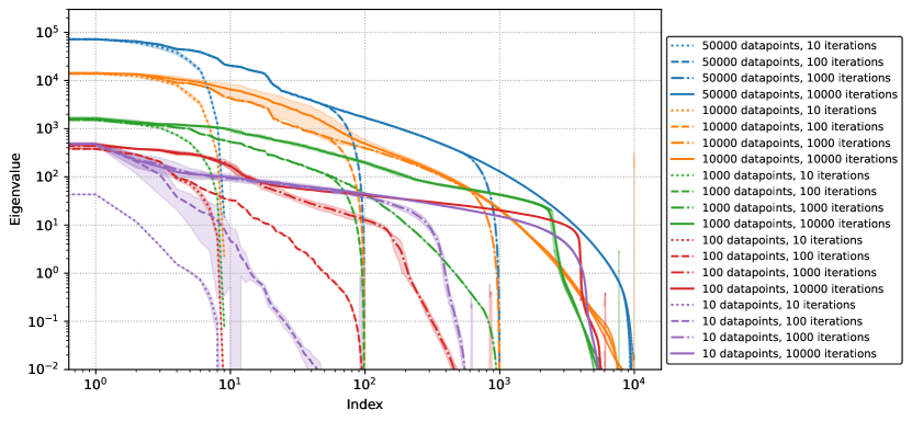
Figure 11: Eigenspectrum obtained from hi-memory Lanczos on: ResNet model ($p=300$K) trained on CIFAR-10 (top), LeNet model ($p=40$K) trained on FashionMNIST (middle) and MLP model ($p=20$K) trained on MNIST (bottom).

Spectral property of the ggn  and Hessian have been studied both theoretically and empirically. In theory, it was observed that in the limit of infinitely-wide NN, the Hessian is constant through training Jacot et al. (2018). However, this is no longer true if we consider NN with finite depth Lee et al. (2019). In Sagun et al. (2017); Papyan (2018); Ghorbani et al. (2019), they show empirically that the spectrum of the ggn  / Hessian is composed of two components: a bulk of near-zero eigenvalues, and a small fraction of outliers away from the bulk. Moreover, in Ghorbani et al. (2019), they observe a large concentration of the gradients along the eigenspace corresponding to the outlier eigenvalues.

In summary, the spectrum of the ggn  / Hessian of a deep NN is expected to decay rapidly, having a few outlier eigenvalues, along which most gradients are oriented. Therefore, we would expect a low-rank approximation of the ggn  to capture most relevant information.

We test this phenomenon by using hi-memory Lanczos and performing an ablation over both number of iterations and random initialization of the first vector. Figure 11 shows the results over three different model trained on different datasets. The plots cointains means and std bars over 5 random initializations of the first Lanczos vector. It is interesting to observe how, varying the number of iterations, approximately the first 90% values are the same, while the tail quickly drop down to numerical precision. Based on this observation we choose to only use the top 90% vectors returned by Lanczos.

Appendix C Experimental setting and extended results

Experiments are reproducible and the code is available at https://github.com/IlMioFrizzantinoAmabile/uncertainty_quantification. As explained later in greater details, calling the scripts train_model.py and score_model.py with the right parameters is enough to reproduce all the numbers we presented.

Reproducibility. The script bash/plot_figure_4.sh collects the entire pipeline of setup, training, scoring and plotting and finally reproduce Figure 9 (all three plots) and save them in the folder figures. The script takes approximately 3 days to complete on a NVIDIA H100 80GB GPU.

The code is implemented in JAX (jax2018github) in order to guarantee max control on the randomness, and, given a trained model and a random seed, the scoring code is fully deterministic (and thus fully reproducible). Nonetheless, the dataloader shuffling used at training time depends on PyTorch (bad) randomness management, and consequently it can be machine-dependent.

C.1 Training details

All experiments were conducted on models trained on one of the following datasets: Mnist (Lecun et al., 1998), FashionMnist (Xiao et al., 2017), Cifar-10 (cifar10), CelebA (Liu et al., 2015) and ImageNet (deng2009imagenet). Specifically we train:

• on Mnist with a MLP consisting of one hidden layer of size 20 with tanh activation functions, we trained with ADAM for 50 epochs with a batch size 128 and a learning rate $10^{-3}$; parameter size is $p=15910$;

• on FashionMnist with a LeNet consisting of two convolution layers with maxpool followed by 3 fully connected layers with tanh activation functions, we trained with ADAM for 50 epochs with a batch size 128 and a learning rate $10^{-3}$; parameter size is $p=44426$;

• on Cifar-10 with a ResNet with $(3,3,3)$ blocks of channel sizes $(16,32,64)$ with relu activation functions, we trained with SGD for 200 epochs with a batch size 128 and a learning rate $0.1$, momentum $0.9$ and weight decay $10^{-4}$; parameter size is $p=272378$;

• on CelebA with a VisualAttentionNetwork with blocks of depths $(3,3,5,2)$ and embedded dimensions of $(32,64,160,256)$ with relu activation functions, we trained with Adam for 50 epochs with a batch size 128 and a learning rate decreasing from $10^{-3}$ to $10^{-5}$; parameter size is $p=3858309$.

• on ImageNet with a SWIN model with an embed dimension of $192$, blocks of depths $(2,2,18,2)$ and number of heads $6,12,24,48)$, we trained with Adam with weight decay for 60 epochs plus a 10 epoch warmup, with a batch size 128 and a learning rate decreasing from $10^{-3}$ to $10^{-5}$; parameter size is $p=196517106$.

For training and testing the default splits were used. All images were normalized to be in the $[0,1]$ range. For the CelebA dataset we scale the loss by the class frequencies in order to avoid imbalances. The cross entropy loss was used as the reconstruction loss in the first three models, while multiclass binary cross entropy was used for the last one.

We train all models with 10 different random seed, (except for ImageNet, that we only trained with one seed) which can be reproduced by running [language=bash] bash/setup.sh source virtualenv/bin/activate echo "Train all models" for seed in 1..10 do python train_model.py –dataset MNIST –likelihood classification –model MLP –seed $seed--run_{n}amegood--default_{h}yperparamspythontrain_{m}odel.py--datasetFMNIST--likelihoodclassification--modelLeNet--seed$seed –run_name good –default_hyperparams python train_model.py –dataset CIFAR-10 –likelihood classification –model ResNet –seed $seed--run_{n}amegood--default_{h}yperparamspythontrain_{m}odel.py--datasetCelebA--likelihoodbinary_{m}ulticlassification--modelVAN_{t}iny--seed$seed –run_name good –default_hyperparams python train_model.py –dataset ImageNet –likelihood classification –model SWIN_large –seed $seed--run_{n}amegood--default_{h}yperparamsdoneThetrainedmodel\emph{test set}accuraciesare:$0.952±0.001,0.886±0.003,0.911±0.003,0.889±0.002,0.672$,respectivelyforthe5differentsettings.\par\par$

C.2 Scoring details

The standard deviations of the scores presented are obtained scoring the indepentently trained models. For all methods we use: 5 seeds for MNIST, 10 seeds for FMNIST, 5 seeds for CIFAR-10 and 3 seeds for CelebA. The only exception is Deep Ensemble for which we used only 3 independent scores for the budget3 experiment (for a total of 9 models used) and only 1 score for the budget10 experiments (using all the 10 trained model).

For the fixed memory budget experiments we fix the rank $k$ to be equal to the budget (3 or 10) for all baseline, while for our method we were able to have a higher rank thanks to the memory saving induced by sketching, specifically:

• for experiments with MNIST as in-distribution we used a sketch size $s=1000$ and a rank $k=45$ for the budget3 and $k=150$ for the budget10;

• for experiments with FashionMNIST as in-distribution we used a sketch size $s=1000$ and a rank $k=132$ for the budget3 and $k=440$ for the budget10;

• for experiments with CIFAR-10 as in-distribution we used a sketch size $s=10000$ and a rank $k=81$ for the budget3 and a sketch size $s=50000$ and a rank $k=50$ for the budget10;

• for experiments with CelebA as in-distribution we used a sketch size $s=10000$ and a rank $k=100$ both for the budget3 and for the budget10.

• for experiments with ImageNet as in-distribution we used a sketch size $s=20000000$ and a rank $k=30$.

Baseline-specific details:

• swag: we set the parameter collecting frequency to be once every epoch; we perform a grid search on momentum and learning rate hyperparameter: momentum in $[0.9,0.99]$ resulting in the latter being better, and learning rate in $[0.1,1,10]$ times the one used in training resulting in 1 being better. Although we spent a decent amount of effort in optimizing these, it is likely that a more fine search may yield slighlty better results;

• scod: the truncated randomized SVD has a parameter $T$ and we refer to the paper for full explanation. Importantly to us, the default value is $T=6k+4$ and the memory usage at preprocessing is $Tp$, which is greater than $kp$. Nonetheless at query time the memory requirement is $pk$ and we consider only this value in order to present the score in the most fair way possible;

• Local Ensemble: the method presented in the original paper actually makes use of the Hessian, rather than the GGN. And we denoted them as le-h and le respectively, which is not fully respectful of the original paper but we think this approach helps clarity. Anyway, we extensively test both variant and the resulting tables show that they always perform the same up to 2 decimal;

• Deep Ensemble: each ensemble consists of either 3 or 10 models, depending on the experiment, each initialized with a different random seed;

• Diagonal Laplace: has a fixed memory requirement of $1p$.

All the scores relative to the budget3 experiment on CIFAR-10 reported in Table 2 can be reproduced by running the following bash code [language=bash] bash/setup.sh source ./virtualenv/bin/activate dataset="CIFAR-10" ood_datasets="SVHN CIFAR-100 CIFAR-10-C" model_name="ResNet" for seed in 1..5 do echo "Sketched Lanczos" python score_model.py –ID_dataset $dataset--OOD_{d}atasets$ood_datasets –model $model_{n}ame--model_{s}eed$seed –run_name good –subsample_trainset 10000 –lanczos_hm_iter 0 –lanczos_lm_iter 81 –lanczos_seed 1 –sketch srft –sketch_size 10000 echo "Linearized Laplace" python score_model.py –ID_dataset $dataset--OOD_{d}atasets$ood_datasets –model $model_{n}ame--model_{s}eed$seed –run_name good –subsample_trainset 10000 –lanczos_hm_iter 3 –lanczos_lm_iter 0 –lanczos_seed 1 –use_eigenvals echo "Local Ensembles" python score_model.py –ID_dataset $dataset--OOD_{d}atasets$ood_datasets –model $model_{n}ame--model_{s}eed$seed –run_name good –subsample_trainset 10000 –lanczos_hm_iter 3 –lanczos_lm_iter 0 –lanczos_seed 1 echo "Local Ensemble Hessian" python score_model.py –ID_dataset $dataset--OOD_{d}atasets$ood_datasets –model $model_{n}ame--model_{s}eed$seed –run_name good –subsample_trainset 10000 –lanczos_hm_iter 3 –lanczos_lm_iter 0 –lanczos_seed 1 –use_hessian echo "Diag Laplace" python score_model.py –ID_dataset $dataset--OOD_{d}atasets$ood_datasets –model $model_{n}ame--model_{s}eed$seed –run_name good –score diagonal_lla –subsample_trainset 10000 echo "SCOD" python score_model.py –ID_dataset $dataset--OOD_{d}atasets$ood_datasets –model $model_{n}ame--model_{s}eed$seed –run_name good –score scod –n_eigenvec_hm 3 –subsample_trainset 10000 echo "SWAG" python score_model.py –ID_dataset $dataset--OOD_{d}atasets$ood_datasets –model $model_{n}ame--model_{s}eed$seed –run_name good –score swag –swag_n_vec 3 –swag_momentum 0.99 –swag_collect_interval 1000 done for seed in (1,4,7) echo "Deep Ensembles" python score_model.py –ID_dataset $dataset--OOD_{d}atasets$ood_datasets –model $model_{n}ame--model_{s}eed$seed –run_name good –score ensemble –ensemble_size 3 do done

Disclaimer. We did not include the KFAC approximation as a baseline, although its main selling point is the memory efficiency. The reason is that it is a layer-by-layer approximation (and so it neglects correlation between layers) and its implementation is layer-dependent. There exist implementations for both linear layers and convolutions, which makes the method applicable to MLPs and LeNet. But, to the best of our knowledge, there is no implementation (or even a formal expression) for skip-connections and attention layers, consequently making the method inapplicable to ResNet, Visual Transformer, or more complex architectures.

Disclaimer 2. We did not include the max logit values (Hendrycks & Gimpel, 2016) as a baseline. The reason is that it is only applicable for classification tasks, so for example would not be applicable for CelebA which is a binary multiclassfication task.

Out-of-Distribution datasets.

In an attempt to evaluate the score performance as fairly as possible, we include a big variety of OoD datasets. For models trained on MNIST we used the rotated versions of MNIST, and similarly for FashionMNIST. We also include KMNIST as an MNIST-Out-of-Distribution. For models trained on CIFAR-10 we used CIFAR-100, svhn and the corrupted versions of CIFAR-10, of the 19 corruption types available we only select and present the 14 types for which at least one method achieve an auroc$\geq 0.5$. For models trained on CelebA we used the three subsets of CelebA corresponding to faces with eyeglasses, mustache or beard. These images were of course excluded from the In-Distribution train and test dataset. Similarly for models trained on ImageNet we used excluded from the In-Distribution train and test dataset 10 classes (Carbonara, Castle, Flamingo, Lighter, Menu, Odometer, Parachute, Pineapple, Triceratops, Volcano) and use them as OoD datasets. We do not include the results for Carbonara and Menu since no method was able to achive an auroc$\geq 0.5$.

Note that rotations are meaningful only for MNIST and FashionMNIST since other datasets will have artificial black padding at the corners which would make the OoD detection much easier.

C.3 More experiment

Here we present more experimental results. Specifically we perform an ablation on sketch size $s$ in Section C.3.1 (on synthetic data) and on preconditioning size in Section C.3.2. Then in Section C.3.3 we perform again all the experiments in Figure 9, where the budget is fixed to be $3p$, but now with a higher budget of $10p$. We score the 62 pairs ID-OoD presented in the previous section (each pair correspond to a x-position in the plots in Figure 18), with the exception of ImageNet because a single H100 GPU is not enough for it.

C.3.1 Synthetic data

Here we motivate the claim “the disadvantage of introducing noise through sketching is outweighed by a higher-rank approximation" with a synthetic experiment. For a fixed “parameter size" $p=10^{6}$ and a given ground-truth rank $R=100$ we generate an artificial Fisher matrix $M$. To do so, we sample $R$ uniformly random orthonormal vectors $v_{1}\dots v_{R}\in\mathbb{R}^{p}$ and define $M=\sum_{i}\lambda_{i}v_{i}v_{i}^{\top}$ for some $\lambda_{i}>0$. Doing so allows us to (1) implement $x\mapsto Mx$ without instantiating $M$ and (2) have explicit access to the exact projection vector product so we can measure both the sketch-induded error and the lowrank-approximation-induced error, so we can sum them and observe the trade-off.

For various values of $k$ (on x-axis) and $s$ (on y-axis), we run Skeched Lanczos on $x\mapsto Mx$ for $k$ iteration with a sketch size $s$, and we obtain the sketched low rank approximation $U_{S}$. To further clarify, on the x-axis we added the column “inf" which refers to the same experiments done without any sketching (thus essentially measuring Lanczos lowrank-approximation-error only) which coincides with the limit of $s\rightarrow\infty$. The memory requirement of this “inf" setting is $Pk$, that is the same as the second to last column where $s=P$.

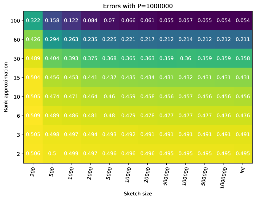
Figure 12: Ablation on rank $k$ and sketch size $s$.

We generate a set of test Jacobians as random unit vectors conditioned on their projection onto $Span(v_{1}\dots v_{R})$ having norm $\frac{1}{\sqrt{2}}$. We compute their score both exacltly (as in Equation 9) and sketched (as in Equation 10). In the Figure we show the difference between these two values. As expected, higher rank $k$ leads to lower error, and higher sketch size $s$ leads to lower error. Note that the memory requirement is proportional to the product $ks$, and the figure is in log-log scale.

C.3.2 Effect of different preconditioning sizes

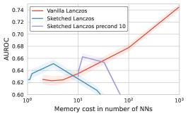
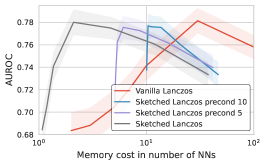
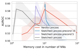
Figure 13: Preconditioning comparison for LeNet $p=40$K on FashionMnist vs FashionMnist-rotated-30° (left), and ResNet $p=300$K on Cifar-10 vs Svhn (center) or Cifar-pixelated (right).

Preconditioning can be thought of as a smooth bridge between high-memory Lanczos and Sketched Lanczos. We run the former for a few steps and then continue with the latter on the preconditioned matrix. Consequently, the preconditioning scores “start” from the vanilla Lanczos curve, and improve quicker memory-wise, as shown in Figure 13.

C.3.3 Budget 10

The results with memory bugdet $10p$ are in Table 3, Table 4 and more extensively in Figure 18.

	MNIST			FashionMNIST
	vs			vs
	FashionMNIST	KMNIST	Rotation (avg)	MNIST	Rotation (avg)
slu (us)	0.28 $\pm$ 0.02	0.46 $\pm$ 0.04	0.61 $\pm$ 0.02	0.95 $\pm$ 0.01	0.75 $\pm$ 0.03
lla	0.27 $\pm$ 0.03	0.34 $\pm$ 0.03	0.52 $\pm$ 0.01	0.88 $\pm$ 0.03	0.72 $\pm$ 0.03
lla-d	0.94 $\pm$ 0.03	0.98 $\pm$ 0.01	0.73 $\pm$ 0.01	0.68 $\pm$ 0.06	0.61 $\pm$ 0.04
le	0.27 $\pm$ 0.03	0.34 $\pm$ 0.03	0.52 $\pm$ 0.01	0.88 $\pm$ 0.03	0.72 $\pm$ 0.03
le-h	0.27 $\pm$ 0.03	0.34 $\pm$ 0.03	0.52 $\pm$ 0.01	0.88 $\pm$ 0.03	0.72 $\pm$ 0.03
scod	0.27 $\pm$ 0.02	0.36 $\pm$ 0.03	0.54 $\pm$ 0.01	0.89 $\pm$ 0.02	0.72 $\pm$ 0.03
swag	0.26 $\pm$ 0.05	0.18 $\pm$ 0.03	0.39 $\pm$ 0.03	0.77 $\pm$ 0.04	0.72 $\pm$ 0.04
de	0.90	1.00	0.79	0.99	0.90

Table 3: AUROC scores of Sketched Lanczos Uncertainty vs baselines with a memory budget of $10p$.

	CIFAR-10			CelebA
	vs			vs
	SVHN	CIFAR-100	Corruption (avg)	food-101	Hold-out (avg)
slu (us)	0.76 $\pm$ 0.06	0.54 $\pm$ 0.02	0.57 $\pm$ 0.04	0.95 $\pm$ 0.003	0.72 $\pm$ 0.02
lla	0.72 $\pm$ 0.06	0.53 $\pm$ 0.02	0.57 $\pm$ 0.04	0.94 $\pm$ 0.001	0.70 $\pm$ 0.02
lla-d	0.55 $\pm$ 0.10	0.52 $\pm$ 0.02	0.52 $\pm$ 0.04	0.80 $\pm$ 0.02	0.52 $\pm$ 0.03
le	0.72 $\pm$ 0.06	0.53 $\pm$ 0.02	0.57 $\pm$ 0.04	0.94 $\pm$ 0.001	0.70 $\pm$ 0.02
le-h	0.72 $\pm$ 0.07	0.53 $\pm$ 0.02	0.57 $\pm$ 0.04	0.93 $\pm$ 0.002	0.67 $\pm$ 0.02
scod	0.75 $\pm$ 0.05	0.54 $\pm$ 0.02	0.58 $\pm$ 0.04	0.94 $\pm$ 0.002	0.70 $\pm$ 0.02
swag	0.52 $\pm$ 0.06	0.44 $\pm$ 0.02	0.51 $\pm$ 0.05	0.78 $\pm$ 0.13	0.55 $\pm$ 0.09
de	0.45	0.51	0.50	0.96	0.68

Table 4: AUROC scores of Sketched Lanczos Uncertainty vs baselines with a memory budget of $10p$.

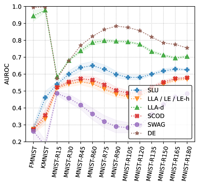
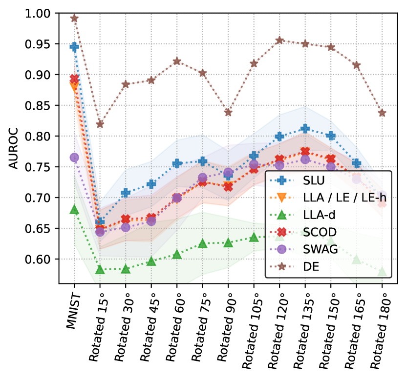
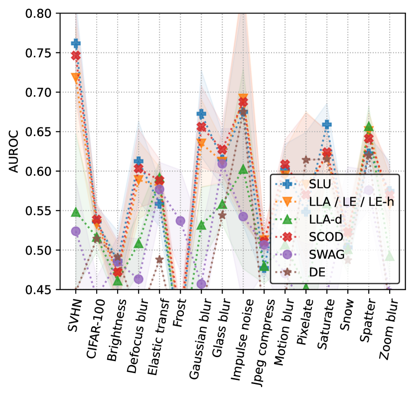
[c]0.47 [c]0.47 [c]0.47 [c]0.47

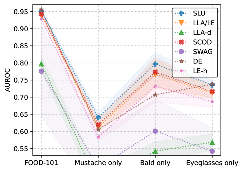
Figure 14: MLP $p=15$K train on MNIST

Figure 15: LeNet $p=40$K train on FMNIST

Figure 16: ResNet $p=300$K train on CIFAR-10

Figure 17: VAN $p=4$M train on CelebA

Figure 18: AUROC scores of Sketched Lanczos Uncertainty vs baselines with a memory budget of $10p$.

References

- Ailon & Chazelle (2009) Ailon, N. and Chazelle, B. The fast johnson–lindenstrauss transform and approximate nearest neighbors. SIAM Journal on computing, 39(1):302–322, 2009.
- Antorán et al. (2022) Antorán, J., Padhy, S., Barbano, R., Nalisnick, E., Janz, D., and Hernández-Lobato, J. M. Sampling-based inference for large linear models, with application to linearised laplace. arXiv preprint arXiv:2210.04994, 2022.
- Blundell et al. (2015) Blundell, C., Cornebise, J., Kavukcuoglu, K., and Wierstra, D. Weight uncertainty in neural network. In International conference on machine learning, pp. 1613–1622. PMLR, 2015.
- Botev et al. (2017) Botev, A., Ritter, H., and Barber, D. Practical gauss-newton optimisation for deep learning. In International Conference on Machine Learning, pp. 557–565. PMLR, 2017.
- Cullum & Willoughby (2002) Cullum, J. K. and Willoughby, R. A. Lanczos algorithms for large symmetric eigenvalue computations: Vol. I: Theory. SIAM, 2002.
- Daxberger et al. (2021a) Daxberger, E., Kristiadi, A., Immer, A., Eschenhagen, R., Bauer, M., and Hennig, P. Laplace redux-effortless bayesian deep learning. Advances in Neural Information Processing Systems, 34:20089–20103, 2021a.
- Daxberger et al. (2021b) Daxberger, E., Nalisnick, E., Allingham, J. U., Antorán, J., and Hernández-Lobato, J. M. Bayesian deep learning via subnetwork inference. In International Conference on Machine Learning, pp. 2510–2521. PMLR, 2021b.
- Deng et al. (2022) Deng, Z., Zhou, F., and Zhu, J. Accelerated linearized laplace approximation for bayesian deep learning. Advances in Neural Information Processing Systems, 35:2695–2708, 2022.
- Dhillon (1997) Dhillon, I. S. A new O (N (2)) algorithm for the symmetric tridiagonal eigenvalue/eigenvector problem. University of California, Berkeley, 1997.
- Elhafsi et al. (2023) Elhafsi, A., Sinha, R., Agia, C., Schmerling, E., Nesnas, I. A., and Pavone, M. Semantic anomaly detection with large language models. Autonomous Robots, 47(8):1035–1055, 2023.
- Gal & Ghahramani (2016) Gal, Y. and Ghahramani, Z. Dropout as a bayesian approximation: Representing model uncertainty in deep learning. In international conference on machine learning, pp. 1050–1059. PMLR, 2016.
- Ghorbani et al. (2019) Ghorbani, B., Krishnan, S., and Xiao, Y. An investigation into neural net optimization via hessian eigenvalue density. In International Conference on Machine Learning, pp. 2232–2241. PMLR, 2019.
- Graves (2011) Graves, A. Practical variational inference for neural networks. Advances in neural information processing systems, 24, 2011.
- Guo et al. (2017) Guo, C., Pleiss, G., Sun, Y., and Weinberger, K. Q. On calibration of modern neural networks. In International conference on machine learning, pp. 1321–1330. PMLR, 2017.
- Halko et al. (2011) Halko, N., Martinsson, P. G., and Tropp, J. A. Finding structure with randomness: Probabilistic algorithms for constructing approximate matrix decompositions. SIAM Review, 53(2):217–288, 2011. doi: 10.1137/090771806. URL https://doi.org/10.1137/090771806.
- Hendrycks & Gimpel (2016) Hendrycks, D. and Gimpel, K. A baseline for detecting misclassified and out-of-distribution examples in neural networks. arXiv preprint arXiv:1610.02136, 2016.
- Hinton & Van Camp (1993) Hinton, G. E. and Van Camp, D. Keeping the neural networks simple by minimizing the description length of the weights. In Proceedings of the sixth annual conference on Computational learning theory, pp. 5–13, 1993.
- Immer et al. (2021) Immer, A., Korzepa, M., and Bauer, M. Improving predictions of bayesian neural nets via local linearization. In International conference on artificial intelligence and statistics, pp. 703–711. PMLR, 2021.
- Immer et al. (2023) Immer, A., Van Der Ouderaa, T. F., Van Der Wilk, M., Ratsch, G., and Schölkopf, B. Stochastic marginal likelihood gradients using neural tangent kernels. In International Conference on Machine Learning, pp. 14333–14352. PMLR, 2023.
- Jacot et al. (2018) Jacot, A., Gabriel, F., and Hongler, C. Neural tangent kernel: Convergence and generalization in neural networks. Advances in neural information processing systems, 31, 2018.
- Kane & Nelson (2014) Kane, D. M. and Nelson, J. Sparser johnson-lindenstrauss transforms. Journal of the ACM (JACM), 61(1):1–23, 2014.
- Khan et al. (2018) Khan, M., Nielsen, D., Tangkaratt, V., Lin, W., Gal, Y., and Srivastava, A. Fast and scalable bayesian deep learning by weight-perturbation in adam. In International conference on machine learning, pp. 2611–2620. PMLR, 2018.
- Khan et al. (2019) Khan, M. E. E., Immer, A., Abedi, E., and Korzepa, M. Approximate inference turns deep networks into gaussian processes. Advances in neural information processing systems, 32, 2019.
- Kingma et al. (2015) Kingma, D. P., Salimans, T., and Welling, M. Variational dropout and the local reparameterization trick. Advances in neural information processing systems, 28, 2015.
- Kristiadi et al. (2020) Kristiadi, A., Hein, M., and Hennig, P. Being bayesian, even just a bit, fixes overconfidence in relu networks. In International conference on machine learning, pp. 5436–5446. PMLR, 2020.
- Kunstner et al. (2019) Kunstner, F., Hennig, P., and Balles, L. Limitations of the empirical fisher approximation for natural gradient descent. Advances in neural information processing systems, 32, 2019.
- Lakshminarayanan et al. (2017) Lakshminarayanan, B., Pritzel, A., and Blundell, C. Simple and scalable predictive uncertainty estimation using deep ensembles. Advances in neural information processing systems, 30, 2017.
- Lecun et al. (1998) Lecun, Y., Bottou, L., Bengio, Y., and Haffner, P. Gradient-based learning applied to document recognition. Proceedings of the IEEE, 86(11):2278–2324, 1998. doi: 10.1109/5.726791.
- Lee et al. (2019) Lee, J., Xiao, L., Schoenholz, S., Bahri, Y., Novak, R., Sohl-Dickstein, J., and Pennington, J. Wide neural networks of any depth evolve as linear models under gradient descent. Advances in neural information processing systems, 32, 2019.
- Lee et al. (2020) Lee, J., Humt, M., Feng, J., and Triebel, R. Estimating model uncertainty of neural networks in sparse information form. In International Conference on Machine Learning, pp. 5702–5713. PMLR, 2020.
- Liang et al. (2017) Liang, S., Li, Y., and Srikant, R. Enhancing the reliability of out-of-distribution image detection in neural networks. arXiv preprint arXiv:1706.02690, 2017.
- Liu & Wang (2016) Liu, Q. and Wang, D. Stein variational gradient descent: A general purpose bayesian inference algorithm. Advances in neural information processing systems, 29, 2016.
- Liu et al. (2015) Liu, Z., Luo, P., Wang, X., and Tang, X. Deep learning face attributes in the wild. In Proceedings of International Conference on Computer Vision (ICCV), December 2015.
- MacKay (1992) MacKay, D. J. A practical bayesian framework for backpropagation networks. Neural computation, 4(3):448–472, 1992.
- Maddox et al. (2019) Maddox, W. J., Izmailov, P., Garipov, T., Vetrov, D. P., and Wilson, A. G. A simple baseline for bayesian uncertainty in deep learning. Advances in neural information processing systems, 32, 2019.
- Madras et al. (2019) Madras, D., Atwood, J., and D’Amour, A. Detecting extrapolation with local ensembles. In International Conference on Learning Representations, 2019.
- Martens & Grosse (2015) Martens, J. and Grosse, R. Optimizing neural networks with kronecker-factored approximate curvature. In International conference on machine learning, pp. 2408–2417. PMLR, 2015.
- Martinsson & Tropp (2020) Martinsson, P.-G. and Tropp, J. Randomized numerical linear algebra: foundations & algorithms (2020). arXiv preprint arXiv:2002.01387, 2020.
- Meurant (2006) Meurant, G. The Lanczos and conjugate gradient algorithms: from theory to finite precision computations. SIAM, 2006.
- Mirsky (1960) Mirsky, L. Symmetric gauge functions and unitarily invariant norms. The quarterly journal of mathematics, 11(1):50–59, 1960.
- Mishkin et al. (2018) Mishkin, A., Kunstner, F., Nielsen, D., Schmidt, M., and Khan, M. E. Slang: Fast structured covariance approximations for bayesian deep learning with natural gradient. Advances in Neural Information Processing Systems, 31, 2018.
- Nelson & Nguyên (2013) Nelson, J. and Nguyên, H. L. Osnap: Faster numerical linear algebra algorithms via sparser subspace embeddings. In 2013 ieee 54th annual symposium on foundations of computer science, pp. 117–126. IEEE, 2013.
- Paige (1971) Paige, C. C. The computation of eigenvalues and eigenvectors of very large sparse matrices. PhD thesis, University of London, 1971.
- Paige (1976) Paige, C. C. Error analysis of the lanczos algorithm for tridiagonalizing a symmetric matrix. IMA Journal of Applied Mathematics, 18(3):341–349, 1976.
- Paige (1980) Paige, C. C. Accuracy and effectiveness of the lanczos algorithm for the symmetric eigenproblem. Linear algebra and its applications, 34:235–258, 1980.
- Papyan (2018) Papyan, V. The full spectrum of deepnet hessians at scale: Dynamics with sgd training and sample size. arXiv preprint arXiv:1811.07062, 2018.
- Qiao et al. (2023) Qiao, J., Zhong, C., Zhu, P., and Tang, K. Advscod: Bayesian-based out-of-distribution detection via curvature sketching and adversarial sample enrichment. Mathematics, 11(3):692, 2023.
- Ritter et al. (2018a) Ritter, H., Botev, A., and Barber, D. Online structured laplace approximations for overcoming catastrophic forgetting. Advances in Neural Information Processing Systems, 31, 2018a.
- Ritter et al. (2018b) Ritter, H., Botev, A., and Barber, D. A scalable laplace approximation for neural networks. In 6th International Conference on Learning Representations, ICLR 2018-Conference Track Proceedings, volume 6. International Conference on Representation Learning, 2018b.
- Sagun et al. (2017) Sagun, L., Evci, U., Guney, V. U., Dauphin, Y., and Bottou, L. Empirical analysis of the hessian of over-parametrized neural networks. arXiv preprint arXiv:1706.04454, 2017.
- Schulam & Saria (2019) Schulam, P. and Saria, S. Can you trust this prediction? auditing pointwise reliability after learning. In The 22nd international conference on artificial intelligence and statistics, pp. 1022–1031. PMLR, 2019.
- Sharma et al. (2021) Sharma, A., Azizan, N., and Pavone, M. Sketching curvature for efficient out-of-distribution detection for deep neural networks. In Uncertainty in Artificial Intelligence, pp. 1958–1967. PMLR, 2021.
- Simon & Zha (2000) Simon, H. D. and Zha, H. Low-rank matrix approximation using the lanczos bidiagonalization process with applications. SIAM Journal on Scientific Computing, 21(6):2257–2274, 2000.
- Tropp & Webber (2023) Tropp, J. A. and Webber, R. J. Randomized algorithms for low-rank matrix approximation: Design, analysis, and applications. arXiv preprint arXiv:2306.12418, 2023.
- Wang & Deng (2021) Wang, M. and Deng, W. Deep face recognition: A survey. Neurocomputing, 429:215–244, March 2021.
- Woodruff et al. (2014) Woodruff, D. P. et al. Sketching as a tool for numerical linear algebra. Foundations and Trends® in Theoretical Computer Science, 10(1–2):1–157, 2014.
- Xiao et al. (2017) Xiao, H., Rasul, K., and Vollgraf, R. Fashion-mnist: a novel image dataset for benchmarking machine learning algorithms, 2017.