\stackMath

Almost anomalous dissipation in advection-diffusion of a divergence-free passive vector

Anuj Kumar111Department of Mathematics, University of California Berkeley, CA 94720, USA. Email: anujkumar@berkeley.edu.
Abstract

We explore the advection-diffusion of a passive vector described by $\partial_{t}\boldsymbol{u}+\boldsymbol{U}\cdot\nabla\boldsymbol{u}=-\nabla p+\nu\Delta\boldsymbol{u}$, where both $\boldsymbol{U}$ and $\boldsymbol{u}$ are divergence-free velocity fields. We approach this equation from an input/output perspective, with $\boldsymbol{U}$ as the input and $\boldsymbol{u}$ as the output. This input/output viewpoint has been widely applied in recent studies on passive scalar equation, in the context of anomalous dissipation, mixing, optimal scalar transport, and nonuniqueness problems. What makes the passive vector equation considerably more challenging compared to the passive scalar equation is the lack of a Lagrangian perspective due to the presence of pressure.

In this paper, rather than requiring $\boldsymbol{U}$ and $\boldsymbol{u}$ to be identical (as in the Navier-Stokes equation), we require $\boldsymbol{U}$ and $\boldsymbol{u}$ to be identical only in certain characteristics. We focus on the case where the characteristics in question are anomalous and enhanced dissipation. We study the advection-diffusion of a passive vector in a Couette flow configuration. The main result of this paper is a construction of the velocity field $\boldsymbol{U}$ for which the energy dissipation scales as $(\log\nu^{-1})^{-2}$ such that the energy dissipation in velocity field $\boldsymbol{u}$ scales at least as $(\log\nu^{-1})^{-2}$. This means that both $\boldsymbol{U}$ and $\boldsymbol{u}$ exhibit near-anomalous dissipation, where the rate of energy dissipation decreases more slowly than any power-law $\nu^{\alpha}$ for any $\alpha>0$. The result in this paper is not just a mathematical construct; it closely resembles the behavior of turbulent flow in a channel. The $(\log\nu^{-1})^{-2}$ decrease of energy dissipation is predicted by phenomenological theories of wall-bounded turbulence, a prediction that has been extensively validated through experiments and numerical simulations. Finally, our study motivates the potential to close the gap between $\boldsymbol{U}$ and $\boldsymbol{u}$โ€”at least with the help of computational toolsโ€”and to investigate whether the $(\log\nu^{-1})^{-2}$ decrease in energy dissipation can be maintained.

1 Introduction

In this paper, we are interested in the advection-diffusion of a passive divergence-free vector field $\boldsymbol{u}$. The equations governing the evolution of $\boldsymbol{u}:\Omega\to\mathbb{R}^{n}$ are given by

$\displaystyle\nabla\cdot\boldsymbol{u}=0,$ (1.1a)
$\displaystyle\partial_{t}\boldsymbol{u}+\boldsymbol{U}\cdot\nabla\boldsymbol{u}=-\nabla p+\nu\Delta\boldsymbol{u},$ (1.1b)

Here, $\Omega\subseteq\mathbb{R}^{d}$ is the domain of interest and $d$ is either $2$ or $3$. The velocity field $\boldsymbol{U}:\Omega\to\mathbb{R}^{d}$ (not necessarily the same as $\boldsymbol{u}$) is the advecting velocity field and is divergence free as well:

$\displaystyle\nabla\cdot\boldsymbol{U}=0.$ (1.2)

The pressure $p:\Omega\to\mathbb{R}$ is a scalar that ensures the vector field $\boldsymbol{u}$ remains divergence-free. Both velocity fields $\boldsymbol{u}$ and $\boldsymbol{U}$ satisfy the same initial and boundary conditions.

In this paper, we explore these equations from the perspective of control theory, where the advecting field $\boldsymbol{U}$ can be seen as the control and the advected field $\boldsymbol{u}$ is the output. Of course, when the input $\boldsymbol{U}$ and output $\boldsymbol{u}$ are exactly the same then we recover the incompressible Navierโ€“Stokes equations:

$\displaystyle\nabla\cdot\boldsymbol{u}=0,$ (1.3a)
$\displaystyle\partial_{t}\boldsymbol{u}+\boldsymbol{u}\cdot\nabla\boldsymbol{u}=-\nabla p+\nu\Delta\boldsymbol{u}.$ (1.3b)

However, rather than insisting $\boldsymbol{U}$ and $\boldsymbol{u}$ to be precisely the same, we make the situation a bit more flexible by requiring $\boldsymbol{U}$ and $\boldsymbol{u}$ to be identical only in certain characteristics. This paper focuses on the scenario where the characteristic in question is anomalous or enhanced dissipation.

We note that this input/output perspective has been central to many research studies in fluid dynamics in recent years, particularly concerning the scalar equation (with or without diffusion)

$\displaystyle\partial_{t}\theta+\boldsymbol{U}\cdot\nabla\theta=\kappa\Delta\theta,\quad\kappa\geq 0,$ (1.4)

where the overarching question always is whether it is possible to design a vector field $\boldsymbol{U}$ (subject to certain constraints) such that the scalar $\theta$ exhibits desired characteristics. This input/output point-of-view has been successfully utilized in various contexts, including studies on anomalous dissipation in passive scalars (Drivas etย al.,, 2022; Colombo etย al.,, 2023; Armstrong and Vicol,, 2023; Elgindi and Liss,, 2023), optimal mixing of scalars (Lin etย al.,, 2011; Iyer etย al.,, 2014; Yao and Zlatoลก,, 2017; Alberti etย al.,, 2019; Elgindi and Zlatoลก,, 2019), optimal scalar transport (Hassanzadeh etย al.,, 2014; Doering and Tobasco,, 2019; Kumar,, 2022; Tobasco,, 2021), and even problems related to the nonuniqueness of solutions to the transport equation (1.4) (Depauw,, 2003; Kumar, 2023b, ; Bruรจ etย al.,, 2024).

Many of the studies referenced above have used the Lagrangian perspective available for the transport equation in an essential way. However, we note that analyzing equations (1.1a-b) is much more challenging, as the Lagrangian viewpoint is no longer applicable in general. As such, it is not at all clear that creating small scales in $\boldsymbol{U}$ will lead to small scale creation in $\boldsymbol{u}$.

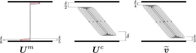
In this paper, we study equations (1.1a-b) within a Couette flow configuration (see Figure 1). One of the most important highlight of our work is the construction of a family of velocity fields $\{\boldsymbol{U}_{\nu}\}$ with almost anomalous dissipation, in particular the energy dissipation scales as ($(\log\nu^{-1})^{-2}$), such that the corresponding solutions $\{\boldsymbol{u}_{\nu}\}$ also has energy dissipation scaling at least as ($(\log\nu^{-1})^{-2}$). Notably, the rate of energy dissipation in both $\{\boldsymbol{U}_{\nu}\}$ and $\{\boldsymbol{u}_{\nu}\}$ is slower than power law $\nu^{\alpha}$ for any $\alpha>0$. Our result is sharp in the sense that a logarithmic decrease of energy dissipation in a channel flow is a prediction of phenomenological theories of wall turbulence (Schlichting and Gersten,, 2016) and have been observed in experiments (Smits etย al.,, 2011; Marusic etย al.,, 2013) to an enormous degree. As a side note, we observe that anomalous dissipation in channel or pipe flow geometries should, in principle, be achievable when there is sufficient transversal flow toward the boundary. For instance, see the work of Nguyenย van Yen etย al., (2011) on dipole crashing into a wall in two dimensions.

1.1 Purpose of studying equation (1.1) and anomalous dissipation in a vector field

The main purpose of introducing equations (1.1a-b) in this paper is to discuss a problem pertaining to anomalous dissipation in a divergence-free velocity field. However, the significance of these equations extends far beyond this topic. For instance, questions related to nonuniqueness and loss of regularity in the Navierโ€“Stokes equations are among the most pressing concerns in mathematical fluid dynamics. Equations (1.1a-b) provide a valuable platform for studying these problems without the complications introduced by the nonlinear term in the Navierโ€“Stokes equations. At the same time, these equations still require us to confront the true nature of the pressure term, which is absent in the advection-diffusion of a scalar. Consequently, studying equations (1.1) can allow us to gain deeper insights into the role of pressure in incompressible fluid flows.

An important characteristics of turbulent flow is that the rate of energy dissipation $\varepsilon$ becomes independent of viscosity in the limit of vanishingly small viscosity (Sreenivasan,, 1998; Frisch,, 1995). Mathematically, it means that the solution of the Navierโ€“Stokes equations (1.3) obey

$\displaystyle\varepsilon\coloneqq\nu\langle|\nabla\boldsymbol{u}|^{2}\rangle\geq c>0,\quad\forall\nu>0,$ (1.5)

for some constant $c$. Here, the angle brackets denote the long-time volume average:

$\displaystyle\langle[\,\cdot\,]\rangle\coloneqq\limsup_{T\to\infty}\frac{1}{T}\int_{0}^{T}\mathchoice{{\vbox{\hbox{$\textstyle-$ }}\kern-7.83337pt}}{{\vbox{\hbox{$\scriptstyle-$ }}\kern-5.90005pt}}{{\vbox{\hbox{$\scriptscriptstyle-$ }}\kern-4.75003pt}}{{\vbox{\hbox{$\scriptscriptstyle-$ }}\kern-4.25003pt}}\!\int_{\Omega}[\,\cdot\,]\,{\rm d}\boldsymbol{x}\,{\rm d}t,\qquad\text{where}\qquad\mathchoice{{\vbox{\hbox{$\textstyle-$ }}\kern-7.83337pt}}{{\vbox{\hbox{$\scriptstyle-$ }}\kern-5.90005pt}}{{\vbox{\hbox{$\scriptscriptstyle-$ }}\kern-4.75003pt}}{{\vbox{\hbox{$\scriptscriptstyle-$ }}\kern-4.25003pt}}\!\int_{\Omega}[\,\cdot\,]\,{\rm d}\boldsymbol{x}\coloneqq\frac{1}{|\Omega|}\int_{\Omega}[\,\cdot\,]\,{\rm d}\boldsymbol{x}.$ (1.6)

This phenomenon, known as the anomalous dissipation of energy and sometimes also referred to as the โ€œzeroth lawโ€ of turbulence due to its fundamental nature (Sreenivasan,, 1984). This phenomenon has been extensively validated through numerous experiments and direct numerical simulations (Pearson etย al.,, 2002; Kaneda etย al.,, 2003).

The phenomenon of anomalous dissipation can initially seem counterintuitive: how can a system continue to dissipate energy at a constant rate if the factor responsible for friction (in our case it would be viscosity) is gradually eliminated? For instance, in a rigid body system with finite number of degree of freedoms, such as a double pendulum, the rate of energy dissipation decreases linearly with the friction factor and eventually approaches zero. However, this analogy is not applicable for fluid systems, where the number of degrees of freedom can increase without bound as viscosity approaches zero. The turbulent flows acquire these increase number of degree of freedom through the increase in the number of small scales in the flow. The increase in small scales is responsible for the growth of $\langle|\nabla\boldsymbol{u}|^{2}\rangle$ and for turbulent flows this quantity grows precisely as $\nu^{-1}$ leading to anomalous dissipation of the energy.

Assuming that the turbulent flows acquires many of its mean properties through invariant solutions (steady or time-periodic) to the Navierโ€“Stokes equations (Kawahara etย al.,, 2012), one would expect to find a family of these simple invariant solutions that also exhibit anomalous dissipation. This raises the following question:

Question 1.1 (Solution of NSE with anomalous dissipation).

Is there a family of solution $\{\boldsymbol{u}_{\nu}\}_{\nu>0}$ to the Navierโ€“Stokes equations (1.3) for which

$\displaystyle\nu\langle|\nabla\boldsymbol{u}_{\nu}|^{2}\rangle\geq c>0\quad\text{for all}\quad\nu>0?$ (1.7)

Interestingly, to date, there are no known examplesโ€”whether steady or time-dependentโ€”flows that follow the relation (1.7) (Drivas,, 2022). The two physically motivated settings to consider this question are the following:

  1. (i)

    Tangential velocity-driven flow: In this setting $\Omega$ is a smooth domain with impermeable boundaries, where the flow is driven by a prescribed tangential boundary condition (independent of viscosity).

  2. (ii)

    Smooth body forcing-driven flow: The flow inside a periodic domain or a smooth bounded domain with homogeneous Dirichlet boundary condition driven by the presence of a smooth forcing $\boldsymbol{f}$ (independent of viscosity) in the equation (1.1 b). In this context, the quantity that is expected to become independent of viscosity is the energy dissipation per unit kinetic energy, i.e., $\frac{\nu\langle|\nabla\boldsymbol{u}_{\nu}|^{2}\rangle}{\langle|\boldsymbol{u}_{\nu}|^{2}\rangle}$.

We note that recently Bruรจ and De Lellis, (2023) considered the case where the forcing is allowed to depend on $\nu$. Constructing velocity fields that answers the Question 1.1 in the two settings mentioned above at present remains out of reach. Inspired by this question, one can pose a similar question within the framework of passive vector equation (1.1).

Question 1.2 (Anomalous dissipation in a divergence-free passive vector field).

For some $\nu_{0}>0$, can one construct a family of smooth divergence-free vector fields $\{\boldsymbol{U}_{\nu}\}_{\nu_{0}>\nu>0}$ exhibiting anomalous dissipation, in particular, obeying

$\displaystyle\lim_{\nu\to 0}\nu\langle|\nabla\boldsymbol{U}_{\nu}|^{2}\rangle=c_{1}>0$ (1.8)

such that the corresponding family of solutions $\{\boldsymbol{u}_{\nu}\}_{\nu_{0}>\nu>0}$ to (1.1) satisfies

$\displaystyle\nu\langle|\nabla\boldsymbol{u}_{\nu}|^{2}\rangle\geq c_{2}>0\quad\text{for all}\quad\nu\in(0,\nu_{0}).$ (1.9)

At first glance, it might appear that answering this question shouldnโ€™t be too difficult: if the advecting velocity field $\{\boldsymbol{U}_{\nu}\}_{\nu>0}$ exhibits anomalous dissipation, then it is plausible that the velocity field it transports, $\{\boldsymbol{u}_{\nu}\}_{\nu>0}$, should also display anomalous dissipation. For examples, if one creates small scale in the velocity field $\{\boldsymbol{U}_{\nu}\}_{\nu>0}$, one may expect that the transported field will also develop small scales. This logic holds true for a passive scalar, where the scalar obediently follows the Lagrangian paths of the velocity field $\boldsymbol{U}$. However, in the passive vector case, the introduction of pressure complicates matters and may resist the formation of small-scale structures if the velocity field $\boldsymbol{U}$ is not carefully designed. This makes addressing Question 1.2 more challenging compared to its counterpart concerning anomalous dissipation in a passive scalar. Therefore, before addressing the difficult Question 1.2 about anomalous dissipation in a passive vector field, one can ask a similar question about enhanced dissipation.

1.2 Enhanced dissipation in a vector field

Enhanced dissipation refers to a phenomenon where mixing, transport of scalar and momentum, or energy dissipation in a fluid occurs at a much faster rate compared to pure molecular diffusion (Cotiย Zelati etย al.,, 2020). This phenomenon has been widely studied recently in the mathematical fluid dynamics community. In a pure diffusion case, the rate of energy dissipation typically scales linearly with viscosity $\nu$ for small viscosity values. However, in the enhanced dissipation scenario, the rate of energy dissipation increases and potentially follow a mixed of power-law and logarithmic scaling $\nu^{\alpha}(\log\nu^{-1})^{\beta}$, where

$\displaystyle\alpha\in[0,1)\text{ and }\beta\in\mathbb{R}\text{ if }\alpha>0\text{ and }\beta\leq 0\text{ if }\alpha=0.$ (1.10)

With $\alpha=\beta=0$, we arrive at anomalous dissipation. In the context of passive vector equations (1.1), one can ask if the underlying advecting velocity field $\boldsymbol{U}$ is dissipation-enhancing, does that also mean the same is true for the advected velocity field $\boldsymbol{u}$? More precisely, we ask the following question.

Question 1.3 (Enhanced dissipation in a divergence-free vector field).

Given the admissible choices of constants $\alpha$ and $\beta$ as in (1.10), can one design smooth divergence-free vector fields $\{\boldsymbol{U}_{\nu}\}_{\nu_{0}>\nu>0}$ obeying

$\displaystyle\nu\langle|\nabla\boldsymbol{U}_{\nu}|^{2}\rangle\sim\nu^{\alpha}(\log\nu^{-1})^{\beta},$ (1.11)

such that the corresponding family of solutions $\{\boldsymbol{u}_{\nu}\}_{\nu_{0}>\nu>0}$ to (1.1) satisfies

$\displaystyle\nu\langle|\nabla\boldsymbol{u}_{\nu}|^{2}\rangle\geq c\nu^{\alpha}(\log\nu^{-1})^{\beta}\quad\text{for all}\quad\nu\in(0,\nu_{0}),$ (1.12)

where $c>0$ is some constant?

In this paper, we answer this question affirmative with $\alpha=0$ and $\beta=-2$ in a Couette flow system. Therefore, both the advecting velocity fields $\{\boldsymbol{U}_{\nu}\}$ and passive velocity fields $\{\boldsymbol{u}_{\nu}\}$ are anomalous dissipating and only miss by a factor of logarithm.

1.3 Couette Flow

In this paper, we focus on the well-known Couette flow configuration, which serves as a paradigmatic system for studying turbulence within a shear layer. It is arguably one of the most extensively studied flow configurations due to its simple geometry, which facilitates both experimental design and direct numerical simulations. The Couette flow is the flow of fluid between two parallel plates, where the bottom plate is stationary and to top plate moves with a prescribed velocity. We solve the equations (1.1a-b) in the domain

$\displaystyle\Omega\coloneqq\mathbb{T}_{L_{1}}\times[-1/2,1/2]\times\mathbb{T}_{L_{3}}.$ (1.13)
Refer to caption
Figure 1: shows the schematic of the flow configuration.

Figure 1 shows a schematic of the flow configuration. We employ a Cartesian coordinate system $(x_{1},x_{2},x_{3})$, where $x_{1}$ and $x_{3}$ represent the periodic direction directions with length $L_{1}$ and $L_{3}$ respectively, while $x_{2}$ denotes the wall-normal direction. The velocity field $\boldsymbol{u}$ and $\boldsymbol{U}$ satisfy the same initial conditions:

$\displaystyle\boldsymbol{U}(t,\cdot)\to\boldsymbol{u}_{0},\quad\boldsymbol{u}(t,\cdot)\to\boldsymbol{u}_{0}\qquad\text{in }L^{2}(\Omega)\text{ as }t\to 0^{+},$ (1.14)

and boundary conditions:

$\displaystyle\boldsymbol{U}(t,x_{1},-1/2,x_{3})=\boldsymbol{u}(t,x_{1},-1/2,x_{3})=-\boldsymbol{e}_{1}/2\qquad\boldsymbol{U}(t,x_{1},1/2,x_{3})=\boldsymbol{u}(t,x_{1},1/2,x_{3})=\boldsymbol{e}_{1}/2,$ (1.15)

for all $t>0$ and $(x_{1},x_{3})\in\mathbb{T}_{L_{1}}\times\mathbb{T}_{L_{3}}$, where $\boldsymbol{e}_{1}$ is the unit vector in the $x_{1}$ direction.

In rest of the paper, we will consider that the velocity field $\boldsymbol{U}$ belongs to $L^{2}([0,\infty);H^{1}(\Omega))\cap L^{\infty}([0,\infty)\times\Omega)$. Furthermore, we assume that $\boldsymbol{u}_{0}\in H^{1}(\Omega)$. Therefore, there is a unique solution $\boldsymbol{u}\in L^{\infty}([0,\infty);H^{1}(\Omega))\cap L^{2}([0,\infty);H^{2}(\Omega))$ of the equations (1.1a-b) with initial condition (1.14) and boundary conditions (1.15).

Next, we define

$\displaystyle\varepsilon_{\boldsymbol{U}}\coloneq\nu\langle|\nabla\boldsymbol{U}|^{2}\rangle,\qquad\qquad\varepsilon_{\boldsymbol{u}}\coloneq\nu\langle|\nabla\boldsymbol{u}|^{2}\rangle$ (1.16)

to be the energy dissipation in the velocity $\boldsymbol{U}$ and $\boldsymbol{u}$ respectively. Recall, the angle brackets denote the long-time volume average as defined in (1.17). For convenience, we also define the long-time horizontal average, which we denote using overbar, as

$\displaystyle\overline{[\,\cdot\,]}\coloneqq\limsup_{T\to\infty}\frac{1}{T}\int_{0}^{T}\mathchoice{{\vbox{\hbox{$\textstyle-$ }}\kern-7.83337pt}}{{\vbox{\hbox{$\scriptstyle-$ }}\kern-5.90005pt}}{{\vbox{\hbox{$\scriptscriptstyle-$ }}\kern-4.75003pt}}{{\vbox{\hbox{$\scriptscriptstyle-$ }}\kern-4.25003pt}}\!\int_{\mathbb{T}_{L_{1}}\times\mathbb{T}_{L_{3}}}[\,\cdot\,]\,{\rm d}\boldsymbol{s}\,{\rm d}t\qquad\text{and}\qquad\mathchoice{{\vbox{\hbox{$\textstyle-$ }}\kern-7.83337pt}}{{\vbox{\hbox{$\scriptstyle-$ }}\kern-5.90005pt}}{{\vbox{\hbox{$\scriptscriptstyle-$ }}\kern-4.75003pt}}{{\vbox{\hbox{$\scriptscriptstyle-$ }}\kern-4.25003pt}}\!\int_{\mathbb{T}_{L_{1}}\times\mathbb{T}_{L_{3}}}[\,\cdot\,]\,{\rm d}\boldsymbol{s}\coloneqq\frac{1}{L_{1}\,L_{3}}\int_{\Omega}[\,\cdot\,]\,{\rm d}x_{1}{\rm d}x_{3}.$ (1.17)

Next, we state the main results of our paper, all of which are in the Couette flow setting. The first result provides an upper bound on the dissipation in $\boldsymbol{u}$ in terms of the dissipation in $\boldsymbol{U}$.

Theorem 1.4 (Main result I: Upper bound).

Let the energy dissipation in $\boldsymbol{U}$ and $\boldsymbol{u}$ be given by (1.16). Then we have the following upper bound

$\displaystyle\varepsilon_{\boldsymbol{u}}\leq 4(\varepsilon_{\boldsymbol{U}})^{\frac{1}{3}}.$ (1.18)

Therefore, if $\{\boldsymbol{U}_{\nu}\}_{\nu>0}$, a family of divergence-free velocity fields, obeys $\nu\langle|\nabla\boldsymbol{U}_{\nu}|^{2}\rangle\sim\nu^{\alpha}(\log\nu^{-1})^{\beta}$ then the corresponding solutions $\{\boldsymbol{u}_{\nu}\}_{\nu>0}$ to equations (1.1a-b) will obey $\nu\langle|\nabla\boldsymbol{u}_{\nu}|^{2}\rangle\leq c\nu^{\frac{\alpha}{3}}(\log\nu^{-1})^{\frac{\beta}{3}}$ for some positive constant $c$.

Our second result is a construction, we prove the following:

Theorem 1.5 (Main result II: Construction).

There exists a family of smooth divergence-free velocity field $\{\boldsymbol{U}_{\nu}\}_{0<\nu<1/500}$ with $\nu\langle|\nabla\boldsymbol{U}_{\nu}|^{2}\rangle\sim(\log(\nu^{-1}))^{2}$ such that the solutions to equations (1.1a-b) satisfy $\nu\langle|\nabla\boldsymbol{u}_{\nu}|^{2}\rangle\geq c(\log(\nu^{-1}))^{2}$.

Remark 1.1.

The proof of Theorem 1.4 relies on the method by Seis, (2015). The result for values other than $\alpha=0$ and $\beta=0$ may not be sharp as it does not seem physical for the advected velocity field $\boldsymbol{u}$ to be dissipating more energy than the advecting velocity field $\boldsymbol{U}$. This raises the following question:

Question 1.6 (Improved upper bound).

If $\{\boldsymbol{U}_{\nu}\}_{\nu>0}$ obeys $\nu\langle|\nabla\boldsymbol{U}_{\nu}|^{2}\rangle\sim\nu^{\alpha}(\log\nu)^{\beta}$ with $\alpha$ and $\beta$ as given in (1.10) then is it true that the corresponding solutions $\{\boldsymbol{u}_{\nu}\}_{\nu>0}$ to equations (1.1a-b) will obey $\nu\langle|\nabla\boldsymbol{u}_{\nu}|^{2}\rangle\leq c\nu^{\alpha}(\log\nu)^{\beta}$ for some positive constant $c$?

The proof of Theorem 1.5 is based on a variational principle for the energy dissipation rate in the velocity field $\boldsymbol{u}$ derived in Section 3, which is similar to variational approaches recently used in the context of advection-diffusion in a scalar for problems related to optimal heat transport (Doering and Tobasco,, 2019; Kumar,, 2022). The main idea is to use a branching flow construction to a give a proof of Theorem 1.5. However, we also provide a subptimal answer to Question 1.3 using a construction based on convection rolls with $\alpha=1/3$ and $\beta=0$. This construction serves a dual purpose: it demonstrates the application of the variational principle (before going to the more complex branching flow construction) and is also physically motivated, as convection rolls are commonly observed in fluid dynamics and are effective in heat and momentum transfer. Consequently, this work may inspire further research into finding exact solutions of the Navierโ€“Stokes equations based on convection rolls in a Couette flow configuration, both from mathematical analysis and computational side, as the convection rolls seem more tractable than the branching flows.

1.4 Comparison with experiments and numerical observation

The single most important aspect of our result in Theorem 1.5 is that the energy dissipation scaling $(\log\nu^{-1})^{-2}$ is the predictions from the prominent phenomenological theories of turbulent channel flow (or wall-bounded turbulence in general) and has been validated in experiments to a considerable degree. From the vast literature on this subject, we note only the most important references (Schlichting and Gersten,, 2016; Smits etย al.,, 2011; Yakhot etย al.,, 2010; Marusic etย al.,, 2010). Beyond the statistical property, our flow design in Theorem 1.5 shares several structural similarities. We illuminate on these two features in the paragraphs below.

The near anomalous dissipation scaling of the energy dissipation in a channel flow is a prediction of the so-called โ€œlaw of the wallโ€ or โ€œlogarithmic law.โ€ This law asserts that the mean velocity of the flow near the wall scales logarithmically with the distance from the wall, a characteristic behavior observed in turbulent flows. It describes three distinct layers in turbulent flow: (i) the viscous layer (closest to the wall), (ii) the outer layer (further away from the wall), and (iii) the overlap layer. In the viscous layer, viscous effects dominate, and the velocity profile in this region is independent of the channel height. In the outer layer, the velocity is influenced only by the channel height and does not account for viscosity. Finally, in the overlap region, the velocity is independent of both viscosity and channel height, leading to a logarithmic velocity profile. A consequence of this logarithmic profile is that the energy dissipation scales as

$\displaystyle\nu\langle|\nabla\boldsymbol{u}|^{2}\rangle\sim\frac{1}{4}\frac{\kappa^{2}}{(\log\nu^{-1})^{2}}\approx\frac{0.042}{(\log\nu^{-1})^{2}},$ (1.19)

where $\kappa\approx 0.41$ is know as the โ€œvon Kรกrmรกnโ€ constant, a universal constant in wall-bounded turbulent flows (Schlichting and Gersten,, 2016). We caution the reader that the result in (1.19) is often stated in the engineering and physics literature in terms of the friction factor (which is related to energy dissipation) and the Reynolds number $Re=\nu^{-1}U_{c}H$, where $U_{c}$ is the velocity of the walls ($1/2$ in our case) and $H$ is the half channel width (also $1/2$ in our case).

The second aspect we wish to emphasize regarding our flow design in Theorem 1.5 is the self-similar nature of the construction, which is characterized by overlapping eddies and is crucial for achieving the logarithmic decay of energy dissipation. We note that the self-similar hierarchical structure is also prevalent in wall turbulence. In a seminal work, Townsend hypothesized that the flow within the log layer comprises a self-similar population of eddies of varying sizes that are attached to the wall (Townsend,, 1976). Such structures have been observed in direct numerical simulations (DNS) (Lozano-Durรกn etย al.,, 2012; Hwang,, 2015), numerically constructed invariant solutions (Yang etย al.,, 2019), resolvent analysis (McKeon,, 2019), and proper orthogonal decomposition of data from pipe flow (Hellstrรถm etย al.,, 2016). Given the scaling results of our velocity field construction and the similarity in flow structures, it is evident that our construction is closely related to physically observed flows and is not merely a mathematical construct.

1.5 Organization of the paper

In Section 2, we provide a proof of Theorem 1.4 by establishing an upper bound on the energy dissipation. Section 3 is dedicated to deriving a variational principle for the rate of energy dissipation. We present a construction based on convection rolls in Section 4. Next, we prove Theorem 1.5 in Section 5, which relies on branching flows. Finally, we conclude with a discussion and future outlook in Section 6.

Acknowledgement

A.K. thanks Sergei Chernyshenko for insightful discussions on the law of the wall. A.K. also thanks Theodore Drivas and Vlad Vicol for valuable suggestions.

2 Upper Bound

As the velocity field $\boldsymbol{U}\in L^{2}([0,\infty);H^{1}(\Omega))\cap L^{\infty}([0,\infty)\times\Omega)$. Therefore, there is a unique strong solution $\boldsymbol{u}$ of the equations (1.1a-b). Taking the dot product of equation (1.1b) with $\boldsymbol{u}$ then gives

$\displaystyle\frac{1}{2}\partial_{t}|\boldsymbol{u}|^{2}+\frac{1}{2}\mathop{div}\nolimits(\boldsymbol{U}|\boldsymbol{u}|^{2})=-\mathop{div}\nolimits(\boldsymbol{u}p)+\nu\sum_{i,j}\partial_{j}(u_{i}\partial_{j}u_{i})-\nu|\nabla\boldsymbol{u}|^{2}.$ (2.1)

Taking a volume average of above equation leads to

$\displaystyle\frac{1}{2}\frac{d}{dt}\mathchoice{{\vbox{\hbox{$\textstyle-$ }}\kern-7.83337pt}}{{\vbox{\hbox{$\scriptstyle-$ }}\kern-5.90005pt}}{{\vbox{\hbox{$\scriptscriptstyle-$ }}\kern-4.75003pt}}{{\vbox{\hbox{$\scriptscriptstyle-$ }}\kern-4.25003pt}}\!\int_{\Omega}|\boldsymbol{u}|^{2}\,{\rm d}\boldsymbol{x}=\frac{\nu}{2}\mathchoice{{\vbox{\hbox{$\textstyle-$ }}\kern-7.83337pt}}{{\vbox{\hbox{$\scriptstyle-$ }}\kern-5.90005pt}}{{\vbox{\hbox{$\scriptscriptstyle-$ }}\kern-4.75003pt}}{{\vbox{\hbox{$\scriptscriptstyle-$ }}\kern-4.25003pt}}\!\int_{\mathbb{T}_{L_{x}}\times\mathbb{T}_{L_{y}}}\left[\left.\partial_{2}u_{1}\right|_{x_{2}=1/2}+\left.\partial_{2}u_{1}\right|_{x_{2}=-1/2}\right]{\rm d}\boldsymbol{s}-\nu\mathchoice{{\vbox{\hbox{$\textstyle-$ }}\kern-7.83337pt}}{{\vbox{\hbox{$\scriptstyle-$ }}\kern-5.90005pt}}{{\vbox{\hbox{$\scriptscriptstyle-$ }}\kern-4.75003pt}}{{\vbox{\hbox{$\scriptscriptstyle-$ }}\kern-4.25003pt}}\!\int_{\Omega}|\nabla\boldsymbol{u}|^{2}\,{\rm d}\boldsymbol{x}.$ (2.2)

Finally, noting that $\boldsymbol{u}\in L^{\infty}([0,\infty);L^{2}(\Omega))$, performing a long-time average leads to

$\displaystyle\nu\langle|\nabla\boldsymbol{u}|^{2}\rangle=\frac{\nu}{2}\overline{\left.\partial_{2}u_{1}\right|_{x_{2}=1/2}}+\frac{\nu}{2}\overline{\left.\partial_{2}u_{1}\right|_{x_{2}=-1/2}}.$ (2.3)

By performing the long-time horizontal average of the $x_{1}$ component of equation (1.1b) at any level $x_{2}$ gives

ฮฝโ€‹โˆ‚2u1ยฏโˆ’U2โ€‹u1ยฏ=cโ€‹oโ€‹nโ€‹sโ€‹tfor allย โ€‹x2โˆˆ[โˆ’1/2,1/2].formulae-sequence๐œˆยฏsubscript2subscript๐‘ข1ยฏsubscript๐‘ˆ2subscript๐‘ข1๐‘๐‘œ๐‘›๐‘ ๐‘กfor allย subscript๐‘ฅ21212\displaystyle\nu\overline{\partial_{2}u_{1}}-\overline{U_{2}u_{1}}=const\quad\text{for all }x_{2}\in[-1/2,1/2]. (2.4)

Combining (2.3) and (2.4), we get

$\displaystyle\nu\langle|\nabla\boldsymbol{u}|^{2}\rangle=\nu\overline{\partial_{2}u_{1}}-\overline{U_{2}u_{1}}\quad\text{for all }x_{2}\in[-1/2,1/2].$ (2.5)

Therefore, the equality also holds when the right-hand side in (2.5) is replaced by its average over the layer

$$\Gamma_{\delta}\coloneqq[-1/2,-1/2+\delta]$$

of thickness $\delta$ near the bottom wall leading to

$\displaystyle\nu\langle|\nabla\boldsymbol{u}|^{2}\rangle$ $\displaystyle=\nu\overline{\mathchoice{{\vbox{\hbox{$\textstyle-$ }}\kern-7.83337pt}}{{\vbox{\hbox{$\scriptstyle-$ }}\kern-5.90005pt}}{{\vbox{\hbox{$\scriptscriptstyle-$ }}\kern-4.75003pt}}{{\vbox{\hbox{$\scriptscriptstyle-$ }}\kern-4.25003pt}}\!\int_{\Gamma_{\delta}}\partial_{2}u_{1}}-\overline{\mathchoice{{\vbox{\hbox{$\textstyle-$ }}\kern-7.83337pt}}{{\vbox{\hbox{$\scriptstyle-$ }}\kern-5.90005pt}}{{\vbox{\hbox{$\scriptscriptstyle-$ }}\kern-4.75003pt}}{{\vbox{\hbox{$\scriptscriptstyle-$ }}\kern-4.25003pt}}\!\int_{\Gamma_{\delta}}U_{2}u_{1}}\qquad\text{where}\quad\mathchoice{{\vbox{\hbox{$\textstyle-$ }}\kern-7.83337pt}}{{\vbox{\hbox{$\scriptstyle-$ }}\kern-5.90005pt}}{{\vbox{\hbox{$\scriptscriptstyle-$ }}\kern-4.75003pt}}{{\vbox{\hbox{$\scriptscriptstyle-$ }}\kern-4.25003pt}}\!\int_{\Gamma_{\delta}}[\,\cdot\,]\coloneqq\frac{1}{\delta}\int_{x_{2}\in\Gamma_{\delta}}[\,\cdot\,]\,{\rm}dx_{2}.$ (2.6)

Next, we have the following estimate:

$\displaystyle\left|\,\overline{\mathchoice{{\vbox{\hbox{$\textstyle-$ }}\kern-7.83337pt}}{{\vbox{\hbox{$\scriptstyle-$ }}\kern-5.90005pt}}{{\vbox{\hbox{$\scriptscriptstyle-$ }}\kern-4.75003pt}}{{\vbox{\hbox{$\scriptscriptstyle-$ }}\kern-4.25003pt}}\!\int_{\Gamma_{\delta}}\partial_{2}u_{1}}\,\right|\leq\left(\,\overline{\mathchoice{{\vbox{\hbox{$\textstyle-$ }}\kern-7.83337pt}}{{\vbox{\hbox{$\scriptstyle-$ }}\kern-5.90005pt}}{{\vbox{\hbox{$\scriptscriptstyle-$ }}\kern-4.75003pt}}{{\vbox{\hbox{$\scriptscriptstyle-$ }}\kern-4.25003pt}}\!\int_{\Gamma_{\delta}}(\partial_{2}u_{1})^{2}}\,\right)^{\frac{1}{2}}\leq\nu^{-1/2}\delta^{-1/2}(\varepsilon_{\boldsymbol{u}})^{\frac{1}{2}}.$ (2.7)

We also have

$\displaystyle\left|\overline{\mathchoice{{\vbox{\hbox{$\textstyle-$ }}\kern-7.83337pt}}{{\vbox{\hbox{$\scriptstyle-$ }}\kern-5.90005pt}}{{\vbox{\hbox{$\scriptscriptstyle-$ }}\kern-4.75003pt}}{{\vbox{\hbox{$\scriptscriptstyle-$ }}\kern-4.25003pt}}\!\int_{\Gamma_{\delta}}U_{2}u_{1}}\right|$ $\displaystyle\leq\left(\,\overline{\mathchoice{{\vbox{\hbox{$\textstyle-$ }}\kern-7.83337pt}}{{\vbox{\hbox{$\scriptstyle-$ }}\kern-5.90005pt}}{{\vbox{\hbox{$\scriptscriptstyle-$ }}\kern-4.75003pt}}{{\vbox{\hbox{$\scriptscriptstyle-$ }}\kern-4.25003pt}}\!\int_{\Gamma_{\delta}}U_{2}^{2}}\,\right)^{\frac{1}{2}}\left(\,\overline{\mathchoice{{\vbox{\hbox{$\textstyle-$ }}\kern-7.83337pt}}{{\vbox{\hbox{$\scriptstyle-$ }}\kern-5.90005pt}}{{\vbox{\hbox{$\scriptscriptstyle-$ }}\kern-4.75003pt}}{{\vbox{\hbox{$\scriptscriptstyle-$ }}\kern-4.25003pt}}\!\int_{\Gamma_{\delta}}u_{1}^{2}}\,\right)^{\frac{1}{2}}$
$\displaystyle\leq\delta^{2}\left(\,\overline{\mathchoice{{\vbox{\hbox{$\textstyle-$ }}\kern-7.83337pt}}{{\vbox{\hbox{$\scriptstyle-$ }}\kern-5.90005pt}}{{\vbox{\hbox{$\scriptscriptstyle-$ }}\kern-4.75003pt}}{{\vbox{\hbox{$\scriptscriptstyle-$ }}\kern-4.25003pt}}\!\int_{\Gamma_{\delta}}(\partial_{2}U_{2})^{2}\,}\right)^{\frac{1}{2}}\left(\,\overline{\mathchoice{{\vbox{\hbox{$\textstyle-$ }}\kern-7.83337pt}}{{\vbox{\hbox{$\scriptstyle-$ }}\kern-5.90005pt}}{{\vbox{\hbox{$\scriptscriptstyle-$ }}\kern-4.75003pt}}{{\vbox{\hbox{$\scriptscriptstyle-$ }}\kern-4.25003pt}}\!\int_{\Gamma_{\delta}}(\partial_{2}u_{1})^{2}}\,\right)^{\frac{1}{2}}$
$\displaystyle\leq\delta\nu^{-1}(\varepsilon_{\boldsymbol{U}})^{\frac{1}{2}}(\varepsilon_{\boldsymbol{u}})^{\frac{1}{2}}.$ (2.8)

Combining (2.6) with (2.7) and (2.8) leads to

$\displaystyle\varepsilon_{\boldsymbol{u}}\leq\nu^{1/2}\delta^{-1/2}(\varepsilon_{\boldsymbol{u}})^{\frac{1}{2}}+\delta\nu^{-1}(\varepsilon_{\boldsymbol{U}})^{\frac{1}{2}}(\varepsilon_{\boldsymbol{u}})^{\frac{1}{2}}$
$\displaystyle\implies$ $\displaystyle\varepsilon_{\boldsymbol{u}}\leq\left(\nu^{1/2}\delta^{-1/2}+\delta\nu^{-1}(\varepsilon_{\boldsymbol{U}})^{\frac{1}{2}}\right)^{2}.$ (2.9)

Finally, selecting

$$\delta=\frac{\nu}{(\varepsilon_{\boldsymbol{U}})^{\frac{1}{3}}}$$

gives

$\displaystyle\varepsilon_{\boldsymbol{u}}\leq 4(\varepsilon_{\boldsymbol{U}})^{\frac{1}{3}}.$ (2.10)

3 Variational principle for the energy dissipation rate

To prove Theorem 1.5, we will design a family of time-independent divergence-free velocity field $\{\boldsymbol{U}_{\nu}\}_{\nu>0}$. As a result, in long-time averages of the solutions of (1.1), any dependence on the initial data $\boldsymbol{u}_{0}$ is ultimately lost, and the long-time averages depend solely on the solutions of the corresponding steady equations:

$\displaystyle\nabla\cdot\boldsymbol{u}=0,$ (3.1a)
$\displaystyle\boldsymbol{U}\cdot\nabla\boldsymbol{u}=-\nabla p+\nu\Delta\boldsymbol{u}.$ (3.1b)

When the choice of $\boldsymbol{U}$ involves a combination of translation and rigid body motion, the resulting equations are known as Oseenโ€™s equations (Galdi,, 2011). However, in our study, we do not limit $\boldsymbol{U}$ to just these two forms. The construction that follows in the next two sections, the design of the velocity fields $\{\boldsymbol{U}_{\nu}\}_{\nu>0}$ is two dimensional. Because of this simplification, from here onward, without loss of generality, our domain will be

$\displaystyle\Omega=\mathbb{T}_{L_{1}}\times[-1/2,1/2],$ (3.2)

and the angle brackets will only mean the volume averages

$\displaystyle\langle[\,\cdot\,]\rangle=\mathchoice{{\vbox{\hbox{$\textstyle-$ }}\kern-7.83337pt}}{{\vbox{\hbox{$\scriptstyle-$ }}\kern-5.90005pt}}{{\vbox{\hbox{$\scriptscriptstyle-$ }}\kern-4.75003pt}}{{\vbox{\hbox{$\scriptscriptstyle-$ }}\kern-4.25003pt}}\!\int_{\Omega}[\,\cdot\,]\,{\rm d}\boldsymbol{x}.$ (3.3)

The velocity fields $\boldsymbol{U}$ and $\boldsymbol{u}$ satisfy the same boundary conditions on the top and bottom walls

$\displaystyle\boldsymbol{U}(x_{1},-1/2)=\boldsymbol{u}(x_{1},-1/2)=-\boldsymbol{e}_{1}/2,\qquad\boldsymbol{U}(x_{1},1/2)=\boldsymbol{u}(x_{1},1/2)=\boldsymbol{e}_{1}/2,$ (3.4)

for all $x_{1}\in\mathbb{T}_{L_{1}}$.

Remark 3.1.

From the broader perspective of the time-dependent advection-diffusion equation, the velocity field $\boldsymbol{U}$ may not initially satisfy the given conditions. To resolve this discrepancy, the velocity field $\boldsymbol{U}$ is designed to smoothly transition from the initial condition over the first unit of time. After this initial period, $\boldsymbol{U}$ assumes the desired autonomous form.

We assume in rest of the section we assume that $\boldsymbol{U}\in L^{\infty}(\Omega)$. Therefore, there is a unique weak solution $\boldsymbol{u}\in H^{1}(\Omega)$ to (3.1) satisfying the boundary conditions (3.4). Also, we denote the Leary projector by $\mathbb{P}$ and the $\Delta^{-1}$ to be the inverse Laplace operator with respect to homogeneous boundary conditions on the walls $x_{2}=\pm\frac{1}{2}$.

Proposition 3.1 (Variational principle for energy dissipation rate).

Let $\boldsymbol{U}\in L^{\infty}(\Omega)$ be a weakly divergence-free vector field. Then the energy dissipation in the solution $\boldsymbol{u}$ of (3.1) satisfies

$\displaystyle\nu\langle|\nabla\boldsymbol{u}|^{2}\rangle-\nu=\max_{\begin{subarray}{c}\widetilde{\boldsymbol{v}}\in H^{1}_{0}(\Omega)\\ \mathop{div}\nolimits\widetilde{\boldsymbol{v}}=0\end{subarray}}\left(-2\langle U_{2}\widetilde{v}_{1}\rangle-\nu\langle|\nabla\widetilde{\boldsymbol{v}}|^{2}\rangle-\frac{1}{\nu}\langle|\nabla\Delta^{-1}\mathbb{P}\boldsymbol{U}\cdot\nabla\widetilde{\boldsymbol{v}}|^{2}\rangle\right).$ (3.5)
Proof.

We decompose the velocity field $\boldsymbol{u}$ into a linear part and a homogeneous part:

$\displaystyle\boldsymbol{u}=x_{2}\boldsymbol{e}_{1}+\boldsymbol{v}.$ (3.6)

Using (3.6) in (3.1) and (3.4), it is clear that $\boldsymbol{v}$ satisfies

$\displaystyle\nabla\cdot\boldsymbol{v}=0,$ (3.7a)
$\displaystyle U_{2}\boldsymbol{e}_{1}+\boldsymbol{U}\cdot\nabla\boldsymbol{v}=-\nabla p+\nu\Delta\boldsymbol{v}.$ (3.7b)

along with the homogeneous version of the boundary conditions. From the decomposition (3.6), we observe that

$\displaystyle\nu\langle|\nabla\boldsymbol{u}|^{2}\rangle=\nu\langle|\nabla\boldsymbol{v}|^{2}\rangle+\nu.$ (3.8)

Also, taking the dot product of (3.7b) with $\boldsymbol{v}$ and performing a volume average leads to

$\displaystyle\nu\langle|\nabla\boldsymbol{v}|^{2}\rangle=-\langle U_{2}v_{1}\rangle$ (3.9)

Therefore, we can also write

$\displaystyle\nu\langle|\nabla\boldsymbol{u}|^{2}\rangle=-\langle U_{2}v_{1}\rangle+\nu.$ (3.10)

Next, consider two sets of PDEs,

$\displaystyle\nabla\cdot\widetilde{\boldsymbol{v}}=0,$ (3.11a)
$\displaystyle U_{2}\boldsymbol{e}_{1}+\boldsymbol{U}\cdot\nabla\overline{\boldsymbol{v}}=-\nabla\widetilde{p}+\nu\Delta\widetilde{\boldsymbol{v}},$ (3.11b)

and

$\displaystyle\nabla\cdot\overline{\boldsymbol{v}}=0,$ (3.12a)
$\displaystyle\boldsymbol{U}\cdot\nabla\widetilde{\boldsymbol{v}}=-\nabla\overline{p}+\nu\Delta\overline{\boldsymbol{v}},$ (3.12b)

where $\overline{\boldsymbol{v}},\widetilde{\boldsymbol{v}}:\Omega\to\mathbb{R}^{2}$ satisfies the zero velocity boundary conditions, i.e.,

$\displaystyle\overline{\boldsymbol{v}},\;\widetilde{\boldsymbol{v}}=\boldsymbol{0},\qquad x_{2}=\pm\frac{1}{2}.$ (3.13)

This is a standard symmetrization procedure previously used in the studies of optimal heat transport (Doering and Tobasco,, 2019). Now, from the standard existence uniqueness theory, there are unique solutions $\widetilde{\boldsymbol{v}},\overline{\boldsymbol{v}}\in H^{1}_{0}(\Omega)$ to PDEs (3.11) and (3.12). Moreover, it is clear that we can write our solution $\boldsymbol{v}$ to equations (3.7) as

$\displaystyle\boldsymbol{v}=\overline{\boldsymbol{v}}+\widetilde{\boldsymbol{v}}.$ (3.14)

Taking the dot product of equation (3.12b) with $\widetilde{\boldsymbol{v}}$ leads to

$\displaystyle\langle\nabla\overline{\boldsymbol{v}}\colon\nabla\widetilde{\boldsymbol{v}}\rangle=0,$ (3.15)

where in the index notation, we have $\nabla\overline{\boldsymbol{v}}\colon\nabla\widetilde{\boldsymbol{v}}=\partial_{j}\overline{v}_{i}\partial_{j}\widetilde{v}_{i}$. Next, we take the dot product of the equation (3.11b) with $\overline{\boldsymbol{v}}$ and integrate which leads to

$\displaystyle\langle U_{2}\overline{v}_{1}\rangle=0.$ (3.16)

Substituting (3.14) in (3.8) and then using (3.15) leads to

$\displaystyle\nu\langle|\nabla\boldsymbol{u}|^{2}\rangle$ $\displaystyle=\nu\langle|\nabla\widetilde{\boldsymbol{v}}|^{2}\rangle+\nu\langle|\nabla\overline{\boldsymbol{v}}|^{2}\rangle+\nu$
$\displaystyle=\nu\langle|\nabla\widetilde{\boldsymbol{v}}|^{2}\rangle+\frac{1}{\nu}\langle|\nabla\Delta^{-1}\mathbb{P}\boldsymbol{U}\cdot\nabla\widetilde{\boldsymbol{v}}|^{2}\rangle+\nu.$ (3.17)

Using (3.16) in (3.10) gives

$\displaystyle\nu\langle|\nabla\boldsymbol{u}|^{2}\rangle=-\langle U_{2}\widetilde{v}_{1}\rangle+\nu.$ (3.18)

Finally, multiplying (3.18) with two and then subtracting (3.17) yields

$\displaystyle\nu\langle|\nabla\boldsymbol{u}|^{2}\rangle-\nu=F(\widetilde{\boldsymbol{v}}),$ (3.19)

where

$\displaystyle F(\widetilde{\boldsymbol{v}})\coloneqq-2\langle U_{2}\widetilde{v}_{1}\rangle-\nu\langle|\nabla\widetilde{\boldsymbol{v}}|^{2}\rangle-\frac{1}{\nu}\langle|\nabla\Delta^{-1}\mathbb{P}\boldsymbol{U}\cdot\nabla\widetilde{\boldsymbol{v}}|^{2}\rangle.$ (3.20)

Next, we consider the following variational problem:

$\displaystyle\sup_{\begin{subarray}{c}\widetilde{\boldsymbol{v}}\in H^{1}_{0}(\Omega)\\ \mathop{div}\nolimits\widetilde{\boldsymbol{v}}=0\end{subarray}}F(\widetilde{\boldsymbol{v}}).$ (3.21)

We see that $F$ is concave so it has a unique maximizer. Moreover, the maximizer $\widetilde{\boldsymbol{v}}$ solves the Eulerโ€“Lagrange equation

$\displaystyle U_{2}\boldsymbol{e}_{1}+\frac{1}{\nu}\boldsymbol{U}\cdot\nabla\Delta^{-1}(\mathbb{P}\boldsymbol{U}\cdot\nabla\widetilde{\boldsymbol{v}})=-\nabla q+\nu\Delta\widetilde{\boldsymbol{v}}$ (3.22)

which is basically the PDE (3.11b). Therefore, the variational principle (3.5) follows. Finally, note that one could have also used a method based on Lagrange multiplier to derive this variational principle. See, for example, (Song etย al.,, 2023) in the context of heat transfer. โˆŽ

4 Convection Rolls Based Design

In this section, we demonstrate the existence of a family of divergence-free velocity fields $\{\boldsymbol{U}_{\nu}\}_{\nu>0}$ with energy dissipation scaling as $\nu\langle|\nabla\boldsymbol{U}_{\nu}|^{2}\rangle\sim\nu^{1/3}$, such that for the corresponding passive vector fields, the energy dissipation scales at least as $\nu\langle|\nabla\boldsymbol{u}_{\nu}|^{2}\rangle\gtrsim\nu^{1/3}$. For brevity, we will omit $\nu$ from the subscript in the remainder of this section. The first step involves constructing a candidate for the convecting velocity field $\boldsymbol{U}$. Once $\boldsymbol{U}$ is constructed, we turn to the variational principle (3.5) derived in the previous section to obtain a bound on the energy dissipation in $\boldsymbol{u}$. Therefore, the second step consists of making a โ€˜good choiceโ€™ of the divergence-free test vector field $\widetilde{\boldsymbol{v}}\in H^{1}_{0}(\Omega)$, which then provides the following bound

$\displaystyle\nu\langle|\nabla\boldsymbol{u}|^{2}\rangle-\nu\geq I+II+III,$ (4.1)

where

$\displaystyle I\coloneqq-2\langle U_{2}\widetilde{v}_{1}\rangle,\qquad II\coloneqq-\nu\langle|\nabla\widetilde{\boldsymbol{v}}|^{2}\rangle,\qquad III\coloneqq-\frac{1}{\nu}\langle|\nabla\Delta^{-1}\mathbb{P}\boldsymbol{U}\cdot\nabla\widetilde{\boldsymbol{v}}|^{2}\rangle.$ (4.2)

Finally, the last task is to estimate all the terms $I$, $II$ and $III$.

4.1 Choice of the velocity field $\boldsymbol{U}$

Our choice of the velocity field $\boldsymbol{U}$ is the sum of two divergence-free velocity fields:

$\displaystyle\boldsymbol{U}=\boldsymbol{U}^{m}+\boldsymbol{U}^{c}.$ (4.3)

The velocity field $\boldsymbol{U}^{m}$ is a unidirectional flow in the $x_{1}$ direction that satisfies the same boundary conditions as $\boldsymbol{U}$. This velocity field can be thought of as a mean flow that is flat in the middle of the domain and has sharp gradients near the top and bottom boundaries. The velocity field $\boldsymbol{U}^{c}$ satisfies the homogeneous version of the boundary conditions and consists of convection rolls inclined at an angle of $3\pi/4$ from the $x_{1}$ direction. Constructions based on vertical convection rolls have previously been used in studies of optimal heat transport (Iyer and Van,, 2022; Souza etย al.,, 2020). The three free parameters in our choice of $\boldsymbol{U}$ are $\delta$, the boundary layer thickness, $k$, the horizontal wavenumber of the rolls, and an amplitude $\mathcal{A}$. These parameters are chosen based on the viscosity $\nu$.

Refer to caption
Figure 2: illustrates the velocity fields $\boldsymbol{U}^{m}$, $\boldsymbol{U}^{c}$ and $\widetilde{\boldsymbol{v}}$ defined in (4.6), (4.9) and (4.14), respectively. The two important things to notice are as follows: (1) the support of $\nabla\boldsymbol{U}^{m}$, the region where rolls in $\boldsymbol{U}^{c}$ and $\widetilde{\boldsymbol{v}}$ folds are disjoint, (2) the rolls in $\widetilde{\boldsymbol{v}}$ are taller than the those in $\boldsymbol{U}^{c}$.

To construct the velocity field $\boldsymbol{U}$, we start by defining a cutoff function. Given two numbers $\delta_{1}$ and $\delta_{2}$ such that $0<\delta_{1}<\delta_{2}<1/4$, we consider a cutoff function $\chi(\cdot;\delta_{1},\delta_{2}):[-1/2,1/2]\to[0,1]$ such that

$\displaystyle\chi(x;\delta_{1},\delta_{2})=\begin{cases}1\qquad\text{if}\quad x\in\left[-\frac{1}{2}+\delta_{2},\frac{1}{2}-\delta_{2}\right],\\[5.0pt] 0\qquad\text{if}\quad x\in\left[-\frac{1}{2},-\frac{1}{2}+\delta_{1}\right]\cup\left[\frac{1}{2}-\delta_{1},\frac{1}{2}\right],\end{cases}$ (4.4)

and it satisfies the following estimates:

$\displaystyle\left\lVert\nabla^{i}\chi(\cdot;\delta_{1},\delta_{2})\right\rVert_{L^{\infty}}\leq C_{i}\max\left\{\frac{1}{\delta_{1}^{i}},\,\frac{1}{(\delta_{2}-\delta_{1})^{i}}\right\}\qquad\forall i\in\mathbb{N},$ (4.5)

where $C_{i}$ are constants independent of $\delta_{1}$ and $\delta_{2}$.

Next, for some $\delta\in(0,1/4)$, we define our mean velocity field $\boldsymbol{U}^{m}:\Omega\to\mathbb{R}^{2}$ as

$\displaystyle\boldsymbol{U}^{m}(\boldsymbol{x})\coloneqq\overline{U}^{m}(x_{2})\boldsymbol{e}_{1},$ (4.6)

where $\boldsymbol{e}_{1}$ is the unit vector in the $x_{1}$ direction and

$\displaystyle\overline{U}^{m}(x_{2})=-\frac{1}{2}+\frac{1}{2}\chi\left(x_{2};\frac{\delta}{6},\frac{\delta}{5}\right)\quad\text{when }x_{2}<0\quad\text{and}\quad\overline{U}^{m}(x_{2})=\frac{1}{2}-\frac{1}{2}\chi\left(x_{2};\frac{\delta}{6},\frac{\delta}{5}\right)\quad\text{when }x_{2}\geq 0.$ (4.7)

We define the convection roll velocity field $\boldsymbol{U}^{c}:\Omega\to\mathbb{R}^{2}$ with the help of a streamfunction. We first define $\Psi^{c}:\Omega\to\mathbb{R}$ as

$\displaystyle\Psi^{c}(\boldsymbol{x})\coloneqq-\mathcal{A}\;\Xi(x_{2})\;\frac{\sin(k(x_{1}+x_{2}))}{k},\quad\text{where}\quad\Xi(x)\coloneq\chi\left(x;\frac{\delta}{2},{\delta}\right),\quad\text{and}\quad k\in\frac{2\pi}{L_{1}}\mathbb{N}.$ (4.8)

Using this streamfunction, we define

$\displaystyle\boldsymbol{U}^{c}$ $\displaystyle\coloneq\nabla^{\perp}\Psi^{c}$
$\displaystyle=\left(\mathcal{A}\cos(k(x_{1}+x_{2}))\;\Xi(x_{2})+\mathcal{A}k^{-1}\sin(k(x_{1}+x_{2}))\;\Xi^{\prime}(x_{2}),\;-\mathcal{A}\cos(k(x_{1}+x_{2}))\;\Xi(x_{2})\right),$ (4.9)

where $\nabla^{\perp}=(-\partial_{x_{2}},\partial_{x_{1}})$. A simple computation shows that the following estimates hold:

$\displaystyle C_{l}\frac{\nu}{\delta}\leq\nu\langle|\nabla\boldsymbol{U}^{m}|^{2}\rangle\leq C_{u}\frac{\nu}{\delta}.$ (4.10)

and

$\displaystyle\nu\langle|\nabla\boldsymbol{U}^{c}|^{2}\rangle\leq C_{c}\nu\left(\mathcal{A}^{2}k^{2}+\frac{\mathcal{A}^{2}}{\delta}+\frac{\mathcal{A}^{2}}{k^{2}\delta^{3}}\right),$ (4.11)

for some positive constants $C_{l}$, $C_{u}$ and $C_{c}$ independent of any parameters and $\nu$. Finally, noting that $\operatorname{supp}\nabla\boldsymbol{U}^{m}\cap\operatorname{supp}\nabla\boldsymbol{U}^{c}=\emptyset$, we have $\nu\langle|\nabla\boldsymbol{U}|^{2}\rangle=\nu\langle|\nabla\boldsymbol{U}^{m}|^{2}\rangle+\nu\langle|\nabla\boldsymbol{U}^{c}|^{2}\rangle$. Therefore, using (4.10) and (4.11), we get the following upper and lower bound:

$\displaystyle\frac{C_{l}}{2}\frac{\nu}{\delta}\leq\nu\langle|\nabla\boldsymbol{U}|^{2}\rangle\leq C\nu\left(\frac{1}{\delta}+\mathcal{A}^{2}k^{2}+\frac{\mathcal{A}^{2}}{\delta}+\frac{\mathcal{A}^{2}}{k^{2}\delta^{3}}\right),$ (4.12)

where $C$ is a constant independent of any parameter and the viscosity $\nu$.

4.2 Choice of the velocity field $\widetilde{\boldsymbol{v}}$

Once we have made our choice of the vector field $\boldsymbol{U}$, we want to obtain a lower bound on the dissipation in the vector field $\boldsymbol{u}$ using the variational principle (3.5). We define a divergence-free test velocity field $\widetilde{\boldsymbol{v}}$ which also consists of convection rolls. We first define a streamfunction $\widetilde{\psi}:\Omega\to\mathbb{R}$ as

$\displaystyle\widetilde{\psi}(\boldsymbol{x})\coloneqq-\mathfrak{a}\;\xi(x_{2})\;\frac{\sin(k(x_{1}+x_{2}))}{k},\qquad\text{where}\qquad\xi(x)=\chi\left(x;\frac{\delta}{4},\frac{\delta}{3}\right).$ (4.13)

Using this streamfunction, we define the velocity field $\widetilde{\boldsymbol{v}}$ as

$\displaystyle\widetilde{\boldsymbol{v}}$ $\displaystyle\coloneq\nabla^{\perp}\widetilde{\psi}$
$\displaystyle=\left(\mathfrak{a}\cos(k(x_{1}+x_{2}))\;\xi(x_{2})+\mathfrak{a}k^{-1}\sin(k(x_{1}+x_{2}))\;\xi^{\prime}(x_{2}),\;-\mathfrak{a}\cos(k(x_{1}+x_{2}))\;\xi(x_{2})\right).$ (4.14)

We note that for our choices $\operatorname{supp}(\overline{U}^{m})^{\prime}$, $\operatorname{supp}\Xi^{\prime}$ and $\operatorname{supp}\xi^{\prime}$ are pairwise disjoint. Consequently, we have

$\displaystyle\boldsymbol{U}^{m}=\boldsymbol{0}\qquad\text{when}\quad\boldsymbol{x}\in\operatorname{supp}\widetilde{\boldsymbol{v}}$ (4.15)

and

$\displaystyle\widetilde{\boldsymbol{v}}=\left(\mathfrak{a}\cos(k(x_{1}+x_{2})),\;-\mathfrak{a}\cos(k(x_{1}+x_{2}))\right)\qquad\text{when}\quad\boldsymbol{x}\in\operatorname{supp}\boldsymbol{U}^{c}.$ (4.16)

4.3 Estimate on terms $I$, $II$ and $III$

With definitions of $\boldsymbol{U}$ and $\widetilde{\boldsymbol{v}}$ in hand, we begin to estimate various terms in the lower bound (4.1). The estimates on $I$ and $II$ are straightforward:

$\displaystyle I$ $\displaystyle=-2\langle U_{2}\widetilde{v}_{1}\rangle=2\mathfrak{a}\mathcal{A}\,\langle\,\cos^{2}(k(x_{1}+x_{2}))\Xi(x_{2})\,\rangle$ (4.17)

Noting that $\delta<\frac{1}{4}$, we get

$\displaystyle I\geq 2\mathfrak{a}\mathcal{A}\,\frac{1}{L}\int_{-\frac{1}{4}}^{\frac{1}{4}}\int_{0}^{L}\cos^{2}(k(x_{1}+x_{2}))\,{\rm d}x_{1}\,{\rm d}x_{2}=\frac{\mathfrak{a}\mathcal{A}}{2}.$ (4.18)

The estimate on the term $II$ is also a direct computation.

$\displaystyle II=-\nu\langle|\nabla\widetilde{\boldsymbol{v}}|^{2}\rangle\geq-C_{2}\nu(\mathfrak{a}^{2}k^{2}+\mathfrak{a}^{2}\delta^{-1}+\mathfrak{a}^{2}k^{-2}\delta^{-3}).$ (4.19)

The estimate on the $III$ term is simple as well but requires a few computations. From the expression of $\boldsymbol{U}$ and $\widetilde{\boldsymbol{v}}$, we note that

$\displaystyle\boldsymbol{U}\cdot\nabla\widetilde{\boldsymbol{v}}=\boldsymbol{U}^{m}\cdot\nabla\widetilde{\boldsymbol{v}}+\boldsymbol{U}^{c}\cdot\nabla\widetilde{\boldsymbol{v}}$ (4.20)

Noting (4.6) and the information about the support (4.15), we get

$\displaystyle\mathbb{P}(\boldsymbol{U}^{m}\cdot\nabla\widetilde{\boldsymbol{v}})=\boldsymbol{0}.$ (4.21)

Next, we calculate the term $\boldsymbol{U}^{c}\cdot\nabla\widetilde{\boldsymbol{v}}$. Using the information about the support (4.16), we obtain

$\displaystyle\boldsymbol{U}^{c}\cdot\nabla\widetilde{\boldsymbol{v}}$ $\displaystyle=\boldsymbol{U}^{c}\cdot\nabla\begin{pmatrix}\mathfrak{a}\cos(k(x_{1}+x_{2}))\\ -\mathfrak{a}\cos(k(x_{1}+x_{2})\end{pmatrix}$
$\displaystyle=\mathcal{A}k^{-1}\sin(k(x_{1}+x_{2}))\;\Xi^{\prime}(x_{2})\partial_{1}\begin{pmatrix}\mathfrak{a}\cos(k(x_{1}+x_{2}))\\ -\mathfrak{a}\cos(k(x_{1}+x_{2})\end{pmatrix}$
$\displaystyle=\begin{pmatrix}-\mathfrak{a}\mathcal{A}\,\Xi^{\prime}(x_{2})\sin^{2}(k(x_{1}+x_{2}))\\ \mathfrak{a}\mathcal{A}\,\Xi^{\prime}(x_{2})\sin^{2}(k(x_{1}+x_{2}))\end{pmatrix}$
$\displaystyle=\mathop{div}\nolimits M,$ (4.22)

where

$\displaystyle M(x_{1},x_{2})=\begin{pmatrix}0&-F(x_{1},x_{2})\\ 0&F(x_{1},x_{2})\end{pmatrix},\quad F(x_{1},x_{2})=\int_{0}^{x_{2}}\mathfrak{a}\mathcal{A}\,\Xi^{\prime}(y)\sin^{2}(k(x_{1}+y))\,{\rm d}y.$ (4.23)

We note that $\operatorname{supp}\Xi^{\prime}\subseteq\left[-\frac{1}{2},\,-\frac{1}{2}+\delta\right]\cup\left[\frac{1}{2}-\delta,\,\frac{1}{2}\right]$ and $|\Xi^{\prime}|\lesssim\delta^{-1}$, which leads to

$\displaystyle\operatorname{supp}F\subseteq\left[-\frac{1}{2},\,-\frac{1}{2}+\delta\right]\cup\left[\frac{1}{2}-\delta,\,\frac{1}{2}\right],\qquad\text{and}\qquad|F|\lesssim\mathfrak{a}\mathcal{A}.$ (4.24)

Next, using (4.21) and (4.22), we can write

$\displaystyle\nabla\Delta^{-1}\mathbb{P}\boldsymbol{U}\cdot\nabla\widetilde{\boldsymbol{v}}=\nabla\Delta^{-1}\mathbb{P}\mathop{div}\nolimits M.$ (4.25)

Noting that $\nabla\Delta^{-1}\mathbb{P}\mathop{div}\nolimits$ is a Calderรณnโ€“Zygmund operator of zeroth order, we obtain the following upper bound

$\displaystyle\langle|\nabla\Delta^{-1}\mathbb{P}\boldsymbol{U}\cdot\nabla\widetilde{\boldsymbol{v}}|^{2}\rangle\lesssim\langle M^{2}\rangle\lesssim\langle F^{2}\rangle\leq C_{3}\mathfrak{a}^{2}\mathcal{A}^{2}\delta,$ (4.26)

which leads to the following lower bound on $III$:

$\displaystyle III\geq-\frac{C_{3}}{\nu}\mathfrak{a}^{2}\mathcal{A}^{2}\delta.$ (4.27)

4.4 Putting everything together

Combining the lower bounds on $I$, $II$ and $III$ from (4.18), (4.19) and (4.27) respectively, we obtain

$\displaystyle\nu\langle|\nabla\boldsymbol{u}|^{2}\rangle-\nu\geq\frac{\mathfrak{a}\mathcal{A}}{2}-C_{2}\nu(\mathfrak{a}^{2}k^{2}+\mathfrak{a}^{2}\delta^{-1}+\mathfrak{a}^{2}k^{-2}\delta^{-3})-\frac{C_{3}}{\nu}\mathfrak{a}^{2}\mathcal{A}^{2}\delta.$ (4.28)

We make the following choices

๐’œ=ฮฝ16,๐”ž=๐” โ€‹ฮฝ16,ฮด=ฮฝ23,ฮฝโˆ’12<kโ‰คฮฝโˆ’12+2โ€‹ฯ€L1,formulae-sequence๐’œsuperscript๐œˆ16formulae-sequence๐”ž๐” superscript๐œˆ16formulae-sequence๐›ฟsuperscript๐œˆ23superscript๐œˆ12๐‘˜superscript๐œˆ122๐œ‹subscript๐ฟ1\displaystyle\mathcal{A}=\nu^{\frac{1}{6}},\quad\mathfrak{a}=\mathfrak{c}\nu^{\frac{1}{6}},\quad\delta=\nu^{\frac{2}{3}},\quad\nu^{-\frac{1}{2}}<k\leq\nu^{-\frac{1}{2}}+\frac{2\pi}{L_{1}}, (4.29)

such that $k\in\frac{2\pi}{L_{1}}\mathbb{N}$. With these choices, both upper and lower bound on $\nu\langle|\nabla\boldsymbol{U}|^{2}\rangle$ given in (4.12) scales as $\nu^{1/3}$. Therefore, $\nu\langle|\nabla\boldsymbol{U}|^{2}\rangle\sim\nu^{1/3}$. The positive constant ๐” ๐” \mathfrak{c} is chosen as follows. We see that all the terms in (4.28) scale as $\nu^{1/3}$. Noting that the first term on the right-hand side in (4.28) is linear in ๐” ๐” \mathfrak{c}, while the last two are quadratic in ๐” ๐” \mathfrak{c}, we choose ๐” ๐” \mathfrak{c} to be small enough (depending on $C_{2}$ and $C_{3}$) such that

ฮฝโ€‹โŸจ|โˆ‡๐’–|2โŸฉโ‰ฅ๐” 4โ€‹ฮฝ13+ฮฝ,๐œˆdelimited-โŸจโŸฉsuperscriptโˆ‡๐’–2๐” 4superscript๐œˆ13๐œˆ\displaystyle\nu\langle|\nabla\boldsymbol{u}|^{2}\rangle\geq\frac{\mathfrak{c}}{4}\nu^{\frac{1}{3}}+\nu, (4.30)

which is the required bound. Finally, we insisted $\delta<1/4$ as a part of our construction. Therefore, we need $\nu<1/8$ for our construction to work.

5 Branching Flows Based Design

In this section, we provide the proof of the main Theorem 1.5. We present an example of convecting vector $\boldsymbol{U}$ with energy dissipation scaling as $(\log\nu^{-1})^{-2}$ such that the energy dissipation in $\boldsymbol{u}$ scales at least as $(\log\nu^{-1})^{-2}$. The strategy of the proof is similar to that of the previous section; we first identify a candidate design for $\boldsymbol{U}$ followed an application of the of variational principle (3.5). The design of $\boldsymbol{U}$ consists of a mean velocity $\boldsymbol{U}^{m}$ (similar to before) plus $\boldsymbol{U}^{b}$ a branching flow inclined at $3\pi/4$ from the $x_{1}$ axis as depicted in Figure 3. In the next subsection, we set up the parameters required for the branching construction.

Refer to caption
Figure 3: shows the schematic of the branching flow $\boldsymbol{U}^{b}$.

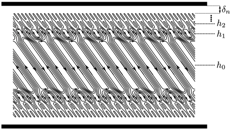
5.1 Parameters for the branching construction

The branching flows consist of several horizontal layers, with the period of the flow doubling from one layer to the next. Within each layer, the velocity field predominantly flows at an angle of $3\pi/4$. See Figure 3 for a sketch. We denote the thickness of the $i$th boundary layer by $\delta_{i}$ for $i\in\{0,\dots n\}$. The relationship between the thicknesses of different boundary layers is governed by

$\displaystyle\delta_{i}=2^{-2}\delta_{i-1},\quad\implies\quad\delta_{i}=2^{-2i}\delta_{0}\quad\text{for all}\quad i\in\{1,\dots n\}.$ (5.1)

Here, $\delta_{0}$ is the thickness of the first layer. The reason for the $2^{-2i}$ decrease in the boundary layer thicknesses will become apparent in later analysis. For the layers lying above and including the midplane ($x_{2}=0$), the $x_{2}$ coordinates of the start of the layers are given by

$\displaystyle h_{0}=0,\qquad h_{i}=\sum_{j=0}^{i-1}\delta_{j}\quad\text{for }i\in\{1,\dots,n+1\}.$ (5.2)

Our branching flow construction is mirror symmetric about the midplane. Therefore, the $x_{2}$ coordinates of the starts of the layers below the midplane simply given by $-h_{i}$. We ensure that the sum of the thicknesses of all these layers (above the midplane) adds up to half the channel width, namely $1/2$, which then leads to

$\displaystyle\sum_{i=0}^{n}\delta_{i}=\frac{1}{2},\quad\implies\quad\delta_{0}\frac{1-2^{-2(n+1)}}{1-2^{-2}}=\frac{1}{2}\quad\implies\quad\frac{1-2^{-2}}{2}\leq\delta_{0}<\frac{1}{2}.$ (5.3)

Consequently, $\delta_{0}$ is $O(1)$, chosen such that (5.3) is satisfied. Next, we denote the typical horizontal wavenumber of the branching flow at the beginning of the $i$th layer by $k_{i}$ for $i\in\{0,\dots n\}$. These wavenumbers obey the following relation

$\displaystyle k_{i}=2k_{i-1},\quad\implies\quad k_{i}=2^{i}k_{0},$ (5.4)

where $k_{0}\in\frac{2\pi}{L}\mathbb{N}$ is the wavenumber at $x_{2}=0$ and will be chosen as part of the proof. In our proof, we will ensure that $\delta_{i}>k_{i}^{-1}$ for $i\in\{0,\dots n\}$, which only requires

$\displaystyle\delta_{n}>k_{n}^{-1}.$ (5.5)

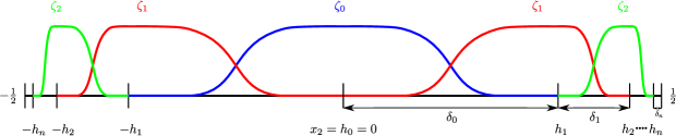
We now define a family of smooth cutoff functions $\zeta_{i}:[-1/2,1/2]\to[0,1]$ for $i\in\{0,\dots n\}$, which satisfy the following properties:

  1. (i)

    $\operatorname{supp}\zeta_{0}\subseteq[-h_{1},h_{1}]$ and $\operatorname{supp}\zeta_{i}\subseteq[-h_{i+1},-h_{i-1}]\cup[h_{i-1},h_{i+1}]$ for $1\leq i\leq n$,

  2. (ii)

    $|\nabla^{j}\zeta_{i}|\leq C_{j}\delta_{i}^{-j},$

  3. (iii)

    $\sum_{i=0}^{n}\zeta_{i}^{2}\leq 1\qquad\text{with}\quad\sum_{i=0}^{n}\zeta_{i}^{2}=1\quad\text{when}\quad x_{2}\in\left[-\frac{1}{2}+\delta_{n},\frac{1}{2}-\delta_{n}\right].$

One can indeed find such a family of cutoff function. For example, following Doering and Tobasco, (2019), we can choose

$\displaystyle\zeta_{i}(x_{2})=f_{i}(x_{2})+f_{i-1}(\delta_{i}+2h_{i}-x_{2})\quad\text{for}\quad x_{2}\in[0,1/2]\quad\text{and}\quad\zeta_{i}(x_{2})=\zeta_{i}(-x_{2})\quad\text{for}\quad x_{2}\in[-1/2,0],$ (5.6)

where

$\displaystyle f(x_{2})=\sqrt{\frac{1}{2}-\frac{1}{2}\tanh\left(\frac{x_{2}-\frac{1}{2}}{x_{2}^{2}(1-x_{2})^{2}}\right)},$ (5.7)
$\displaystyle f_{i}(x_{2})=f\left(\frac{x_{2}-h_{i}}{\delta_{i}}\right)\text{ for }i\in\{0,\dots n-1\},\quad f_{n}(x_{2})=f\left(\frac{x_{2}-h_{n}}{(\delta_{n}/2)}\right)\text{ and }f_{-1}\equiv 0.$

The item (iii) holds because the function $f$ has the properties: $f^{2}\leq 1$ and $f^{2}(x_{2})+f^{2}(1-x_{2})=1$.

Refer to caption
Figure 4: shows cutoff functions $\zeta_{i}$.

5.2 Choice of the velocity field $\boldsymbol{U}$ and $\widetilde{\boldsymbol{v}}$

We write the velocity field $\boldsymbol{U}$ as a sum of two divergence-free velocity fields $\boldsymbol{U}=\boldsymbol{U}^{m}+\boldsymbol{U}^{b}$. We define the mean velocity $\boldsymbol{U}^{m}$ as in (4.7) with $\delta$ replaced with $\delta_{n}$. We define $\boldsymbol{U}^{b}$ and $\widetilde{\boldsymbol{v}}$ based on streamfunctions as

$\displaystyle\Psi(\boldsymbol{x})\coloneqq-\sum_{i=0}^{n}\mathcal{A}\;\zeta_{i}(x_{2})\;\frac{\sin(k_{i}(x_{1}+x_{2}))}{k_{i}},\qquad\boldsymbol{U}_{b}\coloneqq\nabla^{\perp}\Psi,$ (5.8)
$\displaystyle\widetilde{\psi}(\boldsymbol{x})\coloneqq-\sum_{i=0}^{n}\mathfrak{a}\;\zeta_{i}(x_{2})\;\frac{\sin(k_{i}(x_{1}+x_{2}))}{k_{i}},\qquad\widetilde{\boldsymbol{v}}\coloneqq\nabla^{\perp}\widetilde{\psi}.$ (5.9)

Therefore, the choice of $\boldsymbol{U}_{b}$ and $\widetilde{\boldsymbol{v}}$ only differ in the prefactors. From our choices it is clear that

$\displaystyle\operatorname{supp}_{z}\boldsymbol{U}^{m}\subseteq\left[-\frac{1}{2},-\frac{1}{2}+\frac{\delta_{n}}{5}\right)\cup\left(\frac{1}{2}-\frac{\delta_{n}}{5},\frac{1}{2}\right]\text{ and }\operatorname{supp}_{z}\boldsymbol{U}^{b},\operatorname{supp}_{z}\widetilde{\boldsymbol{v}}\subseteq\left[-\frac{1}{2}+\frac{\delta_{n}}{2},\frac{1}{2}-\frac{\delta_{n}}{2}\right].$ (5.10)

The property about the support of $\boldsymbol{U}^{b}$ and $\widetilde{\boldsymbol{v}}$ is true because the function $f_{n}$ in (5.7) is defined based on the boundary layer thickness $\delta_{n}/2$. Next, we have the following estimate on $\nabla\boldsymbol{U}^{b}$:

$\displaystyle\nu\langle|\nabla\boldsymbol{U}^{b}|^{2}\rangle\lesssim\nu\mathcal{A}^{2}\sum_{i=0}^{n}\left(k_{i}^{2}\delta_{i}+\frac{1}{k_{i}^{2}\delta_{i}^{3}}\right)\lesssim\nu\mathcal{A}^{2}k_{0}^{2}\delta_{0}n,$ (5.11)

where we used (5.1), (5.4) and (5.5) to obtain the last relation. Now, we can find an estimate on $\nabla\boldsymbol{U}^{m}$ as in (4.10) with $\delta$ replaced with $\delta_{n}$. Finally, noting the information about the support in (5.10), we get

$\displaystyle C_{l}\frac{\nu}{\delta_{n}}\leq\nu\langle|\nabla\boldsymbol{U}|^{2}\rangle\leq C\left(\frac{\nu}{\delta_{n}}+\nu\mathcal{A}^{2}k_{0}^{2}\delta_{0}n\right),$ (5.12)

for constants $C_{l}$ and $C$ independent of viscosity.

5.3 Estimate on terms $I$, $II$ and $III$

In the calculation of $I=-2\langle U_{2}\widetilde{v}_{1}\rangle$, only the interactions of the same modes in $U_{2}$ and $\widetilde{v}_{1}$ survive, which leads to

$\displaystyle I=-2\left\langle\mathfrak{a}\mathcal{A}\sum_{i=0}^{n}\zeta_{i}^{2}\cos^{2}(k_{i}(x_{1}+x_{2}))\right\rangle\geq\frac{\mathfrak{a}\mathcal{A}}{2}.$ (5.13)

Here, we used that $\delta_{n}\leq 1/4$ and item (iii) about properties of $\zeta_{i}$ in subsection 5.1. The calculation of term $II$ is similar to (5.11), which yields

$\displaystyle II=-\nu\langle|\nabla\widetilde{\boldsymbol{v}}|^{2}\rangle\geq-C_{2}\mathfrak{a}^{2}k_{0}^{2}\delta_{0}n.$ (5.14)

Estimate on term $III$ requires a few steps. We first write down

$\displaystyle\boldsymbol{U}\cdot\nabla\widetilde{\boldsymbol{v}}=\overline{\boldsymbol{W}}+\widetilde{\boldsymbol{W}},$ (5.15)

where we define the components of $\overline{\boldsymbol{W}}$ and $\widetilde{\boldsymbol{W}}$ as follows

$\displaystyle(\boldsymbol{U}\cdot\nabla\widetilde{\boldsymbol{v}})_{1}$ $\displaystyle=\overline{W}_{1}+\widetilde{W}_{1}$
โ‰”โˆ’๐”žโ€‹๐’œโ€‹(ฮถiโ€‹ฮถiโ€ฒ+ฮถi+1โ€‹ฮถi+1โ€ฒ)+(โˆ‘j=14ฮฑjcโ€‹cosโก(jโ€‹kiโ€‹(x1+x2))+โˆ‘j=14ฮฑjsโ€‹sinโก(jโ€‹kiโ€‹(x1+x2))),โ‰”absent๐”ž๐’œsubscript๐œ๐‘–superscriptsubscript๐œ๐‘–โ€ฒsubscript๐œ๐‘–1superscriptsubscript๐œ๐‘–1โ€ฒsuperscriptsubscript๐‘—14subscriptsuperscript๐›ผ๐‘๐‘—๐‘—subscript๐‘˜๐‘–subscript๐‘ฅ1subscript๐‘ฅ2superscriptsubscript๐‘—14subscriptsuperscript๐›ผ๐‘ ๐‘—๐‘—subscript๐‘˜๐‘–subscript๐‘ฅ1subscript๐‘ฅ2\displaystyle\coloneqq-\mathfrak{a}\mathcal{A}\left(\zeta_{i}\zeta_{i}^{\prime}+\zeta_{i+1}\zeta_{i+1}^{\prime}\right)+\left(\sum_{j=1}^{4}\alpha^{c}_{j}\cos(jk_{i}(x_{1}+x_{2}))+\sum_{j=1}^{4}\alpha^{s}_{j}\sin(jk_{i}(x_{1}+x_{2}))\right), (5.16)
$\displaystyle(\boldsymbol{U}\cdot\nabla\widetilde{\boldsymbol{v}})_{2}$ $\displaystyle=\overline{W}_{2}+\widetilde{W}_{2}\coloneqq\mathfrak{a}\mathcal{A}\left(\zeta_{i}\zeta_{i}^{\prime}+\zeta_{i+1}\zeta_{i+1}^{\prime}\right)-\sum_{j=1}^{4}\alpha^{c}_{j}\cos(jk_{i}(x_{1}+x_{2})).$ (5.17)

We note the coefficients $\alpha^{c}_{j}$ and ฮฑjssubscriptsuperscript๐›ผ๐‘ ๐‘—\alpha^{s}_{j} in (5.16) and (5.17) are smooth function of $x_{2}$ and are given by

$\displaystyle\alpha^{c}_{1}=-\frac{3}{4}\mathfrak{a}\mathcal{A}(2\zeta_{i+1}\zeta_{i}^{\prime}+\zeta_{i}\zeta_{i+1}^{\prime}),\qquad\alpha^{c}_{2}=0,\qquad\alpha^{c}_{3}=\frac{1}{4}\mathfrak{a}\mathcal{A}(2\zeta_{i+1}\zeta_{i}^{\prime}-\zeta_{i}\zeta_{i+1}^{\prime}),\qquad\alpha^{c}_{4}=0,$ (5.18)
ฮฑ1s=โˆ’14โ€‹kiโ€‹๐”žโ€‹๐’œโ€‹(ฮถiโ€ฒโ€‹ฮถi+1โ€ฒโˆ’2โ€‹ฮถi+1โ€‹ฮถiโ€ฒโ€ฒ+ฮถiโ€‹ฮถi+1โ€ฒโ€ฒ),ฮฑ2s=12โ€‹kiโ€‹๐”žโ€‹๐’œโ€‹((ฮถiโ€ฒ)2โˆ’ฮถiโ€‹ฮถiโ€ฒโ€ฒ),formulae-sequencesubscriptsuperscript๐›ผ๐‘ 114subscript๐‘˜๐‘–๐”ž๐’œsuperscriptsubscript๐œ๐‘–โ€ฒsuperscriptsubscript๐œ๐‘–1โ€ฒ2subscript๐œ๐‘–1superscriptsubscript๐œ๐‘–โ€ฒโ€ฒsubscript๐œ๐‘–superscriptsubscript๐œ๐‘–1โ€ฒโ€ฒsubscriptsuperscript๐›ผ๐‘ 212subscript๐‘˜๐‘–๐”ž๐’œsuperscriptsuperscriptsubscript๐œ๐‘–โ€ฒ2subscript๐œ๐‘–superscriptsubscript๐œ๐‘–โ€ฒโ€ฒ\displaystyle\alpha^{s}_{1}=-\frac{1}{4k_{i}}\mathfrak{a}\mathcal{A}\left(\zeta_{i}^{\prime}\zeta_{i+1}^{\prime}-2\zeta_{i+1}\zeta_{i}^{\prime\prime}+\zeta_{i}\zeta_{i+1}^{\prime\prime}\right),\qquad\alpha^{s}_{2}=\frac{1}{2k_{i}}\mathfrak{a}\mathcal{A}\left((\zeta_{i}^{\prime})^{2}-\zeta_{i}\zeta_{i}^{\prime\prime}\right), (5.19)
ฮฑ3s=14โ€‹kiโ€‹๐”žโ€‹๐’œโ€‹(3โ€‹ฮถiโ€ฒโ€‹ฮถi+1โ€ฒโˆ’ฮถi+1โ€‹ฮถiโ€ฒโ€ฒโˆ’ฮถiโ€‹ฮถi+1โ€ฒโ€ฒ),ฮฑ4s=14โ€‹kiโ€‹๐”žโ€‹๐’œโ€‹((ฮถi+1โ€ฒ)2โˆ’ฮถi+1โ€‹ฮถi+1โ€ฒโ€ฒ).formulae-sequencesubscriptsuperscript๐›ผ๐‘ 314subscript๐‘˜๐‘–๐”ž๐’œ3superscriptsubscript๐œ๐‘–โ€ฒsuperscriptsubscript๐œ๐‘–1โ€ฒsubscript๐œ๐‘–1superscriptsubscript๐œ๐‘–โ€ฒโ€ฒsubscript๐œ๐‘–superscriptsubscript๐œ๐‘–1โ€ฒโ€ฒsubscriptsuperscript๐›ผ๐‘ 414subscript๐‘˜๐‘–๐”ž๐’œsuperscriptsuperscriptsubscript๐œ๐‘–1โ€ฒ2subscript๐œ๐‘–1superscriptsubscript๐œ๐‘–1โ€ฒโ€ฒ\displaystyle\alpha^{s}_{3}=\frac{1}{4k_{i}}\mathfrak{a}\mathcal{A}\left(3\zeta_{i}^{\prime}\zeta_{i+1}^{\prime}-\zeta_{i+1}\zeta_{i}^{\prime\prime}-\zeta_{i}\zeta_{i+1}^{\prime\prime}\right),\qquad\alpha^{s}_{4}=\frac{1}{4k_{i}}\mathfrak{a}\mathcal{A}\left((\zeta_{i+1}^{\prime})^{2}-\zeta_{i+1}\zeta_{i+1}^{\prime\prime}\right). (5.20)

Enforcing the condition (5.5), we note one important estimate on these coefficients:

$\displaystyle\|\alpha^{c}_{j}\|_{L^{\infty}},\|\alpha^{s}_{j}\|_{L^{\infty}},\leq c\mathfrak{a}\mathcal{A}\delta_{i}^{-1},$ (5.21)

for some constant $c$ independent of $j$ and $\nu$. Now, an estimate on term $III$ can be written as

$\displaystyle|III|=\nu^{-1}\langle|\nabla\Delta^{-1}\mathbb{P}\boldsymbol{U}\cdot\nabla\widetilde{\boldsymbol{v}}|^{2}\rangle\leq 2\nu^{-1}\langle|\nabla\Delta^{-1}\mathbb{P}\overline{\boldsymbol{W}}|^{2}\rangle+2\nu^{-1}\langle|\nabla\Delta^{-1}\mathbb{P}\widetilde{\boldsymbol{W}}|^{2}\rangle\eqcolon E_{1}+E_{2}.$ (5.22)

We first focus on estimating $E_{1}$. From (5.16) and (5.17), we notice that

$\displaystyle\overline{\boldsymbol{W}}=\left(-\frac{\mathfrak{a}\mathcal{A}}{2},\frac{\mathfrak{a}\mathcal{A}}{2}\right)^{T}\sum_{i=0}^{n}(\zeta_{i}^{2})^{\prime}.$ (5.23)

Next, we observe that for a smooth function $f(x_{1},x_{2})\coloneq f(x_{2})$, which satisfies $f(-1/2)=f(1/2)=0$, we have $\mathbb{P}(0,\partial_{x_{2}}f)=0$. Therefore, we can write

$$\nu^{-1}\langle|\nabla\Delta^{-1}\mathbb{P}\overline{\boldsymbol{W}}|^{2}\rangle=\nu^{-1}\langle|\nabla\Delta^{-1}\overline{W}_{1}|^{2}\rangle.$$

This is because $\mathbb{P}(\overline{W}_{1},0)=(\overline{W}_{1},0)$ as $\overline{W}_{1}$ is only a function of $x_{2}$. To estimate $\nu^{-1}\langle|\nabla\Delta^{-1}\overline{W}_{1}|^{2}\rangle$, we note the following lemma.

Lemma 5.1.

Let $f(x_{1},x_{2})\coloneqq f(x_{2})$ be a nonnegative smooth function such that $f(x_{2})\leq 1$ and $f(x_{2})=1$ when $x_{2}\in[-1/2+\delta,1/2-\delta]$ for some $\delta\leq 1/4$. Then

$\displaystyle\mathchoice{{\vbox{\hbox{$\textstyle-$ }}\kern-7.83337pt}}{{\vbox{\hbox{$\scriptstyle-$ }}\kern-5.90005pt}}{{\vbox{\hbox{$\scriptscriptstyle-$ }}\kern-4.75003pt}}{{\vbox{\hbox{$\scriptscriptstyle-$ }}\kern-4.25003pt}}\!\int_{\Omega}|\nabla\Delta^{-1}\partial_{x_{2}}f|^{2}\,{\rm d}\boldsymbol{x}\leq 6\delta.$ (5.24)
Proof.

We note that

$\displaystyle\Delta^{-1}\partial_{x_{2}}f=\int_{-\frac{1}{2}}^{x_{2}}f(x_{2}^{\prime})\,{\rm d}x_{2}^{\prime}-\left(x_{2}+\frac{1}{2}\right)\int_{-\frac{1}{2}}^{\frac{1}{2}}f(x_{2}^{\prime})\,{\rm d}x_{2}^{\prime},$ (5.25)

which implies

$\displaystyle\nabla\Delta^{-1}\partial_{x_{2}}f=f(x_{2})-\int_{-\frac{1}{2}}^{\frac{1}{2}}f(x_{2}^{\prime})\,{\rm d}x_{2}^{\prime}.$ (5.26)

Therefore, we have

$\displaystyle|\nabla\Delta^{-1}\partial_{x_{2}}f|\leq|1-f(x_{2})|+\left|1-\int_{-\frac{1}{2}}^{\frac{1}{2}}f(x_{2}^{\prime})\,{\rm d}x_{2}^{\prime}\right|\leq|1-f(x_{2})|+2\delta.$ (5.27)

Therefore, we get the following bound

$\displaystyle|\nabla\Delta^{-1}\partial_{x_{2}}f|\leq\begin{cases}1+2\delta\quad&\text{when}\quad x_{2}\left(-\frac{1}{2},-\frac{1}{2}+\delta\right)\cup\left(\frac{1}{2}+\delta,\frac{1}{2}\right),\\ 2\delta\quad&\text{when}\quad x_{2}\in\left[-\frac{1}{2}+\delta,\frac{1}{2}-\delta\right].\end{cases}$ (5.28)

Finally, a volume integration gives the required bound (5.24). โˆŽ

Since, we have $\overline{W}_{1}=-\partial_{x_{2}}(\mathfrak{a}\mathcal{A}\sum_{i=0}^{n}\zeta_{i}^{2}/2)$, using Lemma 5.1, we obtain the following bound:

$\displaystyle E_{1}\lesssim\nu^{-1}\mathfrak{a}^{2}\mathcal{A}^{2}\delta_{n}.$ (5.29)

Next, we estimate $E_{2}$ in (5.22) as follows:

$\displaystyle 2\nu^{-1}\langle|\nabla\Delta^{-1}\mathbb{P}\widetilde{\boldsymbol{W}}|^{2}\rangle$ $\displaystyle=2\nu^{-1}\left\langle\left|\nabla\Delta^{-1}\mathbb{P}\partial_{x_{1}}\scaleobj{.8}{\int_{0}^{x_{1}}}\widetilde{\boldsymbol{W}}(x_{1}^{\prime},x_{2})\,{\rm d}x_{1}^{\prime}\right|^{2}$
$\displaystyle\lesssim\nu^{-1}\left\langle\left|\scaleobj{.8}{\int_{0}^{x_{1}}}\widetilde{\boldsymbol{W}}(x_{1}^{\prime},x_{2})\,{\rm d}x_{1}^{\prime}\right|^{2}\right\rangle$
$\displaystyle\lesssim\nu^{-1}\mathfrak{a}^{2}\mathcal{A}^{2}\sum_{i=0}^{n}\frac{1}{k_{i}^{2}\delta_{i}}$
$\displaystyle\lesssim C\nu^{-1}\mathfrak{a}^{2}\mathcal{A}^{2}\frac{n}{k_{0}^{2}\delta_{0}}.$ (5.30)

The function $\scaleobj{.8}{\int_{0}^{x_{1}}}\widetilde{\boldsymbol{W}}(x_{1}^{\prime},x_{2})\,{\rm d}x_{1}^{\prime}$ is periodic in $x_{1}$ and is therefore well-defined on $\Omega$. To obtain the second line in (5.30), we used the fact that $\nabla\Delta^{-1}\mathbb{P}\partial_{x_{1}}$ is a Calderรณnโ€“Zygmund operator of zeroth-order. To obtain the last line, we note that

$\displaystyle\left|\scaleobj{.8}{\int_{0}^{x_{1}}}\widetilde{\boldsymbol{W}}(x_{1}^{\prime},x_{2})\,{\rm d}x_{1}^{\prime}\right|\lesssim\frac{\mathfrak{a}\mathcal{A}}{k_{i}\delta_{i}},\quad\text{when}\quad x_{2}\in[-h_{i+1},h_{i}]\cup[h_{i},h_{i+1}].$ (5.31)

Combining (5.29) and (5.30), we get an estimate on term $III$:

$\displaystyle|III|$ $\displaystyle\leq C_{3}\nu^{-1}\mathfrak{a}^{2}\mathcal{A}^{2}\left(\frac{\delta_{0}}{2^{2n}}+\frac{n}{k_{0}^{2}\delta_{0}}\right)$ (5.32)

5.4 Proof of Theorem 1.5

We make the following choice of the parameters:

๐’œ=1log2โกฮฝโˆ’1,๐”ž=๐” log2โกฮฝโˆ’1,formulae-sequence๐’œ1subscript2superscript๐œˆ1๐”ž๐” subscript2superscript๐œˆ1\displaystyle\qquad\qquad\qquad\mathcal{A}=\frac{1}{\log_{2}\nu^{-1}},\qquad\qquad\mathfrak{a}=\frac{\mathfrak{c}}{\log_{2}\nu^{-1}}, (5.33)
$\displaystyle\frac{1}{\nu^{\frac{1}{2}}\left(\log_{2}\nu^{-1}\right)^{\frac{1}{2}}}<k_{0}\leq\frac{1}{\nu^{\frac{1}{2}}\left(\log_{2}\nu^{-1}\right)^{\frac{1}{2}}}+\frac{2\pi}{L},\qquad n=\left\lfloor\frac{1}{2}\log_{2}\left(\frac{1}{\nu\log_{2}^{2}\nu^{-1}}\right)\right\rfloor.$ (5.34)

With these choices, from (5.12), we see that $\nu\langle|\nabla\boldsymbol{U}|^{2}\rangle\sim(\log_{2}\nu^{-1})^{-2}.$ Next, we see that the estimates (5.13), (5.14) and (5.32) for terms $I$, $II$ and $III$, respectively, also scale as $(\log_{2}\nu^{-1})^{-2}.$ Therefore, by choosing ๐” ๐” \mathfrak{c} to be small enough, we get that $\nu\langle|\nabla\boldsymbol{u}|^{2}\rangle\gtrsim(\log_{2}\nu^{-1})^{-2}.$ Finally, to satisfy the condition (5.5), along with the constraint $\delta_{n}\leq 1/4$, we require $\nu<1/500.$

6 Conclusion and future outlook

In this paper, we explored the phenomenon of anomalous and enhanced dissipation in a passive divergence-free vector field in a Couette flow setting. One of the main result of the paper is an upper bound on the rate of energy dissipation $\varepsilon_{\boldsymbol{u}}$ in the passive vector field $\boldsymbol{u}$ in terms of the energy dissipation $\varepsilon_{\boldsymbol{U}}$in the convecting vector field $\boldsymbol{U}$ (see Theorem 1.4). Complementary to this upper bound, in Theorem 1.5, we provided a construction of a family of convecting vector fields $\{\boldsymbol{U}_{\nu}\}_{\nu>0}$ dissipating energy as $(\log\nu^{-1})^{2}$ for which the energy dissipation in the passive vector $\boldsymbol{u}$ goes at least as $(\log\nu^{-1})^{2}$. The proof of this result is based on a variational principle for the rate of energy dissipation given in Section 3. Our results in Theorem 1.4 and Theorem 1.5 can be restated in terms of the momentum transport or the transverse current of stream-wise ($x_{1}$) component of velocity $\boldsymbol{u}$:

$\displaystyle J^{\boldsymbol{u}}=\nu\overline{\partial_{2}u_{1}}-\overline{U_{2}u_{1}},$ (6.1)

as $J^{\boldsymbol{u}}$ relates to energy dissipation through formula (2.5).

In the context of the incompressible vector diffusion equation, a key question of interest is Question 1.2 in the Couette flow setting. Most studies on anomalous dissipation in passive scalars rely on the Lagrangian viewpoint, which cannot be directly applied to the passive vector equation considered in this paper. Consequently, addressing this question requires novel approaches that go beyond traditional Lagrangian methods. The variational approach presented in this paper could be one such potential method of tackling this question. We used two-dimensional branching flows within the variational principle, which allows us to answer this question with a logarithmic scaling discrepancy. It is known from the studies of optimal scalar transport problems, that two-dimensional branching flows lead to a logarithmic scaling miss (Doering and Tobasco,, 2019). In (Kumar,, 2022; Kumar, 2023a, ), it was shown that such logarithmic correction can be eliminated (thus achieving the clean scaling of optimal scalar transport) through the use of three-dimensional branching flows. Consequently, it is plausible that, in the context of passive vector fields as well, a construction based on three-dimensional branching flows could fully resolve Question 1.2. Another promising approach that can be fruitful is due to Armstrong and Vicol, (2023) on anomalous dissipation in a passive scalar, which is based on homogenization techniques. It would be interesting to see whether their approach can be adapted to resolve this question.

We note that Question 1.2 may likely be answered by considering a freely decaying flow, i.e., a flow within a periodic domain or a smooth bounded domain with homogeneous Dirichlet boundary conditions, in the absence of forcing, starting from an initial condition $\boldsymbol{u}_{0}$ independent of viscosity. In this scenario, the long-time average should be replaced with a finite-time average. We can consider this problem in three dimensions and choose the velocity fields of the form $\boldsymbol{U}=(U_{1}(x_{1},x_{2}),U_{2}(x_{1},x_{2}),0)$ and $\boldsymbol{u}=(0,0,u_{3}(x_{1},x_{2}))$. The governing equation for $u_{3}$ then becomes the advection-diffusion equation. Finally, to answer Question 1.2 one might consider choosing $\boldsymbol{U}$ as an alternating shear flow or a checkered board flow, as employed by (Drivas etย al.,, 2022; Colombo etย al.,, 2023; Elgindi and Liss,, 2023) in studies of anomalous dissipation in a passive scalar. However, we do not pursue this solution in this paper because the velocity fields $\boldsymbol{U}$ and $\boldsymbol{u}$ differ significantly, which we think is an artifact of the finite-time average. Consequently, such a solution is unlikely to exist in the settings discussed in the Introduction, where there is a continuous supply of energy at the larger scales and a long-time average is used in the definition of energy dissipation, which renders the transient nature of the problem irrelevant. But more importantly, our future interest lies in the potential to close the gap between $\boldsymbol{U}$ and $\boldsymbol{u}$ using computational tools, which is the primary motivation for this study. Because $\boldsymbol{U}$ and $\boldsymbol{u}$ described above are so distinct that it seems unlikely they could be unified to obtain a solution to the Navierโ€“Stokes equation. For example, such a solution does not appear to work when the number of input/output passes are increased to $n=2$ (see Question 6.3 below).

We conclude the paper by noting a few problems based on the input/output perspective taken in this paper, where we believe it is possible to make progress using both analysis and computational tools and can provide valuable insights into the solutions of Navierโ€“Stokes equation. The first problem is related to optimal mixing of a passive scalar in the limit of zero diffusion, which has been a focus of recent studies. For cases where the underlying vector field is Sobolev, $\boldsymbol{U}\in L^{\infty}_{t}W_{\boldsymbol{x}}^{1,p}$, this problem has been examined using both computational approaches (Lin etย al.,, 2011; Iyer etย al.,, 2014) and rigorous upper (Crippa and Deย Lellis,, 2008; Seis,, 2013; Iyer etย al.,, 2014) and lower bounds (Yao and Zlatoลก,, 2017; Alberti etย al.,, 2019; Elgindi and Zlatoลก,, 2019), demonstrating that the optimal mixing rate is exponential in time. However, one crucial drawback of these studies is that the velocity field lacks a governing equation. In particular, the velocity field does not arise as a solution of the Navierโ€“Stokes equation in one of the three settings discussed in the Introduction. The point of view taken in this paper can remedy this gap to certain extent. In particular, we ask whether the exponential mixing still holds if the vector field $\boldsymbol{u}$ is a solution of (1.1a-b) and convects a scalar $\theta$:

Question 6.1 (Mixing of a scalar).

Consider the advection of a scalar $\theta$, $\partial_{t}\theta+\boldsymbol{u}\cdot\nabla\theta=0$, by a divergence-free velocity field $\boldsymbol{u}$ which itself is obtained from solving $\partial_{t}\boldsymbol{u}+\boldsymbol{U}\cdot\nabla\boldsymbol{u}=-\nabla p+\nu\Delta\boldsymbol{u}$. The velocity field $\boldsymbol{U}$ is smooth divergence free and satisfies the bound $\left\lVert\boldsymbol{U}(t,\cdot)\right\rVert_{W^{1,p}}\leq B$. Is it then true that for s<0๐‘ 0s<0, โˆฅฮธโ€‹(t,โ‹…)โˆฅHsโ‰ฅexpโก(โˆ’cโ€‹Bโ€‹t)subscriptdelimited-โˆฅโˆฅ๐œƒ๐‘กโ‹…superscript๐ป๐‘ ๐‘๐ต๐‘ก\left\lVert\theta(t,\cdot)\right\rVert_{H^{s}}\geq\exp(-cBt) for some constant $c$ independent of $B$.

A complementary question would be if exponential mixing is a lower bound then is it sharp, i.e., can one produce examples of $\boldsymbol{U}$ for which the exponential mixing holds? A similar question can be asked regarding the mixing behavior of a passive vector field.

Question 6.2 (Mixing of a vector).

Consider the advection of a vector of a divergence-free velocity field $\boldsymbol{u}$ which itself is obtained from solving $\partial_{t}\boldsymbol{u}+\boldsymbol{U}\cdot\nabla\boldsymbol{u}=-\nabla p$. The velocity field $\boldsymbol{U}$ is smooth divergence free and satisfies the bound $\left\lVert\boldsymbol{U}(t,\cdot)\right\rVert_{W^{1,p}}\leq B$. Is it then true that for s<0๐‘ 0s<0, โˆฅ๐ฎโ€‹(t,โ‹…)โˆฅHsโ‰ฅexpโก(โˆ’cโ€‹Bโ€‹t)subscriptdelimited-โˆฅโˆฅ๐ฎ๐‘กโ‹…superscript๐ป๐‘ ๐‘๐ต๐‘ก\left\lVert\boldsymbol{u}(t,\cdot)\right\rVert_{H^{s}}\geq\exp(-cBt) for some constant $c$ independent of $B$.

The equation (1.1) discussed in this paper represents a single level of input/output pass. However, one could more broadly consider the mixing questions mentioned above or the problem of anomalous dissipation within a framework involving multiple levels of input/output pass. For instance, one might ask

Question 6.3 (Multiple input/output passes).

Consider a set of partial differential equations

$\displaystyle\partial_{t}\boldsymbol{u}_{i}+\boldsymbol{u}_{i-1}\cdot\nabla\boldsymbol{u}_{i}=-\nabla p_{i}+\nu\Delta\boldsymbol{u}_{i}\qquad i\in\{1,\dots n\},$ (6.2)

where the velocity field $\boldsymbol{u}_{i}$ for all $i\in\{0,\dots n\}$ are divergence-free. Is it possible to produce an example of smooth velocity fields $\boldsymbol{u}_{0}$ which exhibit anomalous dissipation such that $\nu\langle|\nabla\boldsymbol{u}_{n}|^{2}\rangle\geq c_{n}>0,$ where $c_{n}$ is a constant independent of the viscosity. A more challenging question is whether $c_{n}$ can also be made independent of $n$.

The fixed point iteration (6.2) (without the time derivative) is used to find numerical solution of the steady Navierโ€“Stokes equation (Kay etย al.,, 2002) and goes by the name of Arrowโ€“Hurwicz algorithm (Temam,, 2024).

Next, we consider the Naiverโ€“Stokes equation under the Boussinesq approximation coupled with the advection-diffusion equation. However, we replace the term $\boldsymbol{u}\cdot\nabla\boldsymbol{u}$ by $\boldsymbol{U}\cdot\nabla\boldsymbol{u}$. Consequently, the momentum part of the equation becomes linear but the interaction of $\boldsymbol{u}$ with $T$ in the convection-diffusion equation leads to nonlinearity. One can consider these equations, for example, in the standard Raylieghโ€“Bรฉnard setup. The Rayleighโ€“Bรฉnard convection (RBC) is the flow driven by buoyancy in a differentially heated layer of fluid. In particular, the velocity fields $\boldsymbol{U}$ and $\boldsymbol{u}$ satisfy homogeneous Dirichlet boundary condition and the temperature $T=1$ at $x_{2}=-1/2$ and $T=0$ at $x_{2}=0$. The two nondimensional parameters governing the equations are the Rayleigh number (based on $1$ unit gap width and $1$ unit temperature difference) $Ra=\nu^{-1}\kappa^{-1}g\alpha$ and the Prandtl number $Pr=\kappa^{-1}\nu$, where $\nu$, $\kappa$, $\alpha$ and $g$ are the viscosity, thermal diffusivity, coefficient of thermal expansion and the gravitational acceleration, respectively. The Nusselt number, which quantifies nondimensional heat transfer, is given by $Nu=\langle|\nabla T|^{2}\rangle=1+\langle u_{2}T\rangle=1+Ra^{-1}\langle|\nabla\boldsymbol{u}|^{2}\rangle$. One of the competing theories of heat transfer suggests that for Prandtl number order one, the dimensional rate of heat transfer becomes independent of the molecular diffusion (upto possibly a logarithmic correction) in the limit of large Rayleigh number, which in terms of Nusselt number is $Nu\sim Ra^{1/2}$ (Kraichnan,, 1962; Grossmann and Lohse,, 2000). This rate of heat transfer leads to anomalous dissipation in the velocity field $\boldsymbol{u}$. Given this prediction, we pose the following question, which is presumably easier to answer than the full nonlinear system (the Naiverโ€“Stokes equation under the Boussinesq approximation) but more challenging than a purely linear system.

Question 6.4 (A nonlinear problem).

Consider the following set of equations

$\displaystyle\partial_{t}\boldsymbol{u}+\boldsymbol{U}\cdot\nabla\boldsymbol{u}=-\nabla p+Pr\Delta\boldsymbol{u}+PrRaT\boldsymbol{e}_{2},$ (6.3)
$\displaystyle\partial_{t}T+\boldsymbol{u}\cdot\nabla T=\Delta T,$ (6.4)

where both of the velocity fields $\boldsymbol{u}$ and $\boldsymbol{U}$ are divergence-free. Is it possible to produce example of smooth vector fields $\boldsymbol{U}$ for which $Ra^{-1}\langle|\nabla\boldsymbol{U}|^{2}\rangle\sim Ra^{1/2}$ such that there is a solution $(\boldsymbol{u},T)$ satisfying $Ra^{-1}\langle|\nabla\boldsymbol{u}|^{2}\rangle=\langle u_{2}T\rangle\gtrsim Ra^{1/2}$ as $Ra\to\infty$.

References

  • Alberti etย al., (2019) Alberti, G., Crippa, G., and Mazzucato, A.ย L. (2019). Exponential self-similar mixing by incompressible flows. J. Amer. Math. Soc., 32(2):445โ€“490.
  • Armstrong and Vicol, (2023) Armstrong, S. and Vicol, V. (2023). Anomalous diffusion by fractal homogenization. arXiv preprint arXiv:2305.05048.
  • Bruรจ etย al., (2024) Bruรจ, E., Colombo, M., and Kumar, A. (2024). Sharp Nonuniqueness in the Transport Equation with Sobolev Velocity Field. arXiv preprint arXiv:2405.01670.
  • Bruรจ and De Lellis, (2023) Bruรจ, E. and De Lellis, C. (2023). Anomalous Dissipation for the Forced 3D Navier-Stokes Equations. Comm. Math. Phys., 400(3):1507โ€“1533.
  • Colombo etย al., (2023) Colombo, M., Crippa, G., and Sorella, M. (2023). Anomalous dissipation and lack of selection in the Obukhovโ€“Corrsin theory of scalar turbulence. Annals of PDE, 9(2):21.
  • Cotiย Zelati etย al., (2020) Cotiย Zelati, M., Delgadino, M.ย G., and Elgindi, T.ย M. (2020). On the relation between enhanced dissipation timescales and mixing rates. Communications on Pure and Applied Mathematics, 73(6):1205โ€“1244.
  • Crippa and Deย Lellis, (2008) Crippa, G. and Deย Lellis, C. (2008). Estimates and regularity results for the DiPerna-Lions flow.
  • Depauw, (2003) Depauw, N. (2003). Non unicitรฉ des solutions bornรฉes pour un champ de vecteurs BV en dehors dโ€™un hyperplan. Comptes rendus. Mathรฉmatique, 337(4):249โ€“252.
  • Doering and Tobasco, (2019) Doering, C.ย R. and Tobasco, I. (2019). On the optimal design of wall-to-wall heat transport. Comm. Pure Appl. Math., 72(11):2385โ€“2448.
  • Drivas, (2022) Drivas, T.ย D. (2022). Self-regularization in turbulence from the Kolmogorov 4/5-law and alignment. Philosophical Transactions of the Royal Society A, 380(2226):20210033.
  • Drivas etย al., (2022) Drivas, T.ย D., Elgindi, T.ย M., Iyer, G., and Jeong, I.-J. (2022). Anomalous dissipation in passive scalar transport. Archive for Rational Mechanics and Analysis, pages 1โ€“30.
  • Elgindi and Liss, (2023) Elgindi, T.ย M. and Liss, K. (2023). Norm growth, non-uniqueness, and anomalous dissipation in passive scalars. arXiv preprint arXiv:2309.08576.
  • Elgindi and Zlatoลก, (2019) Elgindi, T.ย M. and Zlatoลก, A. (2019). Universal mixers in all dimensions. Adv. Math., 356:106807, 33.
  • Frisch, (1995) Frisch, U. (1995). Turbulence: the legacy of AN Kolmogorov. Cambridge university press.
  • Galdi, (2011) Galdi, G. (2011). An introduction to the mathematical theory of the Navier-Stokes equations: Steady-state problems. Springer Science & Business Media.
  • Grossmann and Lohse, (2000) Grossmann, S. and Lohse, D. (2000). Scaling in thermal convection: a unifying theory. Journal of Fluid Mechanics, 407:27โ€“56.
  • Hassanzadeh etย al., (2014) Hassanzadeh, P., Chini, G.ย P., and Doering, C.ย R. (2014). Wall to wall optimal transport. J. Fluid. Mech., 751:627โ€“662.
  • Hellstrรถm etย al., (2016) Hellstrรถm, L.ย H., Marusic, I., and Smits, A.ย J. (2016). Self-similarity of the large-scale motions in turbulent pipe flow. Journal of Fluid Mechanics, 792:R1.
  • Hwang, (2015) Hwang, Y. (2015). Statistical structure of self-sustaining attached eddies in turbulent channel flow. Journal of Fluid Mechanics, 767:254โ€“289.
  • Iyer etย al., (2014) Iyer, G., Kiselev, A., and Xu, X. (2014). Lower bounds on the mix norm of passive scalars advected by incompressible enstrophy-constrained flows. Nonlinearity, 27(5):973.
  • Iyer and Van, (2022) Iyer, G. and Van, T.-S. (2022). Bounds on the heat transfer rate via passive advection. SIAM J. Math. Anal., 54(2):1927โ€“1965.
  • Kaneda etย al., (2003) Kaneda, Y., Ishihara, T., Yokokawa, M., Itakura, K., and Uno, A. (2003). Energy dissipation rate and energy spectrum in high resolution direct numerical simulations of turbulence in a periodic box. Physics of Fluids, 15(2):L21โ€“L24.
  • Kawahara etย al., (2012) Kawahara, G., Uhlmann, M., and Vanย Veen, L. (2012). The significance of simple invariant solutions in turbulent flows. Annual Review of Fluid Mechanics, 44(1):203โ€“225.
  • Kay etย al., (2002) Kay, D., Loghin, D., and Wathen, A. (2002). A preconditioner for the steady-state Navierโ€“Stokes equations. SIAM Journal on Scientific Computing, 24(1):237โ€“256.
  • Kraichnan, (1962) Kraichnan, R.ย H. (1962). Turbulent thermal convection at arbitrary Prandtl number. The Physics of Fluids, 5(11):1374โ€“1389.
  • Kumar, (2022) Kumar, A. (2022). Three dimensional branching pipe flows for optimal scalar transport between walls. arXiv preprint arXiv:2205.03367.
  • (27) Kumar, A. (2023a). Bulk properties and flow structures in turbulent flows. PhD thesis, University of California, Santa Cruz.
  • (28) Kumar, A. (2023b). Nonuniqueness of trajectories on a set of full measure for sobolev vector fields. arXiv preprint arXiv:2301.05185.
  • Lin etย al., (2011) Lin, Z., Thiffeault, J.-L., and Doering, C.ย R. (2011). Optimal stirring strategies for passive scalar mixing. Journal of Fluid Mechanics, 675:465โ€“476.
  • Lozano-Durรกn etย al., (2012) Lozano-Durรกn, A., Flores, O., and Jimรฉnez, J. (2012). The three-dimensional structure of momentum transfer in turbulent channels. Journal of Fluid Mechanics, 694:100โ€“130.
  • Marusic etย al., (2010) Marusic, I., McKeon, B.ย J., Monkewitz, P.ย A., Nagib, H.ย M., Smits, A.ย J., and Sreenivasan, K.ย R. (2010). Wall-bounded turbulent flows at high reynolds numbers: recent advances and key issues. Physics of fluids, 22(6).
  • Marusic etย al., (2013) Marusic, I., Monty, J.ย P., Hultmark, M., and Smits, A.ย J. (2013). On the logarithmic region in wall turbulence. Journal of Fluid Mechanics, 716:R3.
  • McKeon, (2019) McKeon, B.ย J. (2019). Self-similar hierarchies and attached eddies. Physical Review Fluids, 4(8):082601.
  • Nguyenย van Yen etย al., (2011) Nguyenย van Yen, R., Farge, M., and Schneider, K. (2011). Energy dissipating structures produced by walls in two-dimensional flows at vanishing viscosity. Physical Review Letters, 106(18):184502.
  • Pearson etย al., (2002) Pearson, B.ย R., Krogstad, P.-ร…., and vanย de Water, W. (2002). Measurements of the turbulent energy dissipation rate. Physics of fluids, 14(3):1288โ€“1290.
  • Schlichting and Gersten, (2016) Schlichting, H. and Gersten, K. (2016). Boundary-layer theory. springer.
  • Seis, (2013) Seis, C. (2013). Maximal mixing by incompressible fluid flows. Nonlinearity, 26(12):3279.
  • Seis, (2015) Seis, C. (2015). Scaling bounds on dissipation in turbulent flows. J. Fluid Mech., 777:591โ€“603.
  • Smits etย al., (2011) Smits, A.ย J., McKeon, B.ย J., and Marusic, I. (2011). Highโ€“Reynolds number wall turbulence. Annual Review of Fluid Mechanics, 43(1):353โ€“375.
  • Song etย al., (2023) Song, B., Fantuzzi, G., and Tobasco, I. (2023). Bounds on heat transfer by incompressible flows between balanced sources and sinks. Physica D: Nonlinear Phenomena, 444:133591.
  • Souza etย al., (2020) Souza, A.ย N., Tobasco, I., and Doering, C.ย R. (2020). Wall-to-wall optimal transport in two dimensions. J. Fluid. Mech., 889.
  • Sreenivasan, (1984) Sreenivasan, K.ย R. (1984). On the scaling of the turbulence energy dissipation rate. The Physics of fluids, 27(5):1048โ€“1051.
  • Sreenivasan, (1998) Sreenivasan, K.ย R. (1998). An update on the energy dissipation rate in isotropic turbulence. Physics of Fluids, 10(2):528โ€“529.
  • Temam, (2024) Temam, R. (2024). Navierโ€“Stokes equations: theory and numerical analysis, volume 343. American Mathematical Society.
  • Tobasco, (2021) Tobasco, I. (2021). Optimal cooling of an internally heated disc. arXiv preprint arXiv:2110.13291.
  • Townsend, (1976) Townsend, A. (1976). The structure of turbulent shear flow. Cambridge university press.
  • Yakhot etย al., (2010) Yakhot, V., Bailey, S.ย C., and Smits, A.ย J. (2010). Scaling of global properties of turbulence and skin friction in pipe and channel flows. Journal of Fluid Mechanics, 652:65โ€“73.
  • Yang etย al., (2019) Yang, Q., Willis, A.ย P., and Hwang, Y. (2019). Exact coherent states of attached eddies in channel flow. Journal of Fluid Mechanics, 862:1029โ€“1059.
  • Yao and Zlatoลก, (2017) Yao, Y. and Zlatoลก, A. (2017). Mixing and un-mixing by incompressible flows. J. Eur. Math. Soc. (JEMS), 19(7):1911โ€“1948.