Methods for Convex -Smooth Optimization: Clipping, Acceleration, and Adaptivity
Abstract
Due to the non-smoothness of optimization problems in Machine Learning, generalized smoothness assumptions have gained much attention in recent years. One of the most popular assumptions of this type is -smoothness (Zhang et al., 2020b, ). In this paper, we focus on the class of (strongly) convex -smooth functions and derive new convergence guarantees for several existing methods. In particular, we derive improved convergence rates for Gradient Descent with (Smoothed) Gradient Clipping and for Gradient Descent with Polyak Stepsizes. In contrast to the existing results, our rates do not rely on the standard smoothness assumption and do not suffer from the exponential dependency from the initial distance to the solution. We also extend these results to the stochastic case under the over-parameterization assumption, propose a new accelerated method for convex -smooth optimization, and derive new convergence rates for Adaptive Gradient Descent (Malitsky and Mishchenko,, 2020).
1 Introduction
Modern optimization problems arising in Machine Learning (ML) and Deep Learning (DL) are typically non-smooth, i.e., the gradient of the objective function is not necessarily Lipschitz continuous. In particular, the gradient of the standard -regression loss computed for simple networks is not Lipschitz continuous (Zhang et al., 2020b, ). Moreover, the methods that are designed to benefit from the smoothness of the objective often perform poorly in Deep Learning, where problems are non-smooth. For example, variance-reduced methods are known to be faster in theory (for finite sums of smooth functions) but are outperformed by slower theoretically non-variance-reduced methods (Defazio and Bottou,, 2019). All of these reasons motivate researchers to consider different assumptions to replace the standard smoothness assumption.
One such assumption is -smoothness originally introduced by Zhang et al., 2020b for twice differentiable functions. This assumption allows the norm of the Hessian of the objective to increase linearly with the growth of the norm of the gradient. In particular, -smoothness can hold even for functions with polynomially growing gradients – a typical behavior for DL problems. Moreover, the notion of -smoothness can also be extended to the class of differentiable but not necessarily twice differentiable functions (Chen et al.,, 2023).
Although Zhang et al., 2020b focus on the non-convex problems as well as more recent works such as (Zhang et al., 2020a, ; Zhao et al.,, 2021; Faw et al.,, 2023; Wang et al.,, 2023; Li et al., 2024b, ; Chen et al.,, 2023; Hübler et al.,, 2024), the class of -smooth convex111Although many existing problems are not convex, it is useful to understand methods behavior under the convexity assumption as well due to several reasons. First of all, since the class of non-convex functions is too broad, the existing results for this class are quite pessimistic. In particular, among first-order methods, Gradient Descent is the best first-order method if only smoothness is assumed (Carmon et al.,, 2021). In contrast, while accelerated/momentum methods do not have theoretical advantages over Gradient Descent for non-convex problems and shine in theory only under convexity-like assumptions, they work better in practice even when the problems are not convex (Sutskever et al.,, 2013). Last but not least, several recent works show that some problems appearing in Deep Learning, Optimal Control, and Reinforcement Learning have properties akin to (strongly) convex functions (Liu et al.,, 2022) and are even hiddenly convex (Fatkhullin et al.,, 2023). function is much weaker explored. In particular, the existing convergence results for the methods such as Gradient Descent with Clipping (Pascanu et al.,, 2013) and Gradient Descent with Polyak Stepsizes (Polyak,, 1987) applied to -smooth convex problems either rely on additional smoothness assumption (Koloskova et al.,, 2023; Takezawa et al.,, 2024) or require (potentially) small stepsizes to ensure that the method stays in the compact set where the gradient is bounded and, as a consequence of -smoothness of the objective, Lipschitz continuous (Li et al., 2024a, ). This leads us to the following natural question:
| How the convergence bounds for different versions of Gradient Descent depend on and | ||
| when the objective function is convex, -smooth but not necessarily -smooth? |
In this paper, we address the above question for Gradient Descent with Smoothed Gradient Clipping, Polyak Stepsizes, Similar Triangles Method (Gasnikov and Nesterov,, 2016), and Adaptive Gradient Descent (Malitsky and Mishchenko,, 2020): for each of the mentioned methods, we either improve the existing convergence results or derive the first convergence results under -smoothness. We also derive new results for the stochastic versions of Gradient Descent with Smoothed Gradient Clipping and Polyak Stepsizes.
1.1 Problem Setup
Before we continue the discussion of the related work and our results, we need to formalize the problem setup. That is, we consider the unconstrained minimization problem
| (1) |
where is a (strongly) convex differentiable function.
Assumption 1.1 (Convexity).
Function is -strongly convex with222In this paper, we consider standard -norm for vectors and spectral norm for matrices. :
| (2) |
As we already mentioned earlier, in addition to convexity, we assume that the objective function is -smooth. Following Chen et al., (2023), we consider two types of -smoothness.
Assumption 1.2 (Asymmetric -smoothness).
Function is asymmetrically -smooth (), i.e., for all we have
| (3) |
Assumption 1.3 (Symmetric -smoothness).
Function is symmetrically -smooth (), i.e., for all we have
| (4) |
Clearly, Assumption 1.3 is more general than Assumtpion 1.2. Due to this reason, we will mostly focus on Assumption 1.3, and by -smooth functions, we will mean functions satisfying Assumption 1.3 if the opposite is not specified. Nevertheless, it is worth mentioning that asymmetric -smoothness (under some extra assumptions) is satisfied for a certain problem formulation appearing in Distributionally Robust Optimization (Jin et al.,, 2021). Chen et al., (2023) also show that exponential function satisfies (4), and, more generally, for twice differentiable functions Assumption 1.3 is equivalent to
| (5) |
Moreover, below, we provide some examples of functions satisfying Assumption 1.3 but either not satisfying standard -smoothness, i.e., (4) with , or satisfying -smoothness with larger constants than and respectively. For the detailed proofs for these examples, we refer the reader to Appendix A.
Example 1.4 (Power of Norm).
Let , where is a positive integer. Then, is convex and -smooth. Moreover, is not -smooth for and any .
Example 1.5 (Exponent of the Inner Product).
Function for some is convex, -smooth, but not -smooth for and any .
These two examples illustrate that -smoothness is quite a mild assumption, and it is strictly weaker than -smoothness. However, the next example shows that even when -smoothness holds, it makes sense to consider -smoothness as well.
Example 1.6 (Logistic Function).
Consider logistic function with -regularization: , where is some vector. It is known that this function is -smooth and convex with . However, one can show that is also -smooth with and . For , both and are much smaller than .
It is worth noticing that in contrast to -smooth case, the sum of two -smooth functions is not necessarily -smooth and depends on the structure of the functions.
1.2 Related Works
Results in the non-convex case.
Zhang et al., 2020b introduce -smoothness in the form (5) and show that Clipped Gradient Descent (Clip-GD) has iteration complexity with for finding -approximate first-order stationary point of -smooth function. The asymptotically dominant term in this complexity is independent of , and thus, this term can be much smaller than , where is a Lipschitz constant of the gradient (if finite). Under the assumption that Zhang et al., 2020b also show that GD with stepsize has complexity , which is natural to expect since on the norm of the Hessian is bounded as (see (5)), i.e., function is -smooth. Zhang et al., 2020a generalize the results from (Zhang et al., 2020b, ) to the method with heavy-ball momentum (Polyak,, 1964) and clipping of both momentum and gradient. Similar results are derived for Normalized GD (Zhao et al.,, 2021; Chen et al.,, 2023), SignGD (Crawshaw et al.,, 2022), AdaGrad-Norm/AdaGrad (Faw et al.,, 2023; Wang et al.,, 2023), Adam (Wang et al.,, 2022; Li et al., 2024b, ), and Normalized GD with Momentum (Hübler et al.,, 2024). It is also worth mentioning that all of the mentioned papers in this paragraph consider stochastic versions of the methods as well.
Results in the convex case.
To the best of our knowledge, convex -smooth optimization is studied in three papers (Koloskova et al.,, 2023; Takezawa et al.,, 2024; Li et al., 2024a, ). In particular, under convexity, -smoothness, and -smoothness, Koloskova et al., (2023) show that Clip-GD with clipping level has complexity of finding -solution, i.e., such that , where and . In particular, if , then the asymptotically dominant term in the complexity is , i.e., it is independent of and , which can be significantly better than the complexity of GD of for convex -smooth functions. In the same setting, Takezawa et al., (2024) prove complexity bound for GD with Polyak Stepsizes (GD-PS). Finally, under convexity and -smoothness Li et al., 2024a show that for sufficiently small stepsizes standard GD and Nesterov’s method (NAG) (Nesterov,, 1983) have complexities and respectively, where and is some constant depending on , and . In particular, constant and stepsizes are chosen in such a way that it is possible to show via induction that in all points generated by GD/NAG and where -smoothness is used the norm of the gradient is bounded by . However, these results have a common limitation: constants (if finite) and can be much larger than and . Moreover, for Clip-GD and GD-PS, these results lead to a natural question of whether it is possible to achieve complexity without -smoothness non-asymptotically.
Gradient clipping.
As follows from the above discussion, gradient clipping is a useful tool for handling possible non-smoothness of the objective, which is also confirmed in practice (Goodfellow et al.,, 2016). However, it is worth mentioning that clipping has also other applications. In particular, gradient clipping is used to handle heavy-tailed noise (Zhang et al., 2020c, ; Gorbunov et al.,, 2020; Cutkosky and Mehta,, 2021), to achieve differentiable privacy (Abadi et al.,, 2016; Chen et al.,, 2020), and also to tolerate Byzantine attacks (Karimireddy et al.,, 2021; Malinovsky et al.,, 2023).
Polyak Stepsizes.
GD with Polyak Stepsizes (GD-PS) is a celebrated approach for making GD parameter-free (under the assumption that is known) (Polyak,, 1987). In particular, Hazan and Kakade, (2019) show that GD-PS achieves the same rate as GD with optimally chosen constant stepsize (up to a constant factor) for convex Lipschitz functions, convex smooth functions, and strongly convex smooth functions. Moreover, some recent works (Loizou et al.,, 2021; Galli et al.,, 2023; Berrada et al.,, 2020; Horváth et al.,, 2022; Abdukhakimov et al.,, 2024) also consider different stochastic extensions of GD-PS.
Other notions of generalized smoothness.
-smoothness belongs to the class of assumptions on so-called generalized smoothness. Classical assumptions of this type include Hölder continuity of the gradient (Nemirovski and Yudin,, 1983; Nemirovskii and Nesterov,, 1985), relative smoothness (Bauschke et al.,, 2017), and local smoothness, i.e., Lipschitzness of the gradient on any compact (Malitsky and Mishchenko,, 2020; Patel and Berahas,, 2022; Patel et al.,, 2022; Gorbunov et al.,, 2021; Sadiev et al.,, 2023). Although these assumptions are quite broad (e.g., for local smoothness, it is sufficient to assume just continuity of the gradient), they do not relate the growth of non-smoothness/local Lipschitz constant of the gradient with the growth of the gradient or distance to the solution. From this perspective, assumptions such as polynomial growth of the gradient norm (Mai and Johansson,, 2021), -symmetric -smoothness (Chen et al.,, 2023), and -smoothness (Li et al., 2024a, ) are closer to Assumption 1.3 than local Lipschitz/Hölder continuity of the gradient and relative smoothness.
1.3 Our Contribution
-
•
Tighter rates for Gradient Descent with (Smoothed) Clipping. We prove that Gradient Descent with (Smoothed) Clipping, which we call -GD, has worst-case complexity of finding -solution for convex -smooth functions. In contrast to the previous results (Koloskova et al.,, 2023; Li et al., 2024a, ), our bound is derived without -smoothness assumption and does not depend on any bound for . To achieve this, we prove that -GD has non-increasing gradient norm and show that the method’s behavior consists of two phases: initial (and finite) phase when (large gradient), and final phase when and the method behaves similarly to GD applied to -smooth problem. We also extend the result to the strongly convex case and to the stochastic convex case.
-
•
Tighter rates for Gradient Descent with Polyak Stepsizes. For GD-PS, we also derive worst-case complexity of finding -solution for convex -smooth functions. In contrast to the existing result (Takezawa et al.,, 2024), our bound is derived without -smoothness assumption. We also extend the result to the strongly convex case and to the stochastic convex case.
-
•
New accelerated method: -Similar Triangles Method. We propose a version of Similar Triangles Method (Gasnikov and Nesterov,, 2016) for convex -smooth optimization, and prove complexity of finding -solution for convex -smooth functions. In contrast to the accelerated result from (Li et al., 2024a, ), our bound is derived without the usage of stepsizes depending on and .
-
•
New convergence results for Adaptive Gradient Descent. We also show new convergence result for Adaptive Gradient Descent (Malitsky and Mishchenko,, 2020) for convex -smooth problems: we prove complexity of finding -solution, where is a constant depending on initial suboptimality of the starting point, and is a logarithmic factor depending on and . We also extend the result to the strongly convex case.
-
•
New technical results for -smooth functions. We derive several useful inequalities for the class of (convex) -smooth functions.
2 Technical Lemmas
In this section, we provide some useful facts about -smooth functions. We start with the following result from (Chen et al.,, 2023).
Lemma 2.1 (Proposition 3.2 from (Chen et al.,, 2023)).
Inequality (6) removes the supremum from (4), but the price for this is a factor of . When , this factor is upper-bounded as . However, in general, it cannot be removed since (6) is equivalent to (4). Inequality (7) can be seen as a generalization of standard quadratic upper-bound for -smooth functions (Nesterov,, 2018) to the class of -smooth functions.
Using the above lemma, we derive several useful inequalities that we actively use throughout our proofs. Most of these inequalities can be further simplified in the case of Assumption 1.2.
Lemma 2.2.
This lemma provides us with a set of useful inequalities that can be viewed as generalizations of analogous inequalities that hold for smooth (convex) functions. We provide the complete proof in Appendix B. Moreover, when Assumption 1.2 holds, all inequalities from Lemma 2.2 hold with , and requirement (9) is not needed for (10) and (11) to hold. An analog of (8) for a local version of -smoothness can be found in (Koloskova et al.,, 2023). We also refer to (Li et al., 2024a, ) for an analog of inequality (11) for -smooth functions.
3 Smoothed Gradient Clipping
The first method that we consider is closely related to Clip-GD and can be seen as a smoothed version444Indeed, when , the denominator of the stepsize in -GD lies in , and when , this denominator lies in . Such a behavior is very similar to the behavior of Clip-GD with clipping level and stepsize . of it – see Algorithm 1. Alternatively, this method can be seen as a version of Gradient Descent designed for -smooth functions. Therefore, we call this algorithm -GD.
Similarly to standard GD, -GD satisfies two useful properties, summarized below.
Lemma 3.1 (Monotonicity of function value).
Let Assumption 1.3 hold. Then, for all the iterates generated by -GD with , satisfy
| (12) |
Proof sketch.
Lemma 3.2 (Monotonicity of gradient norm).
Proof sketch.
We notice that a similar result to Lemma 3.2 is shown in (Li et al., 2024a, ) for GD with sufficiently small stepsize. With these lemmas in hand, we derive the convergence result for -GD.
Theorem 3.3.
Proof sketch.
Similarly to the proofs from (Koloskova et al.,, 2023; Takezawa et al.,, 2024), our proof is based on careful consideration of two possible situations: either or . When the first situation happens, the squared distance to the solution decreases by . Since the squared distance is non-negative and non-increasing, this cannot happen more than times, which gives the first part of the result. Next, when , the method behaves as GD on convex -smooth problem and the analysis is also similar. Together with Lemmas 3.1 and 3.2, this gives the second part of the proof; see the complete proof in Appendix C. ∎
In the convex case (), bound (15) implies that -GD with satisfies after iterations. In contrast, Koloskova et al., (2023); Takezawa et al., (2024) derive complexity bound that depends on the smoothness constant , which can be much larger than and . For example, when constant depends on the starting point (since it defines a compact set, where the method stays) as (see Appendix A), while and . This means that by moving away from the solution, one can make our bound arbitrarily better than the previous one, even for this simple example. Moreover, unlike the result from (Li et al., 2024a, ) for GD with small enough stepsize, our bound depends neither on nor on that can be significantly larger than (according to Lemma 2.1 – exponentially larger). Finally, we highlight that our analysis shows that -GD exhibits a two-stage behavior: during the first stage, the gradient is large (this stage can be empty), and the squared distance to the solution decreases by a constant, and during the second stage, the method behaves as standard GD. This observation is novel on its own and gives a better understanding of the method’s behavior. In the strongly convex case, our convergence bound implies that -GD with satisfies after iterations, while the complexity of Clip-GD derived by Koloskova et al., (2023) is , which again can be arbitrarily worse than our bound due to the dependence on .
4 Gradient Descent with Polyak Stepsizes
Next, we provide an improved analysis under -smoothness for celebrated Gradient Descent with Polyak Stepsizes (GD-PS, Algorithm 2).
Theorem 4.1.
Let Assumptions 1.1 with and 1.3 hold. Then, the iterates generated by GD-PS satisfy the following implication:
| (17) |
Moreover, the output after steps the iterates satisfy
| (18) |
where , , and if , it holds that
| (19) |
where is such that . In particular, for inequality is guaranteed and
| (20) |
In addition, if and , then
| (21) |
Proof sketch.
The proof is similar to the one for -GD, see the details in Appendix D. ∎
In other words, the above result shows that GD-PS has the same worst-case complexity as -GD, and the comparison with the results from (Koloskova et al.,, 2023; Takezawa et al.,, 2024; Li et al., 2024a, ) that we provied after Theorem 3.3 is valid for GD-PS as well. However, in contrast to -GD, GD-PS requires to know only. In some cases, the optimal value is known in advance, e.g., for over-parameterized problems (Vaswani et al., 2019a, ) , and in such situations GD-PS can be called parameter-free. The price for this is the potential non-monotonic behavior of GD-PS, which we observed in our preliminary computer-aided analysis using PEPit (Goujaud et al.,, 2024) even in the case of -smooth functions. Therefore, unlike Theorem 3.3, Theorem 4.1 does not provide last-iterate convergence rates in the convex case and also does not imply that GD-PS has a clear two-stage behavior (although the iterates can be split into two groups based on the norm of the gradient as well).
5 Acceleration: -Similar Triangles Method
In this section, we present an accelerated version of -GD called -Similar Triangles Method (-STM, Algorithm 3). This method can be seen as an adaptation of STM (Gasnikov and Nesterov,, 2016) to the case of -smooth functions. The main modification in comparison to the standard STM is in Line 6: stepsize for GD-type step is now proportional to , where is some upper bound on , while in STM should be an upper bound for the smoothness constant.
The next lemma is valid for any choice of .
Lemma 5.1.
Since (see Lemma E.1) and the term from (23) is non-positive, the above lemma gives an accelerated convergence rate, if we manage to bound the second sum from (23). Unfortunately, in the case of , it is unclear whether this sum is bounded due to the well-known non-monotonic behavior (in particular, in terms of the gradient norm) of accelerated methods. Nevertheless, if we enforce to be non-decreasing as a function of , then from the above lemma one can show that remains bounded by and all iterates generated by -STM lie in the ball centered at with radius . This observation is formalized in the theorem below (see the complete proof in Appendix E).
Theorem 5.2.
In the special case of -smooth functions (), the above result recovers the standard accelerated convergence rate (Gasnikov and Nesterov,, 2016). In the general -smooth case, the rate is also accelerated and implies an optimal in complexity. In the case of -smooth functions, the complexity from (Li et al., 2024a, ) derived for Nesterov’s method applied to convex -smooth problem coincides with our result in the worst-case. Indeed, in this special case, , where (Li et al., 2024a, , Theorem 4.4). However, according to Lemma 2.1, in the worst case, implying that in the worst case. Nevertheless, the derived complexity is clearly not optimal if is large, is large, and is not too small since can be larger than , i.e., -GD and GD-PS can be faster in achieving -solutiion for some values of , and . Deriving a tight lower bound and optimal method for convex -smooth optimization remains an open problem.
6 Adaptive Gradient Descent
In this section, we consider Adaptive Gradient Descent (AdGD, Algorithm 4) proposed by Malitsky and Mishchenko, (2020). In the original paper, the method is analyzed under the assumption that the gradient of is locally Lipschitz, i.e., for any compact set gradient of is assumed to be bounded. Clearly, -smoothness of implies that is locally Lipschitz, e.g., this can be deduced from (6). In particular, Malitsky and Mishchenko, (2020) prove convergence rate for AdGD with , where is smoothness constant on the convex combination of : this set is bounded since the authors prove that AdGD does not leave ball centered at with radius such that . Moreover, they derive for all . These results can be extended to the case of , see (Malitsky and Mishchenko,, 2023).
In the case of -smoothness, constant can be estimated explicitly: in view of the mentioned upper bounds on and , we have
| (26) |
which allows us to lower-bound and as for all . Then, following the proof by Malitsky and Mishchenko, (2020), we get the following result.
Theorem 6.1.
Although this result shows that AdGD has the same rate of convergence for smooth and -smooth functions, constant appearing in the upper bound can be huge. To address this issue, we derive a refined convergence result for AdGD.
Theorem 6.2.
The above result states that for sufficiently large , AdGD converges at least faster than the upper bound from Theorem 6.1. This is a noticeable factor: for example, if , , it is of the order . Moreover, in contrast to Theorem 6.1, Theorem 6.2 does not follow from the one given by Malitsky and Mishchenko, (2020). To achieve it, we use and get a new potential function:
| (30) |
In contrast, the potential function from (Malitsky and Mishchenko,, 2020) does not have term , which is the key for obtaining a better guarantee under -smoothness. Nevertheless, it remains unclear whether can be removed from bound (29): of the main obstacles for showing this is potential non-monotonicity of . We notice that the lower bound from (Hübler et al.,, 2024) for the class of parameter-agnostic Generalized Normalized Momentum Methods also has an exponential dependence on . We also provide the analysis of AdGD under Assumption 1.2 for strongly convex problems in Appendix F.3.
7 Stochastic Extensions
In this section, we consider the finite-sum minimization problem, i.e., we assume that . Problems of this type are typical for ML applications (Shalev-Shwartz and Ben-David,, 2014), where represents the loss function evaluated for -th example in the dataset and are parameters of the model. Since the size of the dataset is usually large, stochastic first-order methods such as Stochastic Gradient Descent (Robbins and Monro,, 1951) are the methods of choice for this class of problems. However, to proceed, we need to impose some assumptions on .
Assumption 7.1.
The first part of the assumption (convexity and -smoothness of all ) is a natural generalization of convexity and -smoothness of to the finite-sum case. Next, the existence of common minimizer for all is a typical assumption for over-parameterized models (Belkin et al.,, 2019; Liang and Rakhlin,, 2020; Zhang et al.,, 2021; Bartlett et al.,, 1998) and used in several recent works on the analysis of stochastic methods (Vaswani et al., 2019a, ; Vaswani et al., 2019b, ; Loizou et al.,, 2021; Gower et al.,, 2021). Although Assumption 7.1 does not cover all possibly interesting stochastic scenarios, it does allow the variance of the stochastic gradients to depend on and grow with the growth of , which is typical for DL, unlike the standard bounded variance assumption.
For such problems, we consider a direct extension of -GD called -Stochastic Gradient Descent (-SGD, Algorithm 5).
Below, we present our main convergence result for -SGD.
Theorem 7.2.
Let Assumption 7.1 hold. Then, the iterates generated by -SGD with , after iterations satisfy
| (31) |
As in the deterministic case, the upper bound is proportional to and and does not depend on a smoothness constant on some ball around the solution. However, one can notice that the convergence criterion in the above result is quite non-standard: typically, the results are given in terms of . This happens because although functions have a common minimizer, we cannot guarantee that for some and any we have with probability for all , i.e., the method does not have to converge uniformly for all samples. This implies that with some small probability can be larger than for any and any . However, in view of (31), this probability has to be smaller than , i.e., with probability at least for such that we have , which is small for large enough .
Next, we consider SGD-PS proposed by Loizou et al., (2021) (Algorithm 6). In contrast to the deterministic case, SGD-PS requires to know in advance. Nevertheless, these values equal for some existing over-parameterized models, and thus, the method can be applied in such cases. Under the same assumptions, we also derive a similar result for SGD-PS.
Theorem 7.3.
Let Assumption 7.1 hold. Then, the iterates generated by SGD-PS after iterations satisfy
| (32) |
The result is very similar to the one we derive for -SGD. Therefore, the discussion provided after Theorem 7.2 (with ) is valid for the above result as well.
8 Numerical Experiments
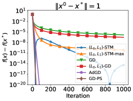
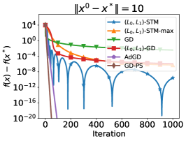
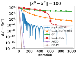
The existing numerical studies already illustrate the benefits of many methods considered in this paper in solving -smooth problems. In particular, the results of numerical experiments with Clip-GD, which is closely related to -GD, GD-PS, and AdGD on training LSTM (Merity et al.,, 2018) and/or ResNet (He et al.,, 2016) models are provided in (Zhang et al., 2020b, ; Loizou et al.,, 2021; Malitsky and Mishchenko,, 2020). Therefore, in our numerical experiments, we focus on a simple -dimensional problem that is convex, -smooth, and provides additional insights to the ones presented in the literature. In particular, we consider function , which is convex, -smooth, but not -smooth as illustrated in Example 1.4. We run (i) with stepsize , (which corresponds to the worst-case smoothness constant on the interval ), (ii) -GD with , , , (iii) -STM with (not supported by our theory) and (iv) with (called -STM-max on the plots), (v) GD-PS, and (vi) AdGD for starting points . The results are reported in Figure 1. In all tests, GD-PS and AdGD show the best results among other methods (which is expected since these methods are the only parameter-free methods). Next, standard GD is the slowest among other methods and slow-downs once we move the starting point further from the optimum, which is also expected since increases and we have to use smaller stepsizes for GD. Finally, let us discuss the behavior of -GD, -STM-max, and -STM. Clearly, it depends on the distance from the starting point to the solution. In particular, when we have , meaning that . In this case, GD and -GD behave similarly to each other, and -STM-max significantly outperforms both of them, which is well-aligned with the derived bounds. However, for and we have and leading to a significant slow down in the convergence of GD and -STM-max. In particular, -GD achieves a similar optimization error to -STM-max for and much better optimization error for . This is also aligned with our theoretical results: when is large and number of iterations is not too large, bound (15) derived for -GD can be better than bound (25) derived for -STM-max. Moreover, for , Figure 1 illustrates well the two-stages convergence behavior of -GD described in Theorem 3.3. Finally, although our theory does not provide any guarantees for -STM with , this method converges faster than -GD for the considered problem but exhibits highly non-monotone behavior.
9 Conclusion and Future Work
In this paper, we derive improved convergence rates for -GD and GD-PS, derive convergence guarantees for the new accelerated method called -STM, and also derive a new result for AdGD in the case of (strongly) convex -smooth optimization. Our results for -GD and GD-PS depend neither on nor on nor on exponential functions of . We also prove new results for the stochastic extensions of -GD and GD-PS in the case of finite sums of functions having a common minimizer.
Nevertheless, several important questions remain open. One of these questions is the lower bounds for the class of (strongly) convex -smooth functions and optimal methods for this class. Next, it is unclear whether the bound (29) derived for AdGD is tight. Finally, it would be interesting to develop stochastic extensions of -GD and GD-PS with strong theoretical guarantees beyond the case of finite sums with shared minimizer.
Acknowledgements
We thank Konstantin Mishchenko for useful suggestions for improving the writing.
References
- Abadi et al., (2016) Abadi, M., Chu, A., Goodfellow, I., McMahan, H. B., Mironov, I., Talwar, K., and Zhang, L. (2016). Deep learning with differential privacy. In Proceedings of the 2016 ACM SIGSAC conference on computer and communications security, pages 308–318.
- Abdukhakimov et al., (2024) Abdukhakimov, F., Xiang, C., Kamzolov, D., and Takáč, M. (2024). Stochastic gradient descent with preconditioned polyak step-size. Computational Mathematics and Mathematical Physics, 64(4):621–634.
- Bartlett et al., (1998) Bartlett, P., Freund, Y., Lee, W. S., and Schapire, R. E. (1998). Boosting the margin: A new explanation for the effectiveness of voting methods. The annals of statistics, 26(5):1651–1686.
- Bauschke et al., (2017) Bauschke, H. H., Bolte, J., and Teboulle, M. (2017). A descent lemma beyond lipschitz gradient continuity: first-order methods revisited and applications. Mathematics of Operations Research, 42(2):330–348.
- Belkin et al., (2019) Belkin, M., Rakhlin, A., and Tsybakov, A. B. (2019). Does data interpolation contradict statistical optimality? In The 22nd International Conference on Artificial Intelligence and Statistics, pages 1611–1619. PMLR.
- Berrada et al., (2020) Berrada, L., Zisserman, A., and Kumar, M. P. (2020). Training neural networks for and by interpolation. In International Conference on Machine Learning.
- Carmon et al., (2021) Carmon, Y., Duchi, J. C., Hinder, O., and Sidford, A. (2021). Lower bounds for finding stationary points ii: first-order methods. Mathematical Programming, 185(1):315–355.
- Chen et al., (2020) Chen, X., Wu, S. Z., and Hong, M. (2020). Understanding gradient clipping in private sgd: A geometric perspective. Advances in Neural Information Processing Systems, 33:13773–13782.
- Chen et al., (2023) Chen, Z., Zhou, Y., Liang, Y., and Lu, Z. (2023). Generalized-smooth nonconvex optimization is as efficient as smooth nonconvex optimization. In International Conference on Machine Learning, pages 5396–5427. PMLR.
- Crawshaw et al., (2022) Crawshaw, M., Liu, M., Orabona, F., Zhang, W., and Zhuang, Z. (2022). Robustness to unbounded smoothness of generalized signsgd. Advances in neural information processing systems, 35:9955–9968.
- Cutkosky and Mehta, (2021) Cutkosky, A. and Mehta, H. (2021). High-probability bounds for non-convex stochastic optimization with heavy tails. Advances in Neural Information Processing Systems, 34:4883–4895.
- Defazio and Bottou, (2019) Defazio, A. and Bottou, L. (2019). On the ineffectiveness of variance reduced optimization for deep learning. Advances in Neural Information Processing Systems, 32.
- Fatkhullin et al., (2023) Fatkhullin, I., He, N., and Hu, Y. (2023). Stochastic optimization under hidden convexity. arXiv preprint arXiv:2401.00108.
- Faw et al., (2023) Faw, M., Rout, L., Caramanis, C., and Shakkottai, S. (2023). Beyond uniform smoothness: A stopped analysis of adaptive sgd. In The Thirty Sixth Annual Conference on Learning Theory, pages 89–160. PMLR.
- Galli et al., (2023) Galli, L., Rauhut, H., and Schmidt, M. (2023). Don't be so monotone: Relaxing stochastic line search in over-parameterized models. In Advances in Neural Information Processing Systems.
- Gasnikov and Nesterov, (2016) Gasnikov, A. and Nesterov, Y. (2016). Universal fast gradient method for stochastic composit optimization problems. arXiv preprint arXiv:1604.05275.
- Goodfellow et al., (2016) Goodfellow, I., Bengio, Y., and Courville, A. (2016). Deep Learning. MIT Press. http://www.deeplearningbook.org.
- Gorbunov et al., (2020) Gorbunov, E., Danilova, M., and Gasnikov, A. (2020). Stochastic optimization with heavy-tailed noise via accelerated gradient clipping. Advances in Neural Information Processing Systems, 33:15042–15053.
- Gorbunov et al., (2021) Gorbunov, E., Danilova, M., Shibaev, I., Dvurechensky, P., and Gasnikov, A. (2021). Near-optimal high probability complexity bounds for non-smooth stochastic optimization with heavy-tailed noise. arXiv preprint arXiv:2106.05958.
- Goujaud et al., (2024) Goujaud, B., Moucer, C., Glineur, F., Hendrickx, J. M., Taylor, A. B., and Dieuleveut, A. (2024). PEPit: computer-assisted worst-case analyses of first-order optimization methods in python. Mathematical Programming Computation, pages 1–31.
- Gower et al., (2021) Gower, R., Sebbouh, O., and Loizou, N. (2021). SGD for structured nonconvex functions: Learning rates, minibatching and interpolation. In International Conference on Artificial Intelligence and Statistics, pages 1315–1323. PMLR.
- Hazan and Kakade, (2019) Hazan, E. and Kakade, S. M. (2019). Revisiting the Polyak step size. In arXiv.
- He et al., (2016) He, K., Zhang, X., Ren, S., and Sun, J. (2016). Deep residual learning for image recognition. In Proceedings of the IEEE conference on computer vision and pattern recognition, pages 770–778.
- Horváth et al., (2022) Horváth, S., Mishchenko, K., and Richtárik, P. (2022). Adaptive learning rates for faster stochastic gradient methods. arXiv preprint arXiv:2208.05287.
- Hübler et al., (2024) Hübler, F., Yang, J., Li, X., and He, N. (2024). Parameter-agnostic optimization under relaxed smoothness. In International Conference on Artificial Intelligence and Statistics, pages 4861–4869. PMLR.
- Jin et al., (2021) Jin, J., Zhang, B., Wang, H., and Wang, L. (2021). Non-convex distributionally robust optimization: Non-asymptotic analysis. Advances in Neural Information Processing Systems, 34:2771–2782.
- Karimireddy et al., (2021) Karimireddy, S. P., He, L., and Jaggi, M. (2021). Learning from history for byzantine robust optimization. In International Conference on Machine Learning, pages 5311–5319. PMLR.
- Koloskova et al., (2023) Koloskova, A., Hendrikx, H., and Stich, S. U. (2023). Revisiting gradient clipping: Stochastic bias and tight convergence guarantees. In International Conference on Machine Learning.
- (29) Li, H., Qian, J., Tian, Y., Rakhlin, A., and Jadbabaie, A. (2024a). Convex and non-convex optimization under generalized smoothness. Advances in Neural Information Processing Systems, 36.
- (30) Li, H., Rakhlin, A., and Jadbabaie, A. (2024b). Convergence of adam under relaxed assumptions. Advances in Neural Information Processing Systems, 36.
- Liang and Rakhlin, (2020) Liang, T. and Rakhlin, A. (2020). Just interpolate. The Annals of Statistics, 48(3):1329–1347.
- Liu et al., (2022) Liu, C., Zhu, L., and Belkin, M. (2022). Loss landscapes and optimization in over-parameterized non-linear systems and neural networks. Applied and Computational Harmonic Analysis, 59:85–116.
- Loizou et al., (2021) Loizou, N., Vaswani, S., Laradji, I. H., and Lacoste-Julien, S. (2021). Stochastic polyak step-size for sgd: An adaptive learning rate for fast convergence. In International Conference on Artificial Intelligence and Statistics, pages 1306–1314. PMLR.
- Mai and Johansson, (2021) Mai, V. V. and Johansson, M. (2021). Stability and convergence of stochastic gradient clipping: Beyond lipschitz continuity and smoothness. In International Conference on Machine Learning, pages 7325–7335. PMLR.
- Malinovsky et al., (2023) Malinovsky, G., Richtárik, P., Horváth, S., and Gorbunov, E. (2023). Byzantine robustness and partial participation can be achieved simultaneously: Just clip gradient differences. arXiv preprint arXiv:2311.14127.
- Malitsky and Mishchenko, (2020) Malitsky, Y. and Mishchenko, K. (2020). Adaptive gradient descent without descent. In International Conference on Machine Learning, pages 6702–6712. PMLR.
- Malitsky and Mishchenko, (2023) Malitsky, Y. and Mishchenko, K. (2023). Adaptive proximal gradient method for convex optimization. arXiv preprint arXiv:2308.02261.
- Merity et al., (2018) Merity, S., Keskar, N. S., and Socher, R. (2018). Regularizing and optimizing LSTM language models. In International Conference on Learning Representations.
- Nemirovski and Yudin, (1983) Nemirovski, A. S. and Yudin, D. B. (1983). Problem Complexity and Method Efficiency in Optimization. A Wiley-Interscience publication. Wiley.
- Nemirovskii and Nesterov, (1985) Nemirovskii, A. S. and Nesterov, Y. E. (1985). Optimal methods of smooth convex minimization. USSR Computational Mathematics and Mathematical Physics, 25(2):21–30.
- Nesterov, (2018) Nesterov, Y. (2018). Lectures on Convex Optimization. Springer.
- Nesterov, (1983) Nesterov, Y. E. (1983). A method for solving the convex programming problem with convergence rate O. In Dokl. akad. nauk Sssr, volume 269, pages 543–547.
- Pascanu et al., (2013) Pascanu, R., Mikolov, T., and Bengio, Y. (2013). On the difficulty of training recurrent neural networks. In International Conference on Machine Learning.
- Patel and Berahas, (2022) Patel, V. and Berahas, A. S. (2022). Gradient descent in the absence of global lipschitz continuity of the gradients. arXiv preprint arXiv:2210.02418.
- Patel et al., (2022) Patel, V., Zhang, S., and Tian, B. (2022). Global convergence and stability of stochastic gradient descent. Advances in Neural Information Processing Systems, 35:36014–36025.
- Polyak, (1987) Polyak, B. (1987). Introduction to Optimization. Optimization Software.
- Polyak, (1964) Polyak, B. T. (1964). Some methods of speeding up the convergence of iteration methods. Ussr computational mathematics and mathematical physics, 4(5):1–17.
- Robbins and Monro, (1951) Robbins, H. and Monro, S. (1951). A stochastic approximation method. The annals of mathematical statistics, pages 400–407.
- Sadiev et al., (2023) Sadiev, A., Danilova, M., Gorbunov, E., Horváth, S., Gidel, G., Dvurechensky, P., Gasnikov, A., and Richtárik, P. (2023). High-probability bounds for stochastic optimization and variational inequalities: the case of unbounded variance. In International Conference on Machine Learning.
- Shalev-Shwartz and Ben-David, (2014) Shalev-Shwartz, S. and Ben-David, S. (2014). Understanding machine learning: From theory to algorithms. Cambridge university press.
- Sutskever et al., (2013) Sutskever, I., Martens, J., Dahl, G., and Hinton, G. (2013). On the importance of initialization and momentum in deep learning. In International conference on machine learning, pages 1139–1147. PMLR.
- Takezawa et al., (2024) Takezawa, Y., Bao, H., Sato, R., Niwa, K., and Yamada, M. (2024). Polyak meets parameter-free clipped gradient descent. arXiv preprint arXiv:2405.15010.
- (53) Vaswani, S., Bach, F., and Schmidt, M. (2019a). Fast and faster convergence of sgd for over-parameterized models and an accelerated perceptron. In The 22nd international conference on artificial intelligence and statistics, pages 1195–1204. PMLR.
- (54) Vaswani, S., Mishkin, A., Laradji, I., Schmidt, M., Gidel, G., and Lacoste-Julien, S. (2019b). Painless stochastic gradient: Interpolation, line-search, and convergence rates. Advances in neural information processing systems, 32.
- Wang et al., (2023) Wang, B., Zhang, H., Ma, Z., and Chen, W. (2023). Convergence of adagrad for non-convex objectives: Simple proofs and relaxed assumptions. In The Thirty Sixth Annual Conference on Learning Theory, pages 161–190. PMLR.
- Wang et al., (2022) Wang, B., Zhang, Y., Zhang, H., Meng, Q., Ma, Z.-M., Liu, T.-Y., and Chen, W. (2022). Provable adaptivity in adam. arXiv preprint arXiv:2208.09900.
- (57) Zhang, B., Jin, J., Fang, C., and Wang, L. (2020a). Improved analysis of clipping algorithms for non-convex optimization. In Advances in Neural Information Processing Systems.
- Zhang et al., (2021) Zhang, C., Bengio, S., Hardt, M., Recht, B., and Vinyals, O. (2021). Understanding deep learning (still) requires rethinking generalization. Communications of the ACM, 64(3):107–115.
- (59) Zhang, J., He, T., Sra, S., and Jadbabaie, A. (2020b). Why gradient clipping accelerates training: A theoretical justification for adaptivity. In International Conference on Learning Representations.
- (60) Zhang, J., Karimireddy, S. P., Veit, A., Kim, S., Reddi, S., Kumar, S., and Sra, S. (2020c). Why are adaptive methods good for attention models? In Advances in Neural Information Processing Systems.
- Zhao et al., (2021) Zhao, S.-Y., Xie, Y.-P., and Li, W.-J. (2021). On the convergence and improvement of stochastic normalized gradient descent. Science China Information Sciences, 64:1–13.
Appendix A Examples of -Smooth Functions
Example A.1 (Power of Norm).
Let , where is a positive integer. Then, is convex and -smooth. Moreover, is not -smooth for .
Proof.
Convexity of follows from convexity and monotonicity of for and convexity of , since . To show -smoothness, we compute gradient and Hessian of :
Therefore,
which implies
If , then we have . If , then
where . For we have and . For we have , which gives . Putting two cases together, we get
that is equivalent to -smoothness (Chen et al.,, 2023, Theorem 1). Non-smoothness of for follows from the unboundedness of in this case. ∎
Example A.2 (Exponent of the Inner Product).
Function for some is convex, -smooth, but not -smooth for any .
Proof.
Let us compute the gradient and Hessian of :
Clearly , meaning that is convex. Moreover,
that is equivalent to -smoothness (Chen et al.,, 2023, Theorem 1). When function has unbounded Hessian, i.e., is not -smooth for any in this case. ∎
Example A.3 (Logistic Function).
Consider logistic function: , where is some vector. Function is -smooth with and .
Proof.
The gradient and the Hessian of equal
Moreover,
This leads to
implying that for all . This condition is equivalent to -smoothness (Chen et al.,, 2023, Theorem 1). ∎
Appendix B Proof of Lemma 2.2
Lemma B.1 (Lemma 2.2).
Proof.
Next, we will prove (35) and (36) under Assumptions 1.1 and 1.3. The proof follows similar steps to the one that holds for standard -smoothness (i.e., cocoercivity of the gradient) (Nesterov,, 2018):
That is, for given we consider function . This function is differentiable and . Moreover, for any we have
| (37) |
Next, for given and for any we define function as . Then, by definition of , we have , , and . Therefore, using Newton-Leibniz formula, we derive
that implies
| (38) |
To proceed, we will need the following inequality:
| (39) | |||||
Using the above bound and (38) with , we derive
Taking into account that is an optimum for () and the definition of , we get the following inequality from the above one:
which is equivalent to
Therefore, we established (35). Moreover, by swapping and in the above inequality, we also get
To get (36), it remains to sum the above two inequalities. ∎
Appendix C Missing Proofs for -GD
Lemma C.1 (Lemma 3.1: monotonicity of function value).
Let Assumption 1.3 hold. Then, for all the iterates generated by -GD with , satisfy
| (40) |
Proof.
Lemma C.2 (Lemma 3.2: monotonicity of gradient norm).
Proof.
For convenience, we introduce the following notation: for all . Since
the assumptions for the second part of Lemma 2.2 are satisfied for and , and inequality (11) implies
where in the second line we use . Multiplying both sides by and rearranging the terms, we get
which is equivalent to
We notice that and since . Moreover, due to the convexity of we also have . Therefore, we have
Together with (C), the above inequality implies
which is equivalent to (42). ∎
Theorem C.3 (Theorem 3.3).
Proof.
We start by expanding the squared distance to the solution:
| (47) | |||||
To continue the derivation, we consider two possible cases: or .
Case 1: . In this case, we have
| (48) | |||
| (49) |
Plugging the above inequalities in (47), we continue the derivation as follows:
| (50) | |||||
We notice that if , then, in view of Lemma 3.2, we also have for all . Therefore, (50) implies
| (51) |
Since , should be bounded as , which gives (14). We denote for the set . Therefore, in view of (51) and non-negativity of the squared distance, is bounded as .
Case 2: . In this case, we have
| (52) |
implying that
| (53) |
Moreover, since the norm of the gradient is non-increasing along the trajectory of -GD (Lemma 3.2), implies that . Therefore, we can sum up inequalities (53) for , rearrange the terms, and get
Finally, we take into account that for , we have :
| (54) |
It remains to notice that Lemma 3.1 implies . Together with the above inequality, it implies the first part (15). To derive the second part of (15), it remains to notice that for the right-hand side of (54) as a function of attains its maximum at . Indeed, the derivative of function
equals
Since , we have , i.e., is a decreasing function of , meaning that
which gives (45).
Appendix D Missing Proofs for Gradient Descent with Polyak Stepsizes
Theorem D.1 (Theorem 4.1).
Let Assumptions 1.1 with and 1.3 hold. Then, the iterates generated by GD-PS satisfy the following implication:
| (56) |
Moreover, the output after steps the iterates satisfy
| (57) |
where , , and if , it holds that
| (58) |
where is such that . In particular, for inequality is guaranteed and
| (59) |
In addition, if and , then
| (60) |
Proof.
As for -GD, we start by expanding the squared distance to the solution:
| (61) | |||||
To continue the derivation, we consider two possible cases: or .
Case 1: . In this case, inequalities (48) and (49) hold and the derivation from (61) can be continued as follows:
| (62) | |||||
which gives (56).
Case 2: . In this case, inequality (52) holds and we have
| (63) |
Next, we introduce the set of indices of size . In view of the above derivations, if , inequality (62) holds, and if , inequality (63) is satisfied. Therefore, unrolling the pair of inequalities (62) and (63), we get
which is equivalent to (57). Therefore, if , set is non-empty and the above inequality implies
where is such that . Moreover, since the left-hand side of (57) is non-negative, we have . Therefore, for inequality is guaranteed as well as (58). Finally, to derive (59), we consider the right-hand side of (58) as a function of :
The derivative of this function equals
Since , we have , i.e., is a decreasing function of . Therefore, since , we have that
Appendix E Missing Proofs for -Similar Triangles Method
Lemma E.1 (Lemma E.1 from (Gorbunov et al.,, 2020)).
Let sequences and be defined as follows:
Then, for all
| (65) | |||||
| (66) |
Lemma E.2 (Lemma 5.1).
Proof.
The proof follows the one of Lemma F.4 from (Gorbunov et al.,, 2020). From the update rule, we have and
The update rules for and imply
| (69) |
Moreover, to proceed, we will need the following upper-bound:
| (70) | |||||
Using these formulas, we continue the derivation as follows:
| (71) | |||||
Next, using the definition of and , we get
| (72) |
Combining the established inequalities, we obtain
which can be rewritten as
Summing up the above inequality for and using , , and new notation , we derive
which finishes the proof. ∎
Theorem E.3 (Theorem 5.2).
Proof.
Let us prove by induction that for all . For , the statement is trivial. Next, we assume that the statement holds for and derive that it also holds for . Indeed, from Lemma 5.1 we have
| (75) | |||||
implying that . That is, we proved that for all , i.e., the sequence stays in . Since , is a convex combination of and , is a convex combination of and , we also have that sequences and stay in , which can be formally shown using an induction argument. Therefore, we can upper-bound for all as follows
| (76) | |||||
Moreover, from (75) we also have
which finishes the proof. ∎
Appendix F Missing Proofs for Adaptive Gradient Descent
F.1 Proof of Theorem 6.1
The key lemma about the convergence of AdGD holds for any convex function regardless of the smoothness properties.
Lemma F.1 (Lemma 1 from Malitsky and Mishchenko, (2020)).
In particular, the above lemma implies boundedness of and , which allows us to get the upper bound on the gradient norm (26) and a lower bound for as stated in the paragraph before Theorem 6.1. For completeness, we provide the proof of this theorem below.
Theorem F.2 (Theorem 6.1).
Proof.
The proof follows almost the same lines as the proof from (Malitsky and Mishchenko,, 2020). Telescoping inequality (77), we get
| (79) |
Since by definition of , we conclude that the term in the second line of the above inequality is non-negative. Therefore, for any we have
| (80) | |||||
| (81) |
Using Jensen’s inequality in (F.1), we derive
where
| (82) | |||||
| (83) | |||||
| (84) |
Thus, we have
| (85) |
Next, we notice that for any
Since , we have . Moreover, for we have either or . Therefore, by induction we can prove that
| (86) |
that implies
Therefore, we have
which is equivalent to (78) when . ∎
F.2 Proof of Theorem 6.2
Lemma F.3.
Proof.
The proof is almost identical to the one from (Malitsky and Mishchenko,, 2020) and starts as the standard proof for GD:
Introducing , we rewrite the above inequality as
| (88) | |||||
Next, we transform similarly to the original proof:
| (89) | |||||
Next, we apply Cauchy-Schwarz inequality, the definition of with , and Young’s inequality to estimate the first inner-product in the right-hand side:
| (90) |
Then, using the convexity of , we handle the second inner product from the right-hand side of (89):
| (91) |
Plugging (F.2) and (F.2) in (89), we get
Finally, using the above upper bound for in (88), we obtain
Rearranging the terms, we derive (87). ∎
The above lemma implies not only the boundedness of the iterates but also the boundedness of for .
Corollary F.4.
Using the above results, we derive the following theorem.
Theorem F.5 (Theorem 6.2).
Proof.
Since we will use -smoothness only between two consecutive iterates , for the sake of brevity, we unify the notation for Assumptions 1.2 and 1.3 as
| (97) |
where , if Assumption 1.2 holds (follows from the definition), and , if Assumption 1.3 holds (follows from (6) and (93)).
Since666In practice it is sufficient to take . , we have . Next, for we have either or . For convenience of the analysis of these two options, we let be the set of indices such that and .
Option 1: . Then, by definition of , there exists index such that , for all , , and , i.e., belongs to some sub-sequence of indices such that Option 1 holds. Following exactly the same steps as in the derivation of (86), we conclude that for any . Since for all , we get that for , meaning that for larger than we have . Putting all together, we conclude that
| (98) |
To continue the proof, we split the set of indices into three disjoint sets defined as follows: ,
, and . Then, taking into account the lower bounds (98) and (99), we have
Therefore, we can lower bound the sum of stepsizes as follows:
| (100) | |||||
Since (see the definition in (84)) we have from (85) and the above lower bound on that
which gives
| (101) |
when Assumption 1.3 holds, and
when Assumption 1.2 is satisfied. In particular, we derived (95) under Assumption 1.3 holds, and when , we have , which in combination with (101) implies (96).
∎
F.3 Convergence in the Strongly Convex Case
To show an improved result in the strongly convex case ( in Assumptions 1.1), we consider Algorithm 4 with more a more conservative stepsize selection rule:
| (102) |
For these stepsizes, Lemma F.3 holds as well. However, in contrast to the convex case, we will use Assumption 1.2 instead of Assumption 1.3. The key reason for this is that we need to use (10) for and that not necessarily satisfy (9). In contrast, inequality (10) holds for any under the Assumption 1.2 and convexity.
Theorem F.6.
Proof.
The proof follows the one from (Malitsky and Mishchenko,, 2020). First of all, we note that the stricter inequality is not used in the derivation of Lemma F.3. Therefore, Lemma F.3 holds as well as Corollary F.4. Next, we make certain steps in the analysis tighter to use the fact that . Strong convexity implies
| (105) |
and . The latter implies that for . Since Lemma 2.2 holds under Assumption 1.2 with and without condition (9), and bound holds, we have
| (106) | |||||
Convex combination of (105) and (106) with , which will be specified latter, gives
Using the above inequality instead of convexity and keeping the rest of the proof of Lemma F.3 as is with omitted terms, we get an analog of (77):
where the first inequality follows from provided by the new condition on . Thus, we have contraction in every term: in the first, in the second and in the last one. We bound the third term as using for both terms in the denominator. Taking , which is the root of , we bound the second term as . Therefore, for we have
| (107) |
The final step of the proof is unrolling the recursion for Lyapunov function . Following the proof of Theorem F.5, we have that
| (108) |
with , which differs from defined in the convex case due to the new condition on . Therefore, by repeating all the steps from the proof of (100), we obtain
| (109) |
Next, we bound the product that arises during recursion unrolling by using the relation between the geometric mean and the arithmetic mean:
| (110) | |||||
Finally, we combine (107) and (110) and get
Moreover, when , we have , which in combination with the above inequality implies (104).
∎
Appendix G Stochastic Extensions: Missing Proofs and Details
G.1 -Stochastic Gradient Descent
Theorem G.1 (Theorem 7.2).
Let Assumption 7.1 hold. Then, the iterates generated by -SGD with , after iterations satisfy
| (111) |
Proof.
Similarly to the deterministic case, we start by expanding the squared distance , which is a common minimizer for all :
| (112) | |||||
As before, we consider two possible cases: or .
Case 1: . In this case, we have
| (113) | |||
| (114) |
Plugging the above inequalities in (112), we continue the derivation as follows:
| (115) | |||||
Case 2: . In this case, we have
| (116) |
implying that
| (117) |
To combine (115) and (117), we introduce event for given and indicator of event as , i.e., for given , we have if , and if . Then, inequalities (115) and (117) can be unified as follows:
Let us denote the expectation conditioned on as . Taking from the both sides of the above inequality, we derive
where . Note that is a random variable itself. Nevertheless, if , it means that for at least one we have for given . Therefore, either or . Moreover, when , we have for given . Putting all together, we continue as follows:
Taking full expectation from the above inequality and telescoping the result, we get
Since is not greater than
, we also have
Dividing both sides by , we obtain (111). ∎
G.2 Stochastic Gradient Descent with Polyak Stepsizes
Theorem G.2 (Theorem 7.3).
Let Assumption 7.1 hold. Then, the iterates generated by SGD-PS after iterations satisfy
| (118) |
Proof.
Similarly to the deterministic case, we start by expanding the squared distance , which is a common minimizer for all :
| (119) | |||||
As before, we consider two possible cases: or .
Case 1: . In this case, inequalities (113) and (114) hold and the derivation from (119) can be continued as follows:
| (120) | |||||
which gives (56).
Case 2: . In this case, inequality (116) holds and we have
| (121) |
To combine (120) and (121), we introduce event for given and indicator of event as , i.e., for given , we have if , and if . Then, inequalities (120) and (121) can be unified as follows:
Let us denote the expectation conditioned on as . Taking from the both sides of the above inequality, we derive
where . Note that is a random variable itself. Nevertheless, if , it means that for at least one we have for given . Therefore, either or . Moreover, when , we have for given . Putting all together, we continue as follows:
Taking full expectation from the above inequality and telescoping the result, we get
Since is not greater than
, we also have
Dividing both sides by , we obtain (118). ∎