Sparse-to-Dense LiDAR Point Generation
by LiDAR-Camera Fusion for 3D Object Detection

Abstract

Accurately detecting objects at long distances remains a critical challenge in 3D object detection when relying solely on LiDAR sensors due to the inherent limitations of data sparsity. To address this issue, we propose the LiDAR-Camera Augmentation Network (LCANet), a novel framework that reconstructs LiDAR point cloud data by fusing 2D image features, which contain rich semantic information, generating additional points to improve detection accuracy. LCANet fuses data from LiDAR sensors and cameras by projecting image features into the 3D space, integrating semantic information into the point cloud data. This fused data is then encoded to produce 3D features that contain both semantic and spatial information, which are further refined to reconstruct final points before bounding box prediction. This fusion effectively compensates for LiDAR’s weakness in detecting objects at long distances, which are often represented by sparse points. Additionally, due to the sparsity of many objects in the original dataset, which makes effective supervision for point generation challenging, we employ a point cloud completion network to create a complete point cloud dataset that supervises the generation of dense point clouds in our network. Extensive experiments on the KITTI and Waymo datasets demonstrate that LCANet significantly outperforms existing models, particularly in detecting sparse and distant objects.

I Introduction

LiDAR sensors are among the most widely utilized devices for capturing three-dimensional (3D) representations of real-world environments. However, the 3D point clouds generated by LiDAR sensors often contain sparse point distributions, which can result in insufficient semantic information for object identification. This sparsity arises because the device emits laser pulses in a circular pattern with discrete angular intervals, leading to dense point captures near the sensor and sparse point captures at farther distances. Consequently, this sparsity hinders the accurate recognition of distant objects, degrading performance in 3D detection tasks. Fig. 2 presents the distribution of points by range and the detection results using the 3D object detector PointPillars [1]. Objects in close proximity to the ego vehicle typically have well-formed point clouds, making them easier to identify. In contrast, objects located at greater distances are represented by sparser point clouds, leading to challenges in detection. This suggests that by making sparse points denser and ensuring they retain their original shape, detection performance can be improved, thereby addressing the inherent limitations of LiDAR sensors.

Several approaches, including [2, 3, 4], have focused on generating additional points within regions of interest (RoIs) to enhance spatial and contextual information, thereby improving the accuracy of 3D object detection performance and addressing the sparsity and incompleteness of point clouds. However, these methods rely solely on 3D point clouds, which can lead to the misclassification of sparse background points as foreground objects during the point cloud completion process, as shown in Fig. 1. Generating points without incorporating visual information, where non-object points are mistakenly identified as obstacles or objects, can be particularly dangerous for autonomous driving and robotics, as misidentifying noise points as obstacles may lead to incorrect decision-making and hazardous situations.

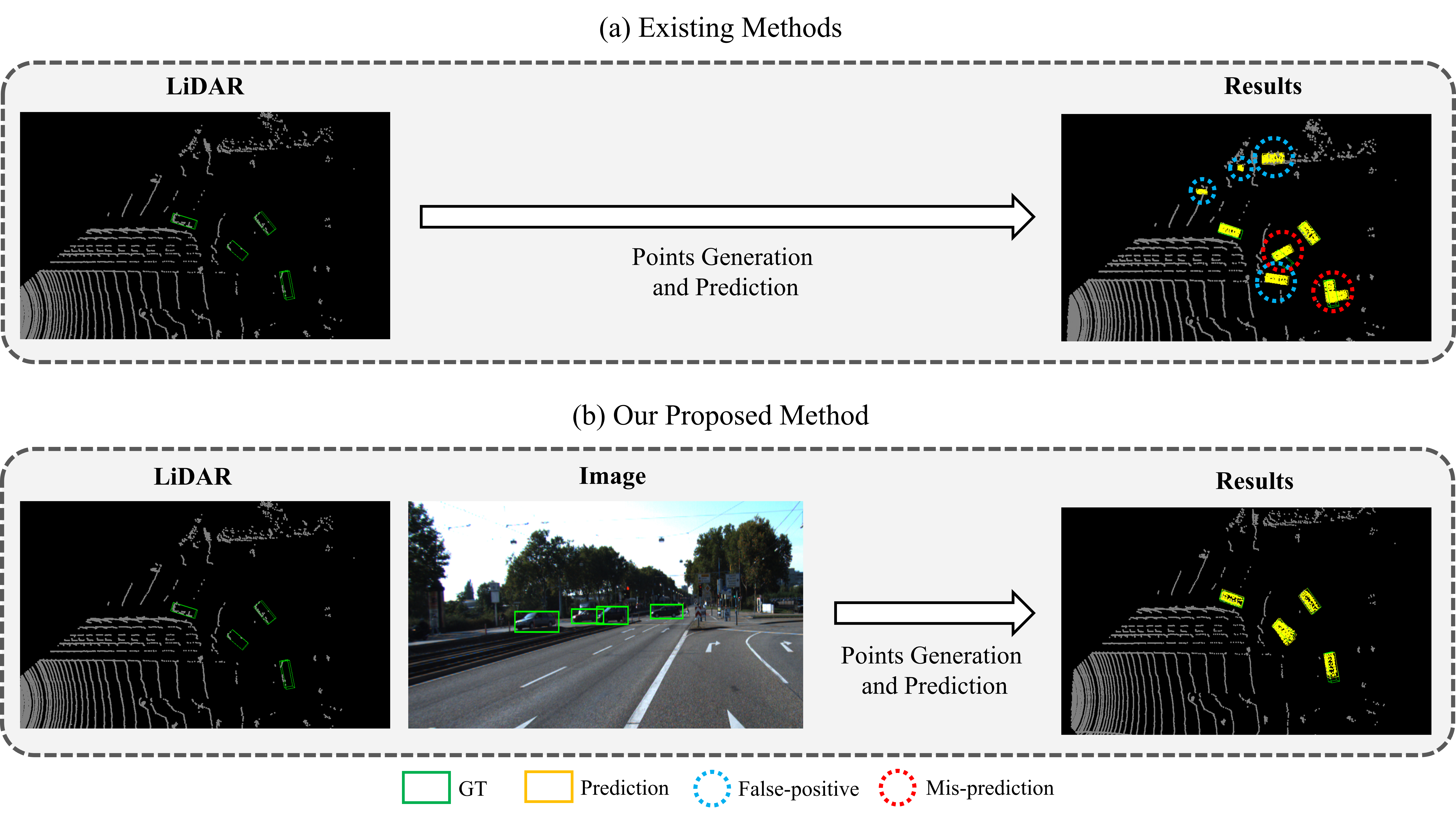
Figure 1: Points generation and detection results. Our proposed method (b) utilizing both LiDAR and images generates points and detects bounding boxes more accurately for sparse objects compared to methods that rely solely on 3D point clouds (a), with the bounding box axes being especially well-aligned to the ground truth (GT) boxes, and with fewer false positives.

To address these challenges, we propose the LiDAR-Camera Augmentation Network (LCANet), which integrates 2D image features with RoI grid-pooled features to generate semantically enriched points corresponding to objects visible in the image, thereby enhancing the overall quality of the point cloud. Initially, raw LiDAR points are decorated with image features using the Semantic Points Encoding (SPE) module, voxelized, and then fed into a 3D backbone network to extract multi-level voxel features. These voxel features are subsequently mapped to bird’s-eye view (BEV) space and processed by a region proposal network (RPN) to generate initial bounding box predictions. Next, the Cross-Modal Feature Fusion network (CMFF) fuses features from different modalities through 3D RoI grid pooling [5], 2D RoI grid pooling, and RoI Align [6], aggregating multi-level voxel and image features surrounding these grids. The RoI Point Generation network (RPG) generates additional points using a transformer encoder, and the SPE module is employed once more to provide additional image features to the generated points, preventing the generation of misaligned points. These generated points are then encoded using a point encoder, followed by final bounding box refinement and the calculation of a confidence score. Fig. 1 shows the point generation results of LiDAR-only methods [4] compared to our method, which yields more precise point generation and box predictions with fewer false positives. Our contributions are as follows:

• Our proposed LCANet integrates 2D image features with 3D LiDAR data to generate additional points, improving detection performance for distant and sparse objects.

• We introduce a new paradigm of feature fusion, where additional points are generated by combining features from both images and LiDAR to overcome the inherent limitations of LiDAR.

• LCANet demonstrates superior performance over existing points generation models, particularly in detecting distant objects, as validated by experiments on the KITTI and Waymo datasets.

Extensive experiments conducted on the KITTI [7] and Waymo Open Dataset (WOD) [8] datasets demonstrate the effectiveness of our proposed LCANet compared to other point generation models. Our ablation studies and qualitative results show that fusing LiDAR and camera features while generating points significantly improves overall detection performance, particularly for objects located farther from the ego vehicle.

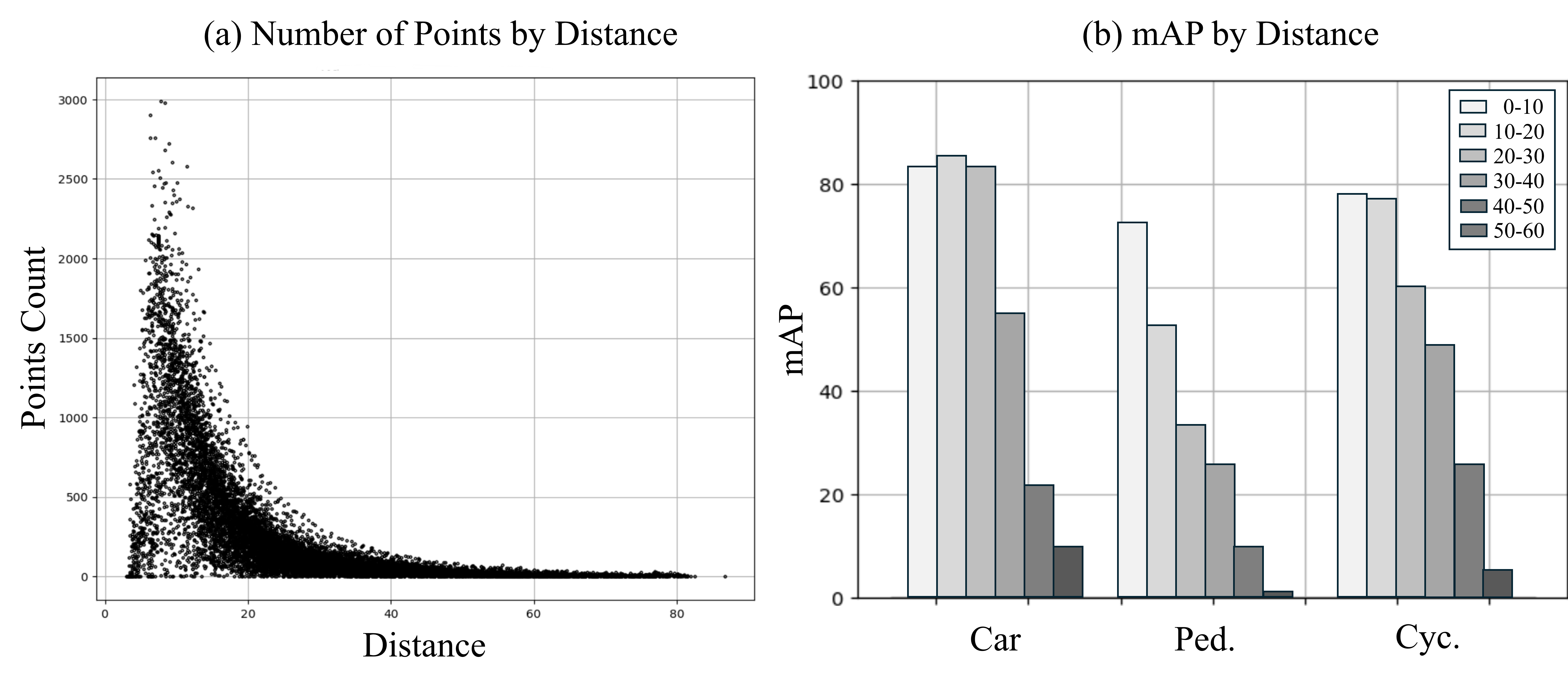
Figure 2: (a) The LiDAR points on each object become dramatically sparser as objects are located farther from the ego-vehicle. Also, (b) detection accuracy decreases for these objects for all classes, accordingly. Note that we use PointPillars [1] with KITTI dataset.

II Related Work

3D Object Detection. 3D object detection involves localizing objects within a three-dimensional scene, typically represented as point cloud data. Point-based 3D object detectors [9, 10, 11] extract features directly from raw points and detect 3D objects based on these features. Grid-based methods address some of the computational challenges by dividing the 3D scene into a grid structure, such as voxels, with [12, 5, 13, 1] being prominent examples of this approach. These methods partition the scene into voxels or pillars, and process the results with 2D or 3D convolution layers. Some works, such as [14, 15], combine both point-based and voxel-based methods. For the sensor fusioning area, early research efforts [16, 17] explored fusing camera and LiDAR data at an early stage of the model by decorating points with semantic features derived from images. Other studies, such as [18, 19], demonstrate significant improvements by concatenating features extracted from different modalities, rather than decorating points at the input stage. In contrast, more recent approaches [20, 21, 22, 23, 24] propose fusion methods based on the bird’s-eye view (BEV) space, using LSS [25] to project 2D features into BEV space with dense semantic signals and fuse them with 3D features.

Point Generation for 3D Object Detection. In raw point-based methods, [2] and [3] incorporate points within regions of interest (RoI) to generate dense point clouds, providing supplementary spatial supervision for 3D object detection. Specifically, [2] employs a point cloud completion network [26] to complete the point cloud. Similarly, [4] generates additional points using a GCN-based [27] point cloud completion network. It utilizes farthest point sampling (FPS) for downsampling within the RoIs and generates multi-resolution feature maps [10] to reconstruct the missing parts of the point cloud, all while preserving the original points’ spatial structure. Meanwhile, [4] utilizes RoI-pooled features rather than raw point features within the RoIs. This method first pools multi-scale voxel features of the RoIs from the 3D backbone and subsequently generates additional points that encapsulate more contextual information surrounding the RoIs. However, these methods exclusively rely on 3D point clouds, where sparse background points may be misidentified as foreground objects, leading to erroneous completions. In contrast, our proposed method LCANet captures richer semantic information by incorporating camera image features, which facilitate the generation of semantically meaningful points.

III LiDAR-Camera Augmentation Network

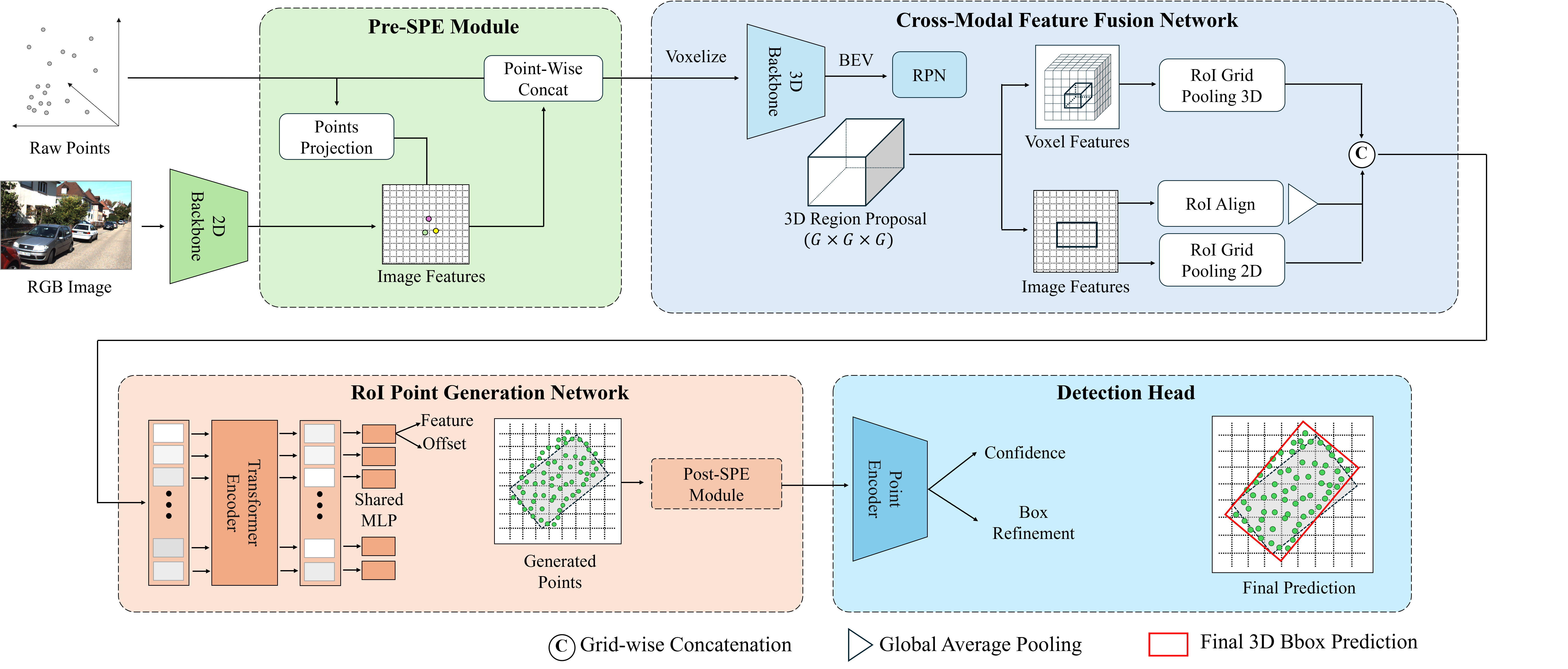
Figure 3: An overview of our proposed LCANet architecture, which consists of four main modules: (i) Semantic Points Encoding (SPE), which decorates LiDAR points with visual semantic features; (ii) Cross-modal Feature Fusion (CMFF), which generates 3D region proposals and extracts camera-LiDAR fused features; (iii) RoI Points Generation, which generates sparse-to-dense LiDAR point clouds for each object; and (iv) Detection Head.

III-A Semantic Points Encoding (SPE)

LiDAR-only detectors often generate false positive and false negative proposals in regions with sparse points due to the lack of semantic priors. Inspired by works such as [17, 16], which demonstrated significant improvements in 3D object detection by augmenting points with semantic priors or image features, we project 3D points onto the image and merge the corresponding image features with the 3D point features for joint embedding. First, we extract image features using a Swin-Transformer [28] and a Feature Pyramid Network (FPN) [29]. The Semantic Points Encoding (SPE) module then maps raw LiDAR points into the image feature space using a calibration matrix. Bilinear interpolation is then employed to extract image features at these projected points and these interpolated features are subsequently concatenated with corresponding points’ features, followed by multilayer perceptrons (MLPs) for channel reduction, thereby enriching each point with semantic information. As a result, the semantic points can generate more semantically accurate region proposals. Additionally, SPE module is utilized in the final step of point generation to incorporate semantic information into the detection process.

III-B Cross-modal Feature Fusion (CMFF)

Region Proposal Generation. Most recent 3D detectors [14, 15, 5, 13, 4] initialize their backbone networks with SECOND [13], leveraging its ability to efficiently generate multi-level voxel features using a sparse convolutional network. The points encoded with our SPE module are voxelized, and features are extracted using SECOND [13]. These features are then compressed along the horizontal axis to produce a bird’s-eye view (BEV) feature map. Directly generating points and predicting from this BEV feature map may be unfeasible due to the lack of spatial information. Therefore, this BEV feature map is subsequently fed into a region proposal network (RPN) to generate initial bounding box predictions. These boxes are further refined using our main modules with points generation.

Feature Extraction and Fusion. Initially, region proposals generated by the RPN are subdivided into $G\times G\times G$ subvoxels, with the centers of these subvoxels serving as grid points. The voxel features surrounding these grid points are aggregated using the approach outlined in Voxel-RCNN [5]. Specifically, the grid feature $f_{g_{i}}^{V}$ is computed by aggregating the features of sampled voxels $\{v_{i}^{1},v_{i}^{2},\dots,v_{i}^{K}\}$ within the vicinity of the grid point $g_{i}$ through the PointNet++ [10] module:

$$f_{g_{i}}^{V}=\texttt{MaxPool}\left\{\texttt{MLP}\left([v_{i}^{k}-g_{i};f_{v_{i}^{k}}]\right)\right\}_{k=1}^{K},$$

where $f_{v_{i}^{k}}$ denotes the voxel features corresponding to the voxel $v_{i}^{k}$, and $v_{i}^{k}-g_{i}$ represents the relative coordinates from grid point $g_{i}$ to voxel $v_{i}^{k}$.

Images contain rich contextual information that is often absent in LiDAR point clouds, making it crucial to capture this information. Each $G\times G\times G$ grids are projected onto the image using calibration matrices and image features are bilinear interpolated on theses points to capture local grid image features $f_{g_{i}}^{I}$. In addition, inspired by methods for generating 2D bounding boxes on the KITTI dataset [7, 19], we project the eight corners of the 3D region proposals onto the image plane using calibration matrices, as shows as Fig. 4. This projection yields eight corner points on the image, from which a 2D bounding box can be derived. To form the bounding box $b_{img}$, we simply select the minimum and maximum values of the $x$ and $y$ coordinates from the projected corners to determine the four outermost corners. Since the initial region proposals may not precisely align with the ground truth (GT) 2D bounding boxes, they require refinement. Enlarging the projected 2D bounding boxes ensures that the GT bounding box is contained within the enlarged box, thereby capturing the relevant features of the objects. Due to the computational cost to capture all features of projected boxes, we utilize RoI Align [6] to efficiently obtain image bbox features $f^{B}$. Finally, $f_{g_{i}}^{V}$, $f_{g_{i}}^{I}$ and $f^{B}$ are concatenated followed by channel reduction to generate fused feature $f_{g_{i}}^{Fus}$, which is written as:

$${f}_{g_{i}}^{Fus}=\texttt{MLP}\left([f_{g_{i}}^{V};f_{g_{i}}^{I};f^{B}]\right)$$ (1)

III-C RoI Points Generation

We follow the same process of generating additional points [4]. However, previous methods [2, 3, 4] only extract features from only LiDAR point derived methods, our method can give more semantic information with the SPE module and CMFF network. However, these fused grid features lack interaction between each others. Therefore, Transformer encoder [30] is used to refine the fused features to capture long-range dependencies between grids of RoIs and can be written as: $\tilde{f}_{g_{i}}^{Fus}=\mathcal{T}(f_{g_{i}}^{Fus},\delta_{g_{i}})$, where $\mathcal{T}$ is the Transformer encoder [30]. Positional encoding is generated with feed-forward network (FFN) and can be formulated as $\delta_{g_{i}}=\texttt{FFN}([g_{i}-\mathbf{r}^{c};g_{i}-\mathbf{r}^{1};g_{i}-\mathbf{r}^{2};\cdots;g_{i}-\mathbf{r}^{8}])$, where $\mathbf{r}^{c}$ is the center and $\mathbf{r}^{1,2,\cdots,8}$ are the eight corners of the 3D bounding box. Finally, MLPs generate points’ semantic features and offsets from the center of the grid $g_{i}$: i.e., $[\mathbf{o}_{i};f^{S}_{\mathbf{p}_{i}}]=\texttt{MLP}(\tilde{f}_{\mathbf{g}_{i}}^{Fus}).$.

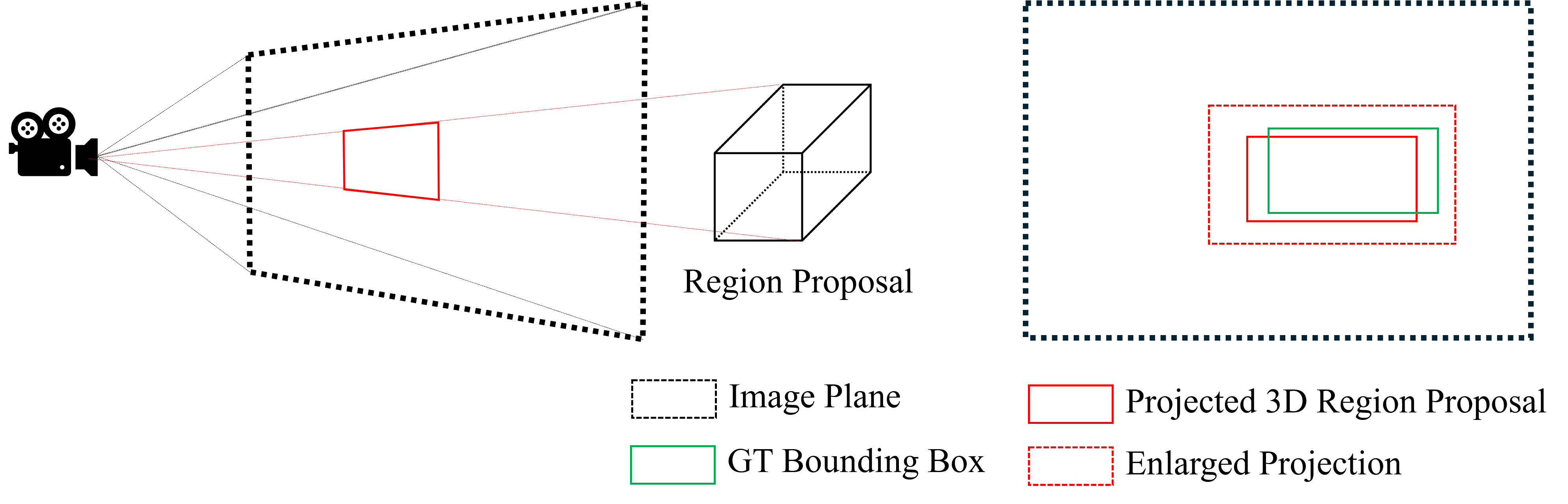
Figure 4: We use enlarged (or padded) projections of 3D region proposals onto the image plane for our RoI point generation to deal with estimation errors in region proposals.

The offsets of the points from the grid centers are geneated, therefore, actual point’s coordinates $\mathbf{p}_{i}=(x_{i},y_{i},z_{i})$ are calculated as $\mathbf{g}_{i}+\mathbf{o}_{i}$. In addition, foreground scores $s_{i}$ for generated points are calculated by MLPs and a sigmoid function $\sigma$, which can be written as $\mathbf{s}_{i}=\sigma(\texttt{MLP}(f^{\text{S}}_{\mathbf{p}_{i}})).$

To optimize, we minimize $\mathcal{L}_{\text{RPG}}$ = $\mathcal{L}_{\text{score}}$ + $\mathcal{L}_{\text{offset}}$. $\mathcal{L}_{\text{offset}}$ ensures that the generated points are geometrically closer to the complete points of objects. We use Chamfer distance described as follows:

$$\mathcal{L}_{\text{offset}}=\frac{1}{N_{p}}\sum_{r}\left(\frac{1}{|\mathbf{S}_{1}|}\sum_{\mathbf{x}\in\mathbf{S}_{1}}\min_{\mathbf{y}\in\mathbf{S}_{2}}\|\mathbf{x}-\mathbf{y}\|_{2}^{2}\right.\\ \left.+\frac{1}{|\mathbf{S}_{2}|}\sum_{\mathbf{y}\in\mathbf{S}_{2}}\min_{\mathbf{x}\in\mathbf{S}_{1}}\|\mathbf{y}-\mathbf{x}\|_{2}^{2}\right)$$ (2)

where $N_{p}$ is the number of positive proposals, and $\mathbf{S}_{1}$ and $\mathbf{S}_{2}$ represent the generated points and the complete object points of the $r$-th foreground proposal, $r=1,2,\cdots,N_{p}$.

Further, $\mathcal{L}_{\text{score}}$ ensures that the generated points reside within the ground truth (GT) bounding boxes. The FPS algorithm [10] is used to sample the generated points and reduce computational costs. $\mathcal{L}_{\text{score}}$ can be described as follows:

$$\mathcal{L}_{\text{score}}=-\frac{1}{N_{s}}\sum_{j}\left((1-s_{j})^{\gamma}\log s_{j}\right),$$ (3)

where $N_{s}$ is the number of sampled points.

III-D Detection Head

To effectively capture the local spatial information of the generated points, these points are first transformed into the canonical space. Nonetheless, it is noteworthy that the canonical transformation may lead to a loss of global context. To mitigate this, the depth $d_{i}=\sqrt{x_{i}^{2}+y_{i}^{2}+z_{i}^{2}}$ is incorporated into the feature set [11]. Additionally, the point score $s_{i}$ is appended to the feature vector to quantify the significance of each point. The MLPs are then applied to extract canonical features from the transformed points, as described by the following equation:

$$f^{\text{C}}_{\mathbf{p}_{i}}=\texttt{MLP}\left(\left[x_{i}^{c},y_{i}^{c},z_{i}^{c},d_{i},s_{i}\right]\right).$$ (4)

where $(x_{i}^{c},y_{i}^{c},z_{i}^{c})$ are the coordinates obtained from the canonical transformation, which is performed based on region proposal prediction. Since generated points may lose detailed semantic features as the network goes deeper, we utilize our SPE module that produces generated image features $f^{\text{I}}_{\mathbf{p}_{i}}$ before feeding them into the point encoder to ensure that the generated points are enriched once more time, providing them with enhanced semantic meaning. Subsequently, the spatial features $f^{\text{C}}_{\mathbf{p}_{i}}$ and semantic features $f^{\text{S}}_{\mathbf{p}_{i}}$ are concatenated and processed by the PointNet++ encoder [10] to extract comprehensive features for the Region of Interest (RoI), which are descibed as :

$$f_{\mathbf{roi}}=\texttt{PointEncoder}\left(\left[p_{i};f^{\text{C}}_{\mathbf{p}_{i}};f^{\text{S}}_{\mathbf{p}_{i}};f^{\text{I}}_{\mathbf{p}_{i}}\right]\right).$$ (5)

Then, the detection head results in the final bounding box predictions and confidence scores.

TABLE I: Performance comparision for KITTI val set. Highest result is marked with bold and second with underline.

Method	Modality	Car 3D APR40				Ped. 3D APR40				Cyc. 3D APR40
		Easy	Mod.	Hard	mAP	Easy	Mod.	Hard	mAP	Easy	Mod.	Hard	mAP
SECOND [13]	L	90.68	79.02	75.39	81.70	59.23	52.35	45.98	52.52	83.03	65.35	61.39	69.92
PointPillars [1]	L	88.26	78.90	76.06	81.07	57.10	50.96	46.38	51.48	83.77	62.99	59.65	68.80
PointRCNN [11]	L	89.13	78.72	78.24	82.03	65.81	59.57	52.75	59.38	93.51	74.19	70.73	79.48
PV-RCNN [14]	L	91.84	82.40	78.84	84.36	66.21	58.92	53.77	59.63	90.45	73.30	69.38	77.71
Voxel R-CNN [5]	L	91.72	83.19	78.60	84.50	-	-	-	-	-	-	-	-
PC-RGNN [3]	L	90.94	81.43	80.45	84.27	-	-	-	-	-	-	-	-
SIENet [2]	L	92.49	85.43	83.05	86.99	-	-	-	-	-	-	-	-
Baseline* [4]	L	92.49	84.87	82.40	86.59	65.86	58.85	53.47	59.39	91.29	72.13	67.44	76.95
Ours	L+C	92.26	85.20	84.14	87.20	67.45	60.67	56.72	61.61	94.12	72.65	68.16	78.25

TABLE II: Performance comparision for KITTI test set. Highest result is marked with bold and second with underline.

Method	Modality	Car 3D APR40			Car BEV APR40			Ped. 3D APR40			Ped. BEV APR40
		Easy	Mod.	Hard	Easy	Mod.	Hard	Easy	Mod.	Hard	Easy	Mod.	Hard
SECOND [13]	L	82.02	72.68	66.27	90.52	86.39	81.49	44.12	35.19	32.02	49.46	40.22	37.46
PointPillars [1]	L	82.58	74.31	68.99	90.07	86.56	82.81	51.45	41.92	38.89	57.60	48.64	45.78
PointRCNN [11]	L	86.96	75.64	70.70	92.13	87.39	82.72	47.98	39.37	36.01	54.77	46.13	42.84
PV-RCNN [14]	L	90.25	81.43	76.82	92.13	87.39	82.72	47.98	39.37	36.01	54.77	46.13	42.84
Voxel R-CNN [5]	L	90.91	81.62	77.06	94.85	88.83	86.13	-	-	-	-	-	-
PC-RGNN [3]	L	89.13	79.90	75.54	94.91	89.62	86.57	-	-	-	-	-	-
SIENet [2]	L	88.22	81.71	77.22	92.38	88.65	86.03	-	-	-	-	-	-
Baseline [4]	L	89.38	82.13	77.33	93.39	89.46	86.54	47.99	41.04	37.71	51.63	45.48	43.30
Ours	L+C	88.35	82.03	77.33	92.59	90.74	86.42	49.74	42.63	40.20	54.54	48.22	45.83

TABLE III: Performance comparision for Waymo 20% val set. Highest result is marked with bold.

Method	Modality	Vehicle				Pedestrian				Cyclist
		LEVEL_1		LEVEL_2		LEVEL_1		LEVEL_2		LEVEL_1		LEVEL_2
		mAP	mAPH	mAP	mAPH	mAP	mAPH	mAP	mAPH	mAP	mAPH	mAP	mAPH
SECOND* [13]	L	58.93	58.11	50.84	50.12	45.54	22.91	39.95	20.09	3.77	2.23	3.65	2.16
PointPillars* [1]	L	55.70	54.65	48.01	47.09	48.69	25.42	42.69	22.28	10.83	6.63	10.47	6.41
Baseline* [4]	L	66.25	65.27	57.40	56.54	56.06	30.61	49.30	26.92	24.83	15.12	24.01	14.61
Ours	L+C	68.23	67.08	59.39	58.37	63.59	33.76	56.23	29.85	34.27	19.85	33.13	19.19

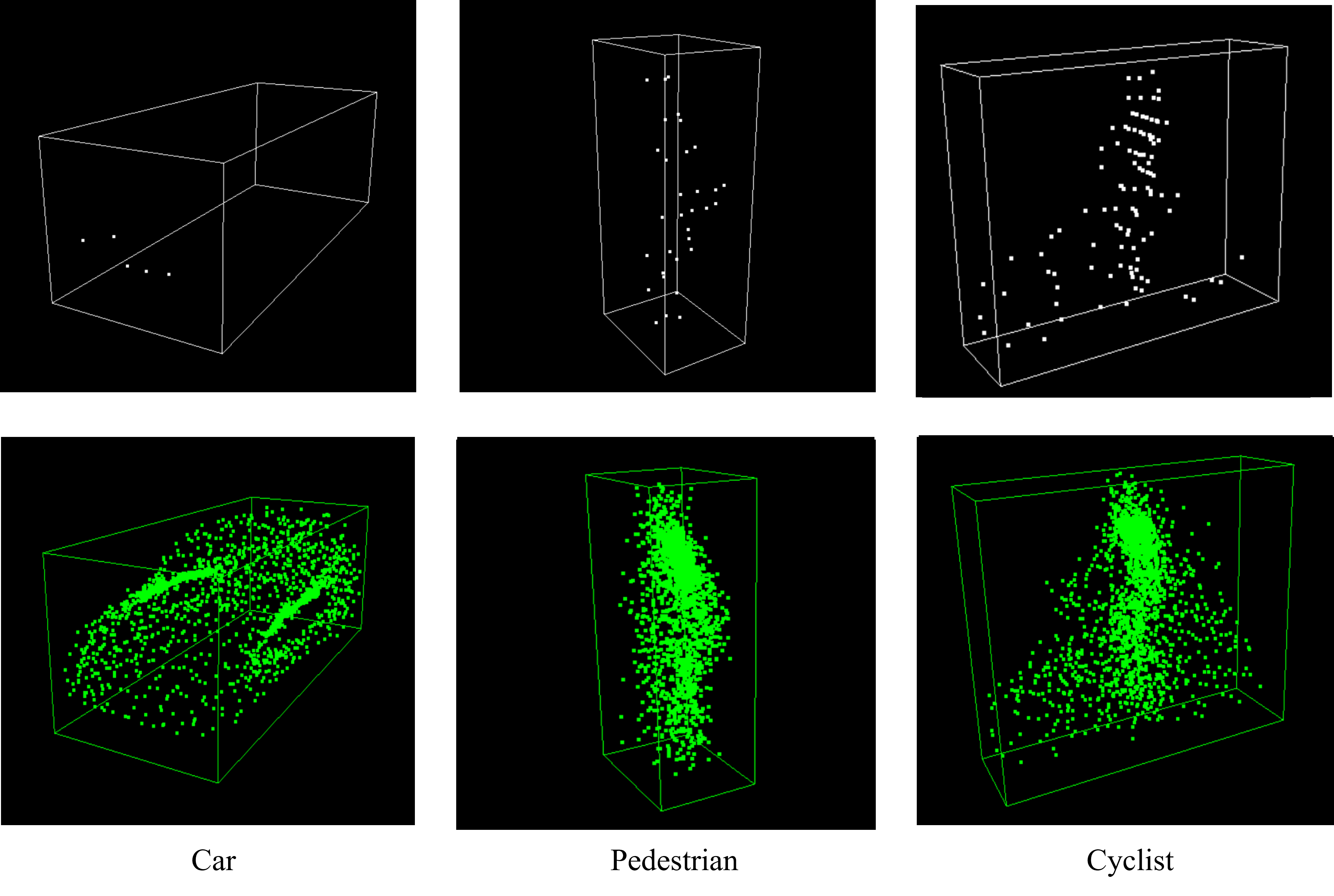
Figure 5: Dense point cloud database for KITTI train dataset. Utilizing a PCN is more effective than manually combining additional points for sparse objects, as rule-based methods struggle to define clear guidelines for aggregating points.

Loss Function. Concretely, we minimize the following loss function $\mathcal{L}_{\text{total}}$:

$$\mathcal{L}_{\text{total}}=\mathcal{L}_{\text{RPN}}+\mathcal{L}_{\text{RCNN}}+\mathcal{L}_{\text{RPG}}$$ (6)

where $\mathcal{L}_{\text{RPN}}$ is the RPN loss, $\mathcal{L}_{\text{RCNN}}$ is the proposal refinement loss, and $\mathcal{L}_{\text{RPG}}$ is the point generation loss. $\mathcal{L}_{\text{RPN}}$ and $\mathcal{L}_{\text{RCNN}}$ are fundamentally similar, predicting RoIs’ classes and bounding boxes. For bounding box regression, only positive predictions that exceed the intersection-over-union (IoU) threshold participate in loss calculation using the smooth-L1 loss. For class classification, focal loss [31] is used for the RPN, and binary cross-entropy is used for the detection head.

III-E Dense Dataset Construction

Most LiDAR datasets, do not have complete object shapes. Therefore, synthesized point clouds from sources such as ShapeNet [32] are often utilized for point cloud completion in methods like [2] and [3]. [33] offers a complete point cloud dataset for KITTI [7] dataset by manually combining the point sets of the best-matching objects within the dataset, without relying on external sources. However, some objects remain incomplete due to point cloud sparsity that cannot be matched. Instead of making dense and complete dataset manually or rule-based method, we employed a point cloud completion network (PCN) [26] that leverages both LiDAR points and image features to reconstruct a more complete dataset from [33]. For the Waymo [8] dataset, we aggregate points from the same objects across several sequences, as it provides object IDs. Additionally, we aggregate flipped points for vehicles and cyclists, assuming they are symmetric. These augmented objects, with a sufficiently large number of points, are used as a training dataset to supervise the PCN in generating additional points, thereby building a more comprehensive ground truth (GT) database. Fig. 5 illustrates our output of PCN for KITTI training dataset.

IV Experiments

Datasets. We conducted experiments using the KITTI [7] dataset, which provides 7,481 training and 7,518 test samples for the following three classes: car, pedestrian, and cyclist. Following the conventions [7], the training samples were split into 3,712 training and 3,769 validation samples. Additionally, we utilized the Waymo Open Dataset (WOD) [8], a large-scale autonomous driving dataset consisting of 798 training and 202 validation sequences for the three classes (i.e., vehicle, pedestrian, and cyclist), captured by five surrounding-view cameras.

Implementation Details. For the KITTI dataset [7], the detection range is set to [0m, 70.4m] along the X-axis, [-40m, 40m] along the Y-axis, and [-3m, 1m] along the Z-axis, as it provides annotations only for objects visible in the camera images. The voxel size is set to (0.05m, 0.05m, 0.1m). We follow common data augmentation strategies, including random flipping along the X-axis, global scaling with a factor in the range [0.95, 1.05], and global rotations about the Z-axis within the range $[-\frac{1}{4\pi},\frac{1}{4\pi}]$. We also adopt ground truth (GT) sampling [13, 34] for multi-modal data, cropping and pasting image bounding boxes corresponding to the sampled objects, where image retains original size. We build our codebase on OpenPCDet [35] and train our method using the Adam optimizer [36] with a one-cycle policy. We trained for 80 epochs with an initial learning rate of 0.01. We used 4 NVIDIA RTX 3090 GPUs for a batch size of 16, and the training time was less than 6 hours.

For the Waymo dataset [8], the detection range is set to [-75.2m, 75.2m] along both the X-axis and Y-axis, and [-2m, 4m] along the Z-axis. The voxel size is set to (0.1m, 0.1m, 0.15m). We employed the same global rotation and scaling augmentation strategies as described for the KITTI dataset, but GT sampling was not used in this case. Other settings are consistent with the KITTI training details, with the number of epochs set to 30 for conventional cases. Due to GPU resource limitations, we used 4% of the training dataset and 20% of the validation dataset, and images are downsampled by 4x. Training was conducted on 4 NVIDIA RTX A6000 GPUs, with a total training time of less than 6 hours.

Evaluation Details. For KITTI [7] dataset, we evaluated our method using mean average precision (mAP) for 40 recall positions (R40), with IoU thresholds set to 0.7, 0.5, and 0.5 for cars, pedestrians, and cyclists, respectively. For Waymo [8] dataset, mAPH (mean average precision by heading) is also used and our evaluation was conducted for all difficulty level: i.e., Level 1 (L1) and 2 (L2), where L1 refers to ground truth boxes with more than 5 points, and L2 refers to boxes with fewer or equal to 5 points.

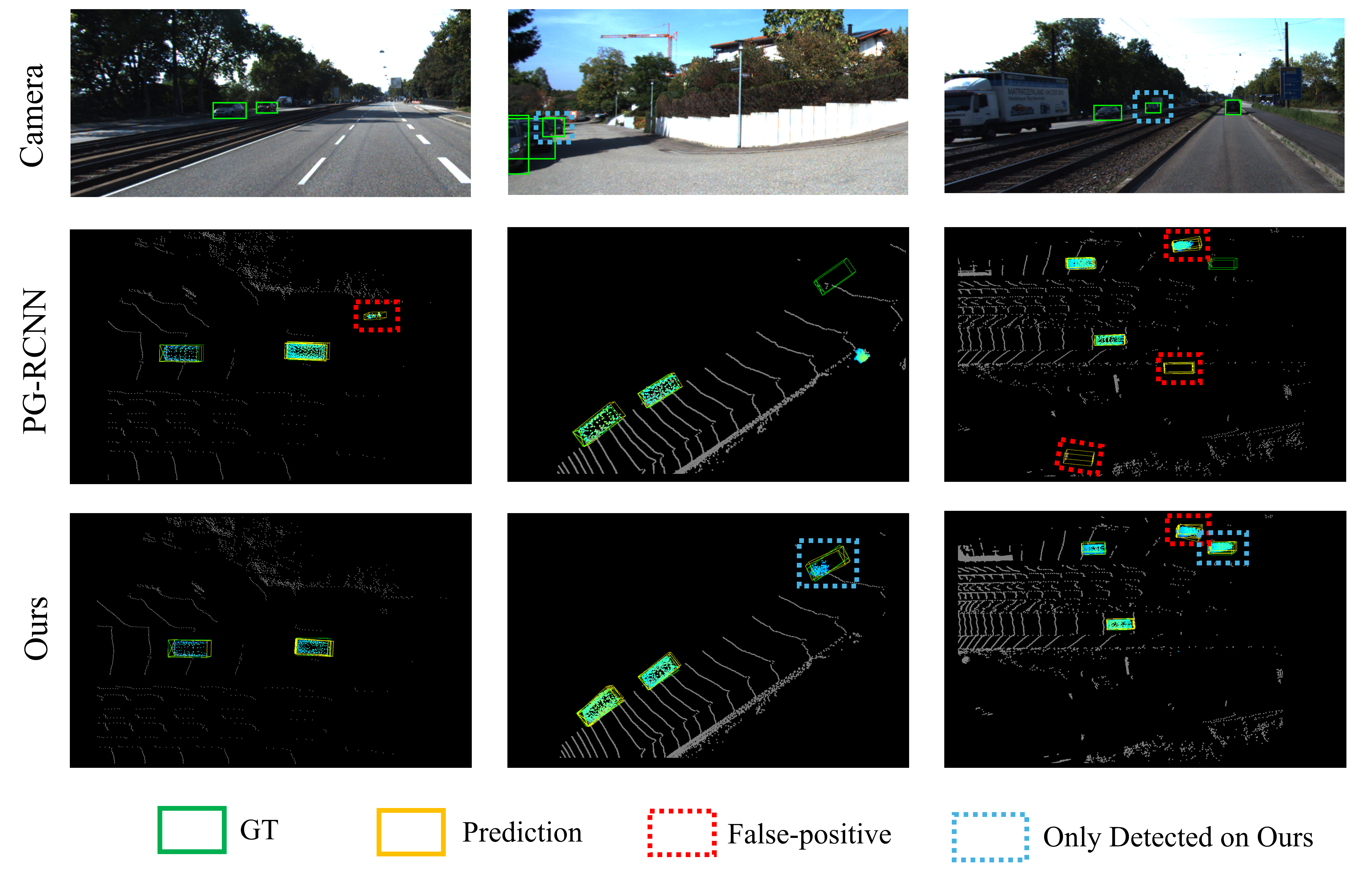
Figure 6: Qualitative comparison between PG-RCNN [4] and our proposed method. Our method demonstrates superior performance in terms of reducing false positives and improving detection of sparse objects, while PG-RCNN [4] struggles in these scenarios.

IV-A Benchmark Results.

Our method is based on PG-RCNN [4], and we reproduced the results from the original code implementation (marked by *). Tables I and II present the performance on the KITTI validation and testing sets, demonstrating significant improvements with our method. This indicates that our approach effectively enhances sparse points, making them denser and easier to capture. Table III illustrates that generating points with image features can have a significant impact when the dataset size is limited, showing the potential for generalizability in data-scarce environments. Additionally, we conducted experiments to evaluate how effectively our method generates and captures objects as the detection range increases. Tables IV and V demonstrate that our method benefits from utilizing image features, particularly at longer ranges.

TABLE IV: mAP by ranges for Cars on KITTI val set.

Method	Car 3DR40			Car BEVR40
	[0, 20)	[20, 40)	[40, inf)	[0, 20)	[20, 40)	[40, inf)
Voxel R-CNN [5]	95.99	82.86	25.71	96.64	90.17	38.52
Baseline* [4]	95.00	83.00	24.34	96.33	90.32	38.42
Ours	96.14	84.24	28.42	97.41	90.95	41.05

TABLE V: mAP for Pedestrians by ranges on Waymo 20% val set.

	Method	Pedestrian 3DR40
		Overall	[0, 30)	[30, 50)	[50, inf)
L1	SECOND* [13]	45.54	52.28	44.55	30.68
	PointPillars* [1]	48.69	57.41	46.09	31.69
	Baseline* [4]	56.06	61.78	56.90	41.73
	Ours	63.59	71.34	62.54	45.26
L2	SECOND* [13]	39.95	49.06	39.80	23.09
	PointPillars* [1]	42.69	53.85	41.15	23.87
	Baseline* [4]	49.30	58.09	51.02	31.48
	Ours	56.23	67.37	56.33	34.44

TABLE VI: Ablation study results on KITTI val set.

Model	SPEPre	CMFF	SPEPost	OverallR40
				Easy	Mod.	Hard
Baseline* [4]	-	-	-	83.21	71.95	67.77
A	$\checkmark$		$\checkmark$	81.27	71.64	68.28
B	$\checkmark$	$\checkmark$		83.81	72.30	68.59
C		$\checkmark$	$\checkmark$	84.06	73.16	69.57
D (ours)	$\checkmark$	$\checkmark$	$\checkmark$	84.61	72.84	69.67

IV-B Qualitative Results.

Fig. 6 illustrates the qualitative results on KITTI validation set comparing the baseline [4] with our method. The baseline suffers from false-positive detections due to the lack of dense semantic priors. In contrast, our method incorporates image features, which helps reduce the number of false positives. Additionally, the baseline [4] struggles to detect distant, sparse objects, whereas our model effectively handles long-range detection and captures sparse objects. Only generated points with confidence scores greater than 0.1 are visualized.

IV-C Ablation Studies.

Effect of Each Component. As shown in Table VI, we evaluated the performance of each module: SPE${}_{\text{Pre}}$, CMFF, and SPE${}_{\text{Post}}$. The results show that utilizing all three modules improves performance across Easy, Moderate, and Hard difficulty levels.

(A) Excluding CMFF and using only SPE${}_{\text{Pre}}$ and SPE${}_{\text{Post}}$ results in lower performance, particularly for Moderate and Hard categories, indicating that cross-modal feature fusion is critical for combining image and point cloud data. (B) Adding CMFF boosts performance, especially in the Moderate category, by enriching point generation with image features. (C) The full configuration further improves results, with SPE${}_{\text{Post}}$ refining points generated by CMFF, particularly benefiting Easy and Hard categories. (D) Our proposed method achieves the highest performance across all categories, especially in the Hard category, confirming the effectiveness of combining SPE${}_{\text{Pre}}$, CMFF, and SPE${}_{\text{Post}}$ for semantic enrichment and spatial refinement.

V Conclusions

In this paper, we introduced the LiDAR-Camera Augmentation Network (LCANet), a novel approach to enhance 3D object detection by generating points through the integration of 2D image features with 3D point clouds. Our method, which includes SPE modules and the CMFF network, addresses the limitations of sparse and incomplete point clouds—common challenges in LiDAR-based detection—by utilizing image features to generate semantically enriched points. To train our method, we employed a point cloud completion network to construct a complete point cloud dataset, which is used to supervise the generation of dense point clouds for the KITTI and Waymo datasets. Through extensive experiments on these datasets, we demonstrated that our method outperforms existing point generation models, particularly in detecting distant and sparse objects, effectively compensating for LiDAR’s limitations in detecting distant objects. We believe that our proposed point generation method will play a crucial role in overcoming the inherent limitations of LiDAR sensors. Future work will focus on further enhancing the generalization capabilities of our method across diverse environments and exploring its potential for real-time applications.

References

- [1] Alex H. Lang, Sourabh Vora, Holger Caesar, Lubing Zhou, Jiong Yang, and Oscar Beijbom. Pointpillars: Fast encoders for object detection from point clouds, 2019.
- [2] Ziyu Li, Yuncong Yao, Zhibin Quan, Wankou Yang, and Jin Xie. Sienet: Spatial information enhancement network for 3d object detection from point cloud, 2021.
- [3] Yanan Zhang, Di Huang, and Yunhong Wang. Pc-rgnn: Point cloud completion and graph neural network for 3d object detection, 2020.
- [4] Inyong Koo, Inyoung Lee, Se-Ho Kim, Hee-Seon Kim, Woo jin Jeon, and Changick Kim. Pg-rcnn: Semantic surface point generation for 3d object detection, 2023.
- [5] Jiajun Deng, Shaoshuai Shi, Peiwei Li, Wengang Zhou, Yanyong Zhang, and Houqiang Li. Voxel r-cnn: Towards high performance voxel-based 3d object detection, 2021.
- [6] Kaiming He, Georgia Gkioxari, Piotr Dollár, and Ross Girshick. Mask r-cnn, 2018.
- [7] Andreas Geiger, Philip Lenz, and Raquel Urtasun. Are we ready for autonomous driving? the kitti vision benchmark suite. In 2012 IEEE conference on computer vision and pattern recognition, pages 3354–3361. IEEE, 2012.
- [8] Pei Sun, Henrik Kretzschmar, Xavier Dotiwalla, Christophe Chouard, Vivek Patnaik, Paul Tsui, Jiquan Guo, Yin Zhou, Yuning Chai, Benjamin Caine, et al. Scalability in perception for autonomous driving: Waymo open dataset. In Proceedings of the IEEE/CVF conference on computer vision and pattern recognition, pages 2446–2454, 2020.
- [9] Charles R. Qi, Hao Su, Kaichun Mo, and Leonidas J. Guibas. Pointnet: Deep learning on point sets for 3d classification and segmentation, 2017.
- [10] Charles R. Qi, Li Yi, Hao Su, and Leonidas J. Guibas. Pointnet++: Deep hierarchical feature learning on point sets in a metric space, 2017.
- [11] Shaoshuai Shi, Xiaogang Wang, and Hongsheng Li. Pointrcnn: 3d object proposal generation and detection from point cloud, 2019.
- [12] Yin Zhou and Oncel Tuzel. Voxelnet: End-to-end learning for point cloud based 3d object detection, 2017.
- [13] Yan Yan, Yuxing Mao, and Bo Li. Second: Sparsely embedded convolutional detection. Sensors, 18(10), 2018.
- [14] Shaoshuai Shi, Chaoxu Guo, Li Jiang, Zhe Wang, Jianping Shi, Xiaogang Wang, and Hongsheng Li. Pv-rcnn: Point-voxel feature set abstraction for 3d object detection, 2021.
- [15] Peng Wu, Lipeng Gu, Xuefeng Yan, Haoran Xie, Fu Lee Wang, Gary Cheng, and Mingqiang Wei. Pv-rcnn++: Semantical point-voxel feature interaction for 3d object detection, 2022.
- [16] Vishwanath A Sindagi, Yin Zhou, and Oncel Tuzel. Mvx-net: Multimodal voxelnet for 3d object detection. In 2019 International Conference on Robotics and Automation (ICRA), pages 7276–7282. IEEE, 2019.
- [17] Sourabh Vora, Alex H. Lang, Bassam Helou, and Oscar Beijbom. Pointpainting: Sequential fusion for 3d object detection, 2020.
- [18] Danfei Xu, Dragomir Anguelov, and Ashesh Jain. Pointfusion: Deep sensor fusion for 3d bounding box estimation, 2018.
- [19] Qi Cai, Yingwei Pan, Ting Yao, Chong-Wah Ngo, and Tao Mei. Objectfusion: Multi-modal 3d object detection with object-centric fusion. In Proceedings of the IEEE/CVF International Conference on Computer Vision (ICCV), pages 18067–18076, October 2023.
- [20] Zhijian Liu, Haotian Tang, Alexander Amini, Xinyu Yang, Huizi Mao, Daniela Rus, and Song Han. Bevfusion: Multi-task multi-sensor fusion with unified bird’s-eye view representation, 2022.
- [21] Junbo Yin, Jianbing Shen, Runnan Chen, Wei Li, Ruigang Yang, Pascal Frossard, and Wenguan Wang. Is-fusion: Instance-scene collaborative fusion for multimodal 3d object detection, 2024.
- [22] Haotian Hu, Fanyi Wang, Jingwen Su, Yaonong Wang, Laifeng Hu, Weiye Fang, Jingwei Xu, and Zhiwang Zhang. Ea-lss: Edge-aware lift-splat-shot framework for 3d bev object detection, 2023.
- [23] Jiachen Sun, Haizhong Zheng, Qingzhao Zhang, Atul Prakash, Z. Morley Mao, and Chaowei Xiao. Calico: Self-supervised camera-lidar contrastive pre-training for bev perception, 2023.
- [24] Xuyang Bai, Zeyu Hu, Xinge Zhu, Qingqiu Huang, Yilun Chen, Hongbo Fu, and Chiew-Lan Tai. Transfusion: Robust lidar-camera fusion for 3d object detection with transformers, 2022.
- [25] Jonah Philion and Sanja Fidler. Lift, splat, shoot: Encoding images from arbitrary camera rigs by implicitly unprojecting to 3d, 2020.
- [26] Wentao Yuan, Tejas Khot, David Held, Christoph Mertz, and Martial Hebert. Pcn: Point completion network. In 3D Vision (3DV), 2018 International Conference on, 2018.
- [27] Yue Wang, Yongbin Sun, Ziwei Liu, Sanjay E. Sarma, Michael M. Bronstein, and Justin M. Solomon. Dynamic graph cnn for learning on point clouds, 2019.
- [28] Ze Liu, Yutong Lin, Yue Cao, Han Hu, Yixuan Wei, Zheng Zhang, Stephen Lin, and Baining Guo. Swin transformer: Hierarchical vision transformer using shifted windows, 2021.
- [29] Tsung-Yi Lin, Piotr Dollár, Ross Girshick, Kaiming He, Bharath Hariharan, and Serge Belongie. Feature pyramid networks for object detection, 2017.
- [30] Ashish Vaswani, Noam Shazeer, Niki Parmar, Jakob Uszkoreit, Llion Jones, Aidan N. Gomez, Lukasz Kaiser, and Illia Polosukhin. Attention is all you need, 2023.
- [31] Tsung-Yi Lin, Priya Goyal, Ross Girshick, Kaiming He, and Piotr Dollar. Focal loss for dense object detection. In Proceedings of the IEEE international conference on computer vision, pages 2980–2988, 2017.
- [32] Angel X. Chang, Thomas Funkhouser, Leonidas Guibas, Pat Hanrahan, Qixing Huang, Zimo Li, Silvio Savarese, Manolis Savva, Shuran Song, Hao Su, Jianxiong Xiao, Li Yi, and Fisher Yu. Shapenet: An information-rich 3d model repository, 2015.
- [33] Qiangeng Xu, Yiqi Zhong, and Ulrich Neumann. Behind the curtain: Learning occluded shapes for 3d object detection, 2021.
- [34] Yanwei Li, Xiaojuan Qi, Yukang Chen, Liwei Wang, Zeming Li, Jian Sun, and Jiaya Jia. Voxel field fusion for 3d object detection, 2022.
- [35] OpenPCDet Development Team. Openpcdet: An open-source toolbox for 3d object detection from point clouds. https://github.com/open-mmlab/OpenPCDet, 2020.
- [36] Diederik P. Kingma and Jimmy Ba. Adam: A method for stochastic optimization, 2017.