(De)-regularized Maximum Mean Discrepancy Gradient Flow

Abstract

We introduce a (de)-regularization of the Maximum Mean Discrepancy (DrMMD) and its Wasserstein gradient flow. Existing gradient flows that transport samples from source distribution to target distribution with only target samples, either lack tractable numerical implementation ($f$-divergence flows) or require strong assumptions, and modifications such as noise injection, to ensure convergence (Maximum Mean Discrepancy flows). In contrast, DrMMD flow can simultaneously (i) guarantee near-global convergence for a broad class of targets in both continuous and discrete time, and (ii) be implemented in closed form using only samples. The former is achieved by leveraging the connection between the DrMMD and the $\chi^{2}$-divergence, while the latter comes by treating DrMMD as MMD with a de-regularized kernel. Our numerical scheme uses an adaptive de-regularization schedule throughout the flow to optimally trade off between discretization errors and deviations from the $\chi^{2}$ regime. The potential application of the DrMMD flow is demonstrated across several numerical experiments, including a large-scale setting of training student/teacher networks.

1 Introduction

Many applications in computational statistics and machine learning involve approximating a probability distribution $\pi$ on $\mathbb{R}^{d}$ (in terms of samples) when only partial information on $\pi$ is accessible. For example, in Bayesian inference, $\pi$ is known up to an intractable normalizing constant for complex models. The setting of interest in this work is the so-called generative modeling setting (Brock et al., 2019; Ho et al., 2020; Song et al., 2020; Franceschi et al., 2024) where one assumes access to a set of samples from the target distribution $\pi$, with the goal being to generate new samples from $\pi$. Recently, a popular framework to perform this task involves solving a minimization problem in $\mathcal{P}(\mathbb{R}^{d})$, the space of probability distributions over $\mathbb{R}^{d}$, by choosing the objective function to be a dissimilarity function $\mathcal{D}(\cdot\|\pi)$ (a distance or divergence) between probability distributions that satisfies: $\mathcal{D}(\nu\|\pi)=0$ if and only if $\nu=\pi$. Since only samples from $\pi$ are available, this problem is solved approximately—yet, the approximate minimizers may converge to $\pi$ as the number of available samples increases. In particular, in the space of probability distributions with bounded second moment $\mathcal{P}_{2}(\mathbb{R}^{d})$, a common approach is to solve this optimization problem by running a (sample-based) approximation of the Wasserstein gradient flow of the functional $\mathcal{F}=\mathcal{D}(\cdot\|\pi)$, which defines a path of distributions with steepest descent for $\mathcal{F}$ with respect to the Wasserstein-2 distance.

In generative modeling, the choice of $\mathcal{D}(\cdot\|\pi)$ depends on two crucial aspects: First, its flow should admit consistent and preferably tractable numerical implementations using only samples from $\pi$, and second, under reasonable assumptions, it should guarantee convergence of its flow to $\pi$, the unique global minimizer. Combined, these two properties ensure that in the large sample limit, this algorithm will generate new samples from the target. Unfortunately, verifying these two properties simultaneously has proved to be a surprisingly challenging task. For instance, recent approaches based on Maximum Mean Discrepancy (MMD) (Arbel et al., 2019; Hertrich et al., 2023b), the sliced-Wasserstein distance (Liutkus et al., 2019) and the Sinkhorn divergence (Genevay et al., 2018) typically admit consistent finite-sample implementations, but their global convergence guarantees—when they exist—do not apply to most practical targets $\pi$ of interest. To guarantee global convergence, one could instead choose $\mathcal{D}$ as an $f$-divergence. For instance, the (reverse) KL divergence and $\chi^{2}$-divergence are geodesically convex (Villani et al., 2009, Definition 16.5) when the target is log-concave (i.e. $\pi\propto e^{-V}$ with $V$ convex) (Ohta and Takatsu, 2011), and hence their flows enjoy better convergence behaviour. However, while the population Wasserstein gradient flows of the $\chi^{2}$ and KL divergences are well-defined (Jordan et al., 1998; Chewi et al., 2020), they do not come naturally with consistent and tractable sample-based implementations. Multiple approaches propose to solve a surrogate optimization problem with samples at each iteration of the flow (Gao et al., 2019; Ansari et al., 2021; Simons et al., 2022; Birrell et al., 2022; Gu et al., 2022; Liu et al., 2023); however it remains to be formally established whether these surrogate problems preserve the desirable convergence guarantees of $f$-divergence flows.

In face of the trade-offs present in the current approaches, a natural question arises: Does there exist a divergence functional $\mathcal{D}(\cdot\|\pi)$ whose gradient flow both globally converges, and admits a tractable consistent sample-based implementation? In this work, we take a step towards a positive answer by constructing a “de-regularized” variant of the Maximum Mean Discrepancy ($\operatorname{DrMMD}$) and its associated Wasserstein gradient flow. We prove that the $\operatorname{DrMMD}$ gradient flow converges exponentially to the global minimum up to a controllable barrier term for targets $\pi$ that satisfy a Poincaré inequality, in both continuous and discrete time regimes. To do so, we establish and leverage a connection between the $\operatorname{DrMMD}$ and the $\chi^{2}$ divergence, an $f$-divergence whose gradient flow benefits from strong convergence guarantees. By alternatively viewing $\operatorname{DrMMD}$ as MMD with a regularized kernel, $\operatorname{DrMMD}$ flow comes with a consistent and tractable implementation when only samples from the target $\pi$ are available. In addition, given the empirical success of using adaptive kernels in MMD-based generative models (Galashov et al., 2024; Li et al., 2017; Arbel et al., 2018), our paper shows theoretically that using adaptive kernels through adaptive regularization indeed improves the convergence of MMD gradient flow.

This paper is organized as follows. Section 2 introduces the necessary background on reproducing kernel Hilbert spaces (RKHS), the $\operatorname{MMD}$, $\chi^{2}$-divergence and Wasserstein gradient flows. Section 3 introduces $\operatorname{DrMMD}$ and shows that $\operatorname{DrMMD}$ is a valid probability divergence that metrizes weak convergence. Section 4 uses $\operatorname{DrMMD}$ as the optimization objective to define a Wasserstein gradient flow in $\mathcal{P}_{2}(\mathbb{R}^{d})$, and analyzes the convergence of $\operatorname{DrMMD}$ flow in continuous time. Sections 5 and 6 defines an implementable $\operatorname{DrMMD}$ particle descent scheme with both time and space discretization and analyzes its convergence. Section 7 discusses other Wasserstein gradient flows related to our $\operatorname{DrMMD}$ flow. Section 8 shows experiments that confirm our theoretical results. The proofs of all results are provided in Section 10 with the technical results being relegated to an appendix.

2 Background

In this section, we present the definitions and notation used throughout the paper.

2.1 Notations

Let $\mathcal{L}^{d}$ be the Lebesgue measure on $\mathbb{R}^{d}$. $\mathcal{P}_{2}(\mathbb{R}^{d})$ denotes the set of all Borel probability measures $\mu$ on $\mathbb{R}^{d}$ with finite second moment. For $\mu\in\mathcal{P}_{2}(\mathbb{R}^{d})$, $\mu\ll\pi$ denotes that $\mu$ is absolutely continuous with respect to $\pi$. We use $\frac{\mathrm{d}\mu}{\mathrm{d}\pi}$ to denote the Radon-Nikodym derivative. We recall the standard definition of the Kullback-Leibler divergence, $\operatorname{KL}(\mu\|\pi)=\int\log(\frac{\mathrm{d}\mu}{\mathrm{d}\pi})\mathrm{d}\mu$ if $\mu\ll\pi$, $+\infty$ else.

For a continuous mapping $T:\mathbb{R}^{d}\to\mathbb{R}^{d}$, $T_{\#}\mu$ denotes the push-forward measure of $\mu$ by $T$. For any $\pi\in\mathcal{P}_{2}(\mathbb{R}^{d})$, $L^{2}(\pi)$ is the Hilbert space of (equivalence class of) functions $f:\mathbb{R}^{d}\to\mathbb{R}$ such that $\int|f|^{2}d\pi<\infty$. We denote by $\|\cdot\|_{L^{2}(\pi)}$ and $\langle\cdot,\cdot\rangle_{L^{2}(\pi)}$ the norm and the inner product of $L^{2}(\pi)$. We denote by $C_{c}^{\infty}(\mathbb{R}^{d})$ the space of infinitely differentiable functions from $\mathbb{R}^{d}$ to $\mathbb{R}$ with compact support. For a vector valued functions $g:\mathbb{R}^{d}\to\mathbb{R}^{p}$, we abuse the notation of $L^{2}(\pi)$ and claim $g\in L^{2}(\pi)$ if $g_{i}\in L^{2}(\pi)$ for all $i=1,\ldots,p$ along with $\|g\|^{2}_{L^{2}(\pi)}:=\sum_{i=1}^{p}\|g_{i}\|^{2}_{L^{2}(\pi)}$.

If $f:\mathbb{R}^{d}\to\mathbb{R}$ is differentiable, we denote by $\nabla f$ the gradient of $f$ and $\mathbf{H}f$ its Hessian. $f$ is $\alpha$-strongly convex if $\mathbf{H}f\succeq\alpha\mathrm{I}$, i.e, $\mathbf{H}f(x)-\alpha\mathrm{I}$ is positive semi-definite for any $x$, where $\mathrm{I}$ is the identity matrix (also denotes an identity operator depending on the context). For a vector valued function $g:\mathbb{R}^{d}\to\mathbb{R}^{d}$, if $g_{i}$ is differentiable for all $i=1,\cdots,d$, $\nabla\cdot g$ denotes the divergence of $g$. We also denote by $\Delta g$ the Laplacian of $g$, where $\Delta g=\nabla\cdot\nabla g$. We use $\|\cdot\|_{F}$ to denote matrix Frobenius norm. $a\wedge b$ and $a\vee b$ denote the minimum and maximum of $a$ and $b$, respectively.

2.2 Reproducing kernel Hilbert spaces

For a positive semi-definite kernel $k:\mathbb{R}^{d}\times\mathbb{R}^{d}\to\mathbb{R}$, its corresponding reproducing kernel Hilbert space (RKHS) $\mathcal{H}$ is a Hilbert space with inner product $\langle\cdot,\cdot\rangle_{\mathcal{H}}$ and norm $\|\cdot\|_{\mathcal{H}}$ (Aronszajn, 1950), such that (i) $k(x,\cdot)\in\mathcal{H}$ for all $x\in\mathbb{R}^{d}$, and (ii) the reproducing property holds, e.g. for all $f\in\mathcal{H}$, $x\in\mathbb{R}^{d}$, $f(x)=\langle f,k(x,\cdot)\rangle_{\mathcal{H}}$. We denote by $\mathcal{H}^{d}$ the Cartesian product RKHS consisting of elements $f=(f_{1},\dots,f_{d})$ with $f_{i}\in\mathcal{H}$ with inner product $\langle f,g\rangle_{\mathcal{H}^{d}}=\sum_{i=1}^{d}\langle f_{i},g_{i}\rangle_{\mathcal{H}}$.

When $\int k(x,x)\mathrm{d}\pi(x)<\infty$, $\mathcal{H}$ can be canonically injected into $L^{2}(\pi)$ using the operator $\iota_{\pi}:\mathcal{H}\to L^{2}(\pi),\,f\mapsto f$ with adjoint $\iota_{\pi}^{\ast}:L^{2}(\pi)\rightarrow\mathcal{H}$ given by

$$\iota_{\pi}^{\ast}f(\cdot)=\int k(x,\cdot)f(x)\mathrm{d}\pi(x).$$

The operator $\iota_{\pi}$ and its adjoint can be composed to form an $L^{2}(\pi)$ endomorphism $\mathcal{T}_{\pi}\coloneqq\iota_{\pi}\iota_{\pi}^{\ast}$ called the integral operator, and a $\mathcal{H}$ endomorphism $\Sigma_{\pi}:=\iota_{\pi}^{\ast}\iota_{\pi}=\int k(\cdot,x)\otimes k(\cdot,x)d\pi(x)$ (where $(a\otimes b)c\coloneqq\langle b,c\rangle_{\mathcal{H}}a$ for $a,b,c\in\mathcal{H}$) called the covariance operator. $\mathcal{T}_{\pi}$ is compact, positive, self-adjoint, and can thus be diagonalized into an orthonormal system in $\left\{e_{i}\right\}_{i\geq 1}$ of $L^{2}(\pi)$ with associated eigenvalues $\varrho_{1}\geq\cdots\varrho_{i}\geq\cdots\geq 0$.

In this paper, we make the following assumption on our kernel.

Assumption 1.

$k:\mathbb{R}^{d}\times\mathbb{R}^{d}\to\mathbb{R}$ is a continuous and $c_{0}$-universal kernel, and there exists $K>0$ such that $\sup_{x}k(x,x)\leq K$.

We refer the reader to Carmeli et al. (2010) for the definition of $c_{0}$-universal kernel. The implication of 1 is that the RKHS $\mathcal{H}$ is compactly embedded into $L^{2}(\pi)$ (Steinwart and Scovel, 2012, Lemma 2.3), and hence $k(x,x^{\prime})$ has a absolute, uniform and pointwise convergent Mercer representation (Steinwart and Scovel, 2012, Corollary 3.5),

$$k(x,x^{\prime})=\sum_{i\geq 1}\varrho_{i}e_{i}(x)e_{i}(x^{\prime}),$$ (1)

for any $x$ and $x^{\prime}$ in the support of $\pi$. Since the kernel is $c_{0}$-universal, the RKHS $\mathcal{H}$ is dense in $L^{2}(\pi)$ for all Borel probability measures $\pi$ (Sriperumbudur et al., 2011, Section 3.1) and $\{e_{i}\}_{i\geq 1}$ becomes an orthornormal basis of $L^{2}(\pi)$ (Steinwart and Scovel, 2012, Theorem 3.1).

The power of the integral operator $\mathcal{T}_{\pi}^{r}$ is defined as $\mathcal{T}_{\pi}^{r}f:=\sum_{i\geq 1}\varrho_{i}^{r}\left\langle f,e_{i}\right\rangle_{L^{2}(\pi)}e_{i},f\in L^{2}(\pi)$. For $f\in\operatorname{Ran}(\mathcal{T}_{\pi}^{r})$, there exists $q\in L^{2}(\pi)$ such that $f=\mathcal{T}_{\pi}^{r}q$. The exponent $r$ quantifies the smoothness of the range space relative to the original RKHS $\mathcal{H}$ with $0<r<\frac{1}{2}$ (resp. $r>\frac{1}{2}$) yields spaces that are less (resp. more) smooth than $\mathcal{H}$ with $\operatorname{Ran}(\mathcal{T}_{\pi}^{1/2})$ being isometrically isomorphic to $\mathcal{H}$ (Cucker and Zhou, 2007; Fischer and Steinwart, 2020).

We make an additional assumption—commonly employed in the kernel-based gradient flow literature (Glaser et al., 2021; He et al., 2024; Korba et al., 2020; Arbel et al., 2019)—on the regularity of the kernel that will be employed in studying the $\operatorname{DrMMD}$ gradient flow.

Assumption 2.

$k:\mathbb{R}^{d}\times\mathbb{R}^{d}\to\mathbb{R}$ is twice differentiable in the sense of (Steinwart and Christmann, 2008, Definition 4.35), i.e., for $i,j\in\{1,\cdots,d\}$, both $\partial_{i}\partial_{i+d}k$ and $\partial_{i}\partial_{j}\partial_{i+d}\partial_{j+d}k$ exist and are continuous. There exist constants $K_{1d},K_{2d}>0$ such that $\left\|\nabla_{1}k(x,\cdot)\right\|_{\mathcal{H}^{d}}:=\sum_{i=1}^{d}\left\|\partial_{i}k(x,\cdot)\right\|_{\mathcal{H}}\leq\sqrt{K_{1d}}$ and $\left\|\mathbf{H}_{1}k(x,\cdot)\right\|_{\mathcal{H}^{d\times d}}:=\sum_{i,j=1}^{d}\left\|\partial_{i}\partial_{j}k(x,\cdot)\right\|_{\mathcal{H}}\leq\sqrt{K_{2d}}$ for all $x\in\mathbb{R}^{d}$.

Many kernels satisfy both 1 and 2, including the class of bounded, continuous, and translation invariant kernel on $\mathbb{R}^{d}$ whose Fourier transforms has finite second and fourth moments. This is easy to verify by employing the Fourier transform representation of the RKHS (Wendland, 2004, Theorem 10.12) and noting that the finiteness of the RKHS norm of $\nabla_{1}k(\cdot,x)$ and $\mathbf{H}_{1}k(\cdot,x)$ for all $x$ corresponds to the existence and finiteness of the second and fourth moments of the Fourier transform of the kernel, respectively. This condition is satisfied by the Gaussian kernel, Matérn kernels of order $\nu$ with $\nu+\frac{d}{2}\geq 2$ and the inverse multiquadratic kernel.

2.3 Maximum mean discrepancy and $\chi^{2}$-divergence

The Maximum Mean Discrepancy ($\operatorname{MMD}$) (Gretton et al., 2012) between $\mu$ and $\pi$ is defined as the RKHS norm of the difference between the mean embeddings $m_{\mu}:=\int k(x,\cdot)d\mu(x)$ and $m_{\pi}:=\int k(x,\cdot)d\pi(x)$.

$$\operatorname{MMD}(\mu\|\pi) \coloneqq\left\|\int k(x,\cdot)d\mu(x)-\int k(x,\cdot)d\pi(x)\right\|_{\mathcal{H}}=\left\|m_{\mu}-m_{\pi}\right\|_{\mathcal{H}}.$$ (2)

The function $m_{\mu}-m_{\pi}$ is often referred to as the “witness function”. When the kernel $k$ is $c_{0}$-universal, $\operatorname{MMD}(\mu\|\pi)=0$ if and only if $\mu=\pi$, and the $\operatorname{MMD}$ metrizes the weak topology between probability measures (Sriperumbudur et al., 2010; Sriperumbudur, 2016). Given samples $(x_{1},\dots,x_{n})$ and $(y_{1},\dots,y_{m})$ from $\mu$ and $\pi$ respectively, the $\operatorname{MMD}$ can be consistently estimated in multiple ways (Gretton et al., 2012). For instance, one can compute its “plug-in” estimator, e.g. $\operatorname{MMD}(\hat{\mu}\|\hat{\pi})$, where $\widehat{\mu}\coloneqq\frac{1}{n}\sum_{i=1}^{n}\delta_{x_{i}}$ and $\widehat{\pi}\coloneqq\frac{1}{n}\sum_{i=1}^{n}\delta_{y_{i}}$.

The $\chi^{2}$-divergence — a member of the family of $f$-divergences (Rényi, 1961) — is defined as the variance of the Radon-Nikodym derivative $\frac{d\mu}{d\pi}$ under $\pi$:

$$\chi^{2}(\mu\|\pi)\coloneqq\int\left(\frac{\mathrm{d}\mu}{d\pi}-1\right)^{2}\mathrm{d}\pi,$$

when $\mu\ll\pi$, and $+\infty$ otherwise. The $\chi^{2}$-divergence has a well-known variational form (Nowozin et al., 2016; Nguyen et al., 2010):

$$\chi^{2}(\mu\|\pi)=\sup_{h\in\mathcal{M}(\mathbb{R}^{d})}\int hd\mu-\int\left(h+\frac{1}{4}h^{2}\right)d\pi,$$

where $\mathcal{M}(\mathbb{R}^{d})$ denote the set of all measurable functions from $\mathbb{R}^{d}$ to $\mathbb{R}$. When $\mu\ll\pi$, we prove in B.1 that the optimal $h^{\ast}=\frac{d\mu}{d\pi}-1\in L^{2}(\pi)$ so that it is sufficient to restrict the variational set to $L^{2}(\pi)$ in contrast to $\mathcal{M}(\mathbb{R}^{d})$ for general $f$-divergences. Since in most cases, $\chi^{2}(\hat{\mu}\|\hat{\pi})=+\infty$, the $\chi^{2}$-divergence does not admit plug-in estimators, and estimating it consistently involves more complicated strategies (Nguyen et al., 2010).

2.4 Wasserstein gradient flows

Gradient flows are dynamics that use local (e.g. differential) information about a given functional in order to minimize it as fast as possible. Their exact definition depends on the nature of the input space; in the familiar case of Euclidean space $\mathbb{R}^{d}$, the gradient flow of a sufficiently regular $F:\mathbb{R}^{d}\to\mathbb{R}$ given some initial condition $x_{0}$ is given by the solution $(x_{t})_{t\geq 0}$ of $\partial_{t}x_{t}=-v(x_{t})$, where $v$ is the Fréchet subdifferential of $F$, a generalization of the notion of derivative to non-smooth functions (Kruger, 2003).

Gradient flows can be extended from Euclidean spaces to the more general class of metric spaces (Ambrosio et al., 2005). When the metric space in question is $\mathcal{P}_{2}(\mathbb{R}^{d})$ endowed with the Wasserstein-$2$ distance, this gradient flow is called the Wasserstein gradient flow $(\mu_{t})_{t\geq 0}$. The Wasserstein gradient flow of $\mathcal{F}:\mathcal{P}_{2}(\mathbb{R}^{d})\to\mathbb{R}$ takes the particular form (Ambrosio et al., 2005, Lemma 10.4.1):

$$\partial_{t}\mu_{t}+\nabla\cdot\left(\mu_{t}v_{t}\right)=0,$$ (3)

where $v_{t}$ is the Fréchet subdifferential of $\mathcal{F}:\mathcal{P}_{2}(\mathbb{R}^{d})\to\mathbb{R}$ evaluated at $\mu_{t}$ (Ambrosio et al., 2005, Definition 11.1.1). (3) is an instance of the continuity equation with velocity field $v_{t}$: under these dynamics, the mass of $\mu_{t}$ is transported in the direction $v_{t}$ that decreases $\mathcal{F}$ at the fastest rate at each time $t$. While (3) can be time-discretized in various ways (Santambrogio, 2017; Ambrosio et al., 2005), in this work, we will focus on the forward Euler scheme, defined as $\mu_{n+1}\coloneqq(\mathrm{I}-\gamma v_{n})_{\#}\mu_{n}$ where $\gamma>0$ is a step size parameter. Such a scheme is also known as the Wasserstein Gradient Descent of $\mathcal{F}$.

Just as gradient descent in Euclidean spaces, an instrumental property to characterize the convergence of the Wasserstein gradient descent of a functional $\mathcal{F}$ is given by its geodesic convexity and smoothness. Among various ways, one can consider to characterize convexity and smoothness through lower and upper bounds on the Wasserstein Hessian of the functional $\mathcal{F}$ (Villani et al., 2009, Proposition 16.2). Given any $\phi\in C_{c}^{\infty}(\mathbb{R}^{d})$ that defines a constant speed geodesic starting at $\mu$: $\rho_{t}=(\mathrm{I}+t\nabla\phi)_{\#}\mu$ for $0\leq t\leq 1$, the Wasserstein Hessian of a functional $\mathcal{F}:\mathcal{P}_{2}(\mathbb{R}^{d})\to\mathbb{R}$ at $\mu$, denoted as $\operatorname{Hess}\mathcal{F}_{\mid\mu}$, is an operator from $L^{2}(\mu)$ to $L^{2}(\mu)$:

$$\langle\operatorname{Hess}\mathcal{F}_{\mid\mu}\nabla\phi,\nabla\phi\rangle_{L^{2}(\mu)}=\frac{d^{2}}{dt^{2}}\Big{|}_{t=0}\mathcal{F}(\rho_{t}).$$

A functional $\mathcal{F}$ is said to be geodesically $M$-smooth at $\mu$ if $\langle\operatorname{Hess}\mathcal{F}_{\mid\mu}\nabla\phi,\nabla\phi\rangle_{L^{2}(\mu)}\leq M\|\nabla\phi\|_{L^{2}(\mu)}$, and is said to be geodesically $\Lambda$-convex at $\mu$ if $\langle\operatorname{Hess}\mathcal{F}_{\mid\mu}\nabla\phi,\nabla\phi\rangle_{L^{2}(\mu)}\geq\Lambda\|\nabla\phi\|_{L^{2}(\mu)}$. Additionally, $\mathcal{F}$ is geodesically semiconvex if $-\infty<\Lambda<0$ and geodesically strongly convex if $\Lambda>0$. Generally, a functional $\mathcal{F}$ that is both smooth and strongly convex is preferred, because its Wasserstein gradient descent has exponential rate of convergence under small enough step size $\gamma$ (Boyd and Vandenberghe, 2004, Section 9.3.1)(Bonet et al., 2024).

$\operatorname{MMD}$ and $\chi^{2}$ flows

Given some probability measure $\pi\in\mathcal{P}_{2}(\mathbb{R}^{d})$, the $\operatorname{MMD}$ flow (resp. $\chi^{2}$ flow) is the Wasserstein gradient flow of the functional $\mathcal{F}_{\operatorname{MMD}}(\cdot)=\operatorname{MMD}(\cdot\|\pi)$ (resp. $\mathcal{F}_{\chi^{2}}(\cdot)=\chi^{2}(\cdot\|\pi)$). As with the $\operatorname{MMD}$, the $\operatorname{MMD}$ flow has an analytic finite sample implementation and may be used to construct generative modelling algorithms  (Hertrich et al., 2023b, 2024). The Wasserstein Hessian of $\mathcal{F}_{\operatorname{MMD}}$ for smooth kernels is not positively lower bounded (Arbel et al., 2019, Proposition 5), however, so $\operatorname{MMD}$ flow only converges up to an unknown barrier (Arbel et al., 2019, Theorem 6), with global convergence only under a strong (and unverifiable) assumption (Arbel et al., 2019, Proposition 7). More recent works  (Boufadène and Vialard, 2024) have demonstrated the global convergence of the $\operatorname{MMD}$ flow when using the Coulomb kernel. This kernel is non-smooth, however, which complicates numerical implementations. In contrast, the Wasserstein Hessian of $\mathcal{F}_{\chi^{2}}$ is positively lower bounded (Ohta and Takatsu, 2011) for log-concave targets $\pi$, so $\mathcal{F}_{\chi^{2}}$ is geodesically strongly convex and $\chi^{2}$ flow enjoys exponential rate of convergence. The exponential convergence of $\chi^{2}$ flow towards the global minimum in fact holds for a broader class of targets $\pi$ that satisfy a Poincaré inequality (Chewi et al., 2020). The $\chi^{2}$ flow has so far lacked a tractable sample-based implementation, however, so it has not been widely used in practice.

In the following sections, we will introduce a new Wasserstein gradient flow which combines the computational advantages of the MMD flow with the convergence properties of the $\chi^{2}$ flow.

3 (De)-regularized Maximum Mean Discrepancy ($\operatorname{DrMMD}$)

In this section, we introduce a (de)-regularized version of maximum mean discrepancy, or $\operatorname{DrMMD}$ in short. The $\operatorname{DrMMD}$ is rooted in a unified representation of the MMD and the $\chi^{2}$-divergence, given in the following proposition, which is proved in Section 10.1.

Proposition 3.1 ($\operatorname{MMD}$ and $\chi^{2}$-divergence).

Suppose $\frac{d\mu}{d\pi}-1\in L^{2}(\pi)$ for $\mu,\pi\in\mathcal{P}_{2}(\mathbb{R}^{d})$. Then

$$\operatorname{MMD}^{2}(\mu\|\pi)=\left\|\mathcal{T}_{\pi}^{1/2}\left(\frac{d\mu}{d\pi}-1\right)\right\|^{2}_{L^{2}(\pi)} \text{ and }\,\,\chi^{2}(\mu\|\pi)=\left\|\mathrm{I}\left(\frac{d\mu}{d\pi}-1\right)\right\|^{2}_{L^{2}(\pi)}.$$

Remark 3.1.

The $\chi^{2}$ identity follows from the definition but is provided for comparison purposes. Together, these identities express both the MMD and the $\chi^{2}$-divergence as functionals of the (centered) density ratio $\frac{d\mu}{d\pi}-1$. While the $\chi^{2}$-divergence directly computes the $L^{2}(\pi)$ norm of the centred ratio, the $\operatorname{MMD}^{2}$ first computes the image by the operator $\mathcal{T}_{\pi}^{1/2}$ before taking the $L^{2}(\pi)$ norm. The smoothing effect of the compact operator $\mathcal{T}_{\pi}^{1/2}$—note that $\mathcal{T}_{\pi}$ is compact if $k$ is bounded as assumed in 1—has both positive and negative consequences: $\mathcal{F}_{\operatorname{MMD}}(\cdot)=\operatorname{MMD}^{2}(\cdot\|\pi)$ admits finite sample estimators but is not geodesically convex, making the first-order optimization of MMD objective (as done in generative modeling) challenging (Arbel et al., 2019). In contrast, $\mathcal{F}_{\chi^{2}}(\cdot)=\chi^{2}(\cdot\|\pi)$ is geodesically convex for log-concave targets $\pi$ (Ohta and Takatsu, 2011) but is hard to estimate with samples.

With these facts in mind, we introduce a divergence whose purpose is to combine the beneficial properties of both the $\chi^{2}$-divergence and $\operatorname{MMD}$. To do so, this divergence computes the $L^{2}(\pi)$ norm of the image of $\frac{d\mu}{d\pi}-1$ by an alternative operator which interpolates between $\mathrm{I}$ and $\mathcal{T}_{\pi}^{1/2}$. We set this operator to be $((\mathcal{T}_{\pi}+\lambda\mathrm{I})^{-1}\mathcal{T}_{\pi})^{1/2}$, where $\lambda>0$ is a regularization parameter. The operator $((\mathcal{T}_{\pi}+\lambda\mathrm{I})^{-1}\mathcal{T}_{\pi})^{1/2}$ can be seen as a (de)-regularization of the operator $\mathcal{T}_{\pi}^{1/2}$ used by the MMD—- a similar idea has been used in kernel Fisher discriminant analysis (Mika et al., 1999), goodness-of-fit testing (Balasubramanian et al., 2021; Hagrass et al., 2023), and two-sample testing (Harchaoui et al., 2007; Hagrass et al., 2024). We call the resulting divergence the (De)-regularized Maximum Mean Discrepancy ($\operatorname{DrMMD}$).

Definition 1 ($\operatorname{DrMMD}$).

Suppose $\frac{d\mu}{d\pi}-1\in L^{2}(\pi)$ where $\mu,\pi\in\mathcal{P}_{2}(\mathbb{R}^{d})$. Then the (de)-regularized maximum mean discrepancy ($\operatorname{DrMMD}$) between $\mu,\pi\in\mathcal{P}_{2}(\mathbb{R}^{d})$ is defined as

$$\operatorname{DrMMD}(\mu||\pi) =(1+\lambda)\left\|\left((\mathcal{T}_{\pi}+\lambda\mathrm{I})^{-1}\mathcal{T}_{\pi}\right)^{1/2}\left(\frac{d\mu}{d\pi}-1\right)\right\|_{L^{2}(\pi)}^{2},$$ (4)

where $\lambda>0$.

While all the three operators, $\mathrm{I}$, $\mathcal{T}_{\pi}$ and $(\mathcal{T}_{\pi}+\lambda\mathrm{I})^{-1}\mathcal{T}_{\pi}$ are diagonalizable in the same eigenbasis of $L^{2}(\pi)$, the key difference between them lies in the behavior of their eigenvalues. The identity operator $\mathrm{I}$ has all eigenvalues $1$, the integral operator $\mathcal{T}_{\pi}$ has eigenvalues $(\varrho_{i})_{i\geq 1}$ which decay to zero as $i\rightarrow\infty$ and the (de)-regularized integral operator $(\mathcal{T}_{\pi}+\lambda\mathrm{I})^{-1}\mathcal{T}_{\pi}$ has eigenvalues $\left(\varrho_{i}/(\varrho_{i}+\lambda)\right)_{i\geq 1}$ which either decay to zero or converge to 1 depending on the choice of $\lambda$ as $i\rightarrow\infty$. $(\mathcal{T}_{\pi}+\lambda\mathrm{I})^{-1}\mathcal{T}_{\pi}$ is known in the statistical estimation literature as Tikhonov regularization; alternative definitions of $\operatorname{DrMMD}$ could be obtained by using other regularizing operators, such as Showalter regularization in Engl et al. (1996). In this paper, we primarily focus on Tikhonov regularization and leave other types of regularization for future work.

One of the stated purposes of the $\operatorname{DrMMD}$ is to retain the computational benefits of the MMD, which are crucial for its use in particle algorithms for generative modeling. To this end, we provide an alternative representation of $\operatorname{DrMMD}$ which does not involve the density ratio $\frac{d\mu}{d\pi}$ directly, but only kernel expectations.

Proposition 3.2 (Density ratio–free and variational formulations).

$\operatorname{DrMMD}$ can be alternately represented as

$$\operatorname{DrMMD}(\mu||\pi) =(1+\lambda)\left\|\left(\Sigma_{\pi}+\lambda\mathrm{I}\right)^{-\frac{1}{2}}\left(m_{\mu}-m_{\pi}\right)\right\|_{\mathcal{H}}^{2}$$ (5)

$$=(1+\lambda)\sup_{h\in\mathcal{H}}\left\{\int h\mathrm{~{}d}\mu-\int\left(\frac{h^{2}}{4}+h\right)\mathrm{d}\pi-\frac{\lambda}{4}\|h\|_{\mathcal{H}}^{2}\right\}$$ (6)

with $h_{\mu,\pi}^{\ast}=2\left(\Sigma_{\pi}+\lambda\mathrm{I}\right)^{-1}(m_{\mu}-m_{\pi})$ being the witness function.

The proof is in Section 10.2. The density ratio-free representation (5) contains three expectations under $\mu$ and $\pi$: the mean embeddings $m_{\mu}$ and $m_{\pi}$, and the covariance operator $\Sigma_{\pi}$. Given samples $\{x_{i}\}_{i=1}^{M}\sim\mu$ and $\{y_{i}\}_{i=1}^{N}\sim\pi$, we can construct a plug-in finite sample estimator in (10.14) by replacing $\mu$ and $\pi$ with their empirical counterparts: $\hat{\mu}=\frac{1}{M}\sum_{i=1}^{M}\delta_{x_{i}}$ and $\hat{\pi}=\frac{1}{N}\sum_{i=1}^{N}\delta_{y_{i}}$.

The density ratio-free representation (5) frames $\operatorname{DrMMD}$ as acting on the difference of $m_{\mu}$ and $m_{\pi}$ similarly to MMD. In fact, up to a multiplicative factor $(1+\lambda)$, $\operatorname{DrMMD}$ is $\operatorname{MMD}$ computed with respect to another kernel $\tilde{k}$ defined as

$$\tilde{k}(x,x^{\prime})=\left\langle\left(\Sigma_{\pi}+\lambda\mathrm{I}\right)^{-\frac{1}{2}}k(x,\cdot),\left(\Sigma_{\pi}+\lambda\mathrm{I}\right)^{-\frac{1}{2}}k(x^{\prime},\cdot)\right\rangle_{\mathcal{H}}.$$ (7)

The derivations are provided in Section 10.3. The kernel $\tilde{k}$ is symmetric and positive semi-definite by construction, and its associated reproducing kernel Hilbert space is $\tilde{\mathcal{H}}$. The density ratio-free representation of $\operatorname{DrMMD}$ in 3.2 is already known in (Balasubramanian et al., 2021; Harchaoui et al., 2007; Hagrass et al., 2024, 2023) in the context of non-parametric hypothesis testing.

3.1 Properties of $\operatorname{DrMMD}$

In this section, we establish various properties of $\operatorname{DrMMD}$. As discussed earlier, $\operatorname{DrMMD}$ is constructed to interpolate between $\chi^{2}$-divergence and MMD to exploit the advantages associated with each. The following result formalizes the interpolation property.

Proposition 3.3 (Interpolation property).

Let $\mu,\pi\in\mathcal{P}_{2}(\mathbb{R}^{d})$. If 1 holds and $\frac{d\mu}{d\pi}-1\in L^{2}(\pi)$, then

$$\lim_{\lambda\rightarrow 0}\operatorname{DrMMD}(\mu\|\pi)=\chi^{2}(\mu\|\pi),\quad\text{and}\quad\lim_{\lambda\rightarrow\infty}\operatorname{DrMMD}(\mu\|\pi)=\mathrm{MMD}^{2}(\mu\|\pi).$$

3.3, whose proof can be found in Section 10.4, shows that $\operatorname{DrMMD}$ asymptotically becomes a probability divergence in the small and large $\lambda$ regimes. We seek to use $\operatorname{DrMMD}$ as a minimizing objective in generative modeling algorithms, however, so we need to ensure that $\operatorname{DrMMD}$ is a probability divergence for any fixed value of $\lambda$. This result holds, as shown next.

Proposition 3.4 ($\operatorname{DrMMD}$ is a probability divergence).

Under 1, for any $\lambda\in\left(0,\infty\right)$, $\operatorname{DrMMD}$ is a probability divergence, i.e., $\operatorname{DrMMD}(\mu\|\pi)\geq 0$, with equality iff $\mu=\pi$. Moreover, $\operatorname{DrMMD}$ metrizes the weak topology between probability measures, i.e., $\operatorname{DrMMD}(\mu_{n}\|\pi)\to 0$ iff $\mu_{n}$ converges weakly to $\pi\in\mathcal{P}_{2}(\mathbb{R}^{d})$ as $n\rightarrow\infty$.

As MMD with $c_{0}$-universal kernels metrizes the weak convergence of distributions (Sriperumbudur, 2016; Simon-Gabriel et al., 2023), 3.4, whose proof can be found in Section 10.5, shows that for any $\lambda>0$, $\operatorname{DrMMD}$ is “MMD–like” topologically speaking, and is different from the $\chi^{2}$-divergence which induces a strong topology (Agrawal and Horel, 2021).

Remark 3.2.

$\operatorname{DrMMD}$ is a specific case of a so-called “Moreau envelopes of $f$-divergences in reproducing kernel Hilbert spaces” introduced in Neumayer et al. (2024), when the $f$-divergence is taken as the $\chi^{2}$-divergence. This connection is uncovered by the variational formulation of $\operatorname{DrMMD}$ in (6). In contrast to general $f$-divergences, the Moreau envelope of the $\chi^{2}$-divergence enjoys a closed-form expression, as we highlight in this paper with various analytical formulas for $\operatorname{DrMMD}$. The interpolation property (3.3) and the metrization of weak convergence (3.4) are proved concurrently in Corollary 12 and 13 of Neumayer et al. (2024) relying on formulation via Moreau envelopes. In our case, we use direct computations thanks to the closed form of $\operatorname{DrMMD}$.

4 Wasserstein Gradient Flow of $\operatorname{DrMMD}$

Having introduced the $\operatorname{DrMMD}$ in the previous section, we now construct and analyze its Wasserstein Gradient Flow (WGF). As discussed in Section 2, WGFs define dynamics $(\mu_{t})_{t\geq 0}$ in Wasserstein-2 space that minimize a given functional $\mathcal{F}$ by transporting $\mu_{t}$ in the direction of steepest descent, given by the Fréchet subdifferential of $\mathcal{F}$ evaluated at $\mu_{t}$. Given some target distribution $\pi$ from which we wish to sample, the WGF of $\mathcal{F}_{\operatorname{DrMMD}}(\cdot)=\operatorname{DrMMD}(\cdot\|\pi)$, called $\operatorname{DrMMD}$ flow, has the potential to form the basis of a generative modeling algorithm, since $\mu_{t}$ progressively minimizes its distance (in the DrMMD sense) to the target $\pi$.

To fulfill this potential, two additional ingredients are necessary. The first is to formally establish that $\mu_{t}$ reaches the global minimizer $\pi$, and the second is to design a tractable finite-sample algorithm that inherits the convergence properties of the original $\operatorname{DrMMD}$ flow. We defer the second point to Section 5 and focus in this section on showing how $\operatorname{DrMMD}$ benefits from its interpolation towards $\chi^{2}$-divergence such that the $\operatorname{DrMMD}$ flow achieves near-global convergence for a large class of target distributions.

4.1 $\operatorname{DrMMD}$ flow: Definition, existence, and uniqueness

To prove that the $\operatorname{DrMMD}$ flow is well-defined and admits solutions, the key is to show that the $\mathcal{F}_{\operatorname{DrMMD}}$ admits Fréchet subdifferentials, as formalized in the following proposition.

Proposition 4.1 ($\operatorname{DrMMD}$ gradient flow).

Let $\lambda>0$, and $\mu_{0},\pi\in\mathcal{P}_{2}\left(\mathbb{R}^{d}\right)$. Under 1 and 2, the functional $\mathcal{F}_{\operatorname{DrMMD}}$ admits Fréchet subdifferential of the form $(1+\lambda)\nabla h_{\mu_{t},\pi}^{\ast}$, where $h_{\mu_{t},\pi}^{\ast}$ is the witness function defined in 3.2. Consequently, the $\operatorname{DrMMD}$ flow is well-defined and is the solution to the following equation

$$\partial_{t}\mu_{t}-\nabla\cdot\left(\mu_{t}(1+\lambda)\nabla h_{\mu_{t},\pi}^{\ast}\right)=0.$$ (8)

In addition, the $\operatorname{DrMMD}$ flow starting at $\mu_{0}$ is unique because $\mathcal{F}_{\operatorname{DrMMD}}$ is semiconvex, i.e., for any $\phi\in C_{c}^{\infty}(\mathbb{R}^{d})$ and $\mu\in\mathcal{P}_{2}(\mathbb{R}^{d})$,

$$\left|\left\langle\operatorname{Hess}{\mathcal{F}_{\operatorname{DrMMD}}}_{\mid\mu}\nabla\phi,\nabla\phi\right\rangle_{L^{2}(\mu)}\right|\leq 2(1+\lambda)\frac{2\sqrt{KK_{2d}}+K_{1d}}{\lambda}\|\nabla\phi\|_{L^{2}(\mu)}^{2}.$$ (9)

The proof is in Section 10.6. By recalling the discussion of Wasserstein Hessian in Section 2.4, (9) indicates that $\mathcal{F}_{\operatorname{DrMMD}}$ is both geodesically smooth and geodesically semiconvex, which is expected because $\operatorname{DrMMD}$ is equivalent to $\operatorname{MMD}$ with a regularized kernel $\tilde{k}$ defined in (7) and $\mathcal{F}_{\operatorname{MMD}}$ is both geodesically smooth and geodesically semiconvex (Arbel et al., 2019, Proposition 5). 4.1 is proved concurrently in Corollary 14 and 20 of Neumayer et al. (2024) relying on formulation via Moreau envelopes, while our proof uses the closed-form expression for $\operatorname{DrMMD}$.

4.2 Near-global convergence of $\operatorname{DrMMD}$ flow

Having defined the $\operatorname{DrMMD}$ flow, we are now concerned with its convergence to the target $\pi$. Since $\operatorname{DrMMD}$ is constructed to interpolate between the $\operatorname{MMD}$ and the $\chi^{2}$-divergence, $\operatorname{DrMMD}$ flow is expected to recover the convergence properties of the $\chi^{2}$ flow. With this goal in mind, we first study the Wasserstein Hessian of $\operatorname{DrMMD}$ and prove that it becomes asymptotically positive as $\lambda\to 0$ for strongly log-concave targets $\pi$. Next, to obtain a non-asymptotic convergence rate, we take another route and show that the $\operatorname{DrMMD}$ flow converges to $\pi$ exponentially fast in KL divergence up to a barrier term that vanishes in the small $\lambda$ regime, provided that $\pi$ satisfies a Poincaré inequality.

4.2.1 Near-Geodesic Convexity of $\mathcal{F}_{\operatorname{DrMMD}}$

One popular approach to proving that the $\operatorname{DrMMD}$ flow $(\mu_{t})_{t\geq 0}$ converges to the target $\pi$ in terms of $\operatorname{DrMMD}$ is to show that $\mathcal{F}_{\operatorname{DrMMD}}$ is geodesically convex (Ambrosio et al., 2005, Theorem 4.0.4), or, equivalently in our definition in Section 2.4, its Wasserstein Hessian is positive definite. In the next proposition, we show that the Wasserstein Hessian of $\mathcal{F}_{\operatorname{DrMMD}}$ is indeed positive definite for small enough $\lambda$; however, as we will see below (4.2), the form of the result will not allow us to show convergence besides in the limit $\lambda\rightarrow 0$, which leads us to take a different approach in subsequent sections.

Proposition 4.2 (Near-geodesic convexity of $\mathcal{F}_{\operatorname{DrMMD}}$).

Let $\mu,\pi\in\mathcal{P}_{2}(\mathbb{R}^{d})$, $\phi\in C_{c}^{\infty}(\mathbb{R}^{d})$ and $\mu,\pi\ll\mathcal{L}^{d}$. Under 1 and 2, let $\pi$ be $\alpha$ strongly log-concave, i.e., $\pi\propto\exp(-V)$, $\mathbf{H}V\succeq\alpha\mathrm{I}$, and assume additionally that $x\mapsto\mathbf{H}V(x)$ is continuous. Then for all $\mu$ such that $x\mapsto\nabla\log\mu(x)$ is continuous and $\frac{d\mu}{d\pi}-1\in\mathcal{H}$,

$$\left\langle\operatorname{Hess}{\mathcal{F}_{\operatorname{DrMMD}}}_{\mid\mu}\nabla\phi,\nabla\phi\right\rangle_{L^{2}(\mu)}\geq\alpha(1+\lambda)\int\frac{d\mu}{d\pi}(x)\|\nabla\phi(x)\|^{2}d\mu(x)-R(\lambda,\mu,\nabla\phi),$$ (10)

where $\lim_{\lambda\to 0}R(\lambda,\mu,\nabla\phi)=0$.

The proof can be found in Section 10.7. To obtain this result, we relate the Wasserstein Hessian of $\mathcal{F}_{\operatorname{DrMMD}}$ with that of $\mathcal{F}_{\chi^{2}}$. When $\frac{d\mu}{d\pi}-1\in\mathcal{H}$, they coincide asymptotically as $\lambda\to 0$, showing that the interpolation properties of $\operatorname{DrMMD}$ to the $\chi^{2}$-divergence hold at the level of Wasserstein derivatives. Together with the fact that the Wasserstein Hessian of $\mathcal{F}_{\chi^{2}}$ is positive definite for $\alpha$-strongly log-concave $\pi$ (Ohta and Takatsu, 2011), we obtain the lower bound in (10). It is noteworthy that although $\operatorname{DrMMD}$ can be viewed as squared $\operatorname{MMD}$ with a regularized kernel $\tilde{k}$, the near-geodesic convexity in 4.2 is not observed for standard $\operatorname{MMD}$ with a fixed kernel $k$ because the latter does not interpolate towards $\chi^{2}$-divergence.

Remark 4.1 (Geodesic convexity/smoothness trade-off in $\mathcal{F}_{\operatorname{DrMMD}}$).

The geodesic
smoothness and near-convexity of the functional $\mathcal{F}_{\operatorname{DrMMD}}$ are characterized by (9) and (10) respectively via upper and lower bounds on the Wasserstein Hessian of $\mathcal{F}_{\operatorname{DrMMD}}$. However, (9) and (10) impose contradictory conditions on the (de)-regularization parameter $\lambda$: (9) indicates that $\operatorname{DrMMD}$ is smoother if $\lambda$ is larger while (10) indicates that $\operatorname{DrMMD}$ is more convex if $\lambda$ is small enough. Consequently, there is a trade-off between the geodesic convexity and smoothness of $\mathcal{F}_{\operatorname{DrMMD}}$, which will play an important role in Section 5.

Remark 4.2.

4.2 shows that for fixed $\mu$ and $\nabla\phi$, there exists $\lambda$ small enough yet positive such that $\left\langle\operatorname{Hess}{\mathcal{F}_{\operatorname{DrMMD}}}_{\mid\mu}\nabla\phi,\nabla\phi\right\rangle_{L^{2}(\mu)}>0$ at $\mu$. The remainder term $R(\lambda,\mu,\nabla\phi)$ is only controlled in the limit as $\lambda\rightarrow 0$, however, which complicates the use of 4.2 to show global convergence of the $\operatorname{DrMMD}$ flow. In the next section, we employ a different set of techniques that rely on the Poincaré condition on $\pi$, a condition which, as we show, will ensure a sufficient dissipation of KL divergence along the $\operatorname{DrMMD}$ flow to obtain non-asymptotic near-global convergence.

4.2.2 Near-Global Convergence of $\operatorname{DrMMD}$ flow via Poincaré inequality

Even when a functional $\mathcal{F}$ is not geodesically convex, convergence guarantees for its Wasserstein gradient flow $(\mu_{t})_{t\geq 0}$ can still be obtained if the target $\pi$ satisfies certain functional inequalities. Consider the $\chi^{2}$ flow $(\nu_{t})_{t\geq 0}$, for example: if $\pi$ satisfies the Poincaré inequality, then $(\nu_{t})_{t\geq 0}$ converges exponentially fast to $\pi$ in terms of KL divergence (Chewi et al., 2020, Theorem 1), i.e.,

$$\operatorname{KL}(\nu_{T}\|\pi)\leq\exp\left(-\frac{2T}{C_{P}}\right)\operatorname{KL}(\nu_{0}\|\pi).$$ (11)

Recall that $\pi$ satisfies a Poincaré inequality (Pillaud-Vivien et al., 2020, Definition 1) if for all functions $f\colon\mathbb{R}^{d}\to\mathbb{R}$ such that $f,\nabla f\in L^{2}(\pi)$, there exists a constant $C_{P}>0$ such that

$$\int f(x)^{2}d\pi(x)-\left(\int f(x)d\pi(x)\right)^{2}\leq C_{P}\|\nabla f\|^{2}_{L^{2}(\pi)}.$$ (12)

The smallest constant $C_{P}$ for which (12) holds is called the Poincaré constant. The Poincaré inequality is widely used for studying the convergence of Langevin diffusions (Chewi et al., 2024) and $\chi^{2}$ flow (Chewi et al., 2020; Trillos and Sanz-Alonso, 2020). The Poincaré condition is implied by the strong log-concavity of $\pi$, and is weaker than strong log-concavity because it also allows for nonconvex potentials. The set of probability measures satisfying a Poincaré inequality include distributions with sub-gaussian tails or with exponential tails. This set is also closed under bounded perturbations and finite mixtures (see Vempala and Wibisono (2019) and Chewi et al. (2024) for a more detailed discussion).

Given the interpolation property of DrMMD to $\chi^{2}$-divergence,  (11) suggests investigating the convergence of the $\operatorname{DrMMD}$ flow $(\mu_{t})_{t\geq 0}$ in KL divergence under a Poincaré inequality. To this end, we first derive an upper bound on $\operatorname{KL}(\mu_{t}\|\pi)$ along the $\operatorname{DrMMD}$ flow.

Theorem 4.1 (KL control of the $\operatorname{DrMMD}$ flow).

Suppose $k$ satisfies Assumptions 1 and 2, and the target $\pi$ and $\operatorname{DrMMD}$ gradient flow $\left(\mu_{t}\right)_{t\geq 0}$ satisfy the following conditions:

1. $\pi$ satisfies a Poincaré inequality with constant $C_{P}$.

2. $\mu_{t},\pi\ll\mathcal{L}^{d}$.

3. $\frac{d\mu_{t}}{d\pi}-1\in\operatorname{Ran}(\mathcal{T}_{\pi}^{r})$ with $r>0$, i.e., there exists $q_{t}\in L^{2}(\pi)$ such that $\frac{d\mu_{t}}{d\pi}-1=\mathcal{T}_{\pi}^{r}q_{t}$.

4. $\left\|\nabla\left(\log\pi\right)^{\top}\nabla\left(\frac{d\mu_{t}}{d\pi}\right)\right\|_{L^{2}(\pi)}\leq\mathcal{J}_{t}$ and $\left\|\Delta\left(\frac{d\mu_{t}}{d\pi}\right)\right\|_{L^{2}(\pi)}\leq\mathcal{I}_{t}$.

5. For all $i=1,\ldots,d$, $\lim\limits_{x\to\infty}\left(h_{\mu_{t},\pi}^{\ast}(x)-2\frac{d\mu_{t}}{d\pi}(x)\right)\left(\partial_{i}\frac{d\mu_{t}}{d\pi}(x)\right)\pi(x)\to 0$.

Then, for any $T\geq 0$,

$$\operatorname{KL}(\mu_{T}\|\pi) \leq\exp\left(-\frac{2(1+\lambda)}{C_{P}}T\right)\operatorname{KL}(\mu_{0}\|\pi)$$ (13)

$$+4(1+\lambda)\lambda^{r}\int_{0}^{T}\exp\left(-\frac{2(1+\lambda)}{C_{P}}(T-t)\right)\left\|q_{t}\right\|_{L^{2}(\pi)}(\mathcal{J}_{t}+\mathcal{I}_{t})dt.$$ (14)

The proof, which can be found in Section 10.8, leverages the fact that the $\operatorname{DrMMD}$ can approximate not only the $\chi^{2}$-divergence, but also its Wasserstein gradient. The $\operatorname{DrMMD}$’s approximation properties can be combined with functional inequalities to obtain an upper-bound for the continous-time dissipation of KL divergence along the flow, given by:

$$\frac{d}{dt}\operatorname{KL}(\mu_{t}\|\pi)\leq-\frac{2(1+\lambda)}{C_{P}}\operatorname{KL}(\mu_{t}\|\pi)+\underbrace{4(1+\lambda)\lambda^{r}\left\|q_{t}\right\|_{L^{2}(\pi)}\left(\mathcal{J}_{t}+\mathcal{I}_{t}\right)}_{\text{Approximation error}},$$ (15)

from which 4.1 follows upon applying the Growall’s lemma (Gronwall, 1919). The first term is strictly negative, while the second term is an approximation error term arising from $\operatorname{DrMMD}$ not perfectly matching the $\chi^{2}$-divergence for $\lambda>0$. When $\lambda=0$, 4.1 recovers the exponential decay of KL divergence along $\chi^{2}$ flow in (11).

Remark 4.3.

(i) The second condition assumes that $\mu_{t}$ and $\pi$ have densities.
(ii) The third condition that $\frac{d\mu_{t}}{d\pi}-1\in\operatorname{Ran}(\mathcal{T}_{\pi}^{r})$ is a regularity condition on the density ratio so that it can be well approximated by the witness function $h_{\mu_{t},\pi}^{\ast}$. This assumption is known as the range assumption in the literature of kernel ridge regression (Cucker and Zhou, 2007; Fischer and Steinwart, 2020). We posit that this assumption can be relaxed to $\frac{d\mu_{t}}{d\pi}-1\in L^{2}(\pi)$ as in 3.3 if only asymptotic convergence is needed with no explicit rate.
(iii) The fourth condition is another regularity condition on the density ratio along the flow. This condition is automatically satisfied under a stronger range condition ($r=\frac{1}{2}$) in the third condition, i.e., $\frac{d\mu_{t}}{d\pi}-1\in\mathcal{H}$, along with a moment condition on the score function $\nabla\log\pi$. To see this, notice that we can further write (derivations are provided in Section 10.8)

$$\begin{aligned} \left\|\nabla\left(\log\pi\right)^{\top}\nabla\left(\frac{d\mu_{t}}{d\pi}\right)\right\|_{L^{2}(\pi)}&\leq\sqrt{K_{1d}}\|q_{t}\|_{L^{2}(\pi)}\left\|\nabla\log\pi\right\|_{L^{2}(\pi)}\\ \left\|\Delta\left(\frac{d\mu_{t}}{d\pi}\right)\right\|_{L^{2}(\pi)}&\leq\sqrt{K_{2d}}\|q_{t}\|_{L^{2}(\pi)}.\end{aligned}$$ (16)

(iv) The fifth condition is a boundary condition that allows integration by parts equality in the proof. We highlight that many works (e.g., Theorem 1 of He et al. (2024), Theorem 2 of Nitanda et al. (2022), Lemma 6 of Vempala and Wibisono (2019)) on Wasserstein gradient flow apply integration by parts without explicitly stating this condition.

Additionally, if $\|q_{t}\|_{L^{2}(\pi)}\leq Q$, $\mathcal{J}_{t}\leq\mathcal{J},\,\mathcal{I}_{t}\leq\mathcal{I}$ for all $0\leq t\leq T$, then 4.1 will ensure KL convergence of the $\operatorname{DrMMD}$ flow up to a controllable barrier term, e.g. near global convergence.

Corollary 4.1 (Near global convergence of the $\operatorname{DrMMD}$ flow).

In addition to the assumptions of 4.1, if $\left\|q_{t}\right\|_{L^{2}(\pi)}\leq Q$, $\mathcal{J}_{t}\leq\mathcal{J},\mathcal{I}_{t}\leq\mathcal{I}$ for all $0\leq t\leq T$, where $Q,\mathcal{J},$ and $\mathcal{I}$ are universal constants independent of $\lambda$, then for any $T\geq 0$,

$$\operatorname{KL}(\mu_{T}\|\pi)\leq\exp\left(-\frac{2(1+\lambda)}{C_{P}}T\right)\operatorname{KL}(\mu_{0}\|\pi)+2\lambda^{r}C_{P}Q\left(\mathcal{J}+\mathcal{I}\right).$$

The proof of 4.1 follows directly from upper bounding the second term of (13) with universal constants $\mathcal{Q}$, $\mathcal{J}$ and $\mathcal{I}$, and using the closed-form expression of the resulting integral. 4.1 provides a condition under which the $\operatorname{DrMMD}$ flow will exhibit an exponential rate of convergence (linear convergence) in terms of KL divergence up to an extra approximation error term which vanishes as $\lambda\to 0$. If $\left\|q_{t}\right\|_{L^{2}(\pi)}\leq Q,\mathcal{J}_{t}\leq\mathcal{J},\mathcal{I}_{t}\leq\mathcal{I}$ for all $0\leq t\leq T$ as shown in 4.1, the approximation error is of explicit order $\mathcal{O}(\lambda^{r})$. Therefore in the continuous time regime, to have a smaller approximation error, it is beneficial to use a small (de)-regularization parameter $\lambda$, so that $\operatorname{DrMMD}$ flow operates closer to the regime of $\chi^{2}$ flow. However, as we will see in the next section, when it comes to time-discretized $\operatorname{DrMMD}$ flow, i.e., $\operatorname{DrMMD}$ gradient descent, there is a trade-off between the approximation error and the time discretization error such that the selection of $\lambda$ would require more careful analysis to strike a good balance. Finally, a smaller Poincaré constant $C_{P}$ results in both a faster rate of convergence and a smaller barrier.

Previously, Arbel et al. (2019) established (sublinear) global convergence of the $\operatorname{MMD}$ flow in terms of $\operatorname{MMD}$ distance by assuming that a Lojasiewicz inequality (or a variant of it if additionally performing noise injection, see Arbel et al., 2018, Proposition 8) holds along the flow. Our result thus complements that of Arbel et al. (2019) by showing that MMD-type functionals can achieve near-global convergence for targets satisfying a Poincaré inequality regardless of whether such inequqalities hold, by studying their behavior in the $f$-divergence interpolation regime.

Remark 4.4.

Since $\operatorname{DrMMD}$ is asymmetric in its arguments, the reader may wonder why we focus on the gradient flow of $\operatorname{DrMMD}(\cdot||\pi)$ instead of $\operatorname{DrMMD}(\pi||\cdot)$. From the convergence standpoint, 4.1 shows that $\operatorname{DrMMD}(\cdot||\pi)$ converges globally with an exponential rate up to a small barrier when $\pi$ satisfies Poincaré inequality along with an extra regularity condition on the density ratio. This favorable convergence property is no longer true for $\operatorname{DrMMD}(\pi||\cdot)$. Practically speaking, the Wasserstein gradient of $\operatorname{DrMMD}$ requires inverting a kernel integral operator. It is more efficient to do this just once with a kernel integral operator with respect to $\pi$ as in (4), rather than with respect to $\mu_{t}$ which would happen at each time (as done by He et al. 2024).

Computing the $\operatorname{DrMMD}$ flow is intractable since the dynamics are in continuous-time, and in practice we do not have access to $\pi$, but only samples from it. In the next two sections, we build a tractable approximation of the DrMMD flow which provably achieves near-global convergence under similar assumptions as the ones in Section 4. Compared to the $\operatorname{DrMMD}$ flow, this approximation combines a discretization in time (introduced in Section 5) with a particle-based space-discretization (introduced in Section 6). While the space-discretization techniques that we used are well-known in the Wasserstein gradient flow literature, our time-discretized scheme deviates from standard approaches, which are insufficient to guarantee near-global convergence in our case.

5 Time-discretized $\operatorname{DrMMD}$ flow

In this section, we first construct and analyze the forward Euler scheme of (8), a simple time-discretization of the $\operatorname{DrMMD}$ flow which we call $\operatorname{DrMMD}$ Descent. Compared to the $\operatorname{DrMMD}$ flow, the convergence of $\operatorname{DrMMD}$ gradient descent is affected by an additional smoothness-related time-discretization error that blows up as $\lambda$ approaches 0, thus preventing near-global convergence. To address this issue, we propose in Section 5.2 an alternative discrete-time scheme that adapts the value of regularization coefficient $\lambda$ across the descent iterates, which we call Adaptive $\operatorname{DrMMD}$ Descent. We show that this scheme converges in KL divergence up to a barrier term that vanishes as the discretization step size goes to zero.

5.1 $\operatorname{DrMMD}$ Descent

The forward Euler discretization of the $\operatorname{DrMMD}$ flow (or $\operatorname{DrMMD}$ Descent in short) with step size $\gamma>0$ consists of sequence of probabilities $(\mu_{n})_{n\in\mathbb{N}}$ defined by the recursion

$$\mu_{n+1}=\left(\mathrm{I}-\gamma(1+\lambda)\nabla h_{\mu_{n},\pi}^{\ast}\right)_{\#}\mu_{n},\quad\mu_{n=0}=\mu_{0},$$ (17)

where $h_{\mu_{n},\pi}^{\ast}=2\left(\Sigma_{\pi}+\lambda\mathrm{I}\right)^{-1}\left(m_{\mu_{n}}-m_{\pi}\right)$ is the $\operatorname{DrMMD}$ witness function. This scheme was previously considered in Arbel et al. (2019); in particular, Proposition 4 of Arbel et al. (2019) shows that the discrete-time $\operatorname{MMD}$ dissipation rate along the $\operatorname{MMD}$ Descent iterates follows the (continous time) rate of the $\operatorname{MMD}$ flow up to an error term proportional to the step size $\gamma$ and the smoothness parameters of the problem (the Lipschitz constant of the kernel).

Next, we turn to study the convergence of $\operatorname{DrMMD}$ descent. One way is to treat $\operatorname{DrMMD}$ as $\operatorname{MMD}$ with a regularized kernel $\tilde{k}$ and follow Proposition 4 of Arbel et al. (2019), however this does not quantitatively take into account the role of (de)-regularization parameter $\lambda$ that balances the trade-off between geodesic convexity and smoothness of $\mathcal{F}_{\operatorname{DrMMD}}$. Instead, we adopt the same strategy of Section 4 that exploits the interpolation property of $\operatorname{DrMMD}$ towards $\chi^{2}$-divergence: in the following proposition, we study the dissipation of KL divergence along the $\operatorname{DrMMD}$ Descent when the target $\pi$ satisfies a Poincaré inequality, in which the role of (de)-regularization parameter $\lambda$ is highlighted in the approximation and discretization errors.

Proposition 5.1 (Quasi descent lemma in KL divergence).

Suppose $k$ satisfies Assumptions 1 and 2, and suppose the target $\pi$ and $\operatorname{DrMMD}$ gradient descent iterates $\left(\mu_{n}\right)_{n\in\mathbb{N}}$ satisfy the following:

1. $\pi$ satisfies a Poincaré inequality with constant $C_{P}$ and its potential is $\beta$-smooth, i.e., $\pi\propto\exp(-V)$ with $\mathbf{H}V\preceq\beta\mathrm{I}$.

2. $\mu_{n},\pi\ll\mathcal{L}^{d}$.

3. $\frac{d\mu_{n}}{d\pi}-1\in\operatorname{Ran}(\mathcal{T}_{\pi}^{r})$ with $r>0$, i.e., there exists $q_{n}\in L^{2}(\pi)$ such that $\frac{d\mu_{n}}{d\pi}-1=\mathcal{T}_{\pi}^{r}q_{n}$.

4. $\|q_{n}\|_{L^{2}(\pi)}\leq Q$, $\left\|\nabla V^{\top}\nabla\left(\frac{d\mu_{n}}{d\pi}\right)\right\|_{L^{2}(\pi)}\leq\mathcal{J}$, $\left\|\Delta\left(\frac{d\mu_{n}}{d\pi}\right)\right\|_{L^{2}(\pi)}\leq\mathcal{I}$ for all $n=1,\cdots,n_{max}$.

5. For all $i=1,\ldots,d$, $\lim\limits_{x\to\infty}\left(h_{\mu_{n},\pi}^{\ast}(x)-2\frac{d\mu_{n}}{d\pi}(x)\right)\left(\partial_{i}\frac{d\mu_{n}}{d\pi}(x)\right)\pi(x)\to 0$.

6. There exists a constant $1<\zeta<2$ such that for all $n=1,\ldots,n_{\max}$, the step size $\gamma$ satisfies

   $$\gamma\leq\frac{\zeta-1}{2\zeta(1+\lambda)\sqrt{\chi^{2}\left(\mu_{n}\|\pi\right)\frac{K_{2d}}{\lambda}}}.$$ (18)

Then for all $0\leq n\leq n_{\max}$ and $0<\lambda\leq 1$,

$$\begin{aligned} \operatorname{KL}(\mu_{n+1}\|\pi)-\operatorname{KL}(\mu_{n}\|\pi)&\leq-\frac{2}{C_{P}}\chi^{2}(\mu_{n}\|\pi)\gamma\\ &+\underbrace{4\gamma\lambda^{r}Q\left(\mathcal{J}+\mathcal{I}\right)}_{\text{Approximation error}}+\underbrace{8\gamma^{2}(\beta+\zeta^{2})\chi^{2}(\mu_{n}\|\pi)\frac{K_{1d}+K_{2d}}{\lambda}}_{\text{Discretization error}}.\end{aligned}$$ (19)

The proof is provided in Section 10.9. Conditions 1-5 of 5.1 are similar to conditions 1-5 of 4.1, which assumes a functional inequality on the target $\pi$ and regularity on the density ratio $\frac{d\mu_{n}}{d\pi}-1$. In a similar spirit to 4.1, the fourth regularity condition is automatically satisfied under a stronger range assumption on $\frac{d\mu_{n}}{d\pi}-1$. For the sake of brevity, we directly assume uniform upper bounds in the fourth condition rather than writing it out in a separate corollary like 4.1. Compared to the continuous time regime, two extra conditions are necessary. The first one is a smoothness condition on the potential, $\mathbf{H}V\preceq\beta\mathrm{I}$, which is commonly used in the convergence analysis of discrete-time Langevin-based samplers (Dalalyan, 2017; Dalalyan and Karagulyan, 2019; Durmus et al., 2019; Dalalyan et al., 2022; Vempala and Wibisono, 2019). It can be relaxed to $\nabla V$ being Hölder-continuous with exponent $s\in[0,1]$ (Chatterji et al., 2020). The second one, (18), is an upper bound on the step size $\gamma$, aligning with the principle that step size should be small enough for the discrete-time scheme to inherit the properties of its continuous analog. This condition will be more thoroughly discussed in 5.4 when all the conditions on $\gamma$ in 5.1 and 5.2 are presented.

Remark 5.1 (Approximation-Discretization trade-off of $\operatorname{DrMMD}$ Descent).

If we compare the discrete-time KL dissipation of (19) with its continuous-time counterpart in (15), we see that the first two terms on the RHS of (19) admit continuous-time analogues present in (15). The discrete-time KL dissipation contains an additional (positive) term representing the time discretization error: unlike the approximation error term that vanishes as $\lambda$ approaches 0, this term actually diverges as $\lambda$ approaches 0. Therefore, replicating the arguments of continuous-time result of 4.1 in the discrete-time regime would yield a barrier that does not vanish as $\lambda\to 0$, hinting at a trade-off between approximation and discretization similar to that of 4.1. In the next section, we propose a refined adaptive discrete-time descent scheme that addresses the convergence issues.

5.2 Adaptive $\operatorname{DrMMD}$ Descent

The $\operatorname{DrMMD}$ flow and descent dynamics are defined for a value of $\lambda$ that remains fixed throughout time. The KL dissipation provided in 5.1 is a function of $\lambda$, however; thus, to obtain a sequence of measures with better convergence guarantees than the $\operatorname{DrMMD}$ descent, we now construct and analyze a sequence of iterates obtained by selecting, at each iteration, the value of $\lambda$ minimizing the sum of the approximation error and time-discretization error presented in (19). This sequence, which we term Adaptive $\operatorname{DrMMD}$ descent, is given by

$$\mu_{n+1}=\left(\mathrm{I}-\gamma(1+\lambda)\nabla h_{\mu_{n},\pi}^{\ast}\right)_{\#}\mu_{n},\quad\lambda_{n}=\left(2\gamma\chi^{2}(\mu_{n}\|\pi)\frac{(\beta+\zeta^{2})(K_{1d}+K_{2d})}{Q(\mathcal{J}+\mathcal{I})}\right)^{\frac{1}{r+1}}.$$ (20)

The particular choice of $\lambda_{n}$ above minimizes the sum of the approximation error and time-discretization error presented in (19). This optimal choice indicates that $\lambda_{n}$ should shrink towards $0$ as $\chi^{2}(\mu_{n}\|\pi)$ decreases along $\operatorname{DrMMD}$ gradient descent: at the early stages of the scheme, it is desirable to have a larger $\lambda_{n}$, corresponding to a smoother objective functional and enabling larger step sizes; then as $\operatorname{DrMMD}$ gradient descent iterates $\mu_{n}$ get closer to $\pi$, a smaller $\lambda_{n}$ enables the scheme to operate closer to the $\chi^{2}$ flow regime, which metrizes a stronger topology and can better witness the difference between $\mu_{n}$ and $\pi$. Additionally, as the potential $V$ becomes less smooth, i.e., $\beta$ gets larger, then $\lambda_{n}$ should also increase to account for the loss of smoothness from $V$. Unlike the $\operatorname{DrMMD}$ descent in Section 5.1, since the Wasserstein gradient updating $\mu_{n}$ comes from a different $\operatorname{DrMMD}$ at each iteration, the adaptive scheme of (20) constitutes a significant departure from related works in Wasserstein gradient descent (Glaser et al., 2021; Arbel et al., 2019; Korba et al., 2021; Hertrich et al., 2023b, a; Chewi et al., 2020).

Remark 5.2 (Adaptive kernel).

Recent applications of MMD-based generative modeling algorithms with adaptive kernels (in particular, time-dependent kernel hyperparameters) demonstrate improved empirical performance over fixed kernels in both Wasserstein gradient flow on $\operatorname{MMD}$ (Galashov et al., 2024) and generative adversarial networks with an $\operatorname{MMD}$ critic (Li et al., 2017; Arbel et al., 2018): the latter can be related to gradient flow on the critic where $\mu_{n}$ is restricted to the output of a generator network (see e.g. Franceschi et al., 2024). As the $\operatorname{DrMMD}$ is an $\operatorname{MMD}$ with a regularized kernel $\tilde{k}$ that depends on $\lambda_{n}$, the Adaptive $\operatorname{DrMMD}$ Descent thus falls into the former category. Galashov et al. (2024, Proposition 3.1) demonstrate faster convergence for $\operatorname{MMD}$ gradient flow with an adaptive kernel, for the parametric setting of Gaussian distributions $\pi$ and $\mu_{t}$. Our analysis is the first to prove theoretically that adaptive kernels can result in improved convergence for more general nonparametric settings. We believe that theoretical analysis of adaptivity by varying other hyperparameters (such as the kernel bandwidth for RBF kernels) remains an interesting avenue for future work.

By leveraging the quasi descent lemma in KL divergence in 5.1, we are able to establish the following theorem which provides a near-global convergence result of the Adaptive $\operatorname{DrMMD}$ gradient descent iterates in KL divergence.

Theorem 5.1 (Near-global convergence of adaptive $\operatorname{DrMMD}$ gradient descent).

Suppose $k$ satisfies 1 and 2 and $K\leq 1$, and suppose the target $\pi$ and adaptive $\operatorname{DrMMD}$ gradient descent iterates $\left(\mu_{n}\right)_{n\in\mathbb{N}}$ satisfy the following conditions:

1. $\pi$ satisfies a Poincaré inequality with constant $C_{P}$ and its potential is $\beta$-smooth, i.e. $\pi\propto\exp(-V)$ with $\mathbf{H}V\preceq\beta\mathrm{I}$.

2. $\mu_{n},\pi\ll\mathcal{L}^{d}$.

3. $\frac{d\mu_{n}}{d\pi}-1\in\operatorname{Ran}(\mathcal{T}_{\pi}^{r})$ with $r>0$, i.e., there exists $q_{n}\in L^{2}(\pi)$ such that $\frac{d\mu_{n}}{d\pi}-1=\mathcal{T}_{\pi}^{r}q_{n}$.

4. $\|q_{n}\|_{L^{2}(\pi)}\leq Q$, $\left\|\nabla V^{\top}\nabla\left(\frac{d\mu_{n}}{d\pi}\right)\right\|_{L^{2}(\pi)}\leq\mathcal{J}$, $\left\|\Delta\left(\frac{d\mu_{n}}{d\pi}\right)\right\|_{L^{2}(\pi)}\leq\mathcal{I}$ for all $n=1,\cdots,n_{max}$.

5. For all $i=1,\ldots,d$, $\lim\limits_{x\to\infty}\left(h_{\mu_{n},\pi}^{\ast}(x)-2\frac{d\mu_{n}}{d\pi}(x)\right)\left(\partial_{i}\frac{d\mu_{n}}{d\pi}(x)\right)\pi(x)\to 0$.

6. There exists a constant $1<\zeta<2$ such that the step size $\gamma$ satisfies

   $$\gamma\leq\frac{1}{8}\left(\frac{\zeta-1}{\zeta}\right)^{\frac{2r+2}{2r+1}}\left(\frac{1}{Q}\right)\left(\frac{1}{\mathcal{J}+\mathcal{I}}\right)^{\frac{1}{2r+1}}\left(\frac{1}{K_{2d}}\frac{1}{\beta+\zeta^{2}}\right)^{\frac{r}{2r+1}}\wedge\frac{1}{4}\frac{\zeta-1}{\zeta}\frac{1}{Q^{2}K_{2d}}\wedge\frac{C_{P}}{2}\wedge 1.$$ (21)

Then by taking (de)-regularization parameter $\lambda_{n}=\left(2\gamma\chi^{2}(\mu_{n}\|\pi)\frac{(\beta+\zeta^{2})(K_{1d}+K_{2d})}{Q(\mathcal{J}+\mathcal{I})}\right)^{\frac{1}{r+1}}\wedge 1$, we have

$$\operatorname{KL}(\mu_{n_{max}}\|\pi) \leq\exp\left(-\frac{2n_{max}\gamma}{C_{P}}\right)\operatorname{KL}(\mu_{0}\|\pi)$$

$$+4\gamma^{\frac{r}{r+1}}C_{P}Q^{\frac{2r+1}{r+1}}\Big{(}(K_{1d}+K_{2d})(\beta+\zeta^{2})\Big{)}^{\frac{r}{r+1}}(\mathcal{J}+\mathcal{I})^{\frac{1}{r+1}}.$$ (22)

The proof can be found in Section 10.10. The conditions 1-5 of 5.1 are the same as conditions 1-5 of 5.1. Since the RHS of (21) are all constants, condition 6 is satisfied when the step size $\gamma$ is small enough.

The implication of 5.1 is that $\operatorname{DrMMD}$ gradient descent exhibits an exponential rate of convergence (linear convergence) in terms of KL divergence up to an extra barrier of order $\mathcal{O}(\gamma^{\frac{r}{r+1}})$. The barrier term shows up as the result of picking the optimal regularization parameter $\lambda_{n}$ that best trades-off the approximation error and discretization error in 5.1. 5.1 is reminiscent of the convergence result of Langevin Monte Carlo sampling algorithm whose KL divergence also decreases exponentially up to an extra barrier, but of order $\mathcal{O}(\gamma)$  (Vempala and Wibisono, 2019, Theorem 2). Unlike the continuous-time result of 4.1, in which the barrier can be made arbitrarily small by taking small enough regularization, taking the step size $\gamma$ in 5.1 to be arbitrarily small will significantly impact the rate of convergence even though it is exponential in terms of $n_{\max}$. By making the step sizes adaptive with the number of iterations and imposing an extra condition, the barrier term actually vanishes, as demonstrated in the following theorem.

Theorem 5.2 (Global convergence of $\operatorname{DrMMD}$ gradient descent).

Suppose that $k$ satisfies Assumptions 1 and 2, and that the conditions in 5.1 on $\operatorname{DrMMD}$ gradient descent iterates $(\mu_{n})_{n\in\mathbb{N}}$, target distribution $\pi$, regularization coefficient $\lambda_{n}$ and step size $\gamma_{n}$ are satisfied. If additionally, the step size $\gamma_{n}$ satisfies

$$\gamma_{n}\leq\frac{1}{(K_{1d}+K_{2d})(\beta+\zeta^{2})}\left(\frac{1}{Q(\mathcal{J}+\mathcal{I})}\right)^{\frac{1}{r}}\left(\frac{1}{8C_{P}}\right)^{\frac{r+1}{r}}\chi^{2}(\mu_{n}\|\pi)^{\frac{1}{r}},$$ (23)

for all $n=1,\cdots,n_{max}$, then

$$\operatorname{KL}(\mu_{n_{max}}\|\pi)\leq\prod_{n=1}^{n_{max}}\left(1-\frac{1}{C_{P}}\gamma_{n}\right)\operatorname{KL}(\mu_{0}\|\pi).$$ (24)

The proof can be found in Section 10.11. Compared with (5.1), (24) provides a cleaner upper bound without the barrier term and leads to global convergence.

Remark 5.3 (Iteration complexity).

We now turn to analyze the iteration complexity of $\operatorname{DrMMD}$ gradient descent from Theorems 5.1 and 5.2.
(i) From 5.1, given an error threshold $\delta>0$, $\operatorname{DrMMD}$ gradient descent with a constant step size that satisfies (21) along with $\gamma\leq\mathcal{O}\left(\delta^{\frac{r+1}{r}}\right)$ will reach error $\operatorname{KL}(\mu_{n_{\max}}\|\pi)\leq\delta$ after $n_{max}\geq\frac{C_{P}}{2\gamma}\log\frac{\operatorname{KL}(\mu_{0}\|\pi)}{\delta}=\mathcal{O}\left(\left(\frac{1}{\delta}\right)^{\frac{r+1}{r}}\log\frac{1}{\delta}\right)$ iterations. By comparison, Langevin Monte Carlo (LMC) has an iteration complexity of $\mathcal{O}\left(\frac{1}{\delta}\log\frac{1}{\delta}\right)$ (Vempala and Wibisono, 2019, Theorem 2). For this iteration complexity, however, LMC requires the target $\pi$ to satisfy a Log-Sobolev inequality — a stronger condition than Poincaré inequality — and requires the knowledge of the score of $\pi$, while we only have samples.
(ii) From 5.2, we consider two cases. On one hand, if there exists a threshold $N_{0}$ such that $\chi^{2}(\mu_{n}\|\pi)\geq n^{-r}$ holds for all $n\geq N_{0}$, then we select step size $\gamma_{n}\asymp C_{P}n^{-1}$ for all $n\geq N_{0}$ such that both (21) and (23) are satisfied, and consequently $\prod_{n=N_{0}}^{n_{max}}\left(1-\frac{1}{C_{P}}\gamma_{n}\right)=\mathcal{O}\left(\frac{1}{n_{\max}}\right)\to 0$ so the iteration complexity of $\operatorname{DrMMD}$ gradient descent is $\mathcal{O}\left(\frac{1}{\delta}\right)$. On the other hand, if such a threshold $N_{0}$ does not exist, then there exists a subsequence $n_{1},n_{2},\ldots,n_{S},\ldots$ such that $\chi^{2}(\mu_{n_{s}}\|\pi)\leq n_{s}^{-r}$ for all $s\geq 1$. Since KL divergence is smaller than $\chi^{2}$-divergence (Van Erven and Harremos, 2014), we have $\operatorname{KL}(\mu_{n_{s}}\|\pi)\leq n_{s}^{-r}$ for all $s\geq 1$. Notice that KL divergence is monotonically decreasing based on (66), we have $\operatorname{KL}(\mu_{n}\|\pi)\leq n_{s}^{-r}$ for all $n_{s}\leq n\leq n_{s+1}$ so that $\lim_{n\to\infty}\operatorname{KL}(\mu_{n}\|\pi)=0$. Unfortunately, we are not able to derive iteration complexity in this case because the growth rate of $\{n_{s}\}_{s\geq 1}$ is unknown.

Remark 5.4 (Step size $\gamma$).

5.1 imposes a condition on the step size $\gamma$ in (21) and 5.2 imposes an additional condition in (23). These conditions subsume the condition (18) on step size in 5.1. (See derivations in Section 10.10.) The conditions (21) and (23) become more stringent as the potential $V$ becomes less smooth, i.e., when $\beta$ gets larger, similar to the analysis in Langevin Monte Carlo (Balasubramanian et al., 2022; Vempala and Wibisono, 2019) and Stein Variational Gradient Descent (Korba et al., 2020). The condition also becomes more stringent as the density ratio becomes less regular, i.e., when $r$ gets closer to $0$ and $Q,\mathcal{J},\mathcal{I}$ get larger, similar to He et al. (2024).

The adaptive $\operatorname{DrMMD}$ descent schemes of (17) and (20) defined via push-forward operations can be equivalently expressed by the following update scheme that defines a trajectory of samples $(y_{n})_{n\in\mathbb{N}}$ whose distributions are precisely the Adaptive $\operatorname{DrMMD}$ descent iterates $(\mu_{n})_{n\in\mathbb{N}}$,

$$y_{n+1}=y_{n}-\gamma(1+\lambda_{n})\nabla h_{\mu_{n},\pi}^{\ast}(y_{n}),\quad y_{0}\sim\mu_{0}.$$ (25)

Unfortunately, (25) is still intractable in practice because $h_{\mu_{n},\pi}^{\ast}$ depends on the unknown distribution $\mu_{n}$. Therefore, an additional discretization in space is needed to approximate (25) within a tractable algorithm. We propose to do so in the next section through a system of interacting particles, i.e., $\operatorname{DrMMD}$ particle descent.

6 $\operatorname{DrMMD}$ particle descent

Suppose we have $M$ samples from the target distribution $\{x^{(i)}\}_{i=1}^{M}\sim\pi$ and $N$ samples from the initial distribution $\{y^{(i)}_{0}\}_{i=1}^{N}\sim\mu_{0}$. The $\operatorname{DrMMD}$ particle descent is defined as:

$$y_{n+1}^{(i)}=y_{n}^{(i)}-\gamma(1+\lambda_{n})\nabla h_{\hat{\mu}_{n},\hat{\pi}}^{\ast}(y_{n}^{(i)}),$$ (26)

where $\hat{\mu}_{n}=\frac{1}{N}\sum_{i=1}^{N}\delta_{y_{n}^{(i)}}$ and $\hat{\pi}=\frac{1}{M}\sum_{i=1}^{M}\delta_{x^{(i)}}$ denote respectively the empirical distribution of the particles at time step $n$ and the target, and where $h_{\hat{\mu}_{n},\hat{\pi}}^{\ast}=2\left(\Sigma_{\hat{\pi}}+\lambda_{n}\mathrm{I}\right)^{-1}(m_{\hat{\mu}_{n}}-m_{\hat{\pi}})$. Unfortunately, the KL divergence is ill-defined on empirical distributions $\hat{\mu}_{n}$, which means the analysis of 5.1 is no longer applicable to study the convergence of $\operatorname{DrMMD}$ particle descent. Therefore in the next theorem, we instead resort to Wasserstein-2 distance to analyze the convergence of $\operatorname{DrMMD}$ particle descent. For simplicity of presentation below, we assume $K\leq 1$.

Theorem 6.1.

Suppose that $k$ satisfies Assumptions 1 and 2 with $K\leq 1$, and that all the conditions in 5.1 on $\operatorname{DrMMD}$ gradient descent iterates $(\mu_{n})_{n\in\mathbb{N}}$, target distribution $\pi$, regularization coefficient $\lambda_{n}$ and step size $\gamma$ are satisfied. In addition, suppose $(\mu_{n})_{n\in\mathbb{N}}$ has bounded fourth moment and the target $\pi$ satisfies a Talagrand-2 inequality with constant $C_{T}$. Let the number of samples $M,N$ satisfy

$$M \gtrsim\left(\frac{1}{\gamma}\right)^{2}\left(\frac{1}{\min\limits_{i=1,\ldots,n_{\max}}\operatorname{KL}(\mu_{i}\|\pi)Z\wedge 1}\right)^{\frac{2}{r+1}}\exp\left(\frac{8n_{\max}\gamma^{\frac{r}{r+1}}R}{\left(\min\limits_{i=1,\ldots,n_{\max}}\operatorname{KL}(\mu_{i}\|\pi)Z\right)^{\frac{1}{r+1}}\wedge 1}\right),$$

$$N \gtrsim\left(\frac{1}{\gamma}\right)^{\frac{2r}{r+1}}\exp\left(\frac{8n_{\max}\gamma^{\frac{r}{r+1}}R}{\left(\min\limits_{i=1,\ldots,n_{\max}}\operatorname{KL}(\mu_{i}\|\pi)Z\right)^{\frac{1}{r+1}}\wedge 1}\right)\vee\left(\frac{1}{\gamma}\right)^{\frac{r(d\vee 4)}{2r+2}},$$ (27)

where $\gtrsim$ means $\geq$ up to constants, $R=K_{1d}+\sqrt{KK_{2d}}$ is a constant that only depends on the kernel, and $Z$ is a constant that only depends on $\beta,\zeta,K_{1d},K_{2d},Q,\mathcal{J},\mathcal{I}$. Then we have

$$\operatorname{\mathbb{E}}\left[W_{2}\left(\hat{\mu}_{n_{\max}},\pi\right)\right]\leq\sqrt{2C_{T}}\exp\left(-\frac{n_{\max}\gamma}{C_{P}}\right)\sqrt{\operatorname{KL}\left(\mu_{0}\|\pi\right)}+\mathcal{O}\left(\gamma^{\frac{r}{2r+2}}\right),$$

where the expectation is taken over initial samples $\{y_{0}^{(i)}\}_{i=1}^{N}$ drawn from $\mu_{0}$.

The proof is provided in Section 10.12. 6.1 shows that for sufficiently large sample size $M$ and $N$, $\operatorname{DrMMD}$ particle descent exhibits an exponential rate of convergence (linear convergence) in terms of Wasserstein-2 distance up to an extra barrier of order $\mathcal{O}\left(\gamma^{\frac{r}{2r+2}}\right)$.

Remark 6.1 (Talagrand-2 inequality).

We say that the target distribution $\pi$ satisfies a Talagrand-2 inequality with constant $C_{T}$ if for any $\nu\in\mathcal{P}_{2}(\mathbb{R}^{d})$,

$$W_{2}(\mu,\pi)\leq\sqrt{2C_{T}\operatorname{KL}(\mu\|\pi)}.$$

A Talagrand-2 inequality implies the Poincaré inequality in (12) with constant $C_{P}\leq C_{T}$, so the condition that $\pi$ satisfies a Talagrand-2 inequality is stronger than the condition in Theorems 4.1 and 5.1. A Talagrand-2 inequality allows linking of the two key components of 6.1: the population convergence in terms of KL divergence proved in 5.1, and the finite-particle propagation of chaos bound in terms of Wasserstein-2 distance proved in 10.1. Talagrand inequality is widely used in finite-particle convergence analysis of Wasserstein gradient flows (Shi and Mackey, 2024).

Remark 6.2 (Iteration and sample complexity).

The choice of $\gamma=\mathcal{O}\left(\delta^{\frac{2r+2}{r}}\right)$ yields $\operatorname{\mathbb{E}}\left[W_{2}\left(\hat{\mu}_{n_{\max}},\pi\right)\right]\leq\delta$ with an iteration complexity of $n_{\max}=\mathcal{O}\left(\left(\frac{1}{\delta}\right)^{\frac{2r+2}{r}}\log\frac{1}{\delta}\right)$, which equals the square of the iteration complexity in 5.1 because Wasserstein-2 distance is of the same order as the square root of KL divergence. From 5.1, we have

$$\min\limits_{i=1,\ldots,n_{\max}}\operatorname{KL}(\mu_{i}\|\pi)\leq\operatorname{KL}(\mu_{n_{\max}}\|\pi)=\mathcal{O}\left(\delta^{2}\right).$$

Therefore, from (6.1), the sample complexity is at least

$$M=\operatorname{poly}\exp\left(\delta^{-\frac{2}{r}-\frac{2}{r+1}}\right),\quad N=\operatorname{poly}\exp\left(\delta^{-\frac{2}{r}-\frac{2}{r+1}}\right)\mathcal{O}\left(\delta^{-{d\vee 4}}\right).$$

The poly-exponential sample complexity originates from the propagation of chaos in interacting particle systems (Kac, 1956). Although $\mathcal{O}\left(\delta^{-d\vee 4}\right)$ is subsumed by the poly-exponential term, we still make it explicit to show that $N$ suffers from the curse of dimensionality as expected from the Wasserstein-2 distance between an empirical distribution and a continuous distribution (Kloeckner, 2012; Lei, 2020). For comparison, the sample complexity of SVGD in Theorem 3 of Shi and Mackey (2024) is $\mathcal{O}(\exp\exp\left(\delta^{-2}\right))$. Similar results have also been established for mean-field Langevin dynamics (Suzuki et al., 2023; Chen et al., 2024).

Having established the convergence of $\operatorname{DrMMD}$ gradient flow/descent, we next show that $\operatorname{DrMMD}$ particle descent admits a closed-form implementation. 6.1 shows that $h_{\hat{\mu}_{n},\hat{\pi}}^{\ast}$ in (26), defined through the inverse of covariance operators, is computable using Gram matrices.

Proposition 6.1.

Given empirical distributions $\hat{\mu}_{n}=\frac{1}{N}\sum_{i=1}^{N}y_{n}^{(i)}$, $\hat{\pi}=\frac{1}{M}\sum_{i=1}^{M}x^{(i)}$ and Gram matrices $K_{xx}=k(x^{1:M},x^{1:M})\in\mathbb{R}^{M\times M}$ and $K_{xy}=k(x^{1:M},y_{n}^{1:N})\in\mathbb{R}^{M\times N}$, the witness function $h_{\hat{\mu}_{n},\hat{\pi}}^{\ast}$ can be computed as:

$$h_{\hat{\mu}_{n},\hat{\pi}}^{\ast}(\cdot) =\frac{2}{N\lambda_{n}}k(\cdot,y^{1:N})\mathbbm{1}_{N}-\frac{2}{M\lambda_{n}}k(\cdot,x^{1:M})\mathbbm{1}_{M}-\frac{2}{N\lambda_{n}}k(\cdot,x^{1:M})(M\lambda_{n}\mathrm{I}+K_{xx})^{-1}K_{xy}\mathbbm{1}_{N}$$

$$+\frac{2}{M\lambda_{n}}k(\cdot,x^{1:M})(M\lambda_{n}\mathrm{I}+K_{xx})^{-1}K_{xx}\mathbbm{1}_{M},$$ (28)

where $\mathbbm{1}_{M}\in\mathbb{R}^{M},\mathbbm{1}_{N}\in\mathbb{R}^{N}$ are column vectors of ones.

The proof of 6.1 can be found in Section 10.14. The gradient of $h_{\hat{\mu}_{n},\hat{\pi}}^{\ast}$ can be obtained using automatic differentiation libraries such as JAX (Bradbury et al., 2018). Although the (de)-regularization parameter $\lambda_{n}$ ought to be a function of $\chi^{2}(\hat{\mu}_{n}\|\hat{\pi})$ following the analysis in 5.1, this quantity is unfortunately ill-defined for empirical distributions $\hat{\mu}_{n}$ and $\hat{\pi}$. Therefore in practice, the $\operatorname{DrMMD}(\hat{\mu}_{n}\|\hat{\pi})$ is used as a proxy for $\chi^{2}(\hat{\mu}_{n}\|\hat{\pi})$ so as to scale $\lambda_{n}$. Note that noise injection is no longer necessary to help escape local minima as in Arbel et al. (2019) and Glaser et al. (2021), since $\operatorname{DrMMD}$ gradient descent already enjoys good convergence behavior via (de)-regularization. The final algorithm is summarized in Algorithm 1.

At every iteration, computing $h_{\hat{\mu}_{n},\hat{\pi}}^{\ast}$ with adaptive regularization $\lambda_{n}$ has a time complexity of $\mathcal{O}(M^{3}+NM+N^{2})$ due to matrix inversion and multiplication. For $\operatorname{DrMMD}$ particle descent with fixed $\lambda$, however, the total computational cost can be reduced to $\mathcal{O}(NM+N^{2})$, which is exactly the same as $\operatorname{MMD}$ flow, because inversion of the $M\times M$ Gram matrix is only required once, and so it can be pre-computed at initialization (see 4.4).

In contrast, when $N=M$, the complexity of Sinkhorn flow is $\mathcal{O}(N^{2}/\epsilon^{3})$ (Feydy et al., 2019) with $\epsilon$ being the hyperparameter in Sinkhorn divergence and the complexity of KALE flow is $\mathcal{O}(N^{3})$ (Glaser et al., 2021).

Algorithm 1 $\operatorname{DrMMD}$ particle descent

Input: Target samples $\{x^{(i)}\}_{i=1}^{M}\sim\pi$ and initial source samples $\{y^{(i)}_{0}\}_{i=1}^{N}\sim\mu_{0}$. Hyperparameters: step size $\gamma$, initial (de)-regularization coefficient $\lambda_{0}$, maximum number of iterations $n_{max}$ and regularity $r$.
For $n=0$ to $n_{max}$:
      1. Compute witness function $h_{\hat{\mu}_{n},\hat{\pi}}$ from (6.1).
      2. Compute $\operatorname{DrMMD}(\hat{\mu}_{n},\hat{\pi})$ with $h_{\hat{\mu}_{n},\hat{\pi}}$ from (10.14).
      3. Rescale regularization coefficient $\lambda_{n}\propto\operatorname{DrMMD}(\hat{\mu}_{n},\hat{\pi})^{\frac{1}{r+1}}$.
      4. Update particles using (26):

$$y_{n+1}^{(i)}=y_{n}^{(i)}-\gamma(1+\lambda_{n})\nabla h_{\hat{\mu}_{n},\hat{\pi}}^{\ast}(y_{n}^{(i)})\vspace{-10pt}$$

EndFor
Output: $\{y^{i}_{n_{max}}\}_{i=1}^{N}$.

7 Related Work

In this section, we discuss the works in the literature that are related to our proposed $\operatorname{DrMMD}$ flow and spectral (de)-regularization.

7.1 Gradient flows

Stein Variational Gradient Descent (SVGD) is a popular algorithm for sampling from distributions using only an unnormalized density. It can be written as either a gradient flow of the Kullback-Leibler (KL) divergence where the Wasserstein gradient of the KL is preconditioned by $\mathcal{T}_{\mu_{t}}$ (Liu and Wang, 2016; Liu, 2017; Korba et al., 2020), or as gradient flow of the $\chi^{2}$-divergence whose Wasserstein gradient is preconditioned by $\mathcal{T}_{\pi}$ (Chewi et al., 2020),

$$\frac{\partial\mu_{t}}{\partial t}=\nabla\cdot\left(\mu_{t}\mathcal{T}_{\mu_{t}}\nabla\log\frac{\mathrm{d}\mu_{t}}{\mathrm{d}\pi}\right)=\nabla\cdot\left(\mu_{t}\mathcal{T}_{\pi}\nabla\frac{\mathrm{d}\mu_{t}}{\mathrm{d}\pi}\right).$$

Since SVGD may smooth the trajectory too much, He et al. (2024) considered a (de)-regularized SVGD flow,

$$\frac{\partial\mu_{t}}{\partial t}=\nabla\cdot\left(\mu_{t}(\mathcal{T}_{\mu_{t}}+\lambda\mathrm{I})^{-1}\mathcal{T}_{\mu_{t}}\nabla\log\frac{\mathrm{d}\mu_{t}}{\mathrm{d}\pi}\right),$$ (29)

which approaches the KL gradient flow (Langevin diffusion) as $\lambda\rightarrow 0$, demonstrating faster convergence than SVGD. A key difference between (de)-regularization in (29) of He et al. (2024) and our $\operatorname{DrMMD}$ flow is that the flow in (29) is driven by the regularized version of the Wasserstein gradient of KL divergence while $\operatorname{DrMMD}$ flow is driven by the Wasserstein gradient of the regularized $\chi^{2}$-divergence. An alternative interpretation of this difference is that the flow in (29) is the gradient flow of KL divergence w.r.t. the regularized Stein geometry (Duncan et al., 2023) whereas the $\operatorname{DrMMD}$ flow is the gradient flow of regularized $\chi^{2}$-divergence w.r.t. the Wasserstein geometry.

In addition to sampling from unnormalized distributions, Wasserstein gradient flows (particularly $\operatorname{MMD}$ flows) are widely used in the field of generative modelling (Birrell et al., 2022; Gu et al., 2022; Hertrich et al., 2023a, b, 2024; Galashov et al., 2024). The MMD flow (with a smooth kernel) (Arbel et al., 2019) can be written as

$$\frac{\partial\mu_{t}}{\partial t}=\nabla\cdot\left(\mu_{t}\nabla\mathcal{T}_{\pi}\left(\frac{\mathrm{d}\mu_{t}}{\mathrm{d}\pi}-1\right)\right).$$ (30)

The MMD flow is known to get trapped in local minima, and several modifications have been proposed to avoid this in practice, such as noise injection (see Arbel et al., 2019, Proposition 8) or non-smooth kernels, e.g., based on negative distances (Sejdinovic et al., 2013). $\operatorname{MMD}$ gradient flows with non-smooth kernels have better empirical performance (Hertrich et al., 2024, 2023b), but they do not preserve discrete measure and rely on approximating implicit time discretizations (Hertrich et al., 2024) or slicing (Hertrich et al., 2023b); and they have no local minima apart from the global one (Boufadène and Vialard, 2024).

Recall that our $\operatorname{DrMMD}$ flow takes the form

$$\frac{\partial\mu_{t}}{\partial t}=\nabla\cdot\left(\mu_{t}\nabla(\mathcal{T}_{\pi}+\lambda\mathrm{I})^{-1}\mathcal{T}_{\pi}\left(\frac{\mathrm{d}\mu_{t}}{\mathrm{d}\pi}-1\right)\right),$$

which (de)-regularizes the $\operatorname{MMD}$ flow similarly to how (29) (de)-regularizes SVGD. It is both proved theoretically in 4.1, 5.1, 6.1 and verified empirically in Section 8, that (de)-regularization results in faster convergence than $\operatorname{MMD}$ flow.

Another closely related flow called LAWGD is considered in Chewi et al. (2020) which swaps the gradient and integral operators of SVGD leading to the following flow:

$$\frac{\partial\mu_{t}}{\partial t}=\nabla\cdot\left(\mu_{t}\nabla\mathcal{T}_{\pi}\frac{\mathrm{d}\mu_{t}}{\mathrm{d}\pi}\right).$$

LAWGD closely resembles the MMD flow in (30), but Chewi et al. (2020) proposes to replace $\mathcal{T}_{\pi}$ with an inverse diffusion operator, which requires computing the eigenspectrum of the latter and is unlikely to scale in high dimensions.

KALE (Glaser et al., 2021) kernelizes the variational formulation of the KL divergence in a similar way as $\operatorname{DrMMD}$ kernelizes the $\chi^{2}$-divergence in (6), but the KALE witness function does not have a closed form expression so it requires solving a convex optimization problem, which makes the simulation of KALE gradient flow with particles computationally more expensive. Recently, Neumayer et al. (2024) studied kernelized variational formulation of $f$-divergences (referred to as Moreau envelopes of $f$-divergences in RKHS), which subsume both KALE (Glaser et al., 2021) and $\operatorname{DrMMD}$. They prove that these functionals are lower semi-continuous and that their Wasserstein gradient flows are well-defined for smooth kernels. They do not study the convergence properties of their proposed flows, however.

While $\operatorname{DrMMD}$ is a regularized version of $\chi^{2}$-divergence, alternative approximations to $\chi^{2}$-divergence have been proposed in the literature based on the idea of mollifiers, based on which Wasserstein gradient flows have been constructed and whose convergence has been analyzed (Li et al., 2023; Craig et al., 2023a, b).

7.2 (De)-regularization for supervised learning and hypothesis testing

The idea of (de)-regularization is not new, and has been used in kernel Fisher discriminant analysis (Mika et al., 1999) and kernel ridge regression (Caponnetto and De Vito, 2007; Schölkopf and Smola, 2002). Subsequently, Harchaoui et al. (2007) employed this statistic in two-sample testing, where they constructed a test statistic that (de)-regularizes $\operatorname{MMD}(\mu\|\pi)$ with both covariance operators $\Sigma_{\mu},\Sigma_{\pi}$. This work has been recently generalized in Hagrass et al. (2024) to more general spectral regularizations. A (de)-regularized statistic is also employed by Balasubramanian et al. (2021); Hagrass et al. (2023) in the context of a goodness-of-fit test. Balasubramanian et al. (2021) refers to (de)-regularized $\operatorname{MMD}$ as ‘Moderated MMD’. To the best of our knowledge, the present work represents the first instance of the (de)-regularized $\operatorname{MMD}$ being used as a distance functional in Wasserstein gradient flow. By only (de)-regularizing with $\Sigma_{\pi}$, $\operatorname{DrMMD}$ approaches the $\chi^{2}$-divergence in the limit, a crucial property that is exploited in the proofs of the convergence results of Theorems 4.1 and 5.1.

8 Experiments

In this section, we demonstrate the superior empirical performance of the proposed $\operatorname{DrMMD}$ descent in various experimental settings.

8.1 Three ring experiment

We follow the experimental set-up in Glaser et al. (2021) in which the target distribution $\pi$ (${\color[rgb]{0.121,0.467,0.706}\bullet}$) is defined on a manifold in $\mathbb{R}^{2}$ consisting of three non-overlapping rings. The initial source distribution $\mu_{0}$ (${\color[rgb]{1,.5,0}\bullet}$) is a Gaussian distribution close to the vicinity of the first ring. In this setting, all $f$-divergence gradient flows including Langevin diffusion are ill-defined because the target $\pi$ is not absolutely continuous with respect to the initial source $\mu_{0}$. Nevertheless, we will simulate $\chi^{2}$ flow with an existing implementation of Liu et al. (2023) that estimates the velocity field with a local linear estimator as one of the baseline methods. In contrast, kernel-based gradient flows like $\operatorname{MMD}$, $\operatorname{KALE}$, and $\operatorname{DrMMD}$ gradient flows are well-defined in this setting, and are also used as baseline methods for comparison.

We sample $N=M=300$ samples from the initial source and the target distributions and run $\operatorname{DrMMD}$ descent with adaptive $\lambda$ for $n_{max}=100,000$ iterations, at which point all methods have converged. As in Glaser et al. (2021), we use a Gaussian kernel $k(x,x^{\prime})=\exp\left(-0.5\|x-x^{\prime}\|^{2}/l^{2}\right)$ with bandwidth $l=0.3$. The step size for $\operatorname{MMD}$ descent is $\gamma=10^{-2}$ and the step size for $\operatorname{KALE}$ and $\operatorname{DrMMD}$ descent is $\gamma=10^{-3}$. We enforce a positive lower bound $\tilde{\lambda}=10^{-3}$ for numerical stability and the regularity hyperparameter $r$ is optimized over the set of $\{0.1,0.5,1.0\}$.

From Figure 2 Left and Middle, we can see that $\operatorname{DrMMD}$ descent outperforms $\operatorname{MMD}$, $\operatorname{KALE}$ and $\chi^{2}$ descent in terms of all dissimilarity metrics with respect to the target $\pi$: $\operatorname{MMD}$ and Wasserstein-2 distance. Figure 1 is an animation plot visualizing the evolution of particles under these descent schemes, which demonstrates that both $\operatorname{KALE}$ and $\operatorname{DrMMD}$ descent are sensitive to the mismatch of support and stay concentrated in the support of the target $\pi$, while particles of $\operatorname{MMD}$ descent can diffuse outside the support of $\pi$. Note that "$\chi^{2}$" denotes an alternate estimate of the $\chi^{2}$ divergence due to  Liu et al. (2023): being an $f$-divergence, we would expect "$\chi^{2}$ descent" to match the support of the target (as in $\operatorname{KALE}$ and $\operatorname{DrMMD}$). This is not the case due to bias in the velocity field being learned from samples. Compared to $\operatorname{KALE}$ descent, $\operatorname{DrMMD}$ descent does not suffer from the numerical approximation error of the optimization routine when solving the velocity field of $\operatorname{KALE}$, which explains its improved performance.

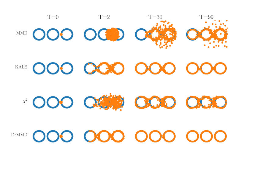
Figure 1: Animation of MMD, KALE, $\chi^{2}$ and DrMMD gradient descent on the Three-ring dataset.

8.2 Gradient flow for training student/teacher networks

Next, we consider a large-scale setting following Arbel et al. (2019), where a student network is trained to imitate the outputs of a teacher network. We consider a two-layer neural network of the form

$$\psi(z,x)=G\left(b^{1}+W^{1}\sigma\left(W^{0}z+b^{0}\right)\right),$$

where $\sigma$ is the ReLU non-linearity and $x$ is the concatenation of all network parameters $\left(b^{1},W^{1},b^{0},W^{0}\right)\in\mathbb{R}^{d}$. $G$ is an element-wise non-linear function $G:\mathbb{R}\to\mathbb{R},x\mapsto\exp(-\frac{1}{4}x^{2})$. The teacher network is of the form: $\Psi^{T}(z,\pi)=\int\psi(z,x)d\pi(x)$ where $\pi$ denotes the teacher distribution, and the student network is $\Psi^{S}(z,\mu)=\int\psi(z,x)d\mu(x)$ where $\mu$ denotes the student distribution. Here we consider Gaussian distributed $\mu$ and $\pi$ for simplicity. The student network can imitate the behavior of the teacher network by minimizing the objective

$$\min_{\mu\in\mathcal{P}_{2}(\mathbb{R}^{d})}\operatorname{\mathbb{E}}_{z\sim\mathbb{P}_{\text{data}}}\left(\Psi^{T}(z,\pi)-\Psi^{S}(z,\mu)\right)^{2},$$ (31)

where $\mathbb{P}_{\text{data}}$ is the distribution of the input data. If we define the kernel as the inner product of the neural network feature maps,

$$k(x,x^{\prime})=\operatorname{\mathbb{E}}_{z\sim\mathbb{P}_{\text{data}}}[\psi(z,x)^{\top}\psi(z,x^{\prime})],$$

then the objective of (31) can be equivalently expressed as

$$\min_{\mu\in\mathcal{P}_{2}(\mathbb{R}^{d})}\iint_{\mathcal{X}}k(x,x^{\prime})d(\pi-\mu)(x)d(\pi-\mu)(x^{\prime}),$$

which is precisely the $\operatorname{MMD}(\mu\|\pi)^{2}$ under the kernel $k$. Since $G(x)=\exp(-\frac{1}{4}x^{2})$, the kernel is bounded and so the $\operatorname{MMD}$ is well-defined. Also, since the kernel $k$ has bounded first and second-order derivatives, it satisfies the 2.

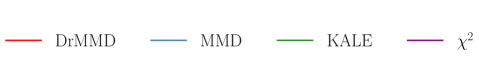
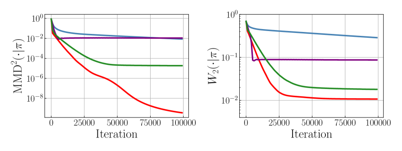
Figure 2: Left & Middle: Comparison of $\operatorname{DrMMD}$ descent with adaptive $\lambda$, $\operatorname{MMD}$ and $\operatorname{KALE}$ descent on three-ring synthetic data in terms of $\operatorname{MMD}$ and Wasserstein-2 distance with respect to the target $\pi$. Right: Comparison of MMD descent with and without noise injection, $\operatorname{DrMMD}$ descent with and without noise injection on training student/teacher networks in terms of validation $\operatorname{MMD}^{2}$ distance.

Therefore, the training of the student network with objective (31) can be treated as an optimization problem of $\operatorname{MMD}^{2}$ distance in $\mathcal{P}_{2}(\mathbb{R}^{d})$, i.e., as $\operatorname{MMD}$ gradient flow. It is shown in Arbel et al. (2019) that $\operatorname{MMD}$ flow and its descent scheme will generally get stuck in local optima because $\operatorname{MMD}$ is not geodesically convex, therefore noise injection has been proposed to escape these local optima.

With support from Theorems 4.1 and 5.1 on the convergence of $\operatorname{DrMMD}$ flow and its descent scheme, we propose to minimize $\operatorname{DrMMD}(\mu\|\pi)$ and use $\operatorname{DrMMD}$ descent rather than minimizing $\operatorname{MMD}(\mu\|\pi)^{2}$ directly. Although this does not directly minimize the objective in (31), the favorable convergence performance of $\operatorname{DrMMD}$ descent should result in a smaller $\operatorname{MMD}(\mu\|\pi)^{2}$ at convergence.

In our experimental setting, we are given $M=10$ particles $x^{(1)},\cdots,x^{(M)}$ from the teacher distribution $\pi=\mathcal{N}(0,\mathrm{I})$ and $N=1000$ particle $y_{0}^{(1)},\cdots,y_{0}^{(N)}$ from the initial student distribution $\mu_{0}=\mathcal{N}(0,10^{-3}\mathrm{I})$. The teacher particles are fixed while the student particles are updated according to Algorithm 1 at each time step. The initial (de)-regularization parameter is $\lambda_{0}=0.1$, the step size is $\gamma=0.1$, we apply a lower bound $\tilde{\lambda}=10^{-3}$, and the regularity $r$ is optimized over the set of $\{0.1,0.5,1.0\}$. For the architecture of the neural network, there are $3$ neurons in the hidden layer and the output dimension is $1$. The data distribution $\mathbb{P}_{\text{data}}$ is a uniform distribution on the sphere in $\mathbb{R}^{p}$ with $p=50$. $2000$ data are sampled from $\mathbb{P}_{\text{data}}$ with $1000$ as training dataset and another $1000$ as validation dataset. The kernel $k(x,x^{\prime})=\mathbb{E}_{z\sim\mathbb{P}_{\text{data}}}\left[\psi(z,x)^{\top}\psi\left(z,x^{\prime}\right)\right]$ is estimated by the average over $100$ randomly selected samples from the training dataset at each iteration. $\operatorname{DrMMD}$ and $\operatorname{MMD}$ descent stop after $n_{max}=15,000$ iterations when both converge. The final performance is evaluated in terms of $\operatorname{MMD}^{2}(\mu_{n_{max}}\|\pi)$ with kernel $k$ estimated by the average of $1000$ samples in the validation dataset.

In Figure 2 Right, we report the performance of $\operatorname{MMD}$ descent (with and without noise injection) along with the $\operatorname{DrMMD}$ descent (with and without noise injection) in terms of $\operatorname{MMD}$ distance on the validation dataset. We can see that the $\operatorname{DrMMD}$ descent does not get stuck in a local optimum, and leads to much lower validation $\operatorname{MMD}(\mu_{n_{max}}\|\pi)^{2}$ even without noise injection. We also run $\operatorname{DrMMD}$ descent with the noise injection scheme and find that noise injection can further improve the performance of $\operatorname{DrMMD}$ descent and outperforms $\operatorname{MMD}$ descent with noise injection. Although it is unclear whether the density ratio has enough regularity to meet the condition of 5.1, the kernel $k$ satisfies the boundedness and smoothness conditions of 2 and the target $\pi$ satisfies the Poincaré inequality since it is Gaussian. The $\operatorname{DrMMD}$ descent benefits from more favorable convergence properties which explains its superior performance.

The code to reproduce all the experiments can be found in the following GitHub repository. https://github.com/hudsonchen/DrMMD.

9 Discussion

In this paper, we introduced (de)-regularization of the MMD (called $\operatorname{DrMMD}$) and its associated Wasserstein gradient flow. As an interpolation between the $\operatorname{MMD}$ and $\chi^{2}$-divergence, the $\operatorname{DrMMD}$ gradient flow inherits strengths from both sides: it is easy to simulate in closed form with particles, and it has an exponential rate of convergence towards the global minimum up to a controllable barrier term when the target $\pi$ satisfies a Poincaré inequality. Additionally, we provide the optimal adaptive selection of a regularization coefficient that best balances the approximation and time discretization errors in $\operatorname{DrMMD}$ gradient descent. Our work is the first to prove theoretically that an adaptive kernel through adaptive regularization can result in improved convergence of MMD gradient flow. The theoretical results are consistent with the empirical evidence in several numerical experiments.

Following our work, there remain a number of interesting open problems. For example, (i) Since the kernel bandwidth has been known to play an important role in the performance of kernel-based algorithms, it is of interest to study the adaptive choice of kernel bandwidth in the context of $\operatorname{DrMMD}$ gradient flow. (ii) To generalize our convergence analysis to the Wasserstein gradient flow of all Moreau envelopes of $f$-divergences in reproducing kernel Hilbert space even when they do not have a closed-form expression as $\operatorname{DrMMD}$. (iii) While the current work proposes an approximation to the $\chi^{2}$-squared flow in the generative modeling setting, i.e., where the target distribution $\pi$ is known only through samples, it will be interesting to construct approximations to $\chi^{2}$-flow in the sampling setting, i.e., where $\pi$ is known in closed form (at least up to normalization).

10 Proofs

In this section, we present the proofs of the results presented in Sections 3–6.

10.1 Proof of 3.1

Note that

$$\operatorname{MMD}(\mu\|\pi)^{2} =\left\|m_{\mu}-m_{\pi}\right\|_{\mathcal{H}}^{2}=\left\|\int k(\cdot,x)d\mu(x)-\int k(\cdot,x)d\pi(x)\right\|_{\mathcal{H}}^{2}$$

$$=\left\|\int k(\cdot,x)\left(\frac{d\mu}{d\pi}(x)-1\right)\,d\pi(x)\right\|^{2}_{\mathcal{H}}=\left\|\iota^{*}_{\pi}\left(\frac{d\mu}{d\pi}-1\right)\right\|^{2}_{\mathcal{H}}$$

$$=\left\langle\mathcal{T}_{\pi}\left(\frac{d\mu}{d\pi}-1\right),\frac{d\mu}{d\pi}-1\right\rangle_{L^{2}(\pi)}=\left\|\mathcal{T}_{\pi}^{\frac{1}{2}}\left(\frac{d\mu}{d\pi}-1\right)\right\|_{L^{2}(\pi)}^{2}.$$

Also recall that the $\chi^{2}$-divergence between $\mu$ and $\pi$ is

$$\chi^{2}(\mu\|\pi)=\int\left(\frac{d\mu}{d\pi}-1\right)^{2}d\pi=\left\|\mathrm{I}\left(\frac{d\mu}{d\pi}-1\right)\right\|_{L^{2}(\pi)}^{2}.$$

10.2 Proof of 3.2

Let $\mu\ll\pi$. In order to prove the alternative form of $\operatorname{DrMMD}$ in (5), we start from (5) and show that it recovers (4).

$$\operatorname{DrMMD}(\mu||\pi) =(1+\lambda)\left\|\left(\Sigma_{\pi}+\lambda\mathrm{I}\right)^{-\frac{1}{2}}\left(m_{\mu}-m_{\pi}\right)\right\|_{\mathcal{H}}^{2}$$

$$=(1+\lambda)\left\|\left(\iota_{\pi}^{\ast}\iota_{\pi}+\lambda\mathrm{I}\right)^{-\frac{1}{2}}\iota_{\pi}^{\ast}\left(\frac{d\mu}{d\pi}-1\right)\right\|_{\mathcal{H}}^{2}$$

$$=(1+\lambda)\left\langle\left(\iota_{\pi}^{\ast}\iota_{\pi}+\lambda\mathrm{I}\right)^{-\frac{1}{2}}\iota_{\pi}^{\ast}\left(\frac{d\mu}{d\pi}-1\right),\left(\iota_{\pi}^{\ast}\iota_{\pi}+\lambda\mathrm{I}\right)^{-\frac{1}{2}}\iota_{\pi}^{\ast}\left(\frac{d\mu}{d\pi}-1\right)\right\rangle_{\mathcal{H}}$$

$$=(1+\lambda)\left\langle\iota_{\pi}\left(\iota_{\pi}^{\ast}\iota_{\pi}+\lambda\mathrm{I}\right)^{-1}\iota_{\pi}^{\ast}\left(\frac{d\mu}{d\pi}-1\right),\frac{d\mu}{d\pi}-1\right\rangle_{L^{2}(\pi)}$$

$$=(1+\lambda)\left\langle\iota_{\pi}\iota_{\pi}^{\ast}\left(\iota_{\pi}\iota_{\pi}^{\ast}+\lambda\mathrm{I}\right)^{-1}\left(\frac{d\mu}{d\pi}-1\right),\frac{d\mu}{d\pi}-1\right\rangle_{L^{2}(\pi)},$$ (32)

where the last equality follows by noticing $\iota_{\pi}\left(\iota_{\pi}^{*}\iota_{\pi}+\lambda\mathrm{I}\right)^{-1}\iota_{\pi}^{*}=\iota_{\pi}\iota_{\pi}^{*}\left(\iota_{\pi}\iota_{\pi}^{*}+\lambda\mathrm{I}\right)^{-1}$. Therefore,

$$\quad\operatorname{DrMMD}(\mu||\pi) =(1+\lambda)\left\langle\mathcal{T}_{\pi}\left(\mathcal{T}_{\pi}+\lambda\mathrm{I}\right)^{-1}\left(\frac{d\mu}{d\pi}-1\right),\frac{d\mu}{d\pi}-1\right\rangle_{L^{2}(\pi)}$$

$$=(1+\lambda)\left\|\left(\left(\mathcal{T}_{\pi}+\lambda\mathrm{I}\right)^{-1}\mathcal{T}_{\pi}\right)^{1/2}\left(\frac{d\mu}{d\pi}-1\right)\right\|_{L^{2}(\pi)}^{2},$$

which follows from the positivity and self-adjointness of $\mathcal{T}_{\pi}\left(\mathcal{T}_{\pi}+\lambda\mathrm{I}\right)^{-1}$. So (5) is proved. Next, we are going to prove the variational formulation in (6). Similarly, we start from (6) and show it recovers (4). Consider

$$\quad(1+\lambda)\sup_{h\in\mathcal{H}}\left\{\int h\mathrm{d}\mu-\int\left(\frac{h^{2}}{4}+h\right)\mathrm{d}\pi-\frac{\lambda}{4}\|h\|_{\mathcal{H}}^{2}\right\}$$

$$=-(1+\lambda)\inf_{h\in\mathcal{H}}\left\{\int\frac{h^{2}}{4}\mathrm{d}\pi-\int h(\mathrm{d}\mu-\mathrm{d}\pi)+\frac{\lambda}{4}\|h\|_{\mathcal{H}}^{2}\right\}$$

$$=-(1+\lambda)\inf_{h\in\mathcal{H}}\left\{\frac{1}{4}\left\langle h,\Sigma_{\pi}h\right\rangle_{\mathcal{H}}-\left\langle h,m_{\mu}-m_{\pi}\right\rangle_{\mathcal{H}}+\frac{\lambda}{4}\|h\|_{\mathcal{H}}^{2}\right\}$$

$$=-(1+\lambda)\inf_{h\in\mathcal{H}}\left\{\left\|\left(\frac{1}{4}\Sigma_{\pi}+\frac{\lambda}{4}\mathrm{I}\right)^{1/2}h-\frac{1}{2}\left(\frac{1}{4}\Sigma_{\pi}+\frac{\lambda}{4}\mathrm{I}\right)^{-1/2}(m_{\mu}-m_{\pi})\right\|_{\mathcal{H}}^{2}\right\}$$

$$\qquad\qquad+\frac{(1+\lambda)}{4}\left\|\left(\frac{1}{4}\Sigma_{\pi}+\frac{\lambda}{4}\mathrm{I}\right)^{-1/2}(m_{\mu}-m_{\pi})\right\|_{\mathcal{H}}^{2}.$$ (33)

The last equality follows from completing the squares, based on which it is easy to see that the infimum is achieved at $h_{\mu,\pi}^{\ast}=2\left(\Sigma_{\pi}+\lambda\mathrm{I}\right)^{-1}\left(m_{\mu}-m_{\pi}\right)$. For $\mu\ll\pi$, following the same derivations in (10.2), $h_{\mu,\pi}^{\ast}$ can be alternatively expressed as

$$h_{\mu,\pi}^{\ast}=2\left(\mathcal{T}_{\pi}+\lambda\mathrm{I}\right)^{-1}\mathcal{T}_{\pi}\left(\frac{d\mu}{d\pi}-1\right)$$ (34)

Plugging $h_{\mu,\pi}^{\ast}$ back into (33) recovers (4), so (6) is proved.

10.3 $\operatorname{DrMMD}$ is $\operatorname{MMD}$ with a regularized kernel $\tilde{k}$

Given the definition of $\tilde{k}(x,x^{\prime})=\left\langle\left(\Sigma_{\pi}+\lambda\mathrm{I}\right)^{-\frac{1}{2}}k(\cdot,x),\left(\Sigma_{\pi}+\lambda\mathrm{I}\right)^{-\frac{1}{2}}k(\cdot,x^{\prime})\right\rangle_{\mathcal{H}}$, it is clear that $\tilde{k}$ is symmetric and positive definite so it has a unique associated reproducing kernel Hilbert space $\tilde{\mathcal{H}}$ (Steinwart and Christmann, 2008, Theorem 4.21) with canonical feature map $\tilde{k}(x,\cdot)$. Therefore,

$$\quad\operatorname{DrMMD}(\mu\|\pi)$$

$$=(1+\lambda)\left\|\left(\Sigma_{\pi}+\lambda\mathrm{I}\right)^{-\frac{1}{2}}(m_{\mu}-m_{\pi})\right\|^{2}_{\mathcal{H}}$$

$$=(1+\lambda)\left\langle\left(\Sigma_{\pi}+\lambda\mathrm{I}\right)^{-\frac{1}{2}}\int k(x,\cdot)d\left(\pi-\mu\right)(x),\left(\Sigma_{\pi}+\lambda\mathrm{I}\right)^{-\frac{1}{2}}\int k(x^{\prime},\cdot)d\left(\pi-\mu\right)(x^{\prime})\right\rangle_{\mathcal{H}}$$

$$=(1+\lambda)\left\langle\int\left(\Sigma_{\pi}+\lambda\mathrm{I}\right)^{-\frac{1}{2}}k(x,\cdot)d\left(\pi-\mu\right)(x),\int\left(\Sigma_{\pi}+\lambda\mathrm{I}\right)^{-\frac{1}{2}}k(x^{\prime},\cdot)d\left(\pi-\mu\right)(x^{\prime})\right\rangle_{\mathcal{H}}$$

$$=(1+\lambda)\iint\left\langle\left(\Sigma_{\pi}+\lambda\mathrm{I}\right)^{-\frac{1}{2}}k(x,\cdot),\left(\Sigma_{\pi}+\lambda\mathrm{I}\right)^{-\frac{1}{2}}k(x^{\prime},\cdot)\right\rangle_{\mathcal{H}}d\left(\pi-\mu\right)(x)d\left(\pi-\mu\right)(x^{\prime})$$

$$=(1+\lambda)\iint\tilde{k}(x,x^{\prime})d\left(\pi-\mu\right)(x)d\left(\pi-\mu\right)(x^{\prime})$$

$$=(1+\lambda)\left\|\int\tilde{k}(x,\cdot)d(\mu-\pi)(x)\right\|^{2}_{\tilde{\mathcal{H}}}.$$

In the third and fourth equality above, we are using the fact that $\left(\Sigma_{\pi}+\lambda\mathrm{I}\right)^{-\frac{1}{2}}k(x,\cdot)\in\mathcal{H}$ is Bochner integrable and Bochner integral preserves inner product structure. So $\operatorname{DrMMD}$ is essentially $\operatorname{MMD}^{2}$ with a different kernel $\tilde{k}$ up to a multiplicative factor of $1+\lambda$.

Next, we present the Mercer decomposition of $\tilde{k}$. Notice that $\{e_{i}\}_{i\geq 1}$ are the eigenfunctions of $\mathcal{T}_{\pi}$, so $\{\sqrt{\varrho_{i}}e_{i}\}_{i\geq 1}$ are the eigenfunctions of $\Sigma_{\pi}$. For $x$ and $x^{\prime}$ in the support of $\pi$, $\tilde{k}$ also enjoys a pointwise convergent Mercer decomposition

$$\tilde{k}(x,x^{\prime}) =\left\langle\left(\Sigma_{\pi}+\lambda\mathrm{I}\right)^{-\frac{1}{2}}k(\cdot,x),\left(\Sigma_{\pi}+\lambda\mathrm{I}\right)^{-\frac{1}{2}}k(\cdot,x^{\prime})\right\rangle_{\mathcal{H}}$$

$$=\left\langle\left(\Sigma_{\pi}+\lambda\mathrm{I}\right)^{-\frac{1}{2}}\left(\sum_{i\geq 1}\varrho_{i}e_{i}(x)e_{i}\right),\left(\Sigma_{\pi}+\lambda\mathrm{I}\right)^{-\frac{1}{2}}\left(\sum_{i\geq 1}\varrho_{i}e_{i}(x^{\prime})e_{i}\right)\right\rangle_{\mathcal{H}}$$

$$=\left\langle\sum_{i\geq 1}\frac{\varrho_{i}}{\sqrt{\varrho_{i}+\lambda}}e_{i}(x)e_{i},\sum_{i\geq 1}\frac{\varrho_{i}}{\sqrt{\varrho_{i}+\lambda}}e_{i}(x^{\prime})e_{i}\right\rangle_{\mathcal{H}}$$

$$=\sum_{i\geq 1}\frac{\varrho_{i}}{\varrho_{i}+\lambda}e_{i}(x)e_{i}(x^{\prime}).$$ (35)

More properties of the regularized kernel $\tilde{k}$ are provided in B.3.

10.4 Proof of 3.3

Given that $\frac{d\mu}{d\pi}-1\in L^{2}(\pi)$, so

$$\operatorname{DrMMD}(\mu\|\pi)=(1+\lambda)\left\|\left(\left(\mathcal{T}_{\pi}+\lambda\mathrm{I}\right)^{-1}\mathcal{T}_{\pi}\right)^{1/2}\left(\frac{d\mu}{d\pi}-1\right)\right\|_{L^{2}(\pi)}^{2}\leq(1+\lambda)\left\|\frac{d\mu}{d\pi}-1\right\|_{L^{2}(\pi)}^{2}<\infty$$

for any $\lambda\geq 0$. We are allowed to interchange the limit and integration according to the dominated convergence theorem (Rudin, 1976) to achieve,

$$\lim_{\lambda\to 0}\operatorname{DrMMD}(\mu\|\pi)=\left\|\lim_{\lambda\to 0}\left(\left(\mathcal{T}_{\pi}+\lambda\mathrm{I}\right)^{-1}\mathcal{T}_{\pi}\right)^{1/2}\left(\frac{d\mu}{d\pi}-1\right)\right\|_{L^{2}(\pi)}^{2}=\left\|\frac{d\mu}{d\pi}-1\right\|_{L^{2}(\pi)}^{2}=\chi^{2}(\mu\|\pi).$$

From (5), we have that,

$$\sqrt{\operatorname{DrMMD}(\mu\|\pi)}=\sqrt{1+\lambda}\left\|\left(\Sigma_{\pi}+\lambda\mathrm{I}\right)^{-\frac{1}{2}}(m_{\mu}-m_{\pi})\right\|_{\mathcal{H}}$$

$$\leq\sqrt{1+\lambda}\left\|\left(\Sigma_{\pi}+\lambda\mathrm{I}\right)^{-\frac{1}{2}}\right\|_{op}\left\|m_{\mu}-m_{\pi}\right\|_{\mathcal{H}}\leq\sqrt{\frac{1+\lambda}{\lambda}}\times\operatorname{MMD}(\mu,\pi),$$ (36)

where the last inequality follows by noticing that $\Sigma_{\pi}=\iota_{\pi}^{\ast}\iota_{\pi}$ shares the same eigenvalues as $\mathcal{T}_{\pi}=\iota_{\pi}\iota_{\pi}^{\ast}$, and hence the eigenvalues of $(\Sigma_{\pi}+\lambda\mathrm{I})^{-1}$ are ${(\varrho_{i}+\lambda)}^{-1}$ which all smaller than $\frac{1}{\lambda}$. Therefore, $\operatorname{DrMMD}(\mu\|\pi)\leq\frac{1+\lambda}{\lambda}\operatorname{MMD}^{2}(\mu\|\pi)$.

On the other hand, using Lemma A.10 from (Hagrass et al., 2024), we have

$$\operatorname{MMD}\left(\mu\|\pi\right)=\left\|m_{\mu}-m_{\pi}\right\|_{\mathcal{H}}\leq\left\|(\Sigma_{\pi}+\lambda\mathrm{I}\right)^{\frac{1}{2}}\|_{op}\left\|\left(\Sigma_{\pi}+\lambda\mathrm{I}\right)^{-\frac{1}{2}}(m_{\mu}-m_{\pi})\right\|_{\mathcal{H}}$$

$$=\sqrt{\frac{1}{1+\lambda}}\left\|(\Sigma_{\pi}+\lambda\mathrm{I}\right)^{\frac{1}{2}}\|_{op}\sqrt{\operatorname{DrMMD}\left(\mu\|\pi\right)}\leq\sqrt{\frac{K+\lambda}{1+\lambda}}\sqrt{\operatorname{DrMMD}\left(\mu\|\pi\right)},$$ (37)

where $K$ is the upper bound on kernel $k$ in 2 and hence an upper bound on the operator norm of $\Sigma_{\pi}$. Combining (36) and (37), we have

$$\frac{1+\lambda}{K+\lambda}\operatorname{MMD}^{2}(\mu\|\pi)\leq\operatorname{DrMMD}\left(\mu\|\pi\right)\leq\frac{1+\lambda}{\lambda}\operatorname{MMD}^{2}(\mu\|\pi).$$

Therefore, $\lim_{\lambda\to\infty}\operatorname{DrMMD}(\mu\|\pi)=\operatorname{MMD}^{2}(\mu\|\pi)$, and the proposition is proved.

10.5 Proof of 3.4

In order to show that $\operatorname{DrMMD}$ is a probability divergence, we need to show that $\operatorname{DrMMD}$ enjoys non-negativity and definiteness. It is easy to see that $\operatorname{DrMMD}(\mu\|\pi)$ is non-negative from its definition in 1. Then, we prove definiteness, i.e., $\operatorname{DrMMD}(\mu||\pi)=0$ if and only if $\mu=\pi$. For the first direction, assume $\operatorname{DrMMD}(\mu\|\pi)=0$, so $\|(\Sigma_{\pi}+\lambda\mathrm{I})^{-1/2}\left(m_{\mu}-m_{\pi}\right)\|_{\mathcal{H}}^{2}=0$. Since $\left(\Sigma_{\pi}+\lambda\mathrm{I}\right)^{-1/2}$ is a non-singular operator, we must have that $m_{\mu}=m_{\pi}$ which implies $\mu=\pi$ as $k$ is $c_{0}$-universal and hence characteristic (Sriperumbudur et al., 2011). For the other direction, when $\mu=\pi$, immediately we can see $\operatorname{DrMMD}(\mu||\pi)=0$.

Then we prove that $\operatorname{DrMMD}$ metrizes weak convergence. For the first direction, we know from (36) that $\operatorname{DrMMD}(\mu_{n}\|\pi)\leq\frac{1+\lambda}{\lambda}\operatorname{MMD}^{2}(\mu_{n}\|\pi)$ and $\operatorname{MMD}^{2}(\mu_{n}\|\pi)\to 0$ as $\mu_{n}$ converges weakly to $\pi$ (Simon-Gabriel et al., 2023). For the converse direction, we assume that $\operatorname{DrMMD}\left(\mu_{n}\|\pi\right)\to 0$. From (37), we know that $\operatorname{MMD}^{2}\left(\mu\|\pi\right)\leq\frac{K+\lambda}{1+\lambda}\operatorname{DrMMD}\left(\mu\|\pi\right)$, therefore $\operatorname{DrMMD}\left(\mu_{n}\|\pi\right)\to 0$ implies $\operatorname{MMD}\left(\mu_{n}\|\pi\right)\to 0$, implying the weak convergence of $\mu_{n}$ to $\pi$, if $k$ is characteristic (Simon-Gabriel et al., 2023).

10.6 Proof of 4.1

In order to show that $\mathcal{F}_{\operatorname{DrMMD}}(\cdot)=\operatorname{DrMMD}(\cdot\|\pi)$ admits a well-defined gradient flow, we follow the same techniques in Proposition 7 of Glaser et al. (2021) and Lemma B.2 of Chizat and Bach (2018), where the key is to show that $(1+\lambda)\nabla h_{\mu,\pi}^{\ast}$ is the Fréchet subdifferential of $\mathcal{F}_{\operatorname{DrMMD}}$ evaluated at $\mu$.. According to Definition 10.1.1 of Ambrosio et al. (2005), it is equivalent to prove that, for any $\mu\in\mathcal{P}_{2}(\mathbb{R}^{d})$ and $\phi\in C_{c}^{\infty}(\mathbb{R}^{d})$,

$$\operatorname{DrMMD}\left((\mathrm{I}+\nabla\phi)_{\#}\mu\|\pi\right)-\operatorname{DrMMD}\left(\mu\|\pi\right)\geq(1+\lambda)\int\nabla\phi(x)^{\top}\nabla h_{\mu,\pi}^{\ast}(x)d\mu(x)$$

$$\qquad\qquad\qquad\qquad\qquad+o\left(\|\nabla\phi\|_{L^{2}(\mu)}\right).$$ (38)

Define $\rho_{t}=(\mathrm{I}+t\nabla\phi)_{\#}\mu$, $\varphi_{t}:\mathbb{R}^{d}\to\mathbb{R}^{d},x\mapsto x+t\nabla\phi(x)$ and $g(t)=\operatorname{DrMMD}(\rho_{t}||\pi)$. Then from B.6 we know that $g(t)$ is continuous and differentiable with respect to $t$ and

$$\frac{d}{dt}\Big{|}_{t=0}g(t)=(1+\lambda)\int\nabla\phi(x)^{\top}\nabla h_{\mu,\pi}^{\ast}(x)d\mu(x).$$

Since $t\mapsto g(t)$ is differentiable, using Taylor’s theorem and mean value theorem (Rudin, 1976), we know that there exists $0<\kappa<1$ such that

$$\quad\operatorname{DrMMD}\left((\mathrm{I}+\nabla\phi)_{\#}\mu\|\pi\right)-\operatorname{DrMMD}\left(\mu\|\pi\right)=g(1)-g(0)=\frac{d}{dt}\Big{|}_{t=0}g(t)+\frac{d^{2}}{dt^{2}}\Big{|}_{t=\kappa}g(t).$$

Therefore, to prove (10.6), the goal is to prove that $\frac{d^{2}}{dt^{2}}\big{|}_{t=\kappa}g(t)\geq o\left(\|\nabla\phi\|_{L^{2}(\mu)}\right)$. To this end, since we know from B.6 that $t\mapsto\frac{d}{dt}g(t)$ is continuous and differentiable, we have

$$\begin{aligned} &\quad\frac{d^{2}}{dt^{2}}\operatorname{DrMMD}(\rho_{t}||\pi)=2(1+\lambda)\iint\nabla\phi(x)^{\top}\nabla_{1}\nabla_{2}\tilde{k}\left(\varphi_{t}(x),\varphi_{t}(y)\right)\nabla\phi(y)d\mu(x)d\mu(y)\\ &+2(1+\lambda)\int\nabla\phi(x)^{\top}\left(\int\mathbf{H}_{1}\tilde{k}\left(\varphi_{t}(x),\varphi_{t}(y)\right)d\mu(y)-\int\mathbf{H}_{1}\tilde{k}\left(\varphi_{t}(x),y\right)d\pi(y)\right)\nabla\phi(x)d\mu(x),\end{aligned}$$

where $\tilde{k}$ is the regularized kernel defined in (7) and $\tilde{\mathcal{H}}$ is the associated RKHS. Using B.3, the first term above can be upper bounded by,

$$\quad\left|2(1+\lambda)\iint\nabla\phi(x)^{\top}\nabla_{1}\nabla_{2}\tilde{k}\left(\varphi_{t}(x),\varphi_{t}(y)\right)\nabla\phi(y)d\mu(x)d\mu(y)\right|$$

$$\leq 2(1+\lambda)\iint\left\|\nabla\phi(x)\right\|\left\|\nabla_{1}\nabla_{2}\tilde{k}\left(\varphi_{t}(x),\varphi_{t}(y)\right)\right\|_{F}\left\|\nabla\phi(y)\right\|d\mu(x)d\mu(y)$$

$$\leq 2(1+\lambda)\frac{K_{1d}}{\lambda}\left(\int\left\|\nabla\phi(y)\right\|d\mu(y)\right)^{2}\leq 2(1+\lambda)\frac{K_{1d}}{\lambda}\|\nabla\phi\|_{L^{2}(\mu)}^{2}.$$

Using B.3 again, the second term can be upper bounded by

$$\quad\left|\int\nabla\phi(x)^{\top}\left(\int\mathbf{H}_{1}\tilde{k}\left(\varphi_{t}(x),\varphi_{t}(y)\right)d\mu(y)-\int\mathbf{H}_{1}\tilde{k}\left(\varphi_{t}(x),y\right)d\pi(y)\right)\nabla\phi(x)d\mu(x)\right|$$

$$\leq\left|\int\nabla\phi(x)^{\top}\left(\int\mathbf{H}_{1}\tilde{k}\left(\varphi_{t}(x),\varphi_{t}(y)\right)d\mu(y)\right)\nabla\phi(x)d\mu(x)\right|$$

$$\qquad\qquad+\left|\int\nabla\phi(x)^{\top}\left(\int\mathbf{H}_{1}\tilde{k}\left(\varphi_{t}(x),y\right)d\pi(y)\right)\nabla\phi(x)d\mu(x)\right|$$

$$\leq\int\left\|\nabla\phi(x)\right\|\left(\int\left\|\mathbf{H}_{1}\tilde{k}\left(\varphi_{t}(x),\varphi_{t}(y)\right)\right\|_{F}d\mu(y)\right)\left\|\nabla\phi(x)\right\|d\mu(x)$$

$$\qquad\qquad+\int\left\|\nabla\phi(x)\right\|\left(\int\left\|\mathbf{H}_{1}\tilde{k}\left(\varphi_{t}(x),y\right)\right\|_{F}d\pi(y)\right)\left\|\nabla\phi(x)\right\|d\mu(x)$$

$$\leq 2\frac{\sqrt{KK_{2d}}}{\lambda}\|\nabla\phi\|_{L^{2}(\mu)}^{2}.$$

Combining the above two inequalities to have

$$\left|\frac{d^{2}}{dt^{2}}\operatorname{DrMMD}(\rho_{t}||\pi)\right|\leq 2(1+\lambda)\frac{K_{1d}}{\lambda}\|\nabla\phi\|_{L^{2}(\mu)}^{2}+4(1+\lambda)\frac{\sqrt{KK_{2d}}}{\lambda}\|\nabla\phi\|_{L^{2}(\mu)}^{2}.$$ (39)

Therefore, we have $\frac{d^{2}}{dt^{2}}\big{|}_{t=\kappa}g(t)=\mathcal{O}(\|\nabla\phi\|_{L^{2}(\mu)}^{2})=o(\|\nabla\phi\|_{L^{2}(\mu)})$ as $\|\nabla\phi\|_{L^{2}(\mu)}\to 0$. So (10.6) is proved, which means that $(1+\lambda)\nabla h_{\mu,\pi}^{\ast}(x)$ is the Fréchet subdifferential of $\mathcal{F}_{\operatorname{DrMMD}}$ evaluated at $\mu$. According to Definition 11.1.1 of Ambrosio et al. (2005), there exists a solution $(\mu_{t})_{t\geq 0}$ such that the following equation holds in the sense of distributions,

$$\partial_{t}\mu_{t}-(1+\lambda)\nabla\cdot\left(\mu_{t}\nabla h_{\mu_{t},\pi}^{\ast}\right)=0,$$

and such $(\mu_{t})_{t\geq 0}$ is indeed the $\operatorname{DrMMD}$ gradient flow, so existence is proved.

Next, we are going to prove uniqueness. (39) indicates that $\mathcal{F}_{\operatorname{DrMMD}}$ is geodesically $-(1+\lambda)\frac{4\sqrt{KK_{2d}}+2K_{1d}}{\lambda}$ semiconvex. Therefore the uniqueness of $(\mu_{t})_{t}$ follows from Theorem 11.2.1 of Ambrosio et al. (2005). (9) is proved in (39).

10.7 Proof of 4.2

Given $\mu\in\mathcal{P}_{2}\left(\mathbb{R}^{d}\right)$ and $\phi\in C_{c}^{\infty}\left(\mathbb{R}^{d}\right)$, consider the path $(\rho_{t})_{0\leq t\leq 1}$ from $\mu$ to $(\mathrm{I}+\nabla\phi)_{\#}\mu$ given by $\rho_{t}=(\mathrm{I}+t\nabla\phi)_{\#}\mu$. $(\rho_{t})_{0\leq t\leq 1}$ is a constant-time geodesic in the Wasserstein-2 space by construction (Appendix A: Further Background on $(\mathcal{P}_{2}(\mathbb{R}^{d}),W_{2})$). Define $\varphi_{t}:\mathbb{R}^{d}\to\mathbb{R}^{d},x\mapsto x+t\nabla\phi(x)$. We know from (Villani et al., 2009, Example 15.9) (by taking $m=2$) that,

$$\frac{d^{2}}{dt^{2}}\Big{|}_{t=0}\chi^{2}(\rho_{t}\|\pi) =\int\frac{d\mu}{d\pi}(x)\left(\nabla V(x)^{\top}\nabla\phi(x)-\nabla\cdot\nabla\phi(x)\right)^{2}d\mu(x)$$

$$\qquad+\int\frac{d\mu}{d\pi}(x)\nabla\phi(x)^{\top}\mathbf{H}V(x)\nabla\phi(x)d\mu(x)$$

$$\qquad\qquad+\int\frac{d\mu}{d\pi}(x)\left\|\mathbf{H}\phi(x)\right\|_{F}^{2}d\mu(x).$$ (40)

$V$ is twice differentiable, so $\nabla V$ as a function from $\mathbb{R}^{d}$ to $\mathbb{R}^{d}$ is continuous. $\phi\in C_{c}^{\infty}(\mathbb{R}^{d})$ has compact support, so $x\mapsto\nabla V(x)^{\top}\nabla\phi(x)-\nabla\cdot\nabla\phi(x)$ is a continuous function over a compact domain, so its image is also compact and hence bounded. Using similar arguments, $x\mapsto\nabla\phi(x)^{\top}\mathbf{H}V(x)\nabla\phi(x)$ and $x\mapsto\|\mathbf{H}\phi(x)\|_{F}^{2}$ are also continuous functions over compact domains, so they are all bounded.

Since $\frac{d\mu}{d\pi}-1\in\mathcal{H}\subset L^{2}(\pi)$ and $\int\frac{d\mu}{d\pi}(x)d\mu(x)=\|\frac{d\mu}{d\pi}-1\|_{L^{2}(\pi)}^{2}+1<\infty$, we have

$$\frac{d^{2}}{dt^{2}}\big{|}_{t=0}\chi^{2}(\rho_{t}\|\pi)<\infty.$$ (41)

Next, from B.9 we know that $\frac{d^{2}}{dt^{2}}\big{|}_{t=0}\chi^{2}(\rho_{t}\|\pi)$ can be alternatively expressed as,

$$\frac{d^{2}}{dt^{2}}\Big{|}_{t=0}\chi^{2}(\rho_{t}\|\pi) =2\int\left(\nabla\cdot\left(\nabla\phi(x)\mu(x)\right)\frac{1}{\pi(x)}\right)^{2}\pi(x)dx$$

$$\qquad\qquad+2\int\nabla\phi(x)^{\top}\mathbf{H}\left(\frac{\mu(x)}{\pi(x)}\right)\nabla\phi(x)\mu(x)dx.$$ (42)

Recall from B.6 that

$$\quad\frac{d^{2}}{dt^{2}}\Big{|}_{t=0}\operatorname{DrMMD}(\rho_{t}||\pi)$$

$$=2(1+\lambda)\iint\nabla\phi(x)^{\top}\nabla_{1}\nabla_{2}\tilde{k}\left(x,y\right)\nabla\phi(y)d\mu(x)d\mu(y)$$

$$\qquad+2(1+\lambda)\int\nabla\phi(x)^{\top}\left(\int\mathbf{H}_{1}\tilde{k}\left(x,y\right)d\mu(y)-\int\mathbf{H}_{1}\tilde{k}\left(x,y\right)d\pi(y)\right)\nabla\phi(x)d\mu(x).$$ (43)

In order to prove (10), our aim then is to compare and bound the difference of $\frac{d^{2}}{dt^{2}}\big{|}_{t=0}\chi^{2}(\rho_{t}\|\pi)$ in (10.7) and $\frac{1}{1+\lambda}\frac{d^{2}}{dt^{2}}\big{|}_{t=0}\operatorname{DrMMD}(\rho_{t}||\pi)$ in (10.7), so we compare and bound their first and second term separately.

The first term of (10.7) can be rewritten as

$$\int\left(\nabla\cdot(\nabla\phi(x)\mu(x))\frac{1}{\pi(x)}\right)^{2}\pi(x)dx=\sum_{i\geq 1}{\left\langle\nabla\cdot(\nabla\phi\mu)\frac{1}{\pi},e_{i}\right\rangle}_{\!L^{2}(\pi)}^{2}$$

$$=\sum_{i\geq 1}\left(\int\nabla\cdot\left(\nabla\phi(x)\mu(x)\right)e_{i}(x)dx\right)^{2}=\sum_{i\geq 1}\left(\int\nabla\phi(x)^{\top}\nabla e_{i}(x)\mu(x)dx\right)^{2},$$ (44)

where we use integration by parts in the last line since $\phi\in C_{c}^{\infty}(\mathbb{R}^{d})$. And the first term of (10.7) after rescaling by $\frac{1}{1+\lambda}$ can be rewritten as,

$$\quad 2\iint\nabla\phi(x)^{\top}\nabla_{1}\nabla_{2}\tilde{k}\left(x,y\right)\nabla\phi(y)d\mu(x)d\mu(y)$$

$$=2\iint\nabla\phi(x)^{\top}\nabla_{x}\nabla_{y}\left(\sum_{i\geq 1}\frac{\varrho_{i}}{\varrho_{i}+\lambda}e_{i}(x)e_{i}(y)\right)\nabla\phi(y)d\mu(x)d\mu(y)$$

$$=2\iint\Big{(}\nabla\cdot\left(\nabla\phi(x)\mu(x)\right)\Big{)}\Big{(}\nabla\cdot\left(\nabla\phi(y)\mu(y)\right)\Big{)}\sum_{i\geq 1}\frac{\varrho_{i}}{\varrho_{i}+\lambda}e_{i}(x)e_{i}(y)dxdy.$$ (45)

Since $\pi\ll\mathcal{L}^{d}$ so (10.3) is true for all $x,y\in\mathbb{R}^{d}$ hence the second equality is true, and the last equality uses integration by parts since $\phi\in C_{c}^{\infty}(\mathbb{R}^{d})$. Notice that

$$\quad\sum_{i\geq 1}\frac{\varrho_{i}}{\varrho_{i}+\lambda}\iint\left|e_{i}(x)e_{i}(y)\Big{(}\nabla\cdot(\nabla\phi(x)\mu(x))\Big{)}\Big{(}\nabla\cdot(\nabla\phi(y)\mu(y))\Big{)}\right|dxdy$$

$$=\sum_{i\geq 1}\frac{\varrho_{i}}{\varrho_{i}+\lambda}\left(\int\left|\Big{(}\nabla\cdot\left(\nabla\phi(x)\mu(x)\right)\Big{)}e_{i}(x)\right|dx\right)^{2}$$

$$\leq\frac{1}{\lambda}\sum_{i\geq 1}\varrho_{i}\left(\int\left(\frac{\nabla\cdot\left(\nabla\phi(x)\mu(x)\right)}{\mu(x)}\right)^{2}\mu(x)dx\right)\left(\int e_{i}(x)^{2}\mu(x)dx\right)$$

$$=\frac{1}{\lambda}\left(\int\left(\nabla\log\mu(x)^{\top}\nabla\phi(x)+\nabla\cdot\nabla\phi(x)\right)^{2}d\mu(x)\right)\left(\int\sum_{i\geq 1}\varrho_{i}e_{i}(x)^{2}d\mu(x)\right)$$

$$\leq\frac{K}{\lambda}\left(\int\left(\nabla\log\mu(x)^{\top}\nabla\phi(x)+\nabla\cdot\nabla\phi(x)\right)^{2}d\mu(x)\right)<+\infty.$$

The first inequality uses Cauchy-Schwartz, the second inequality uses $\sum_{i\geq 1}\varrho_{i}(e_{i}(x))^{2}=k(x,x)\leq K$. The last quantity is finite because $x\to\nabla\log\mu(x)$ is a continuous function and $\phi\in C_{c}^{\infty}(\mathbb{R}^{d})$ has compact support, hence the integral of a continuous function over a compact domain is always finite. Then, by using Fubini’s theorem (Rudin, 1976), we are allowed to interchange the infinite sum and integration of (45) to reach,

$$\quad 2\iint\Big{(}\nabla\cdot\left(\nabla\phi(x)\mu(x)\right)\Big{)}\Big{(}\nabla\cdot\left(\nabla\phi(y)\mu(y)\right)\Big{)}\sum_{i\geq 1}\frac{\varrho_{i}}{\varrho_{i}+\lambda}e_{i}(x)e_{i}(y)dxdy$$

$$=2\sum_{i\geq 1}\frac{\varrho_{i}}{\varrho_{i}+\lambda}\iint\Big{(}\nabla\cdot\left(\nabla\phi(x)\mu(x)\right)\Big{)}\Big{(}\nabla\cdot\left(\nabla\phi(y)\mu(y)\right)\Big{)}e_{i}(x)e_{i}(y)dxdy$$

$$=2\sum_{i\geq 1}\frac{\varrho_{i}}{\varrho_{i}+\lambda}\left(\int\Big{(}\nabla\cdot\left(\nabla\phi(x)\mu(x)\right)\Big{)}e_{i}(x)dx\right)^{2}$$

$$=2\sum_{i\geq 1}\frac{\varrho_{i}}{\varrho_{i}+\lambda}\left(\int\nabla\phi(x)^{\top}\nabla e_{i}(x)\mu(x)dx\right)^{2},$$

where the last equality uses integration by parts.

So the difference between the first term of (10.7) and (10.7) rescaled by $\frac{1}{1+\lambda}$ is,

$$\quad 2\left|\sum_{i\geq 1}\left(\int\nabla\phi(x)^{\top}\nabla e_{i}(x)\mu(x)dx\right)^{2}-\sum_{i\geq 1}\frac{\varrho_{i}}{\varrho_{i}+\lambda}\left(\int\nabla\phi(x)^{\top}\nabla e_{i}(x)\mu(x)dx\right)^{2}\right|$$

$$=2\sum_{i\geq 1}\frac{\lambda}{\varrho_{i}+\lambda}\left(\int\nabla\phi(x)^{\top}\nabla e_{i}(x)\mu(x)dx\right)^{2}.$$ (46)

Now we turn to the second term. The second term of (10.7) can be rewritten as

$$\quad 2\int\nabla\phi(x)^{\top}\mathbf{H}\left(\frac{d\mu}{d\pi}(x)\right)\nabla\phi(x)\mu(x)dx$$

$$=2\int\nabla\phi(x)^{\top}\mathbf{H}\left(\frac{d\mu}{d\pi}(x)-1\right)\nabla\phi(x)\mu(x)dx$$

$$=2\int\nabla\phi(x)^{\top}\mathbf{H}\left(\sum_{i\geq 1}{\left\langle\frac{d\mu}{d\pi}-1,e_{i}\right\rangle}_{\!L^{2}(\pi)}e_{i}(x)\right)\nabla\phi(x)\mu(x)dx,$$ (47)

and the second term of (10.7) rescaled by $\frac{1}{1+\lambda}$ can be rewritten as,

$$\quad 2\int\nabla\phi(x)^{\top}\left(\int\mathbf{H}_{1}\tilde{k}\left(x,y\right)d\mu(y)-\int\mathbf{H}_{1}\tilde{k}\left(x,y\right)d\pi(y)\right)\nabla\phi(x)d\mu(x)$$

$$=2\int\nabla\phi(x)^{\top}\mathbf{H}\left(\int\tilde{k}\left(x,y\right)d\mu(y)-\int\tilde{k}\left(x,y\right)d\pi(y)\right)\nabla\phi(x)d\mu(x)$$

$$=2\int\nabla\phi(x)^{\top}\mathbf{H}\left(\sum_{i\geq 1}\frac{\varrho_{i}}{\varrho_{i}+\lambda}e_{i}(x)\int e_{i}(y)d(\mu-\pi)(y)\right)\nabla\phi(x)d\mu(x)$$

$$=2\int\nabla\phi(x)^{\top}\mathbf{H}\left(\sum_{i\geq 1}\frac{\varrho_{i}}{\varrho_{i}+\lambda}{\left\langle\frac{d\mu}{d\pi}-1,e_{i}\right\rangle}_{\!L^{2}(\pi)}e_{i}(x)\right)\nabla\phi(x)d\mu(x).$$ (48)

Since $\pi\ll\mathcal{L}^{d}$ so (10.3) is true for all $x,y\in\mathbb{R}^{d}$ hence the third equality is true. From B.3, we have $\int\tilde{k}(x,y)d\mu(y)\leq\frac{K}{\lambda}$, $x\mapsto\tilde{k}(x,y)$ is second-order differentiable, $\sup_{x}|\mathbf{H}_{1}\tilde{k}(x,y)|\leq\frac{\sqrt{KK_{2d}}}{\lambda}$. So we are allowed to interchange integration and Hessian in the second equality using the differentiation lemma (Klenke, 2013, Theorem 6.28). Consider the difference of (48) and (47), we have

$$\quad 2\Bigg{|}\int\nabla\phi(x)^{\top}\mathbf{H}\left(\sum_{i\geq 1}{\left\langle\frac{d\mu}{d\pi}-1,e_{i}\right\rangle}_{\!L^{2}(\pi)}e_{i}(x)\right)\nabla\phi(x)\mu(x)dx$$

$$\qquad\qquad-\int\nabla\phi(x)^{\top}\mathbf{H}\left(\sum_{i\geq 1}\frac{\varrho_{i}}{\varrho_{i}+\lambda}{\left\langle\frac{d\mu}{d\pi}-1,e_{i}\right\rangle}_{\!L^{2}(\pi)}e_{i}(x)\right)\nabla\phi(x)d\mu(x)\Bigg{|}$$

$$=2\left|\int\nabla\phi(x)^{\top}\mathbf{H}\left(\sum_{i\geq 1}\frac{\lambda}{\varrho_{i}+\lambda}{\left\langle\frac{d\mu}{d\pi}-1,e_{i}\right\rangle}_{\!L^{2}(\pi)}e_{i}(x)\right)\nabla\phi(x)\mu(x)dx\right|.$$ (49)

Given $\frac{d\mu}{d\pi}-1\in\mathcal{H}$, there exists $q\in L^{2}(\pi)$ such that $\frac{d\mu}{d\pi}-1=\mathcal{T}^{1/2}_{\pi}q$ so that $\langle\frac{d\mu}{d\pi}-1,e_{i}\rangle=\varrho_{i}^{1/2}\langle q,e_{i}\rangle$ for all $i$. For $j,r\in\{1,\cdots,d\}$, we have

$$g_{M_{0}}(x) :=\left|\sum_{i\geq M_{0}}\frac{\lambda}{\varrho_{i}+\lambda}{\left\langle\frac{d\mu}{d\pi}-1,e_{i}\right\rangle}_{\!L^{2}(\pi)}\partial_{j}\partial_{r}e_{i}(x)\right|=\left|\sum_{i\geq M_{0}}\frac{\lambda}{\varrho_{i}+\lambda}\varrho_{i}^{1/2}{\left\langle q,e_{i}\right\rangle}_{\!L^{2}(\pi)}\partial_{j}\partial_{r}e_{i}(x)\right|$$

$$\leq\left(\sum_{i\geq M_{0}}\left(\frac{\lambda}{\varrho_{i}+\lambda}\right)^{2}{\left\langle q,e_{i}\right\rangle}_{\!L^{2}(\pi)}^{2}\right)^{1/2}\left(\sum_{i\geq M_{0}}\varrho_{i}\left(\partial_{j}\partial_{r}e_{i}(x)\right)^{2}\right)^{1/2}$$

$$\leq\left(\sum_{i\geq M_{0}}{\left\langle q,e_{i}\right\rangle}_{\!L^{2}(\pi)}^{2}\right)^{1/2}\left(\sum_{i\geq M_{0}}\varrho_{i}\left(\partial_{j}\partial_{r}e_{i}(x)\right)^{2}\right)^{1/2}\leq\sqrt{K_{2d}}\left(\sum_{i\geq M_{0}}{\left\langle q,e_{i}\right\rangle}_{\!L^{2}(\pi)}^{2}\right)^{1/2}.$$

The final inequality holds because,

$$\sum_{j,r=1}^{d}\sum_{i\geq 1}\varrho_{i}\left(\partial_{j}\partial_{r}e_{i}(x)\right)^{2} \leq\sum_{j,r=1}^{d}\sum_{i\geq 1}\varrho_{i}{\left\langle\partial_{j}\partial_{r}k(x,\cdot),e_{i}\right\rangle}_{\!\mathcal{H}}^{2}=\sum_{j,r=1}^{d}\sum_{i\geq 1}{\left\langle\partial_{j}\partial_{r}k(x,\cdot),\sqrt{\varrho_{i}}e_{i}\right\rangle}_{\!\mathcal{H}}^{2}$$

$$=\sum_{j,r=1}^{d}\left\|\partial_{j}\partial_{r}k(x,\cdot)\right\|_{\mathcal{H}}^{2}=\left\|\mathbf{H}_{1}k(x,\cdot)\right\|_{\mathcal{H}^{d\times d}}^{2}\leq K_{2d}.$$ (50)

Since $\left\|q\right\|_{L^{2}(\pi)}$ is bounded, so $\sum_{i\geq M_{0}}{\left\langle q,e_{i}\right\rangle}_{\!L^{2}(\pi)}^{2}$ converges to $0$ uniformly as $M_{0}\to\infty$ and hence $g_{M_{0}}(x)$ converge to $0$ uniformly. Therefore we are allowed to interchange the Hessian and the infinite sum (Rudin, 1976) in (49) to achieve,

$$\quad 2\left|\int\nabla\phi(x)^{\top}\mathbf{H}\left(\sum_{i\geq 1}\frac{\lambda}{\varrho_{i}+\lambda}{\left\langle\frac{d\mu}{d\pi}-1,e_{i}\right\rangle}_{\!L^{2}(\pi)}e_{i}(x)\right)\nabla\phi(x)\mu(x)dx\right|$$

$$=2\left|\int\nabla\phi(x)^{\top}\left(\sum_{i\geq 1}\frac{\lambda}{\varrho_{i}+\lambda}\varrho_{i}^{1/2}{\left\langle q,e_{i}\right\rangle}_{\!L^{2}(\pi)}\mathbf{H}e_{i}(x)\right)\nabla\phi(x)\mu(x)dx\right|$$

$$\leq 2\left(\sum_{i\geq 1}\left(\frac{\lambda}{\varrho_{i}+\lambda}\right)^{2}{\left\langle q,e_{i}\right\rangle}_{\!L^{2}(\pi)}^{2}\right)^{1/2}\left(\sum_{i\geq 1}\varrho_{i}\left(\int\nabla\phi(x)^{\top}\mathbf{H}e_{i}(x)\nabla\phi(x)\mu(x)dx\right)^{2}\right)^{1/2}$$

$$\leq 2\left(\sum_{i\geq 1}\left(\frac{\lambda}{\varrho_{i}+\lambda}\right)^{2}{\left\langle q,e_{i}\right\rangle}_{\!L^{2}(\pi)}^{2}\right)^{1/2}\left(\sum_{i\geq 1}\varrho_{i}\left\|\mathbf{H}e_{i}(x)\right\|_{op}^{2}\left(\int\nabla\phi(x)^{\top}\nabla\phi(x)\mu(x)dx\right)^{2}\right)^{1/2}$$

$$\leq 2\left(\sum_{i\geq 1}\left(\frac{\lambda}{\varrho_{i}+\lambda}\right)^{2}{\left\langle q,e_{i}\right\rangle}_{\!L^{2}(\pi)}^{2}\right)^{1/2}\left(\sum_{i\geq 1}\varrho_{i}\left\|\mathbf{H}e_{i}(x)\right\|_{op}^{2}\right)^{1/2}\|\nabla\phi\|_{L^{2}(\mu)}^{2}$$

$$\leq 2\left(\sum_{i\geq 1}\left(\frac{\lambda}{\varrho_{i}+\lambda}\right)^{2}{\left\langle q,e_{i}\right\rangle}_{\!L^{2}(\pi)}^{2}\right)^{1/2}\left(\sum_{i\geq 1}\varrho_{i}\left\|\mathbf{H}e_{i}(x)\right\|_{F}^{2}\right)^{1/2}\|\nabla\phi\|_{L^{2}(\mu)}^{2}$$

$$\leq 2\left(\sum_{i\geq 1}\left(\frac{\lambda}{\varrho_{i}+\lambda}\right)^{2}{\left\langle q,e_{i}\right\rangle}_{\!L^{2}(\pi)}^{2}\right)^{1/2}\sqrt{K_{2d}}\|\nabla\phi\|_{L^{2}(\mu)}^{2}.$$ (51)

The first inequality uses Cauchy Schwartz, the second last inequality uses that matrix operator norm is smaller than matrix Frobenius norm, and the last inequality uses (10.7). Combining together (46) and (51), we reach

$$\quad\left|\frac{1}{1+\lambda}\frac{d^{2}}{dt^{2}}\Big{|}_{t=0}\operatorname{DrMMD}(\rho_{t}||\pi)-\frac{d^{2}}{dt^{2}}\Big{|}_{t=0}\chi^{2}(\rho_{t}||\pi)\right|$$

$$\leq 2\sum_{i\geq 1}\frac{\lambda}{\varrho_{i}+\lambda}\left(\int\nabla\phi(x)^{\top}\nabla e_{i}(x)\mu(x)dx\right)^{2}$$

$$\qquad\qquad+2\left(\sum_{i\geq 1}\left(\frac{\lambda}{\varrho_{i}+\lambda}\right)^{2}{\left\langle q,e_{i}\right\rangle}_{\!L^{2}(\pi)}^{2}\right)^{1/2}\sqrt{K_{2d}}\|\nabla\phi\|_{L^{2}(\mu)}^{2}$$

$$=:\bar{R}(\lambda,\mu,\nabla\phi).$$

Therefore,

$$\frac{d^{2}}{dt^{2}}\Big{|}_{t=0}\operatorname{DrMMD}(\rho_{t}||\pi) \geq(1+\lambda)\frac{d^{2}}{dt^{2}}\Big{|}_{t=0}\chi^{2}(\rho_{t}||\pi)-(1+\lambda)\bar{R}(\lambda,\mu,\nabla\phi)$$

$$\geq(1+\lambda)\int\frac{d\mu}{d\pi}(x)\nabla\phi(x)^{\top}\mathbf{H}V(x)\nabla\phi(x)d\mu(x)-(1+\lambda)\bar{R}(\lambda,\mu,\nabla\phi)$$

$$\geq(1+\lambda)\alpha\int\frac{d\mu}{d\pi}(x)\|\nabla\phi(x)\|^{2}d\mu(x)-(1+\lambda)\bar{R}(\lambda,\mu,\nabla\phi),$$

where the second inequality is using (10.7) and the last inequality is using $\mathbf{H}V\succeq\alpha\mathrm{I}$. So (10) is proved.

Define $R(\lambda,\mu,\nabla\phi):=(1+\lambda)\bar{R}(\lambda,\mu,\nabla\phi)$. The final thing left to check is $\lim_{\lambda\to 0}R(\lambda,\mu,\nabla\phi)=0$, which is equivalent to check that $\lim_{\lambda\to 0}\bar{R}(\lambda,\mu,\nabla\phi)=0$. Since we know from (41) and (44) that

$$\sum_{i\geq 1}\left(\int\nabla\phi(x)^{\top}\nabla e_{i}(x)\mu(x)dx\right)^{2}<\frac{d^{2}}{dt^{2}}\Big{|}_{t=0}\chi^{2}(\rho_{t}\|\pi)<\infty,$$

using dominated convergence theorem (Rudin, 1976) we are allowed to interchange infinite sum and taking limits,

$$\lim_{\lambda\to 0}\sum_{i\geq 1}\frac{\lambda}{\varrho_{i}+\lambda}\left(\int\nabla\phi(x)^{\top}\nabla e_{i}(x)\mu(x)dx\right)^{2} =\sum_{i\geq 1}\lim_{\lambda\to 0}\frac{\lambda}{\varrho_{i}+\lambda}\left(\int\nabla\phi(x)^{\top}\nabla e_{i}(x)\mu(x)dx\right)^{2}$$

$$=0.$$

Similarly, because $\sum_{i\geq 1}\left(\frac{\lambda}{\varrho_{i}+\lambda}\right)^{2}{\left\langle q,e_{i}\right\rangle}_{\!L^{2}(\pi)}^{2}<\left\|q\right\|_{L^{2}(\pi)}^{2}<\infty$, using dominated convergence theorem (Rudin, 1976) again, we have,

$$\lim_{\lambda\to 0}\sum_{i\geq 1}\left(\frac{\lambda}{\varrho_{i}+\lambda}\right)^{2}{\left\langle q,e_{i}\right\rangle}_{\!L^{2}(\pi)}^{2}=\sum_{i\geq 1}\lim_{\lambda\to 0}\left(\frac{\lambda}{\varrho_{i}+\lambda}\right)^{2}{\left\langle q,e_{i}\right\rangle}_{\!L^{2}(\pi)}^{2}=0.$$

Therefore, we have that

$$\lim_{\lambda\to 0}R(\lambda,\mu,\nabla\phi)=\lim_{\lambda\to 0}\bar{R}(\lambda,\mu,\nabla\phi)=0.$$

And the proof of the proposition is finished.

10.8 Proof of 4.1

Considering the time derivative of $\operatorname{KL}(\mu_{t}\|\pi)$, we have

$$\quad\frac{d}{dt}\operatorname{KL}(\mu_{t}\|\pi)$$

$$=-(1+\lambda)\int\nabla h_{\mu_{t},\pi}^{\ast}(x)^{\top}\nabla\log\frac{d\mu_{t}}{d\pi}(x)\mu_{t}(x)dx$$

$$=-(1+\lambda)\int\nabla h_{\mu_{t},\pi}^{\ast}(x)^{\top}\nabla\frac{d\mu_{t}}{d\pi}(x)\pi(x)dx$$

$$=-(1+\lambda)\int\left(\nabla h_{\mu_{t},\pi}^{\ast}(x)-2\nabla\frac{d\mu_{t}}{d\pi}(x)\right)^{\top}\nabla\frac{d\mu_{t}}{d\pi}(x)\pi(x)dx-2(1+\lambda)\int\pi(x)\left\|\nabla\frac{d\mu_{t}}{d\pi}(x)\right\|^{2}dx$$

$$=-(1+\lambda)\int\left(\nabla h_{\mu_{t},\pi}^{\ast}(x)-2\nabla\left(\frac{d\mu_{t}}{d\pi}(x)-1\right)\right)^{\top}\nabla\frac{d\mu_{t}}{d\pi}(x)\pi(x)dx$$

$$-2(1+\lambda)\int\pi(x)\left\|\nabla\frac{d\mu_{t}}{d\pi}(x)\right\|^{2}dx.$$ (52)

Case one: $\int\pi(x)\left\|\nabla\frac{d\mu_{t}}{d\pi}(x)\right\|^{2}dx<\infty$.

We use integration by parts for the first term in (52) and we can safely ignore the boundary term due to condition 5 that for $i=1,\ldots,d$, $\lim\limits_{x\to\infty}\left(h_{\mu_{t},\pi}^{\ast}(x)-2\frac{d\mu_{t}}{d\pi}(x)\right)\left(\partial_{i}\frac{d\mu_{t}}{d\pi}(x)\right)\pi(x)\to 0$. So, we obtain

$$\quad\frac{d}{dt}\operatorname{KL}(\mu_{t}\|\pi)=(1+\lambda)\int\left(h_{\mu_{t},\pi}^{\ast}(x)-2\left(\frac{d\mu_{t}}{d\pi}(x)-1\right)\right)\nabla\cdot\left(\pi(x)\nabla\frac{d\mu_{t}}{d\pi}(x)\right)dx$$

$$\qquad\qquad-2(1+\lambda)\int\pi(x)\left\|\nabla\frac{d\mu_{t}}{d\pi}(x)\right\|^{2}dx$$

$$=(1+\lambda)\int\left(h_{\mu_{t},\pi}^{\ast}(x)-2\left(\frac{d\mu_{t}}{d\pi}(x)-1\right)\right)\frac{\nabla\cdot\left(\pi(x)\nabla\frac{d\mu_{t}}{d\pi}(x)\right)}{\pi(x)}\pi(x)dx$$

$$\qquad\qquad-2(1+\lambda)\int\pi(x)\left\|\nabla\frac{d\mu_{t}}{d\pi}(x)\right\|^{2}dx$$

$$\leq(1+\lambda)\left\|h_{\mu_{t},\pi}^{\ast}-2\left(\frac{d\mu_{t}}{d\pi}-1\right)\right\|_{L^{2}(\pi)}\left\|\frac{\nabla\cdot\left(\pi\nabla\frac{d\mu_{t}}{d\pi}\right)}{\pi}\right\|_{L^{2}(\pi)}-\frac{2(1+\lambda)}{C_{P}}\operatorname{KL}(\mu_{t}\|\pi),$$ (53)

where the first part of the last inequality holds by using Cauchy Schwartz, and the second part holds by the fact that $\operatorname{KL}(\mu_{t}\|\pi)\leq\chi^{2}(\mu_{t}\|\pi)$ (Van Erven and Harremos, 2014) and by applying the Poincaré inequality with $f=\frac{d\mu_{t}}{d\pi}-1$ (notice that $\|\nabla f\|_{L^{2}(\pi)}<\infty$ from Case one and $\|f\|_{L^{2}(\pi)}<\infty$ from condition 3),

$$\int\pi(x)\left\|\nabla\frac{d\mu_{t}}{d\pi}(x)\right\|^{2}dx\geq\frac{1}{C_{P}}\chi^{2}(\mu_{t}\|\pi)\geq\frac{1}{C_{P}}\operatorname{KL}(\mu_{t}\|\pi).$$ (54)

Since $\frac{d\mu_{t}}{d\pi}-1\in\operatorname{Ran}\left(\mathcal{T}_{\pi}^{r}\right)$ with $r>0$, using B.5 we have

$$\left\|h_{\mu_{t},\pi}^{\ast}-2\left(\frac{d\mu_{t}}{d\pi}-1\right)\right\|_{L^{2}(\pi)}\leq 2\lambda^{r}\left\|q_{t}\right\|_{L^{2}(\pi)}.$$ (55)

Then, notice that

$$\left\|\frac{\nabla\cdot\left(\pi\nabla\frac{d\mu_{t}}{d\pi}\right)}{\pi}\right\|_{L^{2}(\pi)}^{2}=\int\frac{\left[\nabla\cdot\left(\pi(x)\nabla\frac{d\mu_{t}}{d\pi}(x)\right)\right]^{2}}{\pi(x)^{2}}d\pi(x)$$

$$=\int\frac{\left(\nabla\pi(x)^{\top}\nabla\frac{d\mu_{t}}{d\pi}(x)+\pi(x)\nabla\cdot\nabla\frac{d\mu_{t}}{d\pi}(x)\right)^{2}}{\pi(x)^{2}}d\pi(x)$$

$$=\int\left(\nabla\log\pi(x)^{\top}\nabla\frac{d\mu_{t}}{d\pi}(x)+\Delta\frac{d\mu_{t}}{d\pi}(x)\right)^{2}d\pi(x)$$

$$\leq\int 2\left(\nabla\log\pi(x)^{\top}\nabla\frac{d\mu_{t}}{d\pi}(x)\right)^{2}+2\left(\Delta\frac{d\mu_{t}}{d\pi}(x)\right)^{2}d\pi(x)$$

$$=2\left\|\nabla\left(\log\pi\right)^{\top}\nabla\left(\frac{d\mu_{t}}{d\pi}\right)\right\|_{L^{2}(\pi)}^{2}+2\left\|\Delta\left(\frac{d\mu_{t}}{d\pi}\right)\right\|_{L^{2}(\pi)}^{2}\leq 2\mathcal{J}_{t}^{2}+2\mathcal{I}_{t}^{2}.$$ (56)

Therefore, plugging (55) and (56) back to (53), we have

$$\frac{d}{dt}\operatorname{KL}(\mu_{t}\|\pi)\leq 4(1+\lambda)\lambda^{r}\left\|q_{t}\right\|_{L^{2}(\pi)}\left(\mathcal{J}_{t}+\mathcal{I}_{t}\right)-\frac{2(1+\lambda)}{C_{P}}\operatorname{KL}(\mu_{t}\|\pi).$$ (57)

Case two: $\int\pi(x)\left\|\nabla\frac{d\mu_{t}}{d\pi}(x)\right\|^{2}dx=\infty$.

The first term of (52) remains the same, and the second term of (52) now equals infinity which is larger than the finite $\frac{2(1+\lambda)}{C_{P}}\operatorname{KL}(\mu_{t}\|\pi)$, so we also obtain (57) as in Case one.

Therefore, both Case one and Case two result in (57). Using the Gronwall lemma, we obtain that for any $T>0$,

$$\begin{aligned} \operatorname{KL}(\mu_{T}\|\pi)&\leq\exp\left(-\frac{2(1+\lambda)}{C_{P}}T\right)\operatorname{KL}(\mu_{0}\|\pi)\\ &+4(1+\lambda)\lambda^{r}\int_{0}^{T}\exp\left(-\frac{2(1+\lambda)}{C_{P}}(T-t)\right)\left\|q_{t}\right\|_{L^{2}(\pi)}(\mathcal{J}_{t}+\mathcal{I}_{t})dt,\end{aligned}$$

which concludes the proof of 4.1.

Derivation of (16) under stronger range assumption $r=\frac{1}{2}$.

Notice that for any $x\in\mathbb{R}^{d}$, since $k$ is differentiable

$$\nabla\left(\frac{d\mu_{t}}{d\pi}-1\right)(x)=\left\langle\nabla k(x,\cdot),\frac{d\mu_{t}}{d\pi}-1\right\rangle_{\mathcal{H}^{d}}\leq\sqrt{K_{1d}}\left\|\frac{d\mu_{t}}{d\pi}-1\right\|_{\mathcal{H}}.$$

And since $\frac{d\mu_{t}}{d\pi}-1\in\mathcal{H}$, there exists $q_{t}\in L^{2}(\pi)$ such that $\left\langle\frac{d\mu_{t}}{d\pi}-1,e_{i}\right\rangle_{L^{2}(\pi)}=\varrho_{i}^{1/2}\left\langle q_{t},e_{i}\right\rangle_{L^{2}(\pi)}$ for all $i$, so

$$\left\|\frac{d\mu_{t}}{d\pi}-1\right\|_{\mathcal{H}}^{2}=\sum_{i\geq 1}\frac{1}{\varrho_{i}}\left\langle\frac{d\mu_{t}}{d\pi}-1,e_{i}\right\rangle_{L^{2}(\pi)}^{2}=\sum_{i\geq 1}\left\langle q_{t},e_{i}\right\rangle_{L^{2}(\pi)}^{2}=\|q_{t}\|_{L^{2}(\pi)}^{2}.$$

Combining the above two equations, we have

$$\left\|\nabla\left(\log\pi\right)^{\top}\nabla\left(\frac{d\mu_{t}}{d\pi}-1\right)\right\|_{L^{2}(\pi)}\leq\sqrt{K_{1d}}\|q_{t}\|_{L^{2}(\pi)}\left\|\nabla\log\pi\right\|_{L^{2}(\pi)}.$$

Also, for the other one, notice that

$$\Delta\left(\frac{d\mu_{t}}{d\pi}\right)(x) \leq\left\|\mathbf{H}\left(\frac{d\mu_{t}}{d\pi}-1\right)(x)\right\|_{F}=\left\|\left\langle\mathbf{H}k(x,\cdot),\frac{d\mu_{t}}{d\pi}-1\right\rangle\right\|_{F}$$

$$\leq\left\|\mathbf{H}k(x,\cdot)\right\|_{\mathcal{H}^{d\times d}}\left\|\frac{d\mu_{t}}{d\pi}-1\right\|_{\mathcal{H}}\leq\sqrt{K_{2d}}\|q_{t}\|_{L^{2}(\pi)}.$$

Therefore,

$$\left\|\Delta\left(\frac{d\mu_{t}}{d\pi}\right)\right\|_{L^{2}(\pi)}\leq\sqrt{K_{2d}}\|q_{t}\|_{L^{2}(\pi)}.$$

10.9 Proof of 5.1

We know that $\mu_{n+1}=(\mathrm{I}-\gamma(1+\lambda)\nabla h)_{\#}\mu_{n}$ where we drop the subscripts of the witness function $h_{\mu_{n},\pi}$ when it causes no ambiguity. Denote $\rho_{t}=(\mathrm{I}-t(1+\lambda)\nabla h)_{\#}\mu_{n}$, so $\rho_{0}=\mu_{n}$, and $\rho_{\gamma}=\mu_{n+1}$. Consider the difference of KL divergence between the two iterates $\mu_{n+1}$ and $\mu_{n}$ along the time-discretized $\operatorname{DrMMD}$ flow:

$$\operatorname{KL}(\mu_{n+1}\|\pi)-\operatorname{KL}(\mu_{n}\|\pi) =\operatorname{KL}(\rho_{\gamma}\|\pi)-\operatorname{KL}(\rho_{0}\|\pi)$$

$$=\frac{d}{dt}\Big{|}_{t=0}\operatorname{KL}(\rho_{t}\|\pi)\gamma+\int_{0}^{\gamma}(\gamma-t)\frac{d^{2}}{dt^{2}}\operatorname{KL}(\rho_{t}\|\pi)dt.$$ (58)

For the first term of (58),

$$\quad\frac{d}{dt}\Big{|}_{t=0}\operatorname{KL}(\rho_{t}\|\pi)$$

$$=-(1+\lambda)\operatorname{\mathbb{E}}_{\mu_{n}}\left[\nabla\log\frac{d\mu_{n}}{d\pi}^{\top}\nabla h\right]=-(1+\lambda)\operatorname{\mathbb{E}}_{\pi}\left[\nabla\frac{d\mu_{n}}{d\pi}^{\top}\nabla h\right]$$

$$=-2(1+\lambda)\left\|\nabla\frac{d\mu_{n}}{d\pi}\right\|_{L^{2}(\pi)}^{2}+(1+\lambda)\operatorname{\mathbb{E}}_{\pi}\left[\nabla\frac{d\mu_{n}}{d\pi}^{\top}\left(2\nabla\frac{d\mu_{n}}{d\pi}-\nabla h\right)\right]$$

$$=-2(1+\lambda)\left\|\nabla\frac{d\mu_{n}}{d\pi}\right\|_{L^{2}(\pi)}^{2}+(1+\lambda)\int\left(\nabla\frac{d\mu_{n}}{d\pi}(x)\right)^{\top}\left(2\nabla\left(\frac{d\mu_{n}}{d\pi}(x)-1\right)-\nabla h(x)\right)\pi(x)dx$$

$$=-2(1+\lambda)\left\|\nabla\frac{d\mu_{n}}{d\pi}\right\|_{L^{2}(\pi)}^{2}-(1+\lambda)\int\left(2\left(\frac{d\mu_{n}}{d\pi}(x)-1\right)-h(x)\right)\nabla\cdot\left(\pi(x)\nabla\frac{d\mu_{n}}{d\pi}(x)\right)dx$$

$$\leq-(1+\lambda)\frac{2}{C_{P}}\chi^{2}(\mu_{n}\|\pi)+(1+\lambda)\left\|h-2\left(\frac{d\mu_{n}}{d\pi}-1\right)\right\|_{L^{2}(\pi)}\left\|\frac{\nabla\cdot\left(\pi\nabla\frac{d\mu_{n}}{d\pi}\right)}{\pi}\right\|_{L^{2}(\pi)},$$ (59)

where the fourth equality uses an integration by parts, and the last inequality uses Poincaré inequality for the first term under similar arguments in Section 10.8 and uses Cauchy-Schwartz for the second term. Using B.5 and the derivations in (56), (10.9) can be further upper bounded by

$$\frac{d}{dt}\Big{|}_{t=0}\operatorname{KL}(\rho_{t}\|\pi)\leq-(1+\lambda)\frac{2}{C_{P}}\chi^{2}(\mu_{n}\|\pi)+2(1+\lambda)\lambda^{r}Q\left(\mathcal{J}+\mathcal{I}\right).$$ (60)

Then, for the second term of (58), we know from Example 15.9 of Villani et al. (2009) (taking $m=1$) that,

$$\frac{d^{2}}{dt^{2}}\operatorname{KL}(\rho_{t}\|\pi) =(1+\lambda)^{2}\int\nabla h(x)^{\top}\mathbf{H}V(\varphi_{t}(x))\nabla h(x)d\mu_{n}(x)$$

$$+(1+\lambda)^{2}\int\left\|\mathbf{H}h(x)\left(\mathrm{I}-t(1+\lambda)\mathbf{H}h(x)\right)^{-1}\right\|_{F}^{2}d\mu_{n}(x).$$

Because $2(1+\lambda)\gamma\sqrt{\chi^{2}\left(\mu_{0}\|\pi\right)\frac{K_{2d}}{\lambda}}\leq\frac{\zeta-1}{\zeta}$ for $1<\zeta<2$, applying B.7 we have,

$$\frac{d^{2}}{dt^{2}}\operatorname{KL}(\rho_{t}\|\pi)\leq 4(1+\lambda)^{2}\beta\chi^{2}(\mu_{n}\|\pi)\frac{K_{1d}}{\lambda}+4(1+\lambda)^{2}\zeta^{2}\chi^{2}(\mu_{n}\|\pi)\frac{K_{2d}}{\lambda}.$$ (61)

Combining the above two inequalities (60) and (61) and plugging them back into (58), we obtain

$$\operatorname{KL}(\mu_{n+1}\|\pi)-\operatorname{KL}(\mu_{n}\|\pi) \leq-\frac{2}{C_{P}}(1+\lambda)\chi^{2}(\mu_{n}\|\pi)\gamma+2(1+\lambda)\gamma\lambda^{r}Q\left(\mathcal{J}+\mathcal{I}\right)$$

$$+2(1+\lambda)^{2}\gamma^{2}(\beta+\zeta^{2})\chi^{2}(\mu_{n}\|\pi)\frac{K_{1d}+K_{2d}}{\lambda}$$

$$\leq-\frac{2}{C_{P}}\chi^{2}(\mu_{n}\|\pi)\gamma$$

$$+4\gamma\lambda^{r}Q\left(\mathcal{J}+\mathcal{I}\right)+8\gamma^{2}(\beta+\zeta^{2})\chi^{2}(\mu_{n}\|\pi)\frac{K_{1d}+K_{2d}}{\lambda},$$

where the last inequality holds by using $0<\lambda\leq 1$, and the result follows.

10.10 Proof of 5.1

In order to use 5.1 in the proof, first we are going to show that 5.1 holds under the conditions of 5.1. Notice that the conditions 1-4 of 5.1 are precisely the conditions 1-4 of 5.1, to use 5.1 in the proof of 5.1, the only thing left is to check that the condition of step size $\gamma$ in (18) is satisfied.

In 5.1, $\lambda_{n}$ is selected to be $\left(2\gamma\frac{\chi^{2}(\mu_{n}\|\pi)(\beta+\zeta^{2})(K_{1d}+K_{2d})}{Q(\mathcal{J}+\mathcal{I})}\right)^{\frac{1}{r+1}}\wedge 1$. If $\lambda_{n}$ is taken to be the former, then

$$\quad 2\gamma(1+\lambda_{n})\sqrt{\chi^{2}(\mu_{n}\|\pi)\frac{K_{2d}}{\lambda_{n}}}\leq 4\gamma\sqrt{\chi^{2}(\mu_{n}\|\pi)\frac{K_{2d}}{\lambda_{n}}}$$

$$=2(2\gamma)^{\frac{2r+1}{2r+2}}\chi^{2}\left(\mu_{n}\|\pi\right)^{\frac{r}{2r+2}}\left(Q(\mathcal{J}+\mathcal{I})\right)^{\frac{1}{2r+2}}\left(\frac{1}{K_{1d}+K_{2d}}\frac{1}{\beta+\zeta^{2}}\right)^{\frac{1}{2r+2}}K_{2d}^{\frac{1}{2}}$$

$$\stackrel{{\scriptstyle(*)}}{{\leq}}\left(8\gamma\right)^{\frac{2r+1}{2r+2}}Q^{\frac{2r+1}{2r+2}}(\mathcal{J}+\mathcal{I})^{\frac{1}{2r+2}}\left(\frac{1}{\beta+\zeta^{2}}\right)^{\frac{1}{2r+2}}K_{2d}^{\frac{r}{2r+2}}$$

$$\leq\frac{\zeta-1}{\zeta}\left(\frac{1}{\beta+\zeta^{2}}\right)^{\frac{r}{2r+2}}\leq\frac{\zeta-1}{\zeta}.$$ (62)

$(*)$ holds because $\frac{K_{2d}}{K_{1d}+K_{2d}}\leq 1$ and

$$\chi^{2}\left(\mu_{n}\|\pi\right)=\left\|\frac{d\mu_{n}}{d\pi}-1\right\|_{L^{2}(\pi)}^{2}=\left\|\mathcal{T}_{\pi}^{r}q_{n}\right\|_{L^{2}(\pi)}^{2}\leq K^{2r}Q^{2}\leq Q^{2}.$$ (63)

The second last inequality of (62) holds due to the constraint on $\gamma$ in (21), and the last inequality of (62) holds because $\beta+\zeta^{2}\geq 1$.

On the other hand, if $\lambda_{n}$ is chosen to be $1$, similarly based on the constraint on $\gamma$ in (21), we have

$$2\gamma(1+\lambda_{n})\chi^{2}(\mu_{n}\|\pi)\frac{K_{2d}}{\lambda_{n}} =4\gamma\chi^{2}(\mu_{n}\|\pi)K_{2d}\leq\frac{\zeta-1}{\zeta}.$$

Therefore, all the conditions of 5.1 have been verified. So, if we select $\lambda_{n}=\left(2\gamma\frac{\chi^{2}(\mu_{n}\|\pi)(\beta+\zeta^{2})(K_{1d}+K_{2d})}{Q(\mathcal{J}+\mathcal{I})}\right)^{\frac{1}{r+1}}\wedge 1$, then

$$\operatorname{KL}(\mu_{n+1}\|\pi)-\operatorname{KL}(\mu_{n}\|\pi) \leq-\gamma\frac{2}{C_{P}}\chi^{2}(\mu_{n}\|\pi)$$

$$\qquad+\underbrace{4\gamma\lambda_{n}^{r}Q\left(\mathcal{J}+\mathcal{I}\right)}_{(\Delta_{1})}+\underbrace{8\gamma^{2}(\beta+\zeta^{2})\chi^{2}(\mu_{n}\|\pi)\frac{K_{1d}+K_{2d}}{\lambda_{n}}}_{(\Delta_{2})}.$$ (64)

By observing (10.10), the first term on the right-hand side $-\frac{2}{C_{P}}\chi^{2}(\mu_{n}\|\pi)\gamma$ is strictly negative and is decreasing KL divergence at each iteration $n$ of the $\operatorname{DrMMD}$ gradient descent. In contrast, the second term $(\Delta_{1}):=4\gamma\lambda_{n}^{r}Q(\mathcal{J}+\mathcal{I})$ and the third term $(\Delta_{2}):=8\gamma^{2}(\beta+\zeta^{2})\chi^{2}(\mu_{n}\|\pi)\frac{K_{1d}+K_{2d}}{\lambda_{n}}$ are positive and prevent the KL divergence from decreasing. Denote $G(\lambda_{n})=(\Delta_{1})+(\Delta_{2})$ and the optimal $\lambda_{n}$ is achieved by taking $\frac{d}{d\lambda_{n}}G(\lambda_{n})=0$, which leads to $\lambda_{n}=\left(2\gamma\frac{\chi^{2}(\mu_{n}\|\pi)(\beta+\zeta^{2})(K_{1d}+K_{2d})}{Q(\mathcal{J}+\mathcal{I})}\right)^{\frac{1}{r+1}}$. Plugging the value of $\lambda_{n}$ back to (10.10) to obtain,

$$\quad\operatorname{KL}(\mu_{n+1}\|\pi)-\operatorname{KL}(\mu_{n}\|\pi)$$

$$\leq-\frac{2}{C_{P}}\chi^{2}(\mu_{n}\|\pi)\gamma+4\gamma\left(2\gamma\right)^{\frac{r}{r+1}}\left(\chi^{2}(\mu_{n}\|\pi)(\beta+\zeta^{2})(K_{1d}+K_{2d})\right)^{\frac{r}{r+1}}\left(Q(\mathcal{J}+\mathcal{I})\right)^{\frac{1}{r+1}}$$

$$\leq-\frac{2}{C_{P}}\chi^{2}(\mu_{n}\|\pi)\gamma+8\gamma^{1+\frac{r}{r+1}}\left(\chi^{2}(\mu_{n}\|\pi)(\beta+\zeta^{2})(K_{1d}+K_{2d})\right)^{\frac{r}{r+1}}\left(Q(\mathcal{J}+\mathcal{I})\right)^{\frac{1}{r+1}}$$

$$\leq-\frac{2}{C_{P}}\chi^{2}(\mu_{n}\|\pi)\gamma+8\gamma^{1+\frac{r}{r+1}}Q^{\frac{2r+1}{r+1}}\Big{(}(K_{1d}+K_{2d})(\beta+\zeta^{2})\Big{)}^{\frac{r}{r+1}}(\mathcal{J}+\mathcal{I})^{\frac{1}{r+1}},$$ (65)

where the last inequality holds because of (63). Since $\chi^{2}(\mu_{n}\|\pi)\geq\operatorname{KL}(\mu_{n}\|\pi)$ (Van Erven and Harremos, 2014, Equation (7)), we have

$$\operatorname{KL}(\mu_{n+1}\|\pi) \leq\left(1-\gamma\frac{2}{C_{P}}\right)\operatorname{KL}(\mu_{n}\|\pi)$$

$$\qquad\qquad+8\gamma^{1+\frac{r}{r+1}}Q^{\frac{2r+1}{r+1}}\Big{(}(K_{1d}+K_{2d})(\beta+\zeta^{2})\Big{)}^{\frac{r}{r+1}}(\mathcal{J}+\mathcal{I})^{\frac{1}{r+1}}.$$

After iterating, we obtain

$$\quad\operatorname{KL}(\mu_{n_{max}}\|\pi)$$

$$\leq\left(1-\gamma\frac{2}{C_{P}}\right)^{n_{max}}\operatorname{KL}(\mu_{0}\|\pi)+4\gamma^{\frac{r}{r+1}}C_{P}Q^{\frac{2r+1}{r+1}}\Big{(}(K_{1d}+K_{2d})(\beta+\zeta^{2})\Big{)}^{\frac{r}{r+1}}(\mathcal{J}+\mathcal{I})^{\frac{1}{r+1}}$$

$$\leq\exp\left(-\frac{2n_{max}\gamma}{C_{P}}\right)\operatorname{KL}(\mu_{0}\|\pi)+4\gamma^{\frac{r}{r+1}}C_{P}Q^{\frac{2r+1}{r+1}}\Big{(}(K_{1d}+K_{2d})(\beta+\zeta^{2})\Big{)}^{\frac{r}{r+1}}(\mathcal{J}+\mathcal{I})^{\frac{1}{r+1}}$$

and the result follows.

10.11 Proof of 5.2

The proof of 5.2 is also based on 5.1 proved in the last section. Recalling (10.10) yet with adaptive step size $\gamma_{n}$, we have

$$\quad\operatorname{KL}(\mu_{n+1}\|\pi)-\operatorname{KL}(\mu_{n}\|\pi)$$

$$\leq-\frac{2}{C_{P}}\chi^{2}(\mu_{n}\|\pi)\gamma_{n}+8\gamma_{n}^{1+\frac{r}{r+1}}\left(\chi^{2}(\mu_{n}\|\pi)(\beta+\zeta^{2})(K_{1d}+K_{2d})\right)^{\frac{r}{r+1}}\left(Q(\mathcal{J}+\mathcal{I})\right)^{\frac{1}{r+1}}.$$

From (23), we have

$$8\gamma_{n}^{\frac{r}{r+1}}\Big{(}(K_{1d}+K_{2d})(\beta+\zeta^{2})\Big{)}^{\frac{r}{r+1}}(Q(\mathcal{J}+\mathcal{I}))^{\frac{1}{r+1}}\leq\frac{1}{C_{P}}\chi^{2}(\mu_{n}\|\pi)^{\frac{1}{r+1}},$$

so that we have

$$\operatorname{KL}(\mu_{n+1}\|\pi)-\operatorname{KL}(\mu_{n}\|\pi)\leq-\frac{1}{C_{P}}\chi^{2}(\mu_{n}\|\pi)\gamma_{n}\leq-\frac{1}{C_{P}}\operatorname{KL}(\mu_{n}\|\pi)\gamma_{n}.$$

Hence

$$\operatorname{KL}(\mu_{n+1}\|\pi)\leq\left(1-\frac{1}{C_{P}}\gamma_{n}\right)\operatorname{KL}(\mu_{n}\|\pi).$$ (66)

After iterating $n$ from $1$ to $n_{\max}$, the theorem is proved.

10.12 Proof of 6.1

In order to analyze the error of space discretization, we introduce another particle descent scheme using the population witness function $h_{\mu_{n},\pi}^{\ast}$ defined in (17) starting from the same initialization as that of (26),

$$\overline{y}_{n+1}^{(i)}=\overline{y}_{n}^{(i)}-\gamma(1+\lambda_{n})\nabla h_{\mu_{n},\pi}^{\ast}(\overline{y}_{n}^{(i)}),\quad\overline{y}_{0}^{(i)}=y_{0}^{(i)}.\vspace{-3pt}$$ (67)

The corresponding empirical distribution of the particles at time step $n$ is defined as $\overline{\mu}_{n}=\frac{1}{N}\sum_{i=1}^{N}\overline{y}_{n}^{(i)}$. Note that (67) is an unbiased sampled version (since it is composed of $N$ i.i.d. realizations) of (17). The following proposition shows that $W_{2}(\overline{\mu}_{n},\hat{\mu}_{n})\to 0$ as $N,M\to\infty$, i.e., with a sufficient number of samples from $\mu_{0}$ and $\pi$, (26) can approximate (67) with arbitrary precision. The proof of 10.1 is provided in Section 10.13.

Proposition 10.1.

Suppose $k$ satisfies 1 and 2. Given initial particles $\{y_{0}^{(i)}\}_{i=1}^{N}\sim\mu_{0}$, a sequence $\left(\overline{\mu}_{n}\right)_{n\in\mathbb{N}}$ of empirical distributions arising from (67), and a sequence $\left(\hat{\mu}_{n}\right)_{n\in\mathbb{N}}$ arising from (26), then for all $n\geq 1$, we have

$$\operatorname{\mathbb{E}}[W_{2}\left(\hat{\mu}_{n},\overline{\mu}_{n}\right)]\leq A\left(\frac{K}{\sqrt{M}\tilde{\lambda}}+\frac{1}{\sqrt{M}}+\frac{1}{\sqrt{N}}\right)\left(\exp\left(\gamma n\frac{2(1+\tilde{\lambda})R}{\tilde{\lambda}}\right)-1\right),$$

where $A=\frac{2\sqrt{KK_{1d}}}{\sqrt{KK_{2d}}+K_{1d}}$ and $R=K_{1d}+\sqrt{KK_{2d}}$ are constants that only depend on the kernel, and $\tilde{\lambda}=\min\limits_{i=1,\ldots,n}\lambda_{i}$ denotes the smallest regularization coefficient.

Now we are ready to prove 6.1. By triangular inequality we have,

$$\operatorname{\mathbb{E}}\left[W_{2}\left(\hat{\mu}_{n},\pi\right)\right]\leq\operatorname{\mathbb{E}}\left[W_{2}\left(\hat{\mu}_{n},\bar{\mu}_{n}\right)\right]+\operatorname{\mathbb{E}}\left[W_{2}\left(\bar{\mu}_{n},\mu_{n}\right)\right]+W_{2}\left(\mu_{n},\pi\right).$$

From 10.1, the first term is upper bounded by

$$\operatorname{\mathbb{E}}[W_{2}\left(\hat{\mu}_{n},\overline{\mu}_{n}\right)] \leq A\left(\frac{K}{\sqrt{M}\tilde{\lambda}}+\frac{1}{\sqrt{M}}+\frac{1}{\sqrt{N}}\right)\left(\exp\left(n\gamma\frac{2(1+\tilde{\lambda})R}{\tilde{\lambda}}\right)-1\right)$$

$$\leq A\left(\frac{1}{\sqrt{M}\tilde{\lambda}}+\frac{1}{\sqrt{N}}\right)\left(\exp\left(\frac{4n\gamma R}{\tilde{\lambda}}\right)-1\right),$$

where the second inequality uses $\tilde{\lambda}\leq 1$ and $K\leq 1$. Since $(\mu_{n})_{n}$ has finite fourth moment, then by taking $p=2,q=4$ in (Lei, 2020, Theorem 3.1) and (Fournier and Guillin, 2015, Theorem 1), the second term is upper bounded by,

$$\operatorname{\mathbb{E}}\left[W_{2}\left(\bar{\mu}_{n},\mu_{n}\right)\right]=\mathcal{O}\left(N^{-\frac{1}{d\vee 4}}\right).$$

For the third term, since the Wasserstein-2 distance is upper bounded by square root of KL divergence, if the target $\pi$ that satisfies Talagrand-2 inequality with constant $C_{T}$ (Villani et al., 2009, Definition 22.1), we have

$$W_{2}\left(\mu_{n},\pi\right)\leq\sqrt{2C_{T}}\sqrt{\operatorname{KL}\left(\mu_{n}\|\pi\right)}\leq\sqrt{2C_{T}}\exp\left(-\frac{n\gamma}{C_{P}}\right)\sqrt{\operatorname{KL}\left(\mu_{0}\|\pi\right)}+\mathcal{O}\left(\gamma^{\frac{r}{2r+2}}\right),$$

where the last inequality follows from 5.1. Combining the above three terms, we obtain

$$\operatorname{\mathbb{E}}\left[W_{2}\left(\hat{\mu}_{n},\pi\right)\right] \leq A\left(\frac{1}{\sqrt{M}\tilde{\lambda}}+\frac{1}{\sqrt{N}}\right)\exp\left(\frac{4n\gamma R}{\tilde{\lambda}}\right)+\mathcal{O}\left(N^{-\frac{1}{d\vee 4}}\right)$$

$$+\sqrt{2C_{T}}\exp\left(-\frac{n\gamma}{C_{P}}\right)\sqrt{\operatorname{KL}\left(\mu_{0}\|\pi\right)}+\mathcal{O}\left(\gamma^{\frac{r}{2r+2}}\right),$$ (68)

where $A=\frac{2\sqrt{KK_{1d}}}{\sqrt{KK_{2d}}+K_{1d}}$. Recall from 5.1 that $\lambda_{i}=\left(\gamma\chi^{2}(\mu_{i}\|\pi)Z\right)^{\frac{1}{r+1}}\wedge 1$ for $i=1,\ldots,n$ where $Z$ is the constant that depends on $\beta,\zeta,K_{1d},K_{2d},Q,\mathcal{J},\mathcal{I}$. From the condition on the number of samples $M$ and $N$ in (6.1), we obtain that if $\tilde{\lambda}=\lambda_{j}=\left(\gamma\chi^{2}(\mu_{j}\|\pi)Z\right)^{\frac{1}{r+1}}$ for some $j\in\{1,\ldots,n\}$,

$$\sqrt{M} \gtrsim\left(\frac{1}{\gamma}\right)\left(\frac{1}{\min\limits_{i=1,\ldots,n}\operatorname{KL}(\mu_{i}\|\pi)Z\wedge 1}\right)^{\frac{1}{r+1}}\exp\left(\frac{4n\gamma^{\frac{r}{r+1}}R}{\left(\min\limits_{i=1,\ldots,n}\operatorname{KL}(\mu_{i}\|\pi)Z\right)^{\frac{1}{r+1}}\wedge 1}\right)$$

$$\geq\frac{1}{\gamma}\left(\frac{1}{\min\limits_{i=1,\ldots,n}\operatorname{KL}(\mu_{i}\|\pi)Z}\right)^{\frac{1}{r+1}}\exp\left(\frac{4n\gamma^{\frac{r}{r+1}}R}{\left(\min\limits_{i=1,\ldots,n}\operatorname{KL}(\mu_{i}\|\pi)Z\right)^{\frac{1}{r+1}}}\right)$$

$$\geq\frac{1}{\gamma}\left(\frac{1}{\operatorname{KL}(\mu_{j}\|\pi)Z}\right)^{\frac{1}{r+1}}\exp\left(\frac{4n\gamma^{\frac{r}{r+1}}R}{\left(\operatorname{KL}(\mu_{j}\|\pi)Z\right)^{\frac{1}{r+1}}}\right)$$

$$\geq\frac{1}{\gamma}\left(\frac{1}{\chi^{2}(\mu_{j}\|\pi)Z}\right)^{\frac{1}{r+1}}\exp\left(\frac{4n\gamma^{\frac{r}{r+1}}R}{\left(\chi^{2}(\mu_{j}\|\pi)Z\right)^{\frac{1}{r+1}}}\right)$$

$$=A\gamma^{-\frac{r}{r+1}}\frac{1}{\tilde{\lambda}}\exp\left(\frac{4n\gamma R}{\tilde{\lambda}}\right)\geq\gamma^{-\frac{r}{2r+2}}\frac{1}{\tilde{\lambda}}\exp\left(\frac{4n\gamma R}{\tilde{\lambda}}\right).$$

On the other hand, if $\tilde{\lambda}=1$, since $\gamma\leq 1$,

$$\sqrt{M} \gtrsim\left(\frac{1}{\gamma}\right)\left(\frac{1}{\min\limits_{i=1,\ldots,n}\operatorname{KL}(\mu_{i}\|\pi)Z\wedge 1}\right)^{\frac{1}{r+1}}\exp\left(\frac{4n\gamma^{\frac{r}{r+1}}R}{\left(\min\limits_{i=1,\ldots,n}\operatorname{KL}(\mu_{i}\|\pi)Z\right)^{\frac{1}{r+1}}\wedge 1}\right)$$

$$\geq\frac{1}{\gamma}\exp\left(4n\gamma^{\frac{r}{r+1}}R\right)\geq\gamma^{-\frac{r}{2r+2}}\exp\left(4n\gamma R\right)=\gamma^{-\frac{r}{2r+2}}\frac{1}{\tilde{\lambda}}\exp\left(\frac{4n\gamma R}{\tilde{\lambda}}\right).$$

Similarly for $N$, we have

$$\sqrt{N} \gtrsim\gamma^{-\frac{r}{2r+2}}\exp\left(\frac{4n\gamma R}{\tilde{\lambda}}\right)\quad\text{and}\quad N^{-\frac{1}{d\vee 4}}\lesssim\gamma^{\frac{r}{2r+2}}.$$

Plugging them back to (10.12), we obtain

$$\operatorname{\mathbb{E}}\left[W_{2}\left(\hat{\mu}_{n},\pi\right)\right]\leq\sqrt{2C_{T}}\exp\left(-\frac{n\gamma}{C_{P}}\right)\sqrt{\operatorname{KL}\left(\mu_{0}\|\pi\right)}+\mathcal{O}\left(\gamma^{\frac{r}{2r+2}}\right),$$

which completes the proof.

10.13 Proof of 10.1

Since the proof below works for any regularization coefficient $\lambda$, we use fixed $\lambda$ for the majority of the analysis and resort back to adaptive $\lambda_{n}$ at the end of the proof. For empirical distributions $\hat{\mu}_{n}=\frac{1}{N}\sum_{i=1}^{N}y_{n}^{(i)}$ and $\bar{\mu}_{n}=\frac{1}{N}\sum_{i=1}^{N}\overline{y}_{n}^{(i)}$ defined in (26) and (67), note that

$$\begin{aligned} \operatorname{\mathbb{E}}W_{2}^{2}(\hat{\mu}_{n},\bar{\mu}_{n})\leq\frac{1}{N}\sum_{i=1}^{N}\operatorname{\mathbb{E}}\left[\left\|y_{n}^{(i)}-\overline{y}_{n}^{(i)}\right\|^{2}\right]:=c_{n}^{2}.\end{aligned}$$

Consider

$$c_{n+1} =\sqrt{\frac{1}{N}\sum_{i=1}^{N}\operatorname{\mathbb{E}}\left[\left\|y_{n+1}^{(i)}-\overline{y}_{n+1}^{(i)}\right\|^{2}\right]}$$

$$=\sqrt{\frac{1}{N}\sum_{i=1}^{N}\operatorname{\mathbb{E}}\left[\left\|y_{n}^{(i)}-\overline{y}_{n}^{(i)}-\gamma(1+\lambda)\left(\nabla h_{\hat{\mu}_{n},\hat{\pi}}^{\ast}\left(y_{n}^{(i)}\right)-\nabla h_{{\mu}_{n},{\pi}}^{\ast}\left(\overline{y}_{n}^{(i)}\right)\right)\right\|^{2}\right]}$$

$$\leq\sqrt{\frac{1}{N}\sum_{i=1}^{N}\operatorname{\mathbb{E}}\left\|y_{n}^{(i)}-\overline{y}_{n}^{(i)}\right\|^{2}}$$

$$\qquad\qquad+\sqrt{\frac{1}{N}\operatorname{\mathbb{E}}\sum_{i=1}^{N}\left\|\gamma(1+\lambda)\left(\nabla h_{\hat{\mu}_{n},\hat{\pi}}^{\ast}\left(y_{n}^{(i)}\right)-\nabla h_{{\mu}_{n},{\pi}}^{\ast}\left(\overline{y}_{n}^{(i)}\right)\right)\right\|^{2}\ }$$

$$=c_{n}+\frac{\gamma(1+\lambda)}{\sqrt{N}}\sqrt{\sum_{i=1}^{N}\operatorname{\mathbb{E}}\left\|\nabla h_{\hat{\mu}_{n},\hat{\pi}}^{\ast}\left(y_{n}^{(i)}\right)-\nabla h_{{\mu}_{n},{\pi}}^{\ast}\left(\overline{y}_{n}^{(i)}\right)\right\|^{2}},$$

where we used the Minkowski’s inequality,

$$\sqrt{\sum_{i=1}^{N}\|a_{i}+b_{i}\|^{2}}\leq\sqrt{\sum_{i=1}^{N}\|a_{i}\|^{2}}+\sqrt{\sum_{i=1}^{N}\|b_{i}\|^{2}}$$

in the above inequalities. Again by Minkowski’s inequality, we have

$$c_{n+1}\leq c_{n}+\gamma(1+\lambda)\Bigg{(}\underbrace{\frac{1}{\sqrt{N}}\sqrt{\sum_{i=1}^{N}\operatorname{\mathbb{E}}\left[\left\|\nabla h_{\hat{\mu}_{n},\hat{\pi}}^{\ast}\left(y_{n}^{(i)}\right)-\nabla h_{\hat{\mu}_{n},\hat{\pi}}^{\ast}\left(\overline{y}_{n}^{(i)}\right)\right\|^{2}\right]}}_{(i)}$$

$$+\underbrace{\frac{1}{\sqrt{N}}\sqrt{\sum_{i=1}^{N}\operatorname{\mathbb{E}}\left[\left\|\nabla h_{\hat{\mu}_{n},\hat{\pi}}^{\ast}\left(\overline{y}_{n}^{(i)}\right)-\nabla h_{{\mu}_{n},{\pi}}^{\ast}\left(\overline{y}_{n}^{(i)}\right)\right\|^{2}\right]}}_{(ii)}\Bigg{)}.$$

Controlling $(i)$:

$$\sum_{i=1}^{N}\operatorname{\mathbb{E}}\left\|\nabla h_{\hat{\mu}_{n},\hat{\pi}}^{\ast}\left(y_{n}^{(i)}\right)-\nabla h_{\hat{\mu}_{n},\hat{\pi}}^{\ast}\left(\overline{y}_{n}^{(i)}\right)\right\|^{2}=\sum_{i=1}^{N}\operatorname{\mathbb{E}}\left[\sum_{j=1}^{d}{\left\langle\partial_{j}k\left(y_{n}^{(i)},\cdot\right)-\partial_{j}k\left(\overline{y}_{n}^{(i)},\cdot\right),h_{\hat{\mu}_{n},\hat{\pi}}^{\ast}\right\rangle}_{\!\mathcal{H}}^{2}\right]$$

$$\leq\sum_{i=1}^{N}\operatorname{\mathbb{E}}\left[\sum_{j=1}^{d}\left\|\partial_{j}k\left(y_{n}^{(i)},\cdot\right)-\partial_{j}k\left(\overline{y}_{n}^{(i)},\cdot\right)\right\|_{\mathcal{H}}^{2}\right]\left\|h_{\hat{\mu}_{n},\hat{\pi}}^{\ast}\right\|_{\mathcal{H}}^{2}\leq\frac{4KK_{2d}}{\lambda^{2}}\sum_{i=1}^{N}\operatorname{\mathbb{E}}\left\|y_{n}^{(i)}-\overline{y}_{n}^{(i)}\right\|^{2},$$

where the second inequality uses Cauchy-Schwartz inequality and the third follows from using B.3 and B.4. So we have

$$(i)=\frac{1}{\sqrt{N}}\sqrt{\sum_{i=1}^{N}\operatorname{\mathbb{E}}\left\|\nabla h_{\hat{\mu}_{n},\hat{\pi}}^{\ast}\left(y_{n}^{(i)}\right)-\nabla h_{\hat{\mu}_{n},\hat{\pi}}^{\ast}\left(\overline{y}_{n}^{(i)}\right)\right\|^{2}}\leq\frac{2\sqrt{KK_{2d}}}{\lambda}c_{n}.$$

Controlling $(ii)$:

First, we introduce some auxiliary witness functions,

$$h_{\bar{\mu}_{n},\hat{\pi}}^{\ast}=2\left(\Sigma_{\hat{\pi}}+\lambda\mathrm{I}\right)^{-1}\left(m_{\bar{\mu}_{n}}-m_{\hat{\pi}}\right),\quad\overline{\overline{h}}_{n}^{\ast}=2\left(\Sigma_{\pi}+\lambda\mathrm{I}\right)^{-1}\left(m_{\bar{\mu}_{n}}-m_{\hat{\pi}}\right),$$

and for completeness, we recall the witness function we are interested in:

$$h_{{\mu}_{n},{\pi}}^{\ast}=2\left(\Sigma_{\pi}+\lambda\mathrm{I}\right)^{-1}\left(m_{\mu_{n}}-m_{\pi}\right),\quad h_{\hat{\mu}_{n},\hat{\pi}}^{\ast}=2\left(\Sigma_{\hat{\pi}}+\lambda\mathrm{I}\right)^{-1}\left(m_{\hat{\mu}_{n}}-m_{\hat{\pi}}\right).$$

We know that

$$(ii) =\frac{1}{\sqrt{N}}\sqrt{\sum_{i=1}^{N}\operatorname{\mathbb{E}}\left[\left\|\nabla h_{\hat{\mu}_{n},\hat{\pi}}^{\ast}\left(\overline{y}_{n}^{(i)}\right)-\nabla h_{{\mu}_{n},{\pi}}^{\ast}\left(\overline{y}_{n}^{(i)}\right)\right\|^{2}\right]}$$

$$\leq\frac{1}{\sqrt{N}}\sqrt{\sum_{i=1}^{N}\operatorname{\mathbb{E}}\left[\left\|\nabla h_{\hat{\mu}_{n},\hat{\pi}}^{\ast}\left(\overline{y}_{n}^{(i)}\right)-\nabla h_{\bar{\mu}_{n},\hat{\pi}}^{\ast}\left(\overline{y}_{n}^{(i)}\right)\right\|^{2}\right]}$$

$$\quad\qquad+\frac{1}{\sqrt{N}}\sqrt{\sum_{i=1}^{N}\operatorname{\mathbb{E}}\left[\left\|\nabla h_{\bar{\mu}_{n},\hat{\pi}}^{\ast}\left(\overline{y}_{n}^{(i)}\right)-\nabla\overline{\overline{h}}_{n}^{\ast}\left(\overline{y}_{n}^{(i)}\right)\right\|^{2}\right]}$$

$$\quad\qquad\quad\qquad+\frac{1}{\sqrt{N}}\sqrt{\sum_{i=1}^{N}\operatorname{\mathbb{E}}\left[\left\|\nabla\overline{\overline{h}}_{n}^{\ast}\left(\overline{y}_{n}^{(i)}\right)-\nabla h_{{\mu}_{n},{\pi}}^{\ast}\left(\overline{y}_{n}^{(i)}\right)\right\|^{2}\right]}$$

$$\leq\frac{1}{\sqrt{N}}\Bigg{(}\sqrt{\sum_{i=1}^{N}K_{1d}\operatorname{\mathbb{E}}\left\|h_{\hat{\mu}_{n},\hat{\pi}}^{\ast}-h_{\bar{\mu}_{n},\hat{\pi}}^{\ast}\right\|_{\mathcal{H}}^{2}}+\sqrt{\sum_{i=1}^{N}K_{1d}\operatorname{\mathbb{E}}\left\|h_{\bar{\mu}_{n},\hat{\pi}}^{\ast}-\overline{\overline{h}}_{n}^{\ast}\right\|_{\mathcal{H}}^{2}}$$

$$\quad\qquad+\sqrt{\sum_{i=1}^{N}K_{1d}\operatorname{\mathbb{E}}\left\|\overline{\overline{h}}_{n}^{\ast}-h_{{\mu}_{n},{\pi}}^{\ast}\right\|_{\mathcal{H}}^{2}}\Bigg{)}$$

$$=\sqrt{K_{1d}}\left(\sqrt{\operatorname{\mathbb{E}}\left\|h_{\hat{\mu}_{n},\hat{\pi}}^{\ast}-h_{\bar{\mu}_{n},\hat{\pi}}^{\ast}\right\|_{\mathcal{H}}^{2}}+\sqrt{\operatorname{\mathbb{E}}\left\|h_{\bar{\mu}_{n},\hat{\pi}}^{\ast}-\overline{\overline{h}}_{n}^{\ast}\right\|_{\mathcal{H}}^{2}}+\sqrt{\operatorname{\mathbb{E}}\left\|\overline{\overline{h}}_{n}^{\ast}-h_{{\mu}_{n},{\pi}}^{\ast}\right\|_{\mathcal{H}}^{2}}\right),$$

where the first inequality follows from Minkowski’s inequality, and the second inequality uses the fact that for $h_{0},h_{1}\in\mathcal{H}$,

$$\begin{aligned} \left\|\nabla h_{1}-\nabla h_{0}\right\|_{\mathcal{H}^{d}}^{2}\leq\left\|\nabla_{1}k(x,\cdot)\right\|_{\mathcal{H}^{d}}^{2}\left\|h_{1}-h_{0}\right\|_{\mathcal{H}}^{2}\leq K_{1d}\left\|h_{1}-h_{0}\right\|_{\mathcal{H}}^{2}.\\ \end{aligned}$$

Next, we will bound $\sqrt{\operatorname{\mathbb{E}}\|h_{\hat{\mu}_{n},\hat{\pi}}^{\ast}-h_{\bar{\mu}_{n},\hat{\pi}}^{\ast}\|_{\mathcal{H}}^{2}},\sqrt{\operatorname{\mathbb{E}}\|h_{\bar{\mu}_{n},\hat{\pi}}^{\ast}-\overline{\overline{h}}_{n}^{\ast}\|_{\mathcal{H}}^{2}}$, and $\sqrt{\operatorname{\mathbb{E}}\|\overline{\overline{h}}_{n}^{\ast}-h_{{\mu}_{n},{\pi}}^{\ast}\|_{\mathcal{H}}^{2}}$ separately.

First, by noticing that $h_{\hat{\mu}_{n},\hat{\pi}}^{\ast}=2\left(\Sigma_{\hat{\pi}}+\lambda\mathrm{I}\right)^{-1}\left(m_{\hat{\mu}_{n}}-m_{\hat{\pi}}\right)$ is the witness function associated with $\operatorname{DrMMD}(\hat{\mu}_{n}||\hat{\pi})$, and $h_{\bar{\mu}_{n},\hat{\pi}}^{\ast}=2\left(\Sigma_{\hat{\pi}}+\lambda\mathrm{I}\right)^{-1}\left(m_{\bar{\mu}_{n}}-m_{\hat{\pi}}\right)$ is the witness function associated with $\operatorname{DrMMD}(\bar{\mu}_{n}||\hat{\pi})$, by using B.4, we have

$$\sqrt{\operatorname{\mathbb{E}}\left\|h_{\hat{\mu}_{n},\hat{\pi}}^{\ast}-h_{\bar{\mu}_{n},\hat{\pi}}^{\ast}\right\|_{\mathcal{H}}^{2}}\leq\sqrt{\operatorname{\mathbb{E}}\frac{4K_{1d}}{\lambda^{2}}W_{2}^{2}\left(\bar{\mu}_{n},\hat{\mu}_{n}\right)}\leq\frac{2\sqrt{K_{1d}}}{\lambda}c_{n}.$$ (69)

Second,

$$\sqrt{\operatorname{\mathbb{E}}\left\|h_{\bar{\mu}_{n},\hat{\pi}}^{\ast}-\overline{\overline{h}}_{n}^{\ast}\right\|_{\mathcal{H}}^{2}}=\sqrt{\operatorname{\mathbb{E}}\left\|2\left(\Sigma_{\hat{\pi}}+\lambda\mathrm{I}\right)^{-1}\left(m_{\bar{\mu}_{n}}-m_{\hat{\pi}}\right)-2\left(\Sigma_{\pi}+\lambda\mathrm{I}\right)^{-1}\left(m_{\bar{\mu}_{n}}-m_{\hat{\pi}}\right)\right\|_{\mathcal{H}}^{2}}$$

$$\leq 2\sqrt{\operatorname{\mathbb{E}}\left\|\left(\Sigma_{\hat{\pi}}+\lambda\mathrm{I}\right)^{-1}-\left(\Sigma_{\pi}+\lambda\mathrm{I}\right)^{-1}\right\|_{\operatorname{HS}}^{2}\left\|m_{\bar{\mu}_{n}}-m_{\hat{\pi}}\right\|_{\mathcal{H}}^{2}}$$

$$\leq 4\sqrt{K}\sqrt{\operatorname{\mathbb{E}}\left\|\left(\Sigma_{\hat{\pi}}+\lambda\mathrm{I}\right)^{-1}-\left(\Sigma_{\pi}+\lambda\mathrm{I}\right)^{-1}\right\|^{2}_{\operatorname{HS}}}$$

$$=4\sqrt{K}\sqrt{\operatorname{\mathbb{E}}\left\|\left(\Sigma_{\hat{\pi}}+\lambda\mathrm{I}\right)^{-1}\Big{(}(\Sigma_{\hat{\pi}}+\lambda\mathrm{I})-(\Sigma_{\pi}+\lambda\mathrm{I})\Big{)}\left(\Sigma_{\pi}+\lambda\mathrm{I}\right)^{-1}\right\|^{2}_{\operatorname{HS}}}$$

$$\leq 4\sqrt{K}\frac{1}{\lambda^{2}}\sqrt{\operatorname{\mathbb{E}}\left\|\Sigma_{\hat{\pi}}-\Sigma_{\pi}\right\|^{2}_{\operatorname{HS}}}\leq 4\sqrt{K}\frac{1}{\lambda^{2}}\sqrt{\frac{K^{2}}{M}},$$ (70)

where the last inequality follows from using B.8 and the fact that $\|k(x,\cdot)\otimes k(x,\cdot)\|_{\operatorname{HS}}\leq K$.

Third,

$$\sqrt{\operatorname{\mathbb{E}}\left\|\overline{\overline{h}}_{n}^{\ast}-h_{{\mu}_{n},{\pi}}^{\ast}\right\|_{\mathcal{H}}^{2}}=\sqrt{\operatorname{\mathbb{E}}\left\|2\left(\Sigma_{\pi}+\lambda\mathrm{I}\right)^{-1}\left(m_{\bar{\mu}_{n}}-m_{\hat{\pi}}\right)-2\left(\Sigma_{\pi}+\lambda\mathrm{I}\right)^{-1}\left(m_{\mu_{n}}-m_{\pi}\right)\right\|_{\mathcal{H}}^{2}}$$

$$\leq\frac{2}{\lambda}\sqrt{\operatorname{\mathbb{E}}\left\|\left(m_{\bar{\mu}_{n}}-m_{\hat{\pi}}\right)-\left(m_{\mu_{n}}-m_{\pi}\right)\right\|_{\mathcal{H}}^{2}}$$

$$\leq\frac{2}{\lambda}\left(\sqrt{\operatorname{\mathbb{E}}\left\|m_{\bar{\mu}_{n}}-m_{\mu_{n}}\right\|_{\mathcal{H}}^{2}}+\sqrt{\operatorname{\mathbb{E}}\left\|m_{\hat{\pi}}-m_{\pi}\right\|_{\mathcal{H}}^{2}}\right)\leq\frac{4}{\lambda}\left(\sqrt{\frac{K}{N}}+\sqrt{\frac{K}{M}}\right),$$ (71)

where the first inequality follows from Cauchy-Schwartz, and the last inequality from B.8 since $\|k(x,\cdot)\|_{\mathcal{H}}\leq\sqrt{K}$. Therefore, combining (69), (70) and (71), we have

$$\begin{aligned} (ii)\leq 2\sqrt{K_{1d}}\left(\frac{\sqrt{K_{1d}}}{\lambda}c_{n}+\frac{2K^{3/2}}{\sqrt{M}\lambda^{2}}+\frac{2\sqrt{K}}{\sqrt{N}\lambda}+\frac{2\sqrt{K}}{\sqrt{M}\lambda}\right).\end{aligned}$$

Combining $(i)$ and $(ii)$, we have

$$\begin{aligned} c_{n+1}\leq c_{n}\left(1+\gamma(1+\lambda)\frac{2\sqrt{KK_{2d}}+2K_{1d}}{\lambda}\right)+2\gamma(1+\lambda)\sqrt{K_{1d}}\left(\frac{2K^{3/2}}{\sqrt{M}\lambda^{2}}+\frac{2\sqrt{K}}{\sqrt{M}\lambda}+\frac{2\sqrt{K}}{\sqrt{N}\lambda}\right).\end{aligned}$$

Denoting $A=\frac{2\sqrt{KK_{1d}}}{\sqrt{KK_{2d}}+K_{1d}}$ and $R=K_{1d}+\sqrt{KK_{2d}}$ as constants that only depend on the kernel, and using the discrete Gronwall lemma (Lemma 26 from Arbel et al. 2019) along with $c_{0}=0$, we obtain

$$c_{n_{\max}}\leq A\left(\frac{K}{\sqrt{M}\lambda}+\frac{1}{\sqrt{M}}+\frac{1}{\sqrt{N}}\right)\left(\exp\left(\gamma n_{\max}\frac{2(1+\lambda)R}{\lambda}\right)-1\right).$$

Since $\operatorname{\mathbb{E}}W_{2}(\hat{\mu}_{n},\bar{\mu}_{n})\leq\sqrt{\operatorname{\mathbb{E}}W_{2}^{2}(\hat{\mu}_{n},\bar{\mu}_{n})}\leq c_{n}$, we reach

$$\operatorname{\mathbb{E}}W_{2}(\hat{\mu}_{n_{max}},\bar{\mu}_{n_{max}})\leq A\left(\frac{K}{\sqrt{M}\lambda}+\frac{1}{\sqrt{M}}+\frac{1}{\sqrt{N}}\right)\left(\exp\left(\gamma n_{\max}\frac{2(1+\lambda)R}{\lambda}\right)-1\right).$$

Finally, the proof is completed by noting that the r.h.s. is monotonically decreasing in $\lambda$ and therefore the r.h.s. can be bounded by replacing $\lambda$ with $\tilde{\lambda}=\min\limits_{i=1,\ldots,n_{\max}}\lambda_{i}$.

10.14 Proof of 6.1

By defining the following operators,

$$S_{x}:\mathcal{H}\rightarrow\mathbb{R}^{M},\quad f\rightarrow\frac{1}{\sqrt{M}}\left[f(x^{(1)}),\ldots,f(x^{(M)})\right]^{\top},$$

$$S_{x}^{\ast}:\mathbb{R}^{M}\rightarrow\mathcal{H},\quad\alpha\rightarrow\frac{1}{\sqrt{M}}\sum_{i=1}^{M}\alpha_{i}k(x^{(i)},\cdot),$$

$$S_{y}:\mathcal{H}\rightarrow\mathbb{R}^{N},\quad f\rightarrow\frac{1}{\sqrt{N}}\left[f(y^{(1)}),\ldots,f(y^{(N)})\right]^{\top},$$

$$S_{y}^{\ast}:\mathbb{R}^{N}\rightarrow\mathcal{H},\quad\alpha\rightarrow\frac{1}{\sqrt{N}}\sum_{i=1}^{N}\alpha_{i}k(y^{(i)},\cdot).$$

Then we have

$$\Sigma_{\hat{\pi}}=S_{x}^{\ast}S_{x},\quad K_{xx}=MS_{x}S_{x}^{\ast},\quad K_{xy}=\sqrt{MN}S_{x}S_{y}^{\ast}.$$

Using these, note that

$$h_{\hat{\mu},\hat{\pi}}^{\ast} =2\left(\Sigma_{\hat{\pi}}+\lambda\mathrm{I}\right)^{-1}\left(m_{\hat{\mu}}-m_{\hat{\pi}}\right)$$

$$=2\left(\frac{1}{M}\sum_{i=1}^{M}k\left(x^{(i)},\cdot\right)\otimes k\left(x^{(i)},\cdot\right)+\lambda\mathrm{I}\right)^{-1}\left(\frac{1}{N}\sum_{i=1}^{N}k\left(y^{(i)},\cdot\right)-\frac{1}{M}\sum_{i=1}^{M}k\left(x^{(i)},\cdot\right)\right)$$

$$=2\Big{(}S_{x}^{\ast}S_{x}+\lambda\mathrm{I}\Big{)}^{-1}\left(\frac{1}{\sqrt{N}}S_{y}^{\ast}\mathbbm{1}_{N}-\frac{1}{\sqrt{M}}S_{x}^{\ast}\mathbbm{1}_{M}\right).$$ (72)

From the Woodbury inversion lemma, we have that

$$\Big{(}S_{x}^{\ast}S_{x}+\lambda\mathrm{I}\Big{)}^{-1}=\frac{1}{\lambda}\mathrm{I}-\frac{1}{\lambda}S_{x}^{\ast}(S_{x}S_{x}^{\ast}+\lambda\mathrm{I})^{-1}S_{x}.$$

Plugging the above into (72), we obtain

$$h_{\hat{\mu},\hat{\pi}}^{\ast} =2\left(\frac{1}{\lambda}\mathrm{I}-\frac{1}{\lambda}S_{x}^{\ast}(S_{x}S_{x}^{\ast}+\lambda\mathrm{I})^{-1}S_{x}\right)\left(\frac{1}{\sqrt{N}}S_{y}^{\ast}\mathbbm{1}_{N}-\frac{1}{\sqrt{M}}S_{x}^{\ast}\mathbbm{1}_{M}\right)$$

$$=\frac{2}{\lambda}\left(\frac{1}{\sqrt{N}}S_{y}^{\ast}\mathbbm{1}_{N}-\frac{1}{\sqrt{M}}S_{x}^{\ast}\mathbbm{1}_{M}\right)-\frac{2}{\lambda}S_{x}^{\ast}\left(\frac{1}{M}K_{xx}+\lambda\mathrm{I}\right)^{-1}\frac{1}{N\sqrt{M}}K_{xy}\mathbbm{1}_{N}$$

$$\qquad\qquad+\frac{2}{\lambda}S_{x}^{\ast}\left(\frac{1}{M}K_{xx}+\lambda\mathrm{I}\right)^{-1}\frac{1}{M\sqrt{M}}K_{xx}\mathbbm{1}_{M}$$

$$=\frac{2}{N\lambda}k\left(\cdot,y^{1:N}\right)\mathbbm{1}_{N}-\frac{2}{M\lambda}k\left(\cdot,x^{1:M}\right)\mathbbm{1}_{M}-\frac{2}{N\lambda}k\left(\cdot,x^{1:M}\right)\left(K_{xx}+M\lambda\mathrm{I}\right)^{-1}K_{xy}\mathbbm{1}_{N}$$

$$\qquad\qquad+\frac{2}{M\lambda}k\left(\cdot,x^{1:M}\right)\left(K_{xx}+M\lambda\mathrm{I}\right)^{-1}K_{xx}\mathbbm{1}_{M}.$$ (73)

Obtaining $\operatorname{DrMMD}(\hat{\mu}\|\hat{\pi})$ is then easy with $h_{\hat{\mu},\hat{\pi}}^{\ast}$ shown in (73).

$$\quad\operatorname{DrMMD}(\hat{\mu}\|\hat{\pi})$$

$$=(1+\lambda)\left\|\left(\Sigma_{\hat{\pi}}+\lambda\mathrm{I}\right)^{-\frac{1}{2}}\left(m_{\hat{\mu}}-m_{\hat{\pi}}\right)\right\|_{\mathcal{H}}^{2}$$

$$=(1+\lambda)\left\langle\frac{1}{2}h_{\hat{\mu},\hat{\pi}}^{*},m_{\hat{\mu}}-m_{\hat{\pi}}\right\rangle_{\mathcal{H}}$$

$$=(1+\lambda)\left\langle\frac{1}{2}h_{\hat{\mu},\hat{\pi}}^{*},\frac{1}{N}\sum_{i=1}^{N}k\left(y^{(i)},\cdot\right)-\frac{1}{M}\sum_{i=1}^{M}k\left(x^{(i)},\cdot\right)\right\rangle_{\mathcal{H}}$$

$$=\frac{1+\lambda}{\lambda}\Bigg{(}\frac{1}{N^{2}}\mathbbm{1}_{N}^{\top}K_{yy}\mathbbm{1}_{N}+\frac{1}{M^{2}}\mathbbm{1}_{M}^{\top}K_{xx}\mathbbm{1}_{M}-\frac{2}{MN}\mathbbm{1}_{M}^{\top}K_{xy}\mathbbm{1}_{N}$$

$$\qquad-\frac{1}{N^{2}}\mathbbm{1}_{N}^{\top}K_{xy}^{\top}\left(K_{xx}+M\lambda\mathrm{I}\right)^{-1}K_{xy}\mathbbm{1}_{N}+\frac{2}{NM}\mathbbm{1}_{M}^{\top}K_{xx}\left(K_{xx}+M\lambda\mathrm{I}\right)^{-1}K_{xy}\mathbbm{1}_{N}$$

$$\qquad\qquad-\frac{1}{M^{2}}\mathbbm{1}_{M}^{\top}K_{xx}\left(K_{xx}+M\lambda\mathrm{I}\right)^{-1}K_{xx}\mathbbm{1}_{M}\Bigg{)}.$$ (74)

Appendix A: Further Background on $(\mathcal{P}_{2}(\mathbb{R}^{d}),W_{2})$

Let $\mu$ and $\pi$ be two probability measures in $\mathcal{P}_{2}(\mathbb{R}^{d})$ and let $\Pi(\mu,\pi)$ denote the set of all admissible transport plans between $\mu$ and $\pi$, i.e., $\Pi(\mu,\pi)=\{\Gamma\in\mathcal{P}(\mathbb{R}^{d}\times\mathbb{R}^{d});\left(\operatorname{proj}_{1}\right)_{\#}\Gamma=\mu,\left(\operatorname{proj}_{2}\right)_{\#}\Gamma=\pi\}$, where $\operatorname{proj}_{1}$ and $\operatorname{proj}_{2}$ respectively stand for projection maps $(x,y)\mapsto x$ and $(x,y)\mapsto y$, and $\#$ is the pushforward operator. The Wasserstein-2 distance between $\mu$ and $\pi$ is then defined as

$$W_{2}(\mu,\pi)=\left(\inf_{\Gamma\in\Pi(\mu,\pi)}\int\|x-y\|^{2}d\Gamma(x,y)\right)^{\frac{1}{2}},$$

and $(\mathcal{P}_{2}(\mathbb{R}^{d}),W_{2})$ is a metric space called the Wasserstein space [Panaretos and Zemel, 2020]. The Brenier’s theorem guarantees that if $\mu$ is an absolutely continuous measure, then the optimal transport map is unique and is of the form $\Gamma^{\ast}=(\mathrm{I},T)_{\#}\mu$, i.e., $T_{\#}\mu=\pi$ [Santambrogio, 2017]. $T$ can also be expressed as $T(x)=x+\nabla\phi(x)$, where $\phi$ is known as the Kantorovich potential function and is differentiable $\mu-$a.e.

For an absolutely continuous $\mu$ and the optimal transport plan $T$ such that $T_{\#}\mu=\pi$, the shortest path $(\rho_{t})_{0\leq t\leq 1}$ from $\mu$ to $\pi$ is called the (Wasserstein) geodesic given by the following form:

$$\rho_{t}=\left((1-t)\mathrm{I}+tT\right)_{\#}\mu=\left(\mathrm{I}+t\nabla\phi\right)_{\#}\mu.$$

Therefore, in this paper, we always use $(\mathrm{I}+t\nabla\phi)_{\#}\mu$ with $\phi\in C_{c}^{\infty}(\mathbb{R}^{d})$ to define a geodesic curve that starts at $\mu$. Define $\varphi_{t}:\mathbb{R}^{d}\to\mathbb{R}^{d},x\mapsto x+t\nabla\phi(x)$, then $\omega_{t}:\mathbb{R}^{d}\to\mathbb{R}^{d},x\mapsto\left[\nabla\phi\circ\varphi_{t}^{-1}\right](x)$ becomes the optimal transport map from $\rho_{t}$ to $\pi$. Notice that $\|\omega_{t}\|_{L^{2}(\rho_{t})}=\|\nabla\phi\|_{L^{2}(\mu)}$ for all $t\in[0,1]$, so $(\rho_{t})_{0\leq t\leq 1}$ is also a constant-speed geodesic. The notion of a constant-speed geodesic is crucial in the introduction of geodesic convexity below.

A functional $\mathcal{F}:\mathcal{P}_{2}(\mathbb{R}^{d})\to\mathbb{R}$ is geodesically convex if for any $\mu$ and $\pi$, the following inequality holds:

$$\mathcal{F}\left(\rho_{t}\right)\leq(1-t)\mathcal{F}\left(\mu\right)+t\mathcal{F}\left(\pi\right),\quad\forall t\in[0,1],$$ (A.1)

where $\left(\rho_{t}\right)_{t\in[0,1]}$ is the constant-speed geodesic between $\mu$ and $\pi$. The geodesic convexity of $\mathcal{F}$ can be equivalently characterized through the Wasserstein Hessian [Villani et al., 2009]. The geodesic convexity ought not to be confused with mixture convexity which replaces displacement geodesic $\rho_{t}$ in (A.1) with the mixture geodesic $\nu_{t}=(1-t)\mu+t\pi$.

Appendix B: Auxiliary Results

In this appendix, we collect all technical results required to prove the main results of the paper.

Lemma B.1.

For $\mu\ll\pi$, $\chi^{2}$-divergence admits the following variational form:

$$\chi^{2}(\mu\|\pi)=\sup_{h\in L^{2}(\pi)}\int hd\mu-\int\left(h+\frac{1}{4}h^{2}\right)d\pi,$$

where it is sufficient to restrict the variational set to $L^{2}(\pi)$ in contrast to the set of all measurable functions for general $f$-divergences [Nowozin et al., 2016, Nguyen et al., 2010].

Proof.

For $\mu\ll\pi$, we have:

$$\chi^{2}(\mu\|\pi)=\sup_{h}\left\{\int hd\mu-\int\left(\frac{h^{2}}{4}+h\right)d\pi\right\}$$

$$=\sup_{h}\left\{\int h\frac{d\mu}{d\pi}d\pi-\int\left(\frac{h^{2}}{4}+h\right)d\pi\right\}=\sup_{h}\left\{\int\left(h\frac{d\mu}{d\pi}-\frac{h^{2}}{4}-h\right)d\pi\right\}$$

$$=-\inf_{h}\left\{\int\left[\frac{h^{2}}{4}-h\left(\frac{d\mu}{d\pi}-1\right)\right]d\pi\right\}$$

$$=-\inf_{h}\left\{\int\left[\frac{h}{2}-\left(\frac{d\mu}{d\pi}-1\right)\right]^{2}d\pi\right\}+\int\left(\frac{d\mu}{d\pi}-1\right)^{2}d\pi.$$

Clearly, the above equation is minimized at $h^{*}=2(\frac{d\mu}{d\pi}-1)$ and $\chi^{2}(\mu\|\pi)=\int(\frac{d\mu}{d\pi}-1)^{2}d\pi$ which is finite if and only if $\frac{d\mu}{d\pi}-1\in L^{2}(\pi)$. Therefore it is sufficient to consider the above maximization over $L^{2}(\pi)$. ∎

Lemma B.2.

Under 1 and 2, the mappings $x\mapsto k(x,\cdot)$ and $x\mapsto\nabla_{1}k(x,\cdot)$ are differentiable and Lipschitz:

$$\begin{aligned} \left\|k(x,\cdot)-k(y,\cdot)\right\|_{\mathcal{H}}&\leq\sqrt{K_{1d}}\|x-y\|,\\ \left\|\nabla_{1}k(x,\cdot)-\nabla_{1}k(y,\cdot)\right\|_{\mathcal{H}^{d}}&\leq\sqrt{K_{2d}}\|x-y\|.\end{aligned}$$

Proof.

This is Lemma 7 from Glaser et al. [2021]. ∎

Lemma B.3.

Under 1 and 2, the regularized kernel $\tilde{k}$ defined in (7) satisfies the following properties:

1. $\big{|}\tilde{k}(x,y)\big{|}\leq\frac{K}{\lambda}$;

2. $\partial_{i}\tilde{k}(x,y)=\big{\langle}(\Sigma_{\pi}+\lambda\mathrm{I})^{-1}\partial_{i}k(x,\cdot),k(y,\cdot)\big{\rangle}_{\mathcal{H}}$;

3. $\big{\|}\nabla_{1}\tilde{k}(x,y)\big{\|}^{2}=\sum_{i=1}^{d}\partial_{i}\tilde{k}(x,y)^{2}\leq\frac{KK_{1d}}{\lambda^{2}}$;

4. $\partial_{i}\partial_{i+d}\tilde{k}(x,y)=\big{\langle}\left(\Sigma_{\pi}+\lambda\mathrm{I}\right)^{-1}\partial_{i}k(x,\cdot),\partial_{i}k(y,\cdot)\big{\rangle}_{\mathcal{H}}$;

5. $\big{\|}\nabla_{1}\nabla_{2}\tilde{k}(x,y)\big{\|}_{F}^{2}=\sum_{i=1}^{d}\partial_{i}\partial_{i+d}\tilde{k}(x,y)^{2}\leq\frac{K_{1d}}{\lambda^{2}}$;

6. $\partial_{i}\partial_{j}\tilde{k}(x,y)=\big{\langle}\left(\Sigma_{\pi}+\lambda\mathrm{I}\right)^{-1}\partial_{i}\partial_{j}k(x,\cdot),k(y,\cdot)\big{\rangle}_{\mathcal{H}}$;

7. $\big{\|}\mathbf{H}_{1}\tilde{k}(x,y)\big{\|}_{F}^{2}=\sum_{i,j=1}^{d}\partial_{i}\partial_{j}\tilde{k}(x,y)^{2}\leq\frac{KK_{2d}}{\lambda^{2}}$;

8. $\big{\|}\nabla_{1}\tilde{k}\left(x,x^{\prime}\right)-\nabla_{1}\tilde{k}\left(y,y^{\prime}\right)\big{\|}\leq\frac{\sqrt{KK_{2d}}}{\lambda}\left(\left\|x-y\right\|+\left\|x^{\prime}-y^{\prime}\right\|\right)$.

Proof.

Notice that

$$\tilde{k}(x,y)=\left\langle\left(\Sigma_{\pi}+\lambda\mathrm{I}\right)^{-1}k(x,\cdot),k(y,\cdot)\right\rangle_{\mathcal{H}}\leq\frac{1}{\lambda}\left\|k(x,\cdot)\right\|_{\mathcal{H}}\left\|k(y,\cdot)\right\|_{\mathcal{H}}\leq\frac{K}{\lambda},$$

so the first bullet point is proved. Before we prove the second bullet point, we first prove the differentiability of $x\mapsto\tilde{k}(x,y)$. For $i\in\{1,\cdots,d\}$, consider $h\in\mathbb{R}$ and denote $\Delta_{i}\in\mathbb{R}^{d}$ as a vector of all $0$ except the value at $i$ being equal to $h$. Then, for any $y\in\mathbb{R}^{d}$,

$$\lim_{h\to 0}\frac{\tilde{k}(x+\Delta_{i},y)-\tilde{k}(x,y)}{h}=\lim_{h\to 0}\frac{\left\langle(\Sigma_{\pi}+\lambda\mathrm{I})^{-1}\left(k(x+\Delta_{i},\cdot)-k(x,\cdot)\right),k(y,\cdot)\right\rangle_{\mathcal{H}}}{h}$$

$$\leq\lim_{h\to 0}\frac{\sqrt{K}}{\lambda}\frac{\left\|k(x,\cdot)-k(x+\Delta_{i},\cdot)\right\|_{\mathcal{H}}}{h}\leq\lim_{h\to 0}\frac{\sqrt{K}}{\lambda}\sqrt{K_{1d}}\frac{\|\Delta_{i}\|}{h}=\frac{\sqrt{K}}{\lambda}\sqrt{K_{1d}}.$$

So $x\mapsto\tilde{k}(x,y)$ is differentiable for any $y\in\mathbb{R}^{d}$. Since the kernel $k$ is differentiable per 2, for any $f\in\mathcal{H}$, $\partial_{x_{i}}f(x)=\big{\langle}\partial_{i}k(x,\cdot),f\big{\rangle}_{\mathcal{H}}$. Hence,

$$\partial_{i}\tilde{k}(x,y)=\partial_{x_{i}}\left\langle k(x,\cdot),\left(\Sigma_{\pi}+\lambda\mathrm{I}\right)^{-1}k(y,\cdot)\right\rangle_{\mathcal{H}}=\left\langle\partial_{i}k(x,\cdot),\left(\Sigma_{\pi}+\lambda\mathrm{I}\right)^{-1}k(y,\cdot)\right\rangle_{\mathcal{H}}.$$

So the second bullet point is proved.

Next, notice that

$$\left\|\nabla_{1}\tilde{k}(x,y)\right\|^{2} =\sum_{i=1}^{d}\left\langle\partial_{i}k(x,\cdot),\left(\Sigma_{\pi}+\lambda\mathrm{I}\right)^{-1}k(y,\cdot)\right\rangle_{\mathcal{H}}^{2}\leq\frac{1}{\lambda^{2}}\sum_{i=1}^{d}\left\|\partial_{i}k(x,\cdot)\right\|_{\mathcal{H}}^{2}\left\|k(y,\cdot)\right\|_{\mathcal{H}}^{2}$$

$$\leq\frac{1}{\lambda^{2}}\left\|\nabla_{1}k(x,\cdot)\right\|_{\mathcal{H}^{d}}^{2}\left\|k(y,\cdot)\right\|_{\mathcal{H}}^{2}\leq\frac{KK_{1d}}{\lambda^{2}}.$$

So the third bullet point is proved. Similar arguments above lead to bullet points $4$ to $7$.

Finally, to prove bullet point $8$, notice that

$$\left\|\nabla_{1}\tilde{k}(x,x^{\prime})-\nabla_{1}\tilde{k}(y,x^{\prime})\right\|^{2}=\sum_{i=1}^{d}\left\langle\left(\partial_{i}k(x,\cdot)-\partial_{i}k(y,\cdot)\right),\left(\Sigma_{\pi}+\lambda\mathrm{I}\right)^{-1}k(x^{\prime},\cdot)\right\rangle_{\mathcal{H}}^{2}$$

$$\leq\frac{1}{\lambda^{2}}\sum_{j=1}^{d}\left\|\partial_{i}k(x,\cdot)-\partial_{i}k(y,\cdot)\right\|_{\mathcal{H}}^{2}\left\|k(x^{\prime},\cdot)\right\|_{\mathcal{H}}^{2}\leq\frac{1}{\lambda^{2}}\left\|\nabla_{1}k(x,\cdot)-\nabla_{1}k(y,\cdot)\right\|_{\mathcal{H}^{d}}^{2}\left\|k(x^{\prime},\cdot)\right\|_{\mathcal{H}}^{2}$$

$$\leq\frac{KK_{2d}}{\lambda^{2}}\left\|x-y\right\|^{2},$$

where the last inequality uses B.2. Therefore,

$$\left\|\nabla_{1}\tilde{k}(x,x^{\prime})-\nabla_{1}\tilde{k}(y,y^{\prime})\right\| \leq\left\|\nabla_{1}\tilde{k}(x,x^{\prime})-\nabla_{1}\tilde{k}(y,x^{\prime})\right\|+\left\|\nabla_{1}\tilde{k}(y,x^{\prime})-\nabla_{1}\tilde{k}(y,y^{\prime})\right\|$$

$$\leq\frac{\sqrt{KK_{2d}}}{\lambda}\left(\|x-y\|+\|x^{\prime}-y^{\prime}\|\right).$$

So the bullet point $8$ is proved.

∎

Lemma B.4.

For any two distributions $\mu_{0},\mu_{1}\in\mathcal{P}_{2}(\mathbb{R}^{d})$, with associated $\operatorname{DrMMD}$ witness functions $h_{\mu_{0},\pi}^{\ast},h_{\mu_{1},\pi}^{\ast}$ defined in 3.2, we have

$$\left\|h_{\mu_{1},\pi}^{\ast}-h_{\mu_{0},\pi}^{\ast}\right\|_{\mathcal{H}}\leq\frac{2\sqrt{K_{1d}}}{\lambda}W_{2}\left(\mu_{0},\mu_{1}\right),\quad\text{and}\quad\left\|h_{\mu_{0},\pi}^{\ast}\right\|_{\mathcal{H}}\leq\frac{2\sqrt{K}}{\lambda}.$$

Both the witness function $h_{\mu,\pi}^{\ast}$ and its gradient $\nabla h_{\mu,\pi}^{\ast}$ are Lipschitz continuous, i.e.,

$$\Big{|}h_{\mu_{1},\pi}^{\ast}(x)-h_{\mu_{0},\pi}^{\ast}(y)\Big{|} \leq L\Big{(}W_{2}(\mu_{0},\mu_{1})+\left\|x-y\right\|\Big{)};$$

$$\Big{\|}\nabla h_{\mu_{1},\pi}^{\ast}(x)-\nabla h_{\mu_{0},\pi}^{\ast}(y)\Big{\|} \leq L\Big{(}W_{2}(\mu_{0},\mu_{1})+\left\|x-y\right\|\Big{)},$$

where the constant $L=\frac{1}{\lambda}\max\left\{2\sqrt{KK_{1d}},2\sqrt{KK_{2d}},2K_{1d}\right\}$.

Proof.

Let $\gamma\in\Gamma(\mu_{0},\mu_{1})$ be the optimal coupling between $\mu_{0}$ and $\mu_{1}$. Then

$$\begin{aligned} &\left\|h_{\mu_{1},\pi}^{\ast}-h_{\mu_{0},\pi}^{\ast}\right\|_{\mathcal{H}}^{2}=4\left\|\Big{(}\Sigma_{\pi}+\lambda\mathrm{I}\Big{)}^{-1}\left(\int k(x,\cdot)d(\mu_{1}-\mu_{0})\right)\right\|^{2}_{\mathcal{H}}\\ &\leq\frac{4}{\lambda^{2}}\left\|\int k(x,\cdot)-k(y,\cdot)d\gamma(x,y)\right\|^{2}_{\mathcal{H}}\leq\frac{4K_{1d}}{\lambda^{2}}\int\left\|x-y\right\|^{2}d\gamma(x,y)=\frac{4K_{1d}}{\lambda^{2}}W_{2}^{2}(\mu_{0},\mu_{1}),\end{aligned}$$

where the first inequality holds because $\Sigma_{\pi}$ is a positive and self-adjoint operator, and the second inequality uses B.2. Also note that

$$\begin{aligned} \left\|h_{\mu_{0},\pi}^{\ast}\right\|_{\mathcal{H}}=\left\|2\Big{(}\Sigma_{\pi}+\lambda\mathrm{I}\Big{)}^{-1}\left(\int k(x,\cdot)d\mu_{0}-\int k(x,\cdot)d\pi\right)\right\|_{\mathcal{H}}\leq\frac{2\sqrt{K}}{\lambda}.\end{aligned}$$

So the first part has been proved. Furthermore, note that

$$\Big{|}h_{\mu_{1},\pi}^{\ast}(x)-h_{\mu_{0},\pi}^{\ast}(y)\Big{|}\leq\Big{|}h_{\mu_{1},\pi}^{\ast}(x)-h_{\mu_{0},\pi}^{\ast}(x)\Big{|}+\Big{|}h_{\mu_{0},\pi}^{\ast}(x)-h_{\mu_{0},\pi}^{\ast}(y)\Big{|}$$

$$\leq\left\|k(x,\cdot)\right\|_{\mathcal{H}}\left\|h_{\mu_{1},\pi}^{\ast}-h_{\mu_{0},\pi}^{\ast}\right\|_{\mathcal{H}}+\left\|k(x,\cdot)-k(y,\cdot)\right\|_{\mathcal{H}}\left\|h_{\mu_{0},\pi}^{\ast}\right\|_{\mathcal{H}}$$

$$\leq\frac{2\sqrt{KK_{1d}}}{\lambda}W_{2}(\mu_{0},\mu_{1})+\frac{2\sqrt{KK_{1d}}}{\lambda}\left\|x-y\right\|$$

$$\leq\frac{2\sqrt{KK_{1d}}}{\lambda}\Big{(}W_{2}(\mu_{0},\mu_{1})+\left\|x-y\right\|\Big{)}\leq L\Big{(}W_{2}(\mu_{0},\mu_{1})+\left\|x-y\right\|\Big{)}$$

and

$$\quad\Big{\|}\nabla h_{\mu_{1},\pi}^{\ast}(x)-\nabla h_{\mu_{0},\pi}^{\ast}(y)\Big{\|}$$

$$\leq\Big{\|}\nabla h_{\mu_{1},\pi}^{\ast}(x)-\nabla h_{\mu_{0},\pi}^{\ast}(x)\Big{\|}+\Big{\|}\nabla h_{\mu_{0},\pi}^{\ast}(x)-\nabla h_{\mu_{0},\pi}^{\ast}(y)\Big{\|}$$

$$\leq\left\|\nabla_{1}k(x,\cdot)\right\|_{\mathcal{H}^{d}}\left\|h_{\mu_{1},\pi}^{\ast}-h_{\mu_{0},\pi}^{\ast}\right\|_{\mathcal{H}}+\left\|\nabla_{1}k(x,\cdot)-\nabla_{1}k(y,\cdot)\right\|_{\mathcal{H}^{d}}\left\|h_{\mu_{0},\pi}^{\ast}\right\|_{\mathcal{H}}$$

$$\leq\frac{2K_{1d}}{\lambda}W_{2}(\mu_{0},\mu_{1})+\frac{2\sqrt{KK_{2d}}}{\lambda}\left\|x-y\right\|\leq L\Big{(}W_{2}(\mu_{0},\mu_{1})+\left\|x-y\right\|\Big{)}.$$

and the result follows. ∎

Lemma B.5.

Given two probability measures $\mu\ll\pi$ that are both absolutely continuous with respect to Lebesgue measure. If $\frac{d\mu}{d\pi}-1\in\operatorname{Ran}(\mathcal{T}_{\pi}^{r})$ with $r>0$, i.e., there exists $q\in L^{2}(\pi)$ such that $\frac{d\mu}{d\pi}-1=\mathcal{T}_{\pi}^{r}q$, then

$$\left\|h-2\left(\frac{d\mu}{d\pi}-1\right)\right\|_{L^{2}(\pi)}\leq 2\lambda^{r}\left\|q\right\|_{L^{2}(\pi)},$$

where $h=2(\Sigma_{\pi}+\lambda\mathrm{I})^{-1}(m_{\pi}-m_{\mu})$ is defined in 3.2.

Proof.

Given the assumption that $\frac{d\mu}{d\pi}-1\in\operatorname{Ran}\left(\mathcal{T}_{\pi}^{r}\right)$ with $r>0$, there exists $q\in L^{2}(\pi)$ such that $\frac{d\mu}{d\pi}-1=\mathcal{T}_{\pi}^{r}q$ and $\langle\frac{d\mu}{d\pi}-1,e_{i}\rangle_{L^{2}(\pi)}=\varrho_{i}^{r}{\left\langle q,e_{i}\right\rangle}_{\!L^{2}(\pi)}$. Since $\mu\ll\pi$, the Mercer decomposition of $k$ in (1) holds for any $x$ in the support of $\mu$ and in the support of $\pi$,

$$m_{\mu}-m_{\pi}=\int k(x,\cdot)d(\mu-\pi)(x)=\sum_{i\geq 1}\varrho_{i}\left(\int e_{i}(x)d(\mu-\pi)(x)\right)e_{i}=\varrho_{i}{\left\langle\frac{d\mu}{d\pi}-1,e_{i}\right\rangle}_{\!L^{2}(\pi)}e_{i}$$ (B.1)

So we have,

$$\left\|h-2\left(\frac{d\mu}{d\pi}-1\right)\right\|_{L^{2}(\pi)}=2\left\|\left(\Sigma_{\pi}+\lambda\mathrm{I}\right)^{-1}\left(m_{\mu}-m_{\pi}\right)-\left(\frac{d\mu}{d\pi}-1\right)\right\|_{L^{2}(\pi)}$$

$$=2\left\|\sum_{i\geq 1}\frac{\varrho_{i}}{\varrho_{i}+\lambda}{\left\langle\frac{d\mu}{d\pi}-1,e_{i}\right\rangle}_{\!L^{2}(\pi)}e_{i}-\sum_{i\geq 1}{\left\langle\frac{d\mu}{d\pi}-1,e_{i}\right\rangle}_{\!L^{2}(\pi)}e_{i}\right\|_{L^{2}(\pi)}$$

$$=2\left\|\sum_{i\geq 1}\frac{\lambda}{\varrho_{i}+\lambda}{\left\langle\frac{d\mu}{d\pi}-1,e_{i}\right\rangle}_{\!L^{2}(\pi)}e_{i}\right\|_{L^{2}(\pi)}=2\left\|\sum_{i\geq 1}\frac{\lambda\varrho_{i}^{r}}{\varrho_{i}+\lambda}{\left\langle q,e_{i}\right\rangle}_{\!L^{2}(\pi)}e_{i}\right\|_{L^{2}(\pi)}$$

$$\leq 2\lambda^{r}\left\|q\right\|_{L^{2}(\pi)},$$

where the last inequality is obtained by using

$$\frac{\lambda\varrho_{i}^{r}}{\varrho_{i}+\lambda}=\left(\frac{\varrho_{i}}{\varrho_{i}+\lambda}\right)^{r}\left(\frac{\lambda}{\varrho_{i}+\lambda}\right)^{1-r}\lambda^{r}\leq\lambda^{r}.$$

So the lemma has been proved. ∎

Lemma B.6.

Let $\rho\in\mathcal{P}_{2}\left(\mathbb{R}^{d}\right)$ and $\phi\in C_{c}^{\infty}\left(\mathbb{R}^{d}\right)$. Consider the path $(\rho_{s})_{0\leq s\leq 1}$ from $\rho$ to $(\mathrm{I}+\nabla\phi)_{\#}\rho$ given by $\rho_{s}=(\mathrm{I}+s\nabla\phi)_{\#}\rho$. Define $\varphi_{s}:\mathbb{R}^{d}\to\mathbb{R}^{d},x\mapsto x+s\nabla\phi(x)$. Let $\tilde{k}$ be the regularized kernel defined in (7) along with its associated RKHS $\tilde{\mathcal{H}}$. The mapping $s\mapsto\operatorname{DrMMD}(\rho_{s}\|\pi)$ is continuous and differentiable, and its first-order time derivative is given by

$$\quad\frac{d}{ds}\operatorname{DrMMD}(\rho_{s}||\pi)$$

$$=2(1+\lambda)\int\nabla\phi(x)^{\top}\left(\int\nabla_{1}\tilde{k}(\varphi_{s}(x),\varphi_{s}(z))d\rho(z)-\int\nabla_{1}\tilde{k}(\varphi_{s}(x),z)d\pi(z)\right)d\rho(x).$$ (B.2)

Moreover,

$$\frac{d}{ds}\Big{|}_{s=0}\operatorname{DrMMD}(\rho_{s}||\pi)$$

$$=2(1+\lambda)\int\nabla\phi(x)^{\top}\left(\int\nabla_{1}\tilde{k}(x,z)d\rho(z)-\int\nabla_{1}\tilde{k}(x,z)d\pi(z)\right)d\rho(x).$$ (B.3)

Additionally, the mapping $s\to\frac{d}{ds}\operatorname{DrMMD}(\rho_{s}\|\pi)$ is continuous and differentiable, and the second-order time derivative of $\operatorname{DrMMD}(\rho_{s}\|\pi)$ is given by

$$\begin{aligned} &\quad\frac{d^{2}}{ds^{2}}\operatorname{DrMMD}(\rho_{s}||\pi)=2(1+\lambda)\iint\nabla\phi(x)^{\top}\nabla_{1}\nabla_{2}\tilde{k}(\varphi_{s}(x),\varphi_{s}(z))\nabla\phi(z)d\rho(x)d\rho(z)\\ &+2(1+\lambda)\int\nabla\phi(x)^{\top}\left(\int\mathbf{H}_{1}\tilde{k}\left(\varphi_{s}(x),\varphi_{s}(z)\right)d\rho(z)-\int\mathbf{H}_{1}\tilde{k}\left(\varphi_{s}(x),z\right)d\pi(z)\right)\nabla\phi(x)d\rho(x),\end{aligned}$$ (B.4)

with

$$\begin{aligned} &\quad\frac{d^{2}}{ds^{2}}\Big{|}_{s=0}\operatorname{DrMMD}(\rho_{s}||\pi)=2(1+\lambda)\iint\nabla\phi(x)^{\top}\nabla_{1}\nabla_{2}\tilde{k}(x,z)\nabla\phi(z)d\rho(x)d\rho(z)\\ &+2(1+\lambda)\int\nabla\phi(x)^{\top}\left(\int\mathbf{H}_{1}\tilde{k}\left(x,z\right)d\rho(z)-\int\mathbf{H}_{1}\tilde{k}\left(x,z\right)d\pi(z)\right)\nabla\phi(x)d\rho(x).\end{aligned}$$ (B.5)

Proof.

Recall that $\operatorname{DrMMD}$ is, up to a multiplicative factor of $(1+\lambda)$, $\operatorname{MMD}^{2}$ of the regularized kernel $\tilde{k}$ defined in (7) and the associated RKHS $\tilde{\mathcal{H}}$. From B.3, we know that assumptions (A) and (B) of Arbel et al. [2019] are satisfied for the regularized kernel $\tilde{k}$, so using Lemma 22 and Lemma 23 from Arbel et al. [2019], (B.6) and (B.4) are proved. Then (B.6) and (B.5) are subsequently proved by taking $s=0$. ∎

Lemma B.7.

For $\mu_{0}\ll\pi$, define $h=2(\Sigma_{\pi}+\lambda\mathrm{I})^{-1}(m_{\pi}-m_{\mu_{0}})$ and $\varphi_{t}:\mathbb{R}^{d}\to\mathbb{R}^{d},x\mapsto x-t(1+\lambda)\nabla h(x)$. Suppose $\pi\propto\exp(-V)$, $\mathbf{H}V\preceq\beta\mathrm{I}$, and the step size $\gamma$ satisfies

$$2(1+\lambda)\gamma\sqrt{\chi^{2}(\mu_{0}\|\pi)\frac{K_{2d}}{\lambda}}\leq\frac{\zeta-1}{\zeta}$$

for some constant $1<\zeta<2$. Then, for $t\in[0,\gamma]$, the following inequalities hold,

$$\int\nabla h(x)^{\top}\mathbf{H}V(\varphi_{t}(x))\nabla h(x)d\mu_{0}(x) \leq 4\beta\chi^{2}(\mu_{0}\|\pi)\frac{K_{1d}}{\lambda};$$ (B.6)

$$\int\left\|\mathbf{H}h(x)\left(\mathrm{I}-t(1+\lambda)\mathbf{H}h(x)\right)^{-1}\right\|_{F}^{2}d\mu_{0}(x) \leq 4\zeta^{2}\chi^{2}(\mu_{0}\|\pi)\frac{K_{2d}}{\lambda}.$$ (B.7)

Proof.

First, recall (B.1),

$$\left\|\nabla h(x)\right\|^{2} =4\left\|\nabla(\Sigma_{\pi}+\lambda\mathrm{I})^{-1}(m_{\pi}-m_{\mu_{0}})(x)\right\|^{2}$$

$$=4\left\|\nabla\left(\sum_{i\geq 1}\frac{\varrho_{i}}{\varrho_{i}+\lambda}{\left\langle\frac{d\mu_{0}}{d\pi}-1,e_{i}\right\rangle}_{\!L^{2}(\pi)}e_{i}(x)\right)\right\|^{2}.$$ (B.8)

For any $j\in\{1,\cdots,d\}$, consider

$$g_{M_{0}}(x) :=\sum_{i\geq M_{0}}\left|\varrho_{i}^{1/2}\left\langle\frac{d\mu_{0}}{d\pi}-1,e_{i}\right\rangle_{L^{2}(\pi)}\partial_{j}e_{i}(x)\right|$$

$$\leq\left(\sum_{i\geq M_{0}}\varrho_{i}\partial_{j}e_{i}(x)^{2}\right)^{\frac{1}{2}}\left(\sum_{i\geq M_{0}}{\left\langle\frac{d\mu_{0}}{d\pi}-1,e_{i}\right\rangle}_{\!L^{2}(\pi)}^{2}\right)^{\frac{1}{2}}$$

$$\leq\left(\sum_{i\geq M_{0}}\varrho_{i}\partial_{j}e_{i}(x)^{2}\right)^{\frac{1}{2}}\left\|\frac{d\mu_{0}}{d\pi}-1\right\|_{L^{2}(\pi)}.$$

Since

$$\sum_{i\geq 1}\sum_{j=1}^{d}\varrho_{i}\left(\partial_{j}e_{i}(x)\right)^{2} =\sum_{i\geq 1}\sum_{j=1}^{d}\varrho_{i}{\left\langle\partial_{j}k(x,\cdot),e_{i}\right\rangle}_{\!\mathcal{H}}^{2}=\sum_{i\geq 1}\sum_{j=1}^{d}{\left\langle\partial_{j}k(x,\cdot),\sqrt{\varrho_{i}}e_{i}\right\rangle}_{\!\mathcal{H}}^{2}$$

$$=\sum_{j=1}^{d}\left\|\partial_{j}k(x,\cdot)\right\|_{\mathcal{H}}^{2}=\left\|\nabla_{1}k(x,\cdot)\right\|_{\mathcal{H}}^{2}\leq K_{1d},$$ (B.9)

so $\sum_{i\geq M_{0}}\varrho_{i}(\partial_{j}e_{i}(x))^{2}$ converges uniformly to $0$, and hence $g_{M_{0}}(x)$ also converges uniformly to $0$. Therefore we are allowed to interchange the derivative and the infinite sum [Rudin, 1976] in (B.8) to achieve,

$$\left\|\nabla h(x)\right\|^{2} =4\left\|\sum_{i\geq 1}\frac{\varrho_{i}}{\varrho_{i}+\lambda}{\left\langle\frac{d\mu_{0}}{d\pi}-1,e_{i}\right\rangle}_{\!L^{2}(\pi)}\nabla e_{i}(x)\right\|^{2}$$

$$\leq 4\left(\sum_{i\geq 1}\frac{\varrho_{i}}{(\varrho_{i}+\lambda)^{2}}{\left\langle\frac{d\mu_{0}}{d\pi}-1,e_{i}\right\rangle}_{\!L^{2}(\pi)}^{2}\right)\left(\sum_{i\geq 1}\varrho_{i}\left\|\nabla e_{i}(x)\right\|^{2}\right)$$

$$\leq\frac{4}{\lambda}\left(\sum_{i\geq 1}{\left\langle\frac{d\mu_{0}}{d\pi}-1,e_{i}\right\rangle}_{\!L^{2}(\pi)}^{2}\right)\left(\sum_{i\geq 1}\varrho_{i}\left\|\nabla e_{i}(x)\right\|^{2}\right)$$

$$\leq 4\chi^{2}(\mu_{0}\|\pi)\frac{K_{1d}}{\lambda}.$$ (B.10)

The first inequality follows from Cauchy Schwartz, the penultimate inequality follows by noting that $\frac{\varrho_{i}}{(\varrho_{i}+\lambda)^{2}}\leq\frac{1}{\lambda}$ and the last inequality follows from (Proof.). Given $\mathbf{H}V\preceq\beta\mathrm{I}$, (B.6) is proved by the following,

$$\int\nabla h(x)^{\top}\mathbf{H}V(\varphi_{t}(x))\nabla h(x)d\mu_{0}(x)\leq\beta\int\left\|\nabla h(x)\right\|^{2}d\mu_{0}(x)\leq 4\beta\chi^{2}(\mu_{0}\|\pi)\frac{K_{1d}}{\lambda}.$$

We now turn to proving the second statement. Similarly to (B.10), we have

$$\left\|\mathbf{H}h(x)\right\|_{F}^{2}\leq 4\chi^{2}(\mu_{0}\|\pi)\frac{K_{2d}}{\lambda}.$$ (B.11)

Using $2(1+\lambda)\gamma\sqrt{\chi^{2}(\mu_{0}\|\pi)\frac{K_{2d}}{\lambda}}\leq\frac{\zeta-1}{\zeta}$ for some constant $1<\zeta<2$, the inverse of $\mathrm{I}-t(1+\lambda)\mathbf{H}h(x)$ can be represented by the Neumann series, and hence

$$\left\|(\mathrm{I}-t(1+\lambda)\mathbf{H}h(x))^{-1}\right\|_{F} \leq\sum_{m\geq 0}\|t(1+\lambda)\mathbf{H}h(x)\|_{F}^{m}\leq\sum_{m\geq 0}\left(\gamma(1+\lambda)2\sqrt{\chi^{2}(\mu_{0}\|\pi)\frac{K_{2d}}{\lambda}}\right)^{m}$$

$$\leq\sum_{m\geq 0}\left(\frac{\zeta-1}{\zeta}\right)^{m}=\zeta.$$ (B.12)

Therefore, (B.7) is proved by combining (B.11) and (Proof.),

$$\int\left\|\mathbf{H}h(x)\left(\mathrm{I}-t(1+\lambda)\mathbf{H}h(x)\right)^{-1}\right\|_{F}^{2}d\mu_{0}(x)$$

$$\leq\int\left\|\mathbf{H}h(x)\right\|_{F}^{2}\left\|(\mathrm{I}-t(1+\lambda)\mathbf{H}h(x))^{-1}\right\|_{F}^{2}d\mu_{0}(x)\leq 4\zeta^{2}\chi^{2}(\mu_{0}\|\pi)\frac{K_{2d}}{\lambda}$$

and the result follows. ∎

Lemma B.8.

Let $\mathcal{H}$ be a separable Hilbert space, $\xi_{1},\ldots,\xi_{n}:\Omega\rightarrow\mathcal{H}$ are $n$ identical independent $\mathcal{H}$-valued random variables satisfying $\left\|\xi_{i}\right\|_{\mathcal{H}}\leq B$. Then

$$\operatorname{\mathbb{E}}\left\|\frac{1}{n}\sum_{i=1}^{n}\xi_{i}-\operatorname{\mathbb{E}}[\xi_{1}]\right\|_{\mathcal{H}}\leq\frac{\sqrt{2\pi}B}{2\sqrt{n}},\quad\text{and}\quad\quad\operatorname{\mathbb{E}}\left\|\frac{1}{n}\sum_{i=1}^{n}\xi_{i}-\operatorname{\mathbb{E}}[\xi_{1}]\right\|_{\mathcal{H}}^{2}\leq\frac{B^{2}}{n}.$$

Proof.

We know from Corollary 6.15 of Steinwart and Christmann [2008] that

$$\mathbb{P}\left(\left\|\frac{1}{n}\sum_{i=1}^{n}\xi_{i}-\mathbb{E}\left[\xi_{1}\right]\right\|_{\mathcal{H}}\geq t\right)\leq 2\exp\left(-2nt^{2}/B^{2}\right).$$

Then, denote $R:=\|\frac{1}{n}\sum_{i=1}^{n}\xi_{i}-\operatorname{\mathbb{E}}[\xi_{1}]\|_{\mathcal{H}}$, we know that

$$\operatorname{\mathbb{E}}[R] =\int_{0}^{\infty}\mathbb{P}(R\geq t)dt\leq 2\int_{0}^{\infty}\exp(-2nt^{2}/B^{2})dt=\frac{\sqrt{2\pi}B}{2\sqrt{n}}.$$

The other part is proved similarly. ∎

Lemma B.9 (Wasserstein Hessian of $\mathcal{F}_{\chi^{2}}(\cdot)=\chi^{2}(\cdot\|\pi)$.).

Let $\rho\in\mathcal{P}_{2}(\mathbb{R}^{d})$ and $\phi\in C_{c}^{\infty}(\mathbb{R}^{d})$. Consider the path $(\rho_{s})_{0\leq s\leq 1}$ from $\rho$ to $(\mathrm{I}+\nabla\phi)_{\#}\rho$ given by $\rho_{s}=(\mathrm{I}+s\nabla\phi)_{\#}\rho$. Define $\varphi_{s}:\mathbb{R}^{d}\to\mathbb{R}^{d},x\mapsto x+s\nabla\phi(x)$ and $\omega_{s}:\mathbb{R}^{d}\to\mathbb{R}^{d},x\mapsto\left[\nabla\phi\circ\varphi_{s}^{-1}\right](x)$. For $\pi(x)\propto\exp(-V(x))$, the second order derivative of $s\to\chi^{2}(\rho_{s}\|\pi)$ is given by

$$\quad\frac{d^{2}}{ds^{2}}\chi^{2}(\rho_{s}\|\pi)$$

$$=\int\frac{\rho_{s}(x)}{\pi(x)}\left(\nabla V(x)^{\top}\omega_{s}(x)-\nabla\cdot\omega_{s}(x)\right)^{2}d\rho_{s}(x)+\int\frac{\rho_{s}(x)}{\pi(x)}\omega_{s}(x)^{\top}\mathbf{H}V(x)\omega_{s}(x)d\rho_{s}(x)$$

$$\qquad\qquad+\int\frac{\rho_{s}(x)}{\pi(x)}\left\|\nabla\omega_{s}(x)\right\|_{F}^{2}d\rho_{s}(x).$$ (B.13)

Equivalently, the second order derivative of $s\to\chi^{2}(\rho_{s}\|\pi)$ can also be written as

$$\frac{d^{2}}{ds^{2}}\chi^{2}(\rho_{s}\|\pi) =2\int\left(\nabla\cdot\left(\omega_{s}(x)\rho_{s}(x)\right)\frac{1}{\pi(x)}\right)^{2}\pi(x)dx$$

$$\qquad\qquad+2\int\omega_{s}(x)^{\top}\mathbf{H}\left(\frac{\rho_{s}(x)}{\pi(x)}\right)\omega_{s}(x)\rho_{s}(x)dx.$$ (B.14)

Proof.

(B.13) is provided in the Example 15.9 of Villani et al. [2009] by taking $m=2$. Now, we are going to prove (B.9). For ease of notation in the following derivations, we are going to drop the function input $x$ in $\rho_{s},\pi$, and $\omega_{s}$. We introduce colors to picture grouping of terms that will carry over during chains of calculation.

In order to prove (B.9), we need to expand the terms in (B.13) accordingly. We denote the three terms in the RHS of (B.13) as $(A)$, ${\color[rgb]{1.0,0.7,0.8}(B)}$ and ${\color[rgb]{0.17254901960784313,0.6274509803921569,0.17254901960784313}(C)}$. Consider

$$(A) =\int\frac{\rho_{s}^{2}}{\pi}\left(\nabla V^{\top}\omega_{s}-\nabla\cdot\omega_{s}\right)^{2}dx$$

$$=\int\frac{\rho_{s}^{2}}{\pi}\left(-\frac{1}{\pi}\nabla\pi^{\top}\omega_{s}-\nabla\cdot\omega_{s}\right)^{2}dx$$

$$={\color[rgb]{0.5803921568627451,0.403921568627451,0.7411764705882353}\underbrace{\int\frac{\rho_{s}^{2}}{\pi^{3}}(\nabla\pi^{\top}\omega_{s})^{2}dx}_{(A_{1})}}+{\color[rgb]{0.5490196078431373,0.33725490196078434,0.29411764705882354}\underbrace{2\int\frac{\rho_{s}^{2}}{\pi^{2}}(\nabla\pi^{\top}\omega_{s})\nabla\cdot\omega_{s}dx}_{(A_{2})}}+{\color[rgb]{0.0,0.6,0.8}\underbrace{\int\frac{\rho_{s}^{2}}{\pi}(\nabla\cdot\omega_{s})^{2}dx}_{(A_{3})}}.$$

Then we are going to use integration by parts for ${\color[rgb]{0.5490196078431373,0.33725490196078434,0.29411764705882354}(A_{2})}$ and ${\color[rgb]{0.0,0.6,0.8}(A_{3})}$.

$${\color[rgb]{0.5490196078431373,0.33725490196078434,0.29411764705882354}(A_{2})} =2\int\frac{\rho_{s}^{2}}{\pi^{2}}(\nabla\pi^{\top}\omega_{s})\nabla\cdot\omega_{s}dx=-2\int\omega_{s}^{\top}\nabla\left(\frac{\rho_{s}^{2}}{\pi^{2}}(\nabla\pi^{\top}\omega_{s})\right)dx$$

$$=-4\int(\omega_{s}^{\top}\nabla\rho_{s})(\nabla\pi^{\top}\omega_{s})\frac{\rho_{s}}{\pi^{2}}dx+4\int(\omega_{s}^{\top}\nabla\pi)^{2}\frac{\rho_{s}^{2}}{\pi^{3}}dx$$

$$-2\int(\omega_{s}^{\top}\mathbf{H}\pi\omega_{s})\frac{\rho_{s}^{2}}{\pi^{2}}dx-2\int(\omega_{s}^{\top}\nabla\omega_{s}\nabla\pi)\frac{\rho_{s}^{2}}{\pi^{2}}dx,$$

$${\color[rgb]{0.0,0.6,0.8}(A_{3})} =\int\frac{\rho_{s}^{2}}{\pi}(\nabla\cdot\omega_{s})^{2}dx=\int\nabla\cdot(\omega_{s})\nabla\cdot\omega_{s}\frac{\rho_{s}^{2}}{\pi}dx=-\int\omega_{s}^{\top}\nabla\left(\nabla\cdot\omega_{s}\frac{\rho_{s}^{2}}{\pi}\right)dx$$

$$={\color[rgb]{1.0,0.6,0.2}\underbrace{-\int\omega_{s}^{\top}\nabla(\nabla\cdot\omega_{s})\frac{\rho_{s}^{2}}{\pi}dx}_{(A_{31})}}{\color[rgb]{1.0,0.0,0.0}\underbrace{-\int\nabla\cdot\omega_{s}(\omega_{s}^{\top}\nabla\rho_{s})\frac{2\rho_{s}}{\pi}dx}_{(A_{32})}}{\color[rgb]{0.4,0.0,0.6}\underbrace{+\int\nabla\cdot\omega_{s}(\omega_{s}^{\top}\nabla\pi)\frac{\rho_{s}^{2}}{\pi^{2}}dx}_{(A_{33})}}.$$

Furthermore, we use integration by parts for ${\color[rgb]{1.0,0.0,0.0}(A_{32})}$ and ${\color[rgb]{0.4,0.0,0.6}(A_{33})}$, we have

$${\color[rgb]{1.0,0.0,0.0}(A_{32})} =-2\int\nabla\cdot\omega_{s}(\omega_{s}^{\top}\nabla\rho_{s})\frac{\rho_{s}}{\pi}dx=2\int(\omega_{s}^{\top}\nabla\left((\omega_{s}^{\top}\nabla\rho_{s})\frac{\rho_{s}}{\pi}\right))dx$$

$$=2\int(\omega_{s}^{\top}\nabla\omega_{s}\nabla\rho_{s})\frac{\rho_{s}}{\pi}dx+2\int(\omega_{s}^{\top}\mathbf{H}\rho_{s}\omega_{s})\frac{\rho_{s}}{\pi}dx+2\int(\omega_{s}^{\top}\nabla\rho_{s})^{2}\frac{1}{\pi}dx$$

$$-2\int(\omega_{s}^{\top}\nabla\rho_{s})(\omega_{s}^{\top}\nabla\pi)\frac{\rho_{s}}{\pi^{2}}dx,$$

$${\color[rgb]{0.4,0.0,0.6}(A_{33})} =\int\nabla\cdot\omega_{s}(\omega_{s}^{\top}\nabla\pi)\frac{\rho_{s}^{2}}{\pi^{2}}dx=-\int(\omega_{s}^{\top}\nabla\left((\omega_{s}^{\top}\nabla\pi)\frac{\rho_{s}^{2}}{\pi^{2}}\right)dx$$

$$=-\int(\omega_{s}^{\top}\nabla\omega_{s}\nabla\pi)\frac{\rho_{s}^{2}}{\pi^{2}}dx-\int(\omega_{s}^{\top}\mathbf{H}\pi\omega_{s})\frac{\rho_{s}^{2}}{\pi^{2}}dx-2\int(\omega_{s}^{\top}\nabla\rho_{s})(\omega_{s}^{\top}\nabla\pi)\frac{\rho_{s}}{\pi^{2}}dx$$

$$\qquad\qquad+2\int(\omega_{s}^{\top}\nabla\pi)^{2}\frac{\rho_{s}^{2}}{\pi^{3}}dx.$$

Having completed $(A)$, now we turn to ${\color[rgb]{1.0,0.7,0.8}(B)}$.

$${\color[rgb]{1.0,0.7,0.8}(B)} =\int\frac{\rho_{s}^{2}}{\pi}\omega_{s}^{\top}\mathbf{H}V\omega_{s}dx=-\int\omega_{s}^{\top}\mathbf{H}\pi\omega_{s}\frac{\rho_{s}^{2}}{\pi^{2}}dx+\int(\nabla\pi^{\top}\omega_{s})^{2}\frac{\rho_{s}^{2}}{\pi^{3}}dx.$$

So, combining $(A)$, ${\color[rgb]{1.0,0.7,0.8}(B)}$ and ${\color[rgb]{0.17254901960784313,0.6274509803921569,0.17254901960784313}(C)}$, we have

$$\quad\frac{d^{2}}{ds^{2}}\chi^{2}(\rho_{s}\|\pi)=(A)+{\color[rgb]{1.0,0.7,0.8}(B)}+{\color[rgb]{0.17254901960784313,0.6274509803921569,0.17254901960784313}(C)}={\color[rgb]{0.5803921568627451,0.403921568627451,0.7411764705882353}(A_{1})}+{\color[rgb]{0.5490196078431373,0.33725490196078434,0.29411764705882354}(A_{2})}+{\color[rgb]{1.0,0.6,0.2}(A_{31})}+{\color[rgb]{1.0,0.0,0.0}(A_{32})}+{\color[rgb]{0.4,0.0,0.6}(A_{33})}+{\color[rgb]{1.0,0.7,0.8}(B)}+{\color[rgb]{0.17254901960784313,0.6274509803921569,0.17254901960784313}(C)}$$

$$={\color[rgb]{0.5803921568627451,0.403921568627451,0.7411764705882353}\int\frac{\rho_{s}^{2}}{\pi^{3}}(\nabla\pi^{\top}\omega_{s})^{2}dx}$$

$$\qquad{\color[rgb]{0.5490196078431373,0.33725490196078434,0.29411764705882354}-4\int(\omega_{s}^{\top}\nabla\rho_{s})(\nabla\pi^{\top}\omega_{s})\frac{\rho_{s}}{\pi^{2}}dx+4\int(\omega_{s}^{\top}\nabla\pi)^{2}\frac{\rho_{s}^{2}}{\pi^{3}}dx-2\int(\omega_{s}^{\top}\mathbf{H}\pi\omega_{s})\frac{\rho_{s}^{2}}{\pi^{2}}dx}$$

$$\qquad\qquad\qquad{\color[rgb]{0.5490196078431373,0.33725490196078434,0.29411764705882354}-2\int(\omega_{s}^{\top}\nabla\omega_{s}\nabla\pi)\frac{\rho_{s}^{2}}{\pi^{2}}dx}+{\color[rgb]{1.0,0.6,0.2}(A_{31})}+{\color[rgb]{1.0,0.0,0.0}(A_{32})}+{\color[rgb]{0.4,0.0,0.6}(A_{33})}$$

$$\qquad\qquad\qquad\qquad{\color[rgb]{1.0,0.7,0.8}-\int(\omega_{s}^{\top}\mathbf{H}\pi\omega_{s})\frac{\rho_{s}^{2}}{\pi^{2}}dx+\int(\nabla\pi^{\top}\omega_{s})^{2}\frac{\rho_{s}^{2}}{\pi^{3}}dx}+{\color[rgb]{0.17254901960784313,0.6274509803921569,0.17254901960784313}\int\frac{\rho_{s}^{2}}{\pi}\left\|\nabla\omega_{s}\right\|_{F}^{2}dx}.$$

Since $\omega_{s}=\nabla\phi\circ\varphi_{s}^{-1}$ is a mapping from $\mathbb{R}^{d}$ to $\mathbb{R}^{d}$, denote $\omega_{s,i}:=\left[\nabla\phi\circ\varphi_{s}^{-1}\right]_{i}$ which is a mapping from $\mathbb{R}^{d}$ to $\mathbb{R}$. Notice that $\omega_{s,i}\partial_{j}\omega_{s,i}$ vanishes at boundary because $\phi\in C_{c}^{\infty}$. Hence,

$$0 =\sum_{i,j}\int\partial_{j}\left(\omega_{s,i}\partial_{j}\omega_{s,i}\frac{\rho_{s}^{2}}{\pi}\right)dx$$

$$=\sum_{i,j}\int\partial_{j}\omega_{s,i}\partial_{j}\omega_{s,i}\frac{\rho_{s}^{2}}{\pi}dx+\sum_{i,j}\int\omega_{s,i}\partial_{jj}\omega_{s,i}\frac{\rho_{s}^{2}}{\pi}dx$$

$$\qquad\qquad+\sum_{i,j}\int\omega_{s,i}\partial_{j}\omega_{s,i}\left(\frac{2\rho_{s}\partial_{j}\rho_{s}}{\pi}-\frac{\rho_{s}^{2}\partial_{j}\pi}{\pi^{2}}\right)dx$$

$$={\color[rgb]{0.17254901960784313,0.6274509803921569,0.17254901960784313}\int\frac{\rho_{s}^{2}}{\pi}\left\|\nabla\omega_{s}\right\|_{F}^{2}dx}+\int\frac{\rho_{s}^{2}}{\pi}(\omega_{s}^{\top}\nabla(\nabla\cdot\omega_{s}))dx+\int(\omega_{s}^{\top}\nabla\omega_{s}\nabla\rho_{s})\frac{2\rho_{s}}{\pi}dx$$

$$\qquad\qquad-\int(\omega_{s}^{\top}\nabla\omega_{s}\nabla\pi)\frac{\rho_{s}^{2}}{\pi^{2}}dx.$$

Therefore, by replacing ${\color[rgb]{0.17254901960784313,0.6274509803921569,0.17254901960784313}\int\frac{\rho_{s}^{2}}{\pi}\left\|\nabla\omega_{s}\right\|_{F}^{2}dx}$, and noticing that ${\color[rgb]{1.0,0.6,0.2}-\int\frac{\rho_{s}^{2}}{\pi}(\omega_{s}^{\top}\nabla(\nabla\cdot\omega_{s}))dx}$ is exactly ${\color[rgb]{1.0,0.6,0.2}(A_{31})}$, we have the following:

$$\quad\frac{d^{2}}{ds^{2}}\chi^{2}(\rho_{s}\|\pi)={\color[rgb]{0.5803921568627451,0.403921568627451,0.7411764705882353}\int\frac{\rho_{s}^{2}}{\pi^{3}}(\nabla\pi^{\top}\omega_{s})^{2}dx}-{\color[rgb]{0.5490196078431373,0.33725490196078434,0.29411764705882354}4\int(\omega_{s}^{\top}\nabla\rho_{s})(\nabla\pi^{\top}\omega_{s})\frac{\rho_{s}}{\pi^{2}}dx+4\int(\omega_{s}^{\top}\nabla\pi)^{2}\frac{\rho_{s}^{2}}{\pi^{3}}dx}$$

$$\qquad{\color[rgb]{0.5490196078431373,0.33725490196078434,0.29411764705882354}-2\int(\omega_{s}^{\top}\mathbf{H}\pi\omega_{s})\frac{\rho_{s}^{2}}{\pi^{2}}dx-2\int(\omega_{s}^{\top}\nabla\omega_{s}\nabla\pi)\frac{\rho_{s}^{2}}{\pi^{2}}dx}+{\color[rgb]{1.0,0.6,0.2}(A_{31})}+{\color[rgb]{1.0,0.0,0.0}(A_{32})}+{\color[rgb]{0.4,0.0,0.6}(A_{33})}$$

$$\qquad\qquad{\color[rgb]{1.0,0.7,0.8}-\int(\omega_{s}^{\top}\mathbf{H}\pi\omega_{s})\frac{\rho_{s}^{2}}{\pi^{2}}dx+\int(\nabla\pi^{\top}\omega_{s})^{2}\frac{\rho_{s}^{2}}{\pi^{3}}dx}$$

$$\qquad\qquad\qquad-\int\frac{\rho_{s}^{2}}{\pi}(\omega_{s}^{\top}\nabla(\nabla\cdot\omega_{s}))dx-\int(\omega_{s}^{\top}\nabla\omega_{s}\nabla\rho_{s})\frac{2\rho_{s}}{\pi}dx+\int(\omega_{s}^{\top}\nabla\omega_{s}\nabla\pi)\frac{\rho_{s}^{2}}{\pi^{2}}dx.$$

Next, we combine the terms and obtain

$$=2({\color[rgb]{1.0,0.6,0.2}(A_{31})}+{\color[rgb]{1.0,0.0,0.0}(A_{32})}+{\color[rgb]{0.4,0.0,0.6}(A_{33})})+6\int\frac{\rho_{s}^{2}}{\pi^{3}}(\nabla\pi^{\top}\omega_{s})^{2}dx-4\int(\omega_{s}^{\top}\nabla\rho_{s})(\nabla\pi^{\top}\omega_{s})\frac{\rho_{s}}{\pi^{2}}dx$$

$$\,\,-3\int(\omega_{s}^{\top}\mathbf{H}\pi\omega_{s})\frac{\rho_{s}^{2}}{\pi^{2}}dx-\int(\omega_{s}^{\top}\nabla\omega_{s}\nabla\pi)\frac{\rho_{s}^{2}}{\pi^{2}}dx-2\int(\omega_{s}^{\top}\nabla\omega_{s}\nabla\rho_{s})\frac{\rho_{s}}{\pi}dx-{\color[rgb]{1.0,0.0,0.0}(A_{32})}-{\color[rgb]{0.4,0.0,0.6}(A_{33})}.$$

Recall that ${\color[rgb]{1.0,0.6,0.2}(A_{31})}+{\color[rgb]{1.0,0.0,0.0}(A_{32})}+{\color[rgb]{0.4,0.0,0.6}(A_{33})}={\color[rgb]{0.0,0.6,0.8}(A_{3})}$, and replacing ${\color[rgb]{1.0,0.0,0.0}(A_{32})}$ and ${\color[rgb]{0.4,0.0,0.6}(A_{33})}$ with their expressions, we have

$$=2{\color[rgb]{0.0,0.6,0.8}\int\frac{\rho_{s}^{2}}{\pi}(\nabla\cdot\omega_{s})^{2}dx}+6\int\frac{\rho_{s}^{2}}{\pi^{3}}(\nabla\pi^{\top}\omega_{s})^{2}dx-4\int(\omega_{s}^{\top}\nabla\rho_{s})(\nabla\pi^{\top}\omega_{s})\frac{\rho_{s}}{\pi^{2}}dx$$

$$-3\int(\omega_{s}^{\top}\mathbf{H}\pi\omega_{s})\frac{\rho_{s}^{2}}{\pi^{2}}dx-\int(\omega_{s}^{\top}\nabla\omega_{s}\nabla\pi)\frac{\rho_{s}^{2}}{\pi^{2}}dx-2\int(\omega_{s}^{\top}\nabla\omega_{s}\nabla\rho_{s})\frac{\rho_{s}}{\pi}dx$$

$$-{\color[rgb]{1.0,0.0,0.0}\left(2\int(\omega_{s}^{\top}\nabla\omega_{s}\nabla\rho_{s})\frac{\rho_{s}}{\pi}dx+2\int(\omega_{s}^{\top}\mathbf{H}\rho_{s}\omega_{s})\frac{\rho_{s}}{\pi}dx+2\int(\omega_{s}^{\top}\nabla\rho_{s})^{2}\frac{1}{\pi}dx-2\int(\omega_{s}^{\top}\nabla\rho_{s})(\omega_{s}^{\top}\nabla\pi)\frac{\rho_{s}}{\pi^{2}}dx\right)}$$

$$-{\color[rgb]{0.4,0.0,0.6}\left(-\int(\omega_{s}^{\top}\nabla\omega_{s}\nabla\pi)\frac{\rho_{s}^{2}}{\pi^{2}}dx-\int(\omega_{s}^{\top}\mathbf{H}\pi\omega_{s})\frac{\rho_{s}^{2}}{\pi^{2}}dx-2\int(\omega_{s}^{\top}\nabla\rho_{s})(\omega_{s}^{\top}\nabla\pi)\frac{\rho_{s}}{\pi^{2}}dx+2\int(\omega_{s}^{\top}\nabla\pi)^{2}\frac{\rho_{s}^{2}}{\pi^{3}}dx\right)}$$

$$=\underbrace{2\int(\omega_{s}^{\top}\mathbf{H}\rho_{s}\omega_{s})\frac{\rho_{s}}{\pi}dx-2\int(\omega_{s}^{\top}\mathbf{H}\pi\omega_{s})\frac{\rho_{s}^{2}}{\pi^{2}}dx-4\int(\omega_{s}^{\top}\nabla\rho_{s})(\omega_{s}^{\top}\nabla\pi)\frac{\rho_{s}}{\pi^{2}}dx+4\int\frac{\rho_{s}^{2}}{\pi^{3}}(\nabla\pi^{\top}\omega_{s})^{2}dx}_{(M)}$$

$$\qquad+\underbrace{2\int\frac{\rho_{s}^{2}}{\pi}(\nabla\cdot\omega_{s})^{2}dx-2\int(\omega_{s}^{\top}\nabla\rho_{s})^{2}\frac{1}{\pi}dx-4\int(\omega_{s}^{\top}\nabla\omega_{s}\nabla\rho_{s})\frac{\rho_{s}}{\pi}dx}_{(N_{1})}$$

$$\qquad\qquad\underbrace{-4\int(\omega_{s}^{\top}\mathbf{H}\rho_{s}\omega_{s})\frac{\rho_{s}}{\pi}dx+4\int(\omega_{s}^{\top}\nabla\rho_{s})(\omega_{s}^{\top}\nabla\pi)\frac{\rho_{s}}{\pi^{2}}dx}_{(N_{2})}.$$

Now we analyze $(M)$ and $(N_{1})+(N_{2})$ separately. Notice that

$$(M)=2\int\left(\omega_{s}^{\top}\mathbf{H}\left(\frac{\rho_{s}}{\pi}\right)\omega_{s}\right)\rho_{s}dx,$$

and

$$\quad(N_{1})+(N_{2})$$

$$=2\int\frac{\rho_{s}^{2}}{\pi}(\nabla\cdot\omega_{s})^{2}dx+2\int(\omega_{s}^{\top}\nabla\rho_{s})^{2}\frac{1}{\pi}dx-4\int(\omega_{s}^{\top}\nabla\omega_{s}\nabla\rho_{s})\frac{\rho_{s}}{\pi}dx$$

$$\qquad\qquad-4\int(\omega_{s}^{\top}\mathbf{H}\rho_{s}\omega_{s})\frac{\rho_{s}}{\pi}dx-4\int(\omega_{s}^{\top}\nabla\rho_{s})^{2}\frac{1}{\pi}dx+4\int(\omega_{s}^{\top}\nabla\rho_{s})(\omega_{s}^{\top}\nabla\pi)\frac{\rho_{s}}{\pi^{2}}dx$$

$$=2\int\frac{\rho_{s}^{2}}{\pi}(\nabla\cdot\omega_{s})^{2}dx+2\int(\omega_{s}^{\top}\nabla\rho_{s})^{2}\frac{1}{\pi}dx-4\int(\omega_{s}^{\top}\nabla(\omega_{s}^{\top}\nabla\rho_{s}))\frac{\rho_{s}}{\pi}dx$$

$$\qquad\qquad-4\int(\omega_{s}^{\top}\nabla\rho_{s})(\omega_{s}^{\top}\nabla\frac{\rho_{s}}{\pi})dx$$

$$=2\int\frac{\rho_{s}^{2}}{\pi}(\nabla\cdot\omega_{s})^{2}dx+2\int(\omega_{s}^{\top}\nabla\rho_{s})^{2}\frac{1}{\pi}dx+4\int\nabla\cdot\omega_{s}(\omega_{s}^{\top}\nabla\rho_{s})\frac{\rho_{s}}{\pi}dx$$

$$=2\int\left(\nabla\cdot(\omega_{s}\rho_{s})\frac{1}{\pi}\right)^{2}\pi dx.$$

Since $\frac{d^{2}}{ds^{2}}\chi^{2}(\rho_{s}\|\pi)=(M)+(N_{1})+(N_{2})$, B.9 is proved. ∎

References

• Agrawal and Horel [2021] Rohit Agrawal and Thibaut Horel. Optimal bounds between $f$-divergences and integral probability metrics. Journal of Machine Learning Research, 22(1):5662–5720, 2021.
• Ambrosio et al. [2005] Luigi Ambrosio, Nicola Gigli, and Giuseppe Savaré. Gradient Flows: In Metric Spaces and in the Space of Probability Measures. Springer Science & Business Media, 2005.
• Ansari et al. [2021] Abdul Fatir Ansari, Ming Liang Ang, and Harold Soh. Refining deep generative models via discriminator gradient flow. In International Conference on Learning Representations, 2021.
• Arbel et al. [2018] Michael Arbel, Danica J Sutherland, Mikolaj Binkowski, and Arthur Gretton. On gradient regularizers for MMD GANs. In Advances in neural information processing systems, volume 31, 2018.
• Arbel et al. [2019] Michael Arbel, Anna Korba, Adil Salim, and Arthur Gretton. Maximum mean discrepancy gradient flow. In H. Wallach, H. Larochelle, A. Beygelzimer, F. d’Alché Buc, E. Fox, and R. Garnett, editors, Advances in Neural Information Processing Systems, volume 32. Curran Associates, Inc., 2019.
• Aronszajn [1950] Nachman Aronszajn. Theory of reproducing kernels. Transactions of the American Mathematical Society, 68(3):337–404, 1950.
• Balasubramanian et al. [2022] Krishna Balasubramanian, Sinho Chewi, Murat A Erdogdu, Adil Salim, and Shunshi Zhang. Towards a theory of non-log-concave sampling: First-order stationarity guarantees for Langevin Monte Carlo. In Po-Ling Loh and Maxim Raginsky, editors, Conference on Learning Theory, pages 2896–2923. PMLR, 2022.
• Balasubramanian et al. [2021] Krishnakumar Balasubramanian, Tong Li, and Ming Yuan. On the optimality of kernel-embedding based goodness-of-fit tests. Journal of Machine Learning Research, 22(1):1–45, 2021.
• Birrell et al. [2022] Jeremiah Birrell, Paul Dupuis, Markos A Katsoulakis, Yannis Pantazis, and Luc Rey-Bellet. $(f,\text{$\Gamma$})$-divergences: Interpolating between $f$-divergences and integral probability metrics. Journal of Machine Learning Research, 23(39):1–70, 2022.
• Bonet et al. [2024] Clément Bonet, Théo Uscidda, Adam David, Pierre-Cyril Aubin-Frankowski, and Anna Korba. Mirror and preconditioned gradient descent in wasserstein space. arXiv preprint arXiv:2406.08938, 2024.
• Boufadène and Vialard [2024] Siwan Boufadène and François-Xavier Vialard. On the global convergence of Wasserstein gradient flow of the Coulomb discrepancy, 2024. URL https://arxiv.org/abs/2312.00800.
• Boyd and Vandenberghe [2004] Stephen P Boyd and Lieven Vandenberghe. Convex optimization. Cambridge university press, 2004.
• Bradbury et al. [2018] James Bradbury, Roy Frostig, Peter Hawkins, Matthew James Johnson, Chris Leary, Dougal Maclaurin, George Necula, Adam Paszke, Jake VanderPlas, Skye Wanderman-Milne, and Qiao Zhang. JAX: composable transformations of Python+NumPy programs, 2018. URL http://github.com/google/jax.
• Brock et al. [2019] Andrew Brock, Jeff Donahue, and Karen Simonyan. Large scale GAN training for high fidelity natural image synthesis. In International Conference on Learning Representations, 2019.
• Caponnetto and De Vito [2007] Andrea Caponnetto and Ernesto De Vito. Optimal rates for the regularized least-squares algorithm. Foundations of Computational Mathematics, 7:331–368, 2007.
• Carmeli et al. [2010] Claudio Carmeli, Ernesto De Vito, Alessandro Toigo, and Veronica Umanitá. Vector-valued reproducing kernel Hilbert spaces and universality. Analysis and Applications, 8(01):19–61, 2010.
• Chatterji et al. [2020] Niladri Chatterji, Jelena Diakonikolas, Michael I Jordan, and Peter Bartlett. Langevin Monte Carlo without smoothness. In Silvia Chiappa and Roberto Calandra, editors, International Conference on Artificial Intelligence and Statistics, pages 1716–1726. PMLR, 2020.
• Chen et al. [2024] Fan Chen, Yiqing Lin, Zhenjie Ren, and Songbo Wang. Uniform-in-time propagation of chaos for kinetic mean field Langevin dynamics. Electronic Journal of Probability, 29:1–43, 2024.
• Chewi et al. [2020] Sinho Chewi, Thibaut Le Gouic, Chen Lu, Tyler Maunu, and Philippe Rigollet. SVGD as a kernelized Wasserstein gradient flow of the chi-squared divergence. In H. Larochelle, M. Ranzato, R. Hadsell, M.F. Balcan, and H. Lin, editors, Advances in Neural Information Processing Systems, volume 33, pages 2098–2109. Curran Associates, Inc., 2020.
• Chewi et al. [2024] Sinho Chewi, Murat A Erdogdu, Mufan Li, Ruoqi Shen, and Matthew S Zhang. Analysis of Langevin Monte Carlo from Poincare to log-Sobolev. Foundations of Computational Mathematics, pages 1–51, 2024.
• Chizat and Bach [2018] Lenaic Chizat and Francis Bach. On the global convergence of gradient descent for over-parameterized models using optimal transport. In S. Bengio, H. Wallach, H. Larochelle, K. Grauman, N. Cesa-Bianchi, and R. Garnett, editors, Advances in Neural Information Processing Systems, volume 31. Curran Associates, Inc., 2018.
• Craig et al. [2023a] Katy Craig, Karthik Elamvazhuthi, Matt Haberland, and Olga Turanova. A blob method for inhomogeneous diffusion with applications to multi-agent control and sampling. Mathematics of Computation, 2023a.
• Craig et al. [2023b] Katy Craig, Matt Jacobs, and Olga Turanova. Non-local approximation of slow and fast diffusion. arXiv preprint arXiv:2312.11438, 2023b.
• Cucker and Zhou [2007] Felipe Cucker and Ding Xuan Zhou. Learning Theory: An Approximation Theory Viewpoint, volume 24. Cambridge University Press, 2007.
• Dalalyan [2017] Arnak Dalalyan. Further and stronger analogy between sampling and optimization: Langevin Monte Carlo and gradient descent. In Satyen Kale and Ohad Shamir, editors, Conference on Learning Theory, pages 678–689. PMLR, 2017.
• Dalalyan and Karagulyan [2019] Arnak S Dalalyan and Avetik Karagulyan. User-friendly guarantees for the Langevin Monte Carlo with inaccurate gradient. Stochastic Processes and their Applications, 129(12):5278–5311, 2019.
• Dalalyan et al. [2022] Arnak S Dalalyan, Avetik Karagulyan, and Lionel Riou-Durand. Bounding the error of discretized Langevin algorithms for non-strongly log-concave targets. Journal of Machine Learning Research, 23(235):1–38, 2022.
• Duncan et al. [2023] Andrew Duncan, Nikolas Nüsken, and Lukasz Szpruch. On the geometry of Stein variational gradient descent. Journal of Machine Learning Research, 24(56):1–39, 2023.
• Durmus et al. [2019] Alain Durmus, Szymon Majewski, and Blȧzej Miasojedow. Analysis of Langevin Monte Carlo via convex optimization. Journal of Machine Learning Research, 20(1):2666–2711, 2019.
• Engl et al. [1996] Heinz Werner Engl, Martin Hanke, and Andreas Neubauer. Regularization of Inverse Problems, volume 375. Springer Science & Business Media, 1996.
• Feydy et al. [2019] Jean Feydy, Thibault Séjourné, François-Xavier Vialard, Shun-ichi Amari, Alain Trouvé, and Gabriel Peyré. Interpolating between optimal transport and MMD using Sinkhorn divergences. In Kamalika Chaudhuri and Masashi Sugiyama, editors, International Conference on Artificial Intelligence and Statistics, pages 2681–2690. PMLR, 2019.
• Fischer and Steinwart [2020] Simon Fischer and Ingo Steinwart. Sobolev norm learning rates for regularized least-squares algorithms. Journal of Machine Learning Research, 21(205):1–38, 2020.
• Fournier and Guillin [2015] Nicolas Fournier and Arnaud Guillin. On the rate of convergence in Wasserstein distance of the empirical measure. Probability Theory and Related Fields, 162(3-4):707–738, 2015.
• Franceschi et al. [2024] Jean-Yves Franceschi, Mike Gartrell, Ludovic Dos Santos, Thibaut Issenhuth, Emmanuel de Bézenac, Mickaël Chen, and Alain Rakotomamonjy. Unifying GANs and score-based diffusion as generative particle models. Advances in Neural Information Processing Systems, 36, 2024.
• Galashov et al. [2024] Alexandre Galashov, Valentin de Bortoli, and Arthur Gretton. Deep MMD gradient flow without adversarial training. arXiv preprint arXiv:2405.06780, 2024.
• Gao et al. [2019] Yuan Gao, Yuling Jiao, Yang Wang, Yao Wang, Can Yang, and Shunkang Zhang. Deep generative learning via variational gradient flow. In Kamalika Chaudhuri and Ruslan Salakhutdinov, editors, International Conference on Machine Learning, pages 2093–2101. PMLR, 2019.
• Genevay et al. [2018] Aude Genevay, Gabriel Peyré, and Marco Cuturi. Learning generative models with Sinkhorn divergences. In Amos Storkey and Fernando Perez-Cruz, editors, International Conference on Artificial Intelligence and Statistics, pages 1608–1617. PMLR, 2018.
• Glaser et al. [2021] Pierre Glaser, Michael Arbel, and Arthur Gretton. KALE flow: A relaxed KL gradient flow for probabilities with disjoint support. In M. Ranzato, A. Beygelzimer, Y. Dauphin, P.S. Liang, and J. Wortman Vaughan, editors, Advances in Neural Information Processing Systems, volume 34, pages 8018–8031. Curran Associates, Inc., 2021.
• Gretton et al. [2012] Arthur Gretton, Karsten M Borgwardt, Malte J Rasch, Bernhard Schölkopf, and Alexander Smola. A kernel two-sample test. The Journal of Machine Learning Research, 13(1):723–773, 2012.
• Gronwall [1919] Thomas Hakon Gronwall. Note on the derivatives with respect to a parameter of the solutions of a system of differential equations. Annals of Mathematics, 20(4):292–296, 1919.
• Gu et al. [2022] Hyemin Gu, Panagiota Birmpa, Yannis Pantazis, Luc Rey-Bellet, and Markos A Katsoulakis. Lipschitz-regularized gradient flows and generative particle algorithms for high-dimensional scarce data. arXiv preprint arXiv:2210.17230, 2022.
• Hagrass et al. [2023] Omar Hagrass, Bharath K. Sriperumbudur, and Bing Li. Spectral regularized kernel goodness-of-fit tests. arXiv:2308.04561, 2023.
• Hagrass et al. [2024] Omar Hagrass, Bharath K Sriperumbudur, and Bing Li. Spectral regularized kernel two-sample tests. Annals of Statistics, arXiv preprint arXiv:2212.09201, 2024. To appear.
• Harchaoui et al. [2007] Zaïd Harchaoui, Francis Bach, and Eric Moulines. Testing for homogeneity with kernel Fisher discriminant analysis. In J. Platt, D. Koller, Y. Singer, and S. Roweis, editors, Advances in Neural Information Processing Systems, volume 20. Curran Associates, Inc., 2007.
• He et al. [2024] Ye He, Krishnakumar Balasubramanian, Bharath K Sriperumbudur, and Jianfeng Lu. Regularized Stein variational gradient flow. Foundations of Computational Mathematics, arXiv preprint arXiv:2211.07861, 2024. To appear.
• Hertrich et al. [2023a] Johannes Hertrich, Robert Beinert, Manuel Gräf, and Gabriele Steidl. Wasserstein gradient flows of the discrepancy with distance kernel on the line. In International Conference on Scale Space and Variational Methods in Computer Vision, pages 431–443. Springer, 2023a.
• Hertrich et al. [2023b] Johannes Hertrich, Christian Wald, Fabian Altekrüger, and Paul Hagemann. Generative sliced MMD flows with Riesz kernels. arXiv preprint arXiv:2305.11463, 2023b.
• Hertrich et al. [2024] Johannes Hertrich, Manuel Gräf, Robert Beinert, and Gabriele Steidl. Wasserstein steepest descent flows of discrepancies with Riesz kernels. Journal of Mathematical Analysis and Applications, 531(1):127829, 2024.
• Ho et al. [2020] Jonathan Ho, Ajay Jain, and Pieter Abbeel. Denoising diffusion probabilistic models. In H. Larochelle, M. Ranzato, R. Hadsell, M.F. Balcan, and H. Lin, editors, Advances in Neural Information Processing Systems, volume 33, pages 6840–6851. Curran Associates, Inc., 2020.
• Jordan et al. [1998] Richard Jordan, David Kinderlehrer, and Felix Otto. The variational formulation of the Fokker–Planck equation. SIAM Journal on Mathematical Analysis, 29(1):1–17, 1998.
• Kac [1956] Mark Kac. Foundations of kinetic theory. In Proceedings of the Third Berkeley Symposium on Mathematical Statistics and Probability, volume 3, pages 171–197, 1956.
• Klenke [2013] Achim Klenke. Probability Theory: A Comprehensive Course. Springer Science & Business Media, 2013.
• Kloeckner [2012] Benoit Kloeckner. Approximation by finitely supported measures. ESAIM: Control, Optimisation and Calculus of Variations, 18(2):343–359, 2012.
• Korba et al. [2020] Anna Korba, Adil Salim, Michael Arbel, Giulia Luise, and Arthur Gretton. A non-asymptotic analysis for Stein variational gradient descent. In H. Larochelle, M. Ranzato, R. Hadsell, M.F. Balcan, and H. Lin, editors, Advances in Neural Information Processing Systems, volume 33, pages 4672–4682. Curran Associates, Inc., 2020.
• Korba et al. [2021] Anna Korba, Pierre-Cyril Aubin-Frankowski, Szymon Majewski, and Pierre Ablin. Kernel Stein discrepancy descent. In International Conference on Machine Learning, pages 5719–5730. PMLR, 2021.
• Kruger [2003] A Ya Kruger. On Fréchet subdifferentials. Journal of Mathematical Sciences, 116(3):3325–3358, 2003.
• Lei [2020] Jing Lei. Convergence and concentration of empirical measures under Wasserstein distance in unbounded functional spaces. Bernoulli, 26(1):767–798, 2020.
• Li et al. [2017] Chun-Liang Li, Wei-Cheng Chang, Yu Cheng, Yiming Yang, and Barnabas Poczos. MMD GAN: Towards deeper understanding of moment matching network. In Advances in neural information processing systems, volume 30, 2017.
• Li et al. [2023] Lingxiao Li, Qiang Liu, Anna Korba, Mikhail Yurochkin, and Justin Solomon. Sampling with mollified interaction energy descent. International Conference on Learning Representations, 2023.
• Liu [2017] Qiang Liu. Stein variational gradient descent as gradient flow. In I. Guyon, U. Von Luxburg, S. Bengio, H. Wallach, R. Fergus, S. Vishwanathan, and R. Garnett, editors, Advances in Neural Information Processing Systems, volume 30. Curran Associates, Inc., 2017.
• Liu and Wang [2016] Qiang Liu and Dilin Wang. Stein variational gradient descent: A general purpose Bayesian inference algorithm. In D. Lee, M. Sugiyama, U. Luxburg, I. Guyon, and R. Garnett, editors, Advances in Neural Information Processing Systems, volume 29. Curran Associates, Inc., 2016.
• Liu et al. [2023] Song Liu, Jack Simons, Mingxuan Yi, and Mark Beaumont. Variational gradient descent using local linear models. arXiv preprint arXiv:2305.15577, 2023.
• Liutkus et al. [2019] Antoine Liutkus, Umut Simsekli, Szymon Majewski, Alain Durmus, and Fabian-Robert Stöter. Sliced-Wasserstein flows: Nonparametric generative modeling via optimal transport and diffusions. In Kamalika Chaudhuri and Ruslan Salakhutdinov, editors, International Conference on Machine Learning, pages 4104–4113. PMLR, 2019.
• Mika et al. [1999] S. Mika, G. Ratsch, J. Weston, B. Scholkopf, and K.R. Mullers. Fisher discriminant analysis with kernels. In Neural Networks for Signal Processing IX: Proceedings of the 1999 IEEE Signal Processing Society Workshop (Cat. No.98TH8468), pages 41–48, 1999.
• Neumayer et al. [2024] Sebastian Neumayer, Viktor Stein, and Gabriele Steidl. Wasserstein gradient flows for Moreau envelopes of $f$-divergences in reproducing kernel Hilbert spaces. arXiv preprint arXiv:2402.04613, 2024.
• Nguyen et al. [2010] XuanLong Nguyen, Martin J Wainwright, and Michael I Jordan. Estimating divergence functionals and the likelihood ratio by convex risk minimization. IEEE Transactions on Information Theory, 56(11):5847–5861, 2010.
• Nitanda et al. [2022] Atsushi Nitanda, Denny Wu, and Taiji Suzuki. Convex analysis of the mean field langevin dynamics. In International Conference on Artificial Intelligence and Statistics, pages 9741–9757. PMLR, 2022.
• Nowozin et al. [2016] Sebastian Nowozin, Botond Cseke, and Ryota Tomioka. $f$-GAN: Training generative neural samplers using variational divergence minimization. In D. Lee, M. Sugiyama, U. Luxburg, I. Guyon, and R. Garnett, editors, Advances in Neural Information Processing Systems, volume 29. Curran Associates, Inc., 2016.
• Ohta and Takatsu [2011] Shin-ichi Ohta and Asuka Takatsu. Displacement convexity of generalized relative entropies. Advances in Mathematics, 228(3):1742–1787, 2011.
• Panaretos and Zemel [2020] Victor M Panaretos and Yoav Zemel. The Wasserstein space. In An Invitation to Statistics in Wasserstein Space, pages 37–57. Springer, 2020.
• Pillaud-Vivien et al. [2020] Loucas Pillaud-Vivien, Francis Bach, Tony Lelièvre, Alessandro Rudi, and Gabriel Stoltz. Statistical estimation of the poincaré constant and application to sampling multimodal distributions. In International Conference on Artificial Intelligence and Statistics, pages 2753–2763. PMLR, 2020.
• Rényi [1961] Alfréd Rényi. On measures of entropy and information. In Proceedings of the Fourth Berkeley Symposium on Mathematical Statistics and Probability, volume 1: Contributions to the Theory of Statistics, volume 4, pages 547–562. University of California Press, 1961.
• Rudin [1976] Walter Rudin. Principles of Mathematical Analysis, volume 3. McGraw-Hill New York, 1976.
• Santambrogio [2017] Filippo Santambrogio. $\{$Euclidean, metric, and Wasserstein$\}$ gradient flows: An overview. Bulletin of Mathematical Sciences, 7:87–154, 2017.
• Schölkopf and Smola [2002] Bernhard Schölkopf and Alexander J Smola. Learning with Kernels: Support Vector Machines, Regularization, Optimization, and Beyond. MIT press, 2002.
• Sejdinovic et al. [2013] Dino Sejdinovic, Bharath Sriperumbudur, Arthur Gretton, and Kenji Fukumizu. Equivalence of distance-based and RKHS-based statistics in hypothesis testing. The Annals of Statistics, 41(5):2263 – 2291, 2013.
• Shi and Mackey [2024] Jiaxin Shi and Lester Mackey. A finite-particle convergence rate for Stein variational gradient descent. In Advances in Neural Information Processing Systems, volume 36, 2024.
• Simon-Gabriel et al. [2023] Carl-Johann Simon-Gabriel, Alessandro Barp, Bernhard Schölkopf, and Lester Mackey. Metrizing weak convergence with maximum mean discrepancies. Journal of Machine Learning Research, 24(184):1–20, 2023.
• Simons et al. [2022] Jack Simons, Song Liu, and Mark Beaumont. Variational likelihood-free gradient descent. In Fourth Symposium on Advances in Approximate Bayesian Inference, 2022.
• Song et al. [2020] Yang Song, Jascha Sohl-Dickstein, Diederik P Kingma, Abhishek Kumar, Stefano Ermon, and Ben Poole. Score-based generative modeling through stochastic differential equations. In International Conference on Learning Representations, 2020.
• Sriperumbudur [2016] Bharath K Sriperumbudur. On the optimal estimation of probability measures in weak and strong topologies. Bernoulli, pages 1839–1893, 2016.
• Sriperumbudur et al. [2010] Bharath K Sriperumbudur, Arthur Gretton, Kenji Fukumizu, Bernhard Schölkopf, and Gert RG Lanckriet. Hilbert space embeddings and metrics on probability measures. The Journal of Machine Learning Research, 11:1517–1561, 2010.
• Sriperumbudur et al. [2011] Bharath K Sriperumbudur, Kenji Fukumizu, and Gert RG Lanckriet. Universality, characteristic kernels and RKHS embedding of measures. Journal of Machine Learning Research, 12(7), 2011.
• Steinwart and Christmann [2008] Ingo Steinwart and Andreas Christmann. Support Vector Machines. Springer Science & Business Media, 2008.
• Steinwart and Scovel [2012] Ingo Steinwart and Clint Scovel. Mercer’s theorem on general domains: On the interaction between measures, kernels, and RKHSs. Constructive Approximation, 35:363–417, 2012.
• Suzuki et al. [2023] Taiji Suzuki, Atsushi Nitanda, and Denny Wu. Uniform-in-time propagation of chaos for the mean-field gradient Langevin dynamics. In The Eleventh International Conference on Learning Representations, 2023.
• Trillos and Sanz-Alonso [2020] Nicolas Garcia Trillos and Daniel Sanz-Alonso. The Bayesian update: Variational formulations and gradient flows. Bayesian Analysis, 15(1):29–56, 2020.
• Van Erven and Harremos [2014] Tim Van Erven and Peter Harremos. Rényi divergence and Kullback-Leibler divergence. IEEE Transactions on Information Theory, 60(7):3797–3820, 2014.
• Vempala and Wibisono [2019] Santosh Vempala and Andre Wibisono. Rapid convergence of the unadjusted Langevin algorithm: Isoperimetry suffices. In H. Wallach, H. Larochelle, A. Beygelzimer, F. d’Alché Buc, E. Fox, and R. Garnett, editors, Advances in Neural Information Processing Systems, volume 32. Curran Associates, Inc., 2019.
• Villani et al. [2009] Cédric Villani et al. Optimal Transport: Old and New, volume 338. Springer, 2009.
• Wendland [2004] Holger Wendland. Scattered Data Approximation, volume 17. Cambridge university press, 2004.